Simulation of neutral beam current drive on EAST tokamak

Abstract

Neutral beam current drive (NBCD) on the EAST tokamak is studied by using Monte-Carlo test particle code TGCO. Phase-space structure of the steady-state fast ion distribution is examined and visualized. We find that trapped ions carry co-current current near the edge and counter-current current near the core. However, the magnitude of the trapped ion current is one order smaller than that of the passing ions. Therefore their contribution to the fast ion current is negligible ($1\%$ of the fast ion current). We examine the dependence of the fast ion current on two basic plasma parameters: the plasma current $I_{p}$ and plasma density $n_{e}$. The results indicate that the dependence of fast ion current on $I_{p}$ is not monotonic: with $I_{p}$ increasing, the fast ion current first increases and then decreases. This dependence can be explained by the change of trapped fraction and drift-orbit width with $I_{p}$. The fast ion current decreases with the increase of plasma density $n_{e}$. This dependence is related to the variation of the slowing-down time with $n_{e}$, which is already well known and is confirmed in our specific situation. The electron shielding effect to the fast ion current is taken into account by using a fitting formula applicable to general tokamak equilibria and arbitrary collisionality regime. The dependence of the net current on the plasma current and density follows the same trend as that of the fast ion current.

I Introduction

Neutral beam injection (NBI) is widely used in tokamaks and stellarators for heating plasmaScoville2019 (1, 2, 3, 4, 5, 6). Besides heating, the fast ions resulting from NBI can also drive electric current in plasmaspark2009 (7, 8, 9, 10). To model this current, one needs to calculate the steady-state distribution of fast ions, and then integrate it to get the current. One method of doing this calculation is to use the Monte-Carlo method to sample NBI fast ion source and following the guiding-center/full trajectories of fast ions, taking into account of their collisions with the background plasmas. Fusion community has developed many computer codes doing this kind of simulations, among which are NUBEAMpankin2004 (11),  OFMCTani1981 (12), ASCOTHIRVIJOKI2014 (13), ORBITWhite_2010 (14), SPIRALKramer2013 (15), and many othersPFEFFERLE20143127 (16, 17, 18, 19). An advantage of this method is that it can readily take into account the real space effects, such as finite orbit width and edge loss, which are usually approximately treated in analytical modelsTaguchi_1996 (20, 21) and some velocity grid based Fokker-Planck codes.

The fast ion steady-state distribution is of interest not only to current drive problem but also to many research topics such as the interactions between fast ions and MHD modes and turbulence. Some mechanisms in the interaction may depend on delicate phase-space structure of fast ions. Therefore an accurate fast ion distribution function is of practical importance and the phase space structure needs to be more thoroughly studied and visualized than that has been done previously. In this paper, we carefully examine the phase-space structure of the steady-state fast ion distribution. We find that trapped ions carry co-current (relative to the main plasma current direction) current near the edge and counter-current current near the core. The magnitude of the trapped ion current is one order smaller than that of the passing ions. Therefore their contribution to the fast ion current is very small ($1\%$ of the fast ion current).

We consider co-current NBI (all the four beams on EAST tokamakWan_2019 (22) are now in co-current direction). In order to operate EAST for longer pulse, there are interests in getting better neutral beam current drive (NBCD) efficiency by operating in optimized parameter regimes. In this work, based on realistic EAST configuration and plasma profiles, we examine the dependence of NBCD on two basic plasma parameters, namely the plasma current $I_{p}$ and plasma density $n_{e}$, using a Monte-Carlo test particle code TGCOyoujunhu2021 (23, 24). The results indicate that, with the plasma current increasing, the fast ion current first increases and then decreases. With the plasma density increase, the fast ion current decreases. The $n_{e}$ dependence is related to the variation of the slowing-down time with $n_{e}$, which is already well known and is confirmed in our specific situation. The $I_{p}$ dependence is not well known and need some explanations. We note that the drift orbit width of a fast ion is inversely proportional to $I_{p}$wesson2004 (25). This means that the fast ion confinement improves with the increase of $I_{p}$. This may imply that NBCD efficiency also improve with the increase of $I_{p}$. However, the simulations in this paper indicate this is not the complete picture: the NBCD efficiency turns out to decrease with the increase of the plasma current in the larger $I_{p}$ regime. This trend is found to be due to the fast ion trapped fraction increasing with the increase of $I_{p}$. As mentioned above, the trapped particle carries nearly zero current. Larger fraction of trapped particles implies smaller fast ion current.

To get the net current, one needs to take into account the electron shielding effect, i.e., the current carried by electrons due to their response to the presence of fast ions. This generally requires to solve the steady-state Fokker-Planck equation for electrons with additional collision term corresponding to the electron collision with the fast ions. For current drive problem, we are interested in the first (parallel) moment of the electron distribution function. Then, making use of the self-adjoint property of the linearized collision operator, the electron response to arbitrary fast ion sources can be obtained by using the Green function method lin-liu1997 (26, 27, 28, 29). The final results of these studies are usually some fitting formulas for the ratio of net current to the pure fast ion currentlin-liu1997 (26, 28). The present work uses these fitting formulas to include the electron shielding effect. The electron shielding model used in this work is a general model applicable to arbitrary collisionality regime and general tokamak flux surface shapesyoujunhu2012 (29, 27, 28, 26). Our results show that the $I_{p}$ and $n_{e}$ dependence of the net current is similar to that of the fast ion current.

II Simulations

II.1 Plasma equilibrium configuration and profiles

The simulations are performed for the EAST tokamak, which is a superconducting tokamak with a major radius $R_{0}=1.85m$, minor radius $a\approx 0.45m$, typical on-axis magnetic field strength $B_{\operatorname{axis}}\approx 2.2T$ and plasma current $I_{p}\approx 0.5\operatorname{MA}$Wan_2017 (30, 22). Figure 1 plots the magnetic configuration and plasma profiles used in this work, which were reconstructed by the EFIT codelao1985 (31) from EAST tokamak discharge #101473@4.5s with constrains from experiment diagnosticshuyunchan2023 (32). The toroidal plasma current is in $+\hat{\mathbf{\phi}}$ of cylindrical coordinate $(R,\phi,Z)$. The radial coordinate $\rho_{p}$used in this paper is the square root of the normalized poloidal magnetic flux: $\rho_{p}=\sqrt{(\Psi-\Psi_{0})/(\Psi_{b}-\Psi_{0})}$, where $\Psi=RA_{\phi}$ is the poloidal flux function, $A_{\phi}$ is the toroidal component of the magnetic vector potential, $\Psi_{0}$ and $\Psi_{b}$ are the values of $\Psi$ at the magnetic axis and last-closed-flux-surface, respectively.

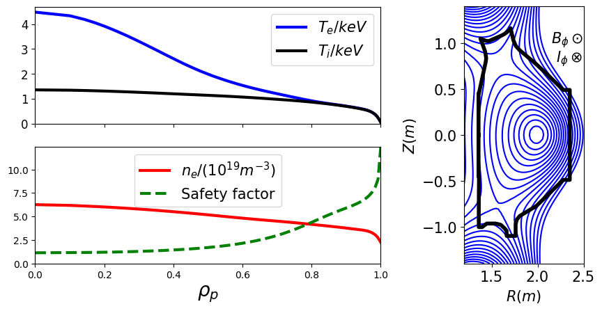
Figure 1: Left panel: profiles of electron number density $n_{e}$ , electron temperature $T_{e}$, ion temperature $T_{i}$, and safety factor $q$. Right panel: magnetic configuration. Directions of the current and toroidal magnetic field are indicated in the figure. This is a high-$\beta_{p}$ discharge with low plasma current $I_{p}=360\operatorname{kA}$, $q_{95}=7.6$, $q_{\operatorname{axis}}=1.16$, and $B_{\phi\operatorname{axis}}=-2.2T$. (All visualizations in this paper were created by using Numpyharris2020array (33), Scipy2020SciPy-NMeth (34), and MatplotlibHunter:2007 (35), which are open source Python libraries.)

In this work, we assume a Deuterium plasma with Carbon impurities, with the effective charge number of background ions being $Z_{\operatorname{eff}}=2.23$ across the entire plasma. Simulations in this work are performed by using TGCO codeyoujunhu2021 (23, 24), which models neutral beam ionization, slowing-down, collision transport, and edge loss of the resulting fast ions. We consider Deuterium NBI with full energy $E_{\operatorname{full}}=65\operatorname{keV}$, and the particle number ratio between full, half, and 1/3 energy being $80\%:14\%:6\%$ after the beam leaving from the neutralization vessel. The beam power after leaving the neutralization vessel is fixed at 1MW. We consider a reference case where NBI tangential radius is $R_{\tan}=1.26m$ and injects in the co-current direction. As a comparison, we also consider a modified scenario where the tangential radius is changed to $R_{\tan}=0.731m$.

II.2 Fast ion birth distribution

The neutral beam ionization is modeled by the Monte-Carlo methodpankin2004 (11, 23). Typical number of Monte-Carlo markers initially loaded in the simulations is $1\times 10^{5}$. The beam stopping cross section data used in the simulation are from Ref. Suzuki_1998 (36), which includes the charge exchange with thermal and impurity ions, impact ionization by electrons, thermal and impurity ions, and the multi-step ionization involving excitation states of neutrals. Beam ionization outside of the last-closed-flux-surface (LCFS) is ignored in the simulations.

Figure 2(a) and (b) plot the fast ion density in the poloidal plane (averaged over the toroidal direction) and in the toroidal plane (averaged over the vertical direction), respectively. Figure 2(c) and (d) plot the 1D histogram of the fast ions along $R$ and $\phi$, respectively. The results indicate most fast ions are born near the low-field-side. The particle and power shine-through fraction in this case is 3.8% and 4.1%, respectively. Figure 2(e) plots the deposition density profile along the minor radius, which shows that the density reach its maximum at the magnetic axis, i.e., the beam deposition is on-axis.

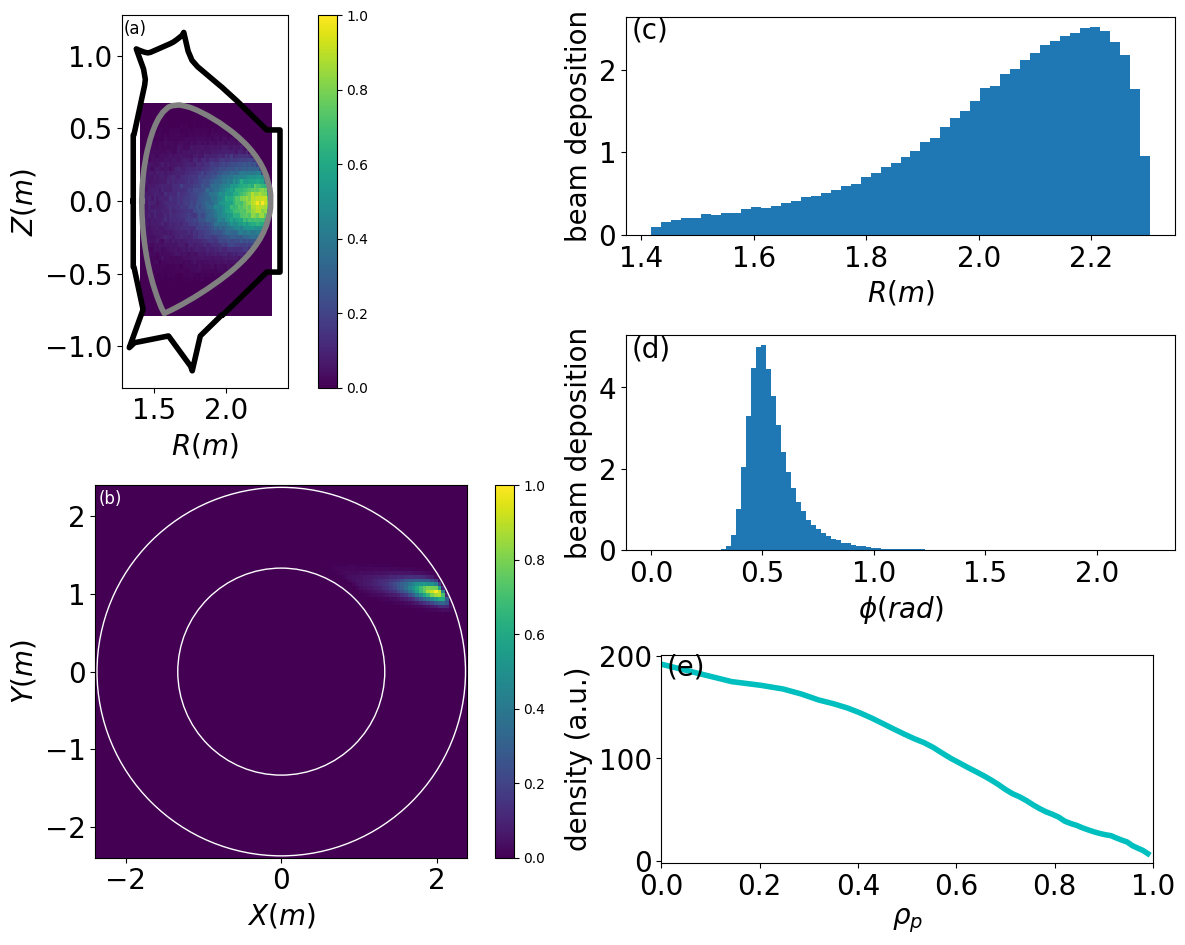
Figure 2: Neutral beam ionization density in the poloidal plane (a) and toroidal plane (b). One-dimensional histogram along $R$ and $\phi$ are also shown in (c) and (d). Panel (e) shows the density profile along the minor radius (averaged over the poloidal and toroidal direction). This is for the neutral beam injection with $R_{\tan}=1.26m$ and $E_{\operatorname{full}}=65\operatorname{keV}$ in EAST discharge #101473@4.5s. The while lines in (b) correspond to the first (inner and outer) wall. The magnetic axis is at $R=1.9m$.

It is often useful to use $(P_{\phi},\Lambda)$ coordinates to describe the phase space, where $\Lambda=\mu B_{\operatorname{axis}}/E$, $\mu$ is the magnetic moment, $E$ is the kinetic energy, and $P_{\phi}$ is the canonical toroidal angular momentum. In these coordinates, it is easier to classify orbit types. For example, whether a particles is passing or trapped can be readily identified. Figure 3 plots the fast ion birth distribution in $(P_{\phi},\Lambda)$ plane, which indicates that most of the fast ions are passing particles (the region within the dashed line triangle is the trapped region). The fraction of trapped fast ions is $0.6\%$ for this case. Figure 4 plots the birth distribution over the pitch $v_{\parallel}/v$, which shows that the dominant pitch is around $-0.6$.

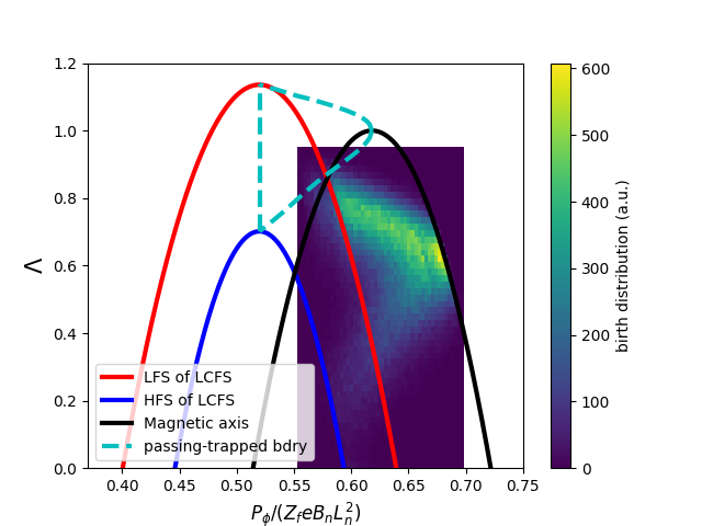
Figure 3: NBI fast ion birth distribution shown in the $(P_{\phi},\Lambda)$ plane. Also shown are the passing trapped boundary, the magnetic axis, high-field-side, and the low-field side of last-closed-flux-surface (LCFS) for fast ions of $E=65\operatorname{keV}$. Note that the pass-trapped boundary does not depend on the kinetic energy. Here $B_{n}=1T$ and $L_{n}=1m$.

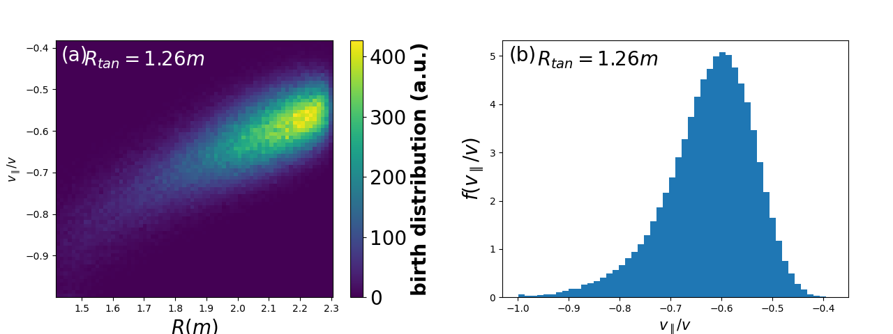
Figure 4: NBI fast ion birth distribution histogram in $(R,v_{\parallel}/v)$ (a) and in $v_{\parallel}/v$ (b).

II.3 Fast ion steady-state distribution

Fast ions born from the beam ionization are transformed to guiding-center space and the guiding-center drifts are followed by using the 4th order Runge-Kutta scheme in the cylindrical coordinates $(R,\phi,Z)$. A fast ion is considered lost/thermalized when it touches the first wall or when it slows down to the energy of $2T_{i}(0)$, where $T_{i}(0)$ is the thermal ion temperature at the magnetic axis. Charge exchange loss of fast ions Kramer_2020 (37) is not included in the simulations. The loop voltage is well controlled to be near zero during the flat-top phase, indicating fully non-inductive. Therefore, the toroidal electric field is not included in the simulation. The collision model used in this work includes the effect of slowing-down, pitch-angle scattering, and energy diffusion (the details are provided in Appendix B).

The finite Larmor radius (FLR) effect is included when (1) checking whether a fast ion touches the wall and (2) depositing guiding-center markers to spatial gridpoints to compute the distribution moment. The FLR effect is not included when pushing guiding-center trajectories since it has negligible effects.

In order to have a steady state on the slowing-down time scale, we need to include a continuous beam source. The method of including the continuous beam source is given in Appendix A.

Figure 5 plots the steady-state fast ion density distribution in the poloidal plane (left-panel) and in the toroidal plane (right-panel). The results indicate that the fast ions density is roughly poloidally uniform and toroidally uniform for the 1MW beam power. Note that the fast ion source is neither poloidally uniform nor toroidally uniform. The steady state fast ion distribution is not guaranteed to be poloidally uniform or toroidally uniform. It depends on the magnitude of beam power. For the 1MW beam power considered here, the non-uniformity in the poloidal direction and toroidal direction is negligible. The poloidal uniformity is further confirmed in Figure 6, which plots the radial profiles of various poloidal harmonics of the fast ion density. The results show that the $m=0$ harmonic is dominant ($m$ is the poloidal mode number).

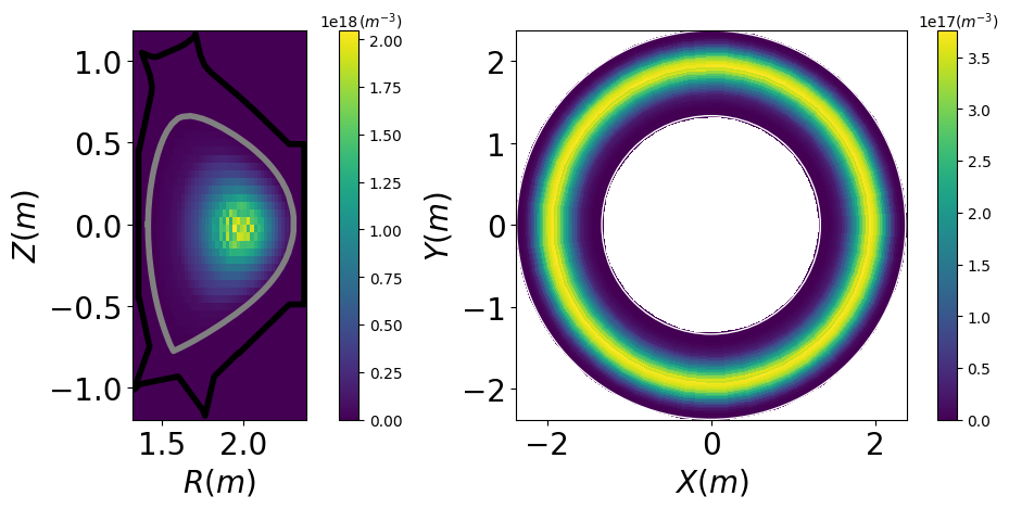
Figure 5: Fast ion density distribution in the poloidal plane (averaged over the toroidal direction) and toroidal plane (averaged over the vertical direction).

In Fig. 6, we distinguish between trapped and passing particles. The radial profile of the trapped particle fraction is also shown is Fig. 6c. The total trapped particle fraction in the steady-state distribution is $17\%$, which is significantly different from that in the birth distribution $(0.6\%)$. The pitch angle scattering can scatter particles between passing and trapped region of the phase space. Hence, it is expected the trapped fraction may be changed by collisions.

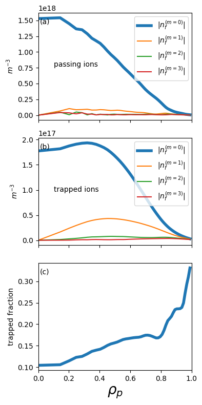
Figure 6: Radial profiles of various poloidal Fourier harmonics of passing (a) and trapped (b) fast ion densities. Shown in (c) is the radial profile of trapped fast ion fraction. The straight-field-line poloidal angle is used when doing the poloidal Fourier expansion.

Figures 7a-b plot the fast ion toroidal current density distribution in the poloidal plane. Here we distinguish the current carried by passing particles and that carried by trapped particles. The results indicate that the trapped particle current is negligible. Also note that the trapped particle currents in the core region and near the edge have opposite directions, with the edge current being in the co-current direction. This phenomenon has connection with the so-called “banana current”, which is an analogue of the diamagnetic current (the latter is due to the gyro-orbits and is in the perpendicular direction, whereas the former is due to drift-orbits and is in the parallel directionPeeters_2000 (38)). The banana current can be considered part of the bootstrap currentPeeters_2000 (38). In the case shown in Fig. 7, the current direction reverse happens at $\rho_{p}\approx 0.6$. The volume integrated trapped particle current is in the co-current direction, although being very small (only 1% of the total fast ion current). Figures 7c-d plots the poloidal harmonics of currents carried by passing ions and trapped ions. For the passing ion current, the $m=0$ harmonic is dominant, indicating poloidally uniform of the current. For the trapped ion current, the $m=1$ harmonic becomes dominant in the out region $(\rho_{p}>0.6)$, indicating poloidal nonuniform.

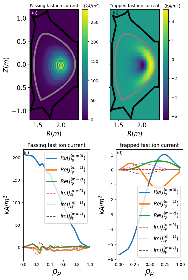
Figure 7: Distribution of passing (a) and trapped (b) fast ion toroidal current densities in the poloidal plane. Shown in (c) and (d) are the radial profiles of various poloidal Fourier harmonics of passing (c) and trapped (d) fast ion current densities.

Figures 8(a)-(e) plot the steady-state fast ion distribution in $(E,v_{\parallel}/v)$, where $E$ is the kinetic energy and $v_{\parallel}$ is the parallel (to the magnetic field) velocity. Both the 2D distribution and 1D distributions are plotted. We also distinguish between the passing particles and trapped particles. The results indicate that the trapped particle distribution is roughly symmetrical in $v_{\parallel}/v$ around $v_{\parallel}/v=0$, indicating it carries nearly zero parallel current. The results also indicate that trapped fast ions are more localized in the low energy region when compared with passing fast ions which have nearly uniform energy spectrum. There are three jumps in Fig 8(d), which correspond to the NBI source at full, half, and $1/3$ of $65\operatorname{keV}$. Note that collisional energy diffusion makes some particles exceed the full energy, as is shown in Fig 8(d).

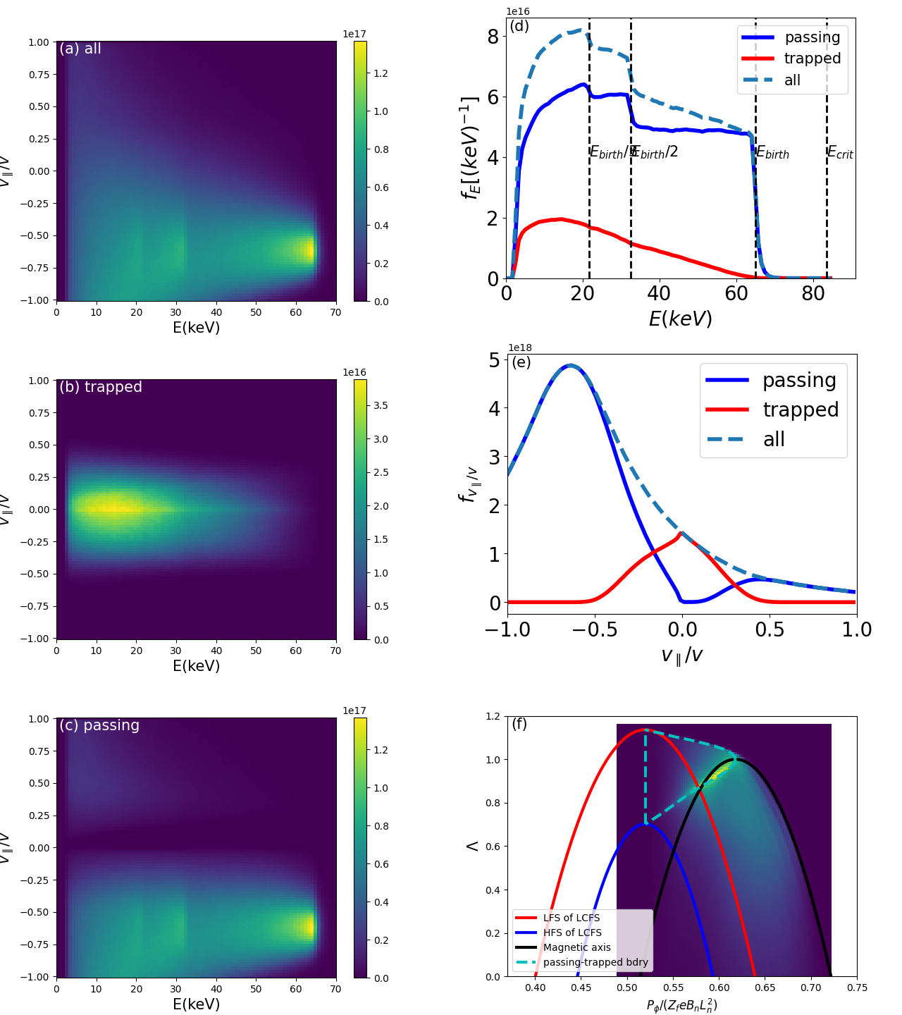
Figure 8: Steady-state distribution of NBI fast ions in $(E,v_{\parallel}/v)$ (a-c), in $E$ (d), in $v_{\parallel}/v$ (e), and in $(P_{\phi},\Lambda)$ (f). Refer to Fig. 3 for the meaning of the various lines in (f). Here $f_{E}$ is defined by $dN=f_{E}dE$, where $dN$ is the number of particles within the energy interval $dE$. And $f_{v_{\parallel}/v}$ and the 2D distributions are defined in a similar way. The critical energy for this case $E_{\operatorname{crit}}=83.6\operatorname{keV}$, which is larger than the fast ion birth energy.

Figure 8(f) plots the steady-state distribution in the $(P_{\phi},\Lambda)$ plane. The fast ions seem to reach their peak density near the passing-trapped boundary. As a comparison, the birth distribution, as is shown in Fig. 3, has no obvious structure near the passing-trapped boundary. The structure of the steady-state distribution near the passing-trapped boundary is not sensitive to the fast ion birth profile. For instance, Fig. 9 considers the  $R_{\tan}=0.731m$ beam and compares the birth distribution and steady-state one, which shows that the latter still reach its peak near the passing-trapped boundary.

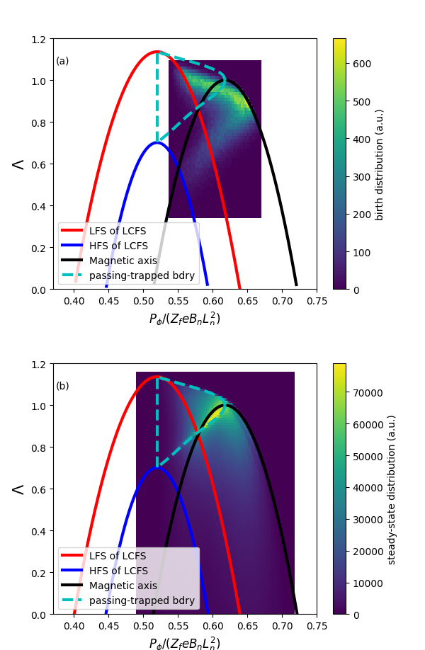
Figure 9: NBI fast ion birth distribution (a) and steady-state distribution (b) in $(P_{\phi},\Lambda)$ plane for the $R_{\tan}=0.731m$ beam.

II.4 Dependence of fast ion current on plasma current

Let us examine the dependence of NBCD on the plasma current. We change the plasma current by multiplying the poloidal magnetic flux $\Psi$ (2D data from EFIT) by a factor $\alpha_{p}$. Since the poloidal magnetic field $\mathbf{B}_{p}$ is related to $\Psi$ via

$$\mathbf{B}_{p}=-\frac{1}{R}\frac{\partial\Psi}{\partial Z}\hat{\mathbf{R}}+\frac{1}{R}\frac{\partial\Psi}{\partial R}\hat{\mathbf{Z}},$$ (1)

where $\hat{\mathbf{R}}$ and $\hat{\mathbf{Z}}$ are the cylindrical unit vectors, the above multiplication corresponds to multiplying the $\mathbf{B}_{p}$ by $\alpha_{p}$. Similarly, since the plasma toroidal current density $J_{\phi}$ is related to $\Psi$ via

$$J_{\phi}=-\mu_{0}^{-1}\frac{1}{R}\frac{\partial^{2}\Psi}{\partial Z^{2}}-\mu_{0}^{-1}\frac{\partial}{\partial R}\left(\frac{1}{R}\frac{\partial\Psi}{\partial R}\right),$$ (2)

where $\mu_{0}$ is the vacuum magnetic permeability, the above scaling also scales the plasma current $I_{p}$ by $\alpha_{p}$. We keep the values of the toroidal magnetic field $B_{\phi}$ fixed when changing $\Psi$. As a result, the safety factor $q$ is also scaled by a factor of $\alpha_{p}$. Figure 10 plots the safety factor profiles corresponding to different values of $\alpha_{p}=I_{p}/I_{p,\operatorname{ref}}$, where $I_{p,\operatorname{ref}}$ is the plasma current in the original configuration.

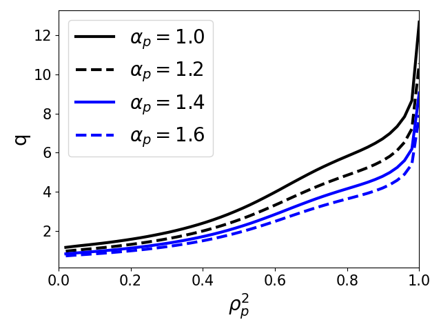
Figure 10: Safety factor radial profiles for different values of $\alpha_{p}$.

Figure 11a plots the fast ion current as a function of the plasma current, which indicates that the dependence is not monotonic: in the lower $I_{p}$ regime, the fast ion current $I_{f}$ increase with $I_{p}$ increasing whereas, in the higher $I_{p}$ regime, $I_{f}$ decreases with $I_{p}$ increasing.

The increasing of $I_{f}$ with $I_{p}$ increasing in lower $I_{p}$ regime is probably due to the improvement of fast ion confinement. The drift orbit width is inverse proportional to the poloidal magnetic fieldwesson2004 (25). Larger plasma current implies stronger poloidal magnetic field, hence smaller drift orbit width and thus better confinement of fast ions. The evidence for this is shown in Fig. 11b, which indicates that the fast ion loss fraction decreases rapidly with the plasma current increasing in the lower $I_{p}$ region.

Next, we try to understand why the fast ion current decrease with plasma current increasing in high $I_{p}$ regime. The only hint that we can identify is that the trapped fraction increase with the plasma current. The increase in trapped fraction happens for both the birth distribution and the steady-state distribution, as is shown in Fig. 11(e) and (f).

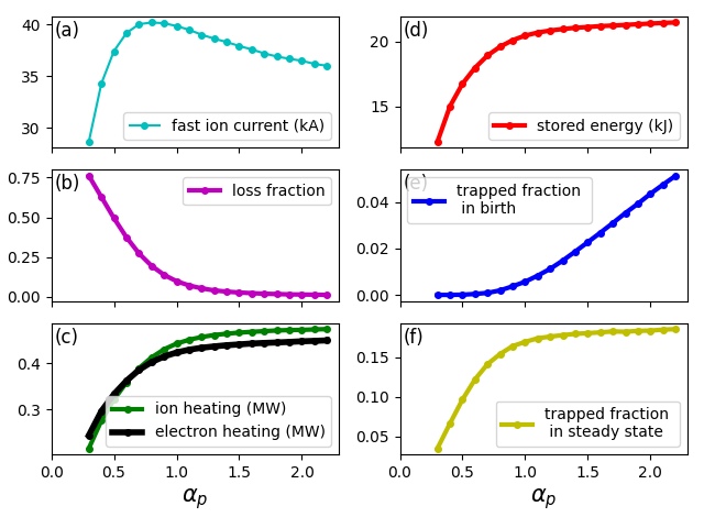
Figure 11: Fast ion toroidal current (a), edge particle loss fraction (b), ion and electron heating power (c), saturated stored energy (d), trapped fraction in birth (e), and trapped fraction in steady-state (f) as a function of the plasma current $I_{p}=\alpha_{p}I_{p,\operatorname{ref}}$.

Figure 12 plots the radial profiles of fast ion currents, the trapped fraction, and the current carried by the trapped fast ions, for various plasma currents. The results indicate again that trapped particles carry negligible current. Increasing the plasma current makes the trapped fraction increased across a wide radial region except the edge.

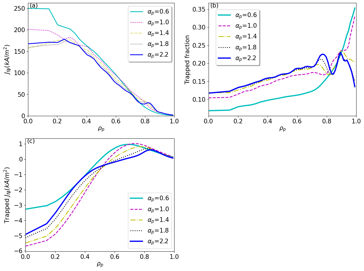
Figure 12: Radial profiles of fast ion toroidal current densities (a), trapped fractions (b), and trapped fast ion current densities (c) in magnetic configurations with different plasma currents.

We also performed similar simulations as above but with a smaller NBI tangential radius, $R_{\tan}=0.731m$. This case has larger trapped particle fraction. The results are plotted in Figs. 13 and 14. We observe the same non-monotonic dependence of the fast ion current on the plasma current. And also the results indicate that the trapped particles carry nearly zero current.

In the above scanning of plasma current, the density and temperature profiles are kept fixed. Therefore the force-balance is not guaranteed. This is a weakness of this work. Similarly, the equilibrium is not re-computed in the density scanning presented in the next section.

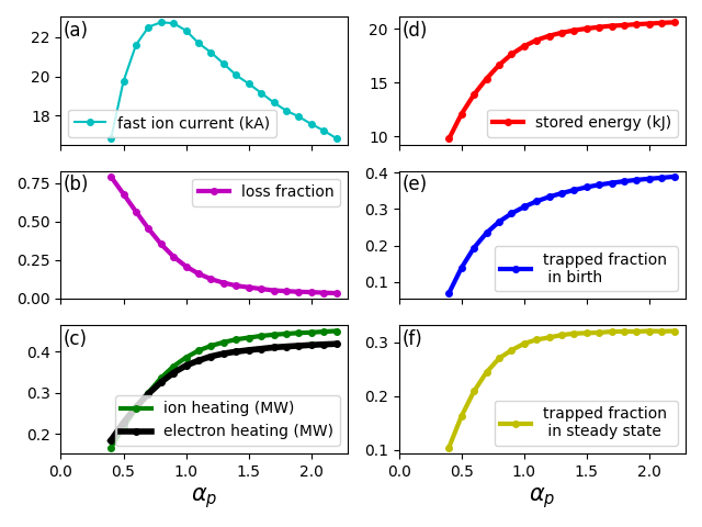
Figure 13: The same as Fig. 11 except for a smaller tangential radius, $R_{\tan}=0.731m$.

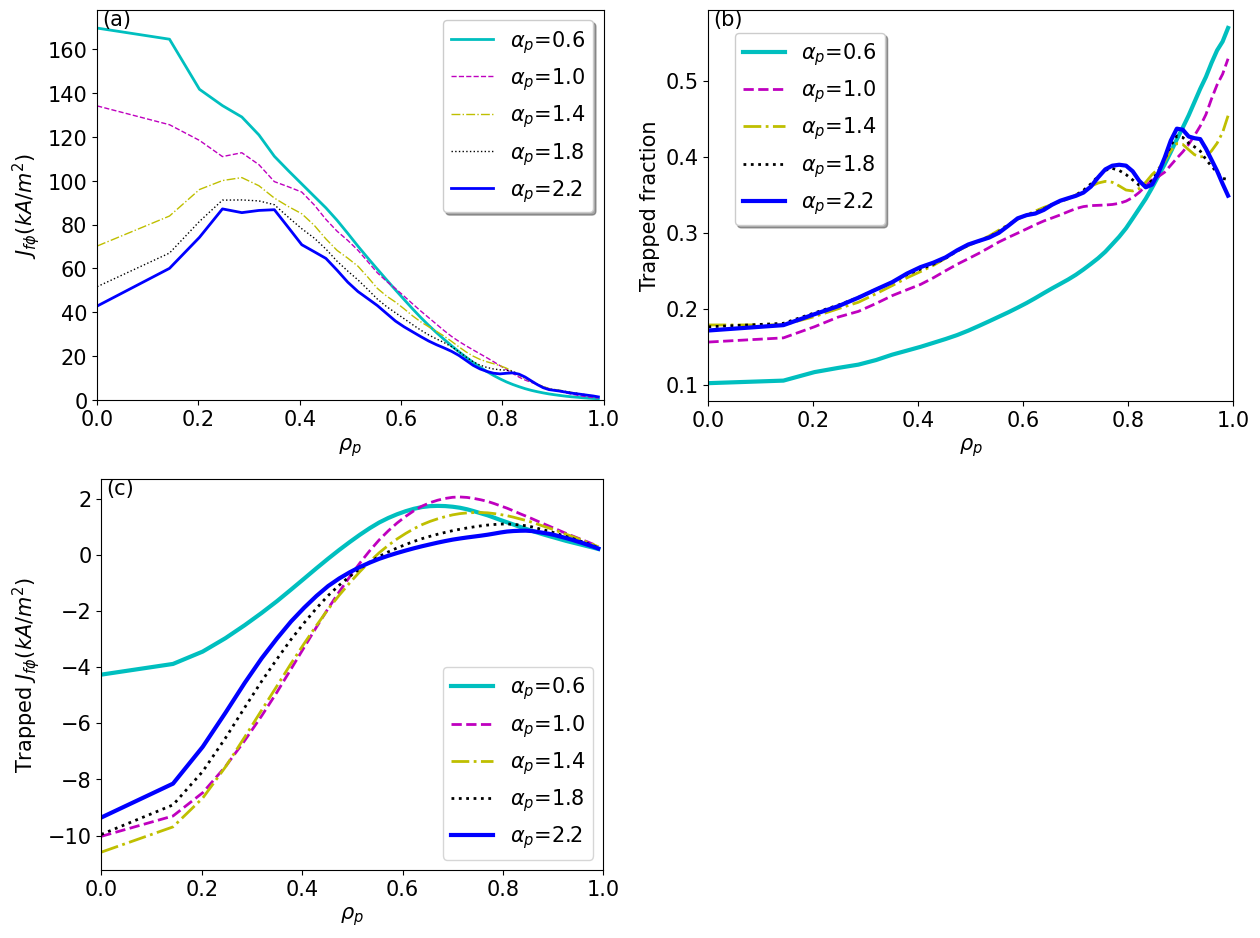
Figure 14: The same as Fig. 12 except for a smaller tangential radius, $R_{\tan}=0.731m$.

II.5 Dependence of fast ion current on plasma density

Next, we examine the plasma density dependence of fast ion current. The density affects both the ionization process and the fast ion collisional transport. The ionization process affects the shine-through fraction and ion birth location. The latter influences the first-orbit loss fraction and the ratio between trapped and passing fast ions. The collision transport influences the fast ion distribution in both position space (edge loss) and velocity space (slowing-down and passing-trapped transition). These effects may have opposite effects on the fast ion current. Therefore it is not obvious what is the trend of fast ion current changing with the plasma density. Next, we examine this trend via simulations.

We scan the electron density via scaling the profile in Fig. 1 by a factor of values ranging from $0.2$ to 1.8. Fig. 15a plots the dependence of the volume integrated fast ion current on the density, which indicates that the current decreases with increasing of the density. Fig. 15b shows that the shine-through loss decrease with the density increasing (as is expected). Also Fig. 15c shows that the ion edge loss fraction decreases with the density increasing. These reduction of loss is beneficial for current drive since more fast ions can stay in the plasma to contribute electric current. On the other hand, Fig. 15(f-h) shows that, with the density increasing, the slowing-down time becomes shorter and the trapped particle fraction becomes larger. These are deleterious effects for current drive. Shorter slowing-down time implies that fast ions can remain energetic for shorter time and thus less fast ions can contribute to the fast ion current. Larger trapped fraction means less particles can efficiently contribute to the current. The results in Fig.  15(a) indicates that the deleterious effects turn out to defeat those beneficial effects, making the fast ion current decreases with the density increasing.

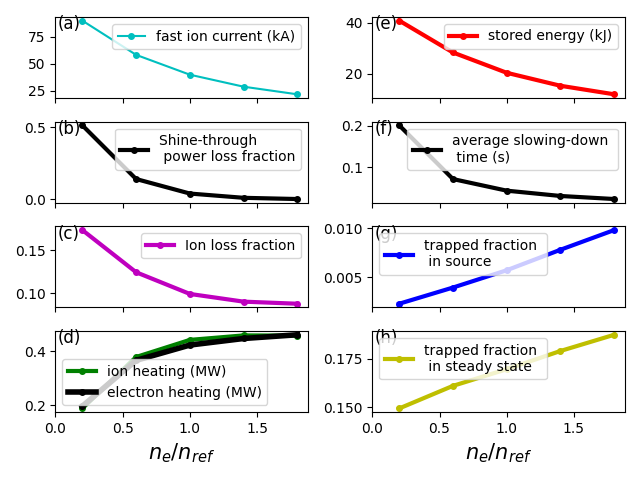
Figure 15: The plasma density dependence of fast ion current (a), shine-through loss (b), ion loss fraction (c), ion/electron heating power (d), fast ion stored energy (e), slowing-down time (f), and trapped fraction in birth distribution (g) and in steady-state distribution (h).

Figure 16 plots the radial profiles of fast ion current density. The results indicate that, for all radial positions, the fast ion current density decreases with the plasma density increasing.

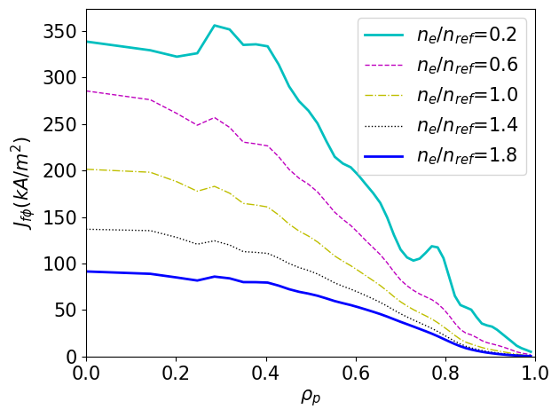
Figure 16: Radial profiles of fast ion current density for various plasma density.

II.6 Electron shielding current

Taking into account the electron shielding effect on the fast ion current does not qualitatively change the dependence of the driven current on the plasma current, i.e., net current follows a similar trend as the fast ion current, as is shown in Fig. 17 and 18.

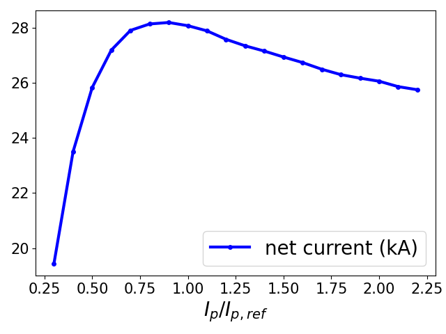
Figure 17: The same as Fig. 11a except that this is the driven current that includes the electron return current.

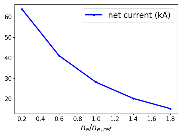
Figure 18: The same as Fig.  15a except that this is the net current rather than the fast ion current.

Figure 19 plots the radial profiles of various quantities related to the driven current, namely, the pure fast ion current density $J_{f}$, the electron shielding factor $F$, the net current density $J_{\operatorname{net}}=J_{f}F$, the effective trapped electron fraction $f_{t}$,  the electron collision frequency $\nu_{e}$, the thermal electron bounce frequency $\omega_{b}$, and the normalized electron collision frequency $\nu_{e\star}$. (The details of these quantities are given in Appendix C.) The formulas for the shielding effect used here are valid for general tokamak equilibria and arbitrary collisionality regimeHonda_2012 (28, 29), where the equilibrium shaping effects are included via the effective trapped fraction $f_{t}$.

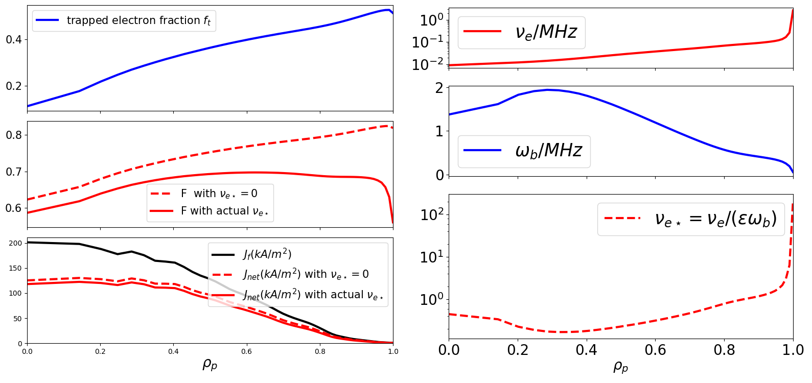
Figure 19: Radial profiles of effective trapped electron fraction $f_{t}$, the shielding factor $F$, the pure fast ion current density $J_{f}$, the net current density $J_{\operatorname{net}}=J_{f}F$, the electron collision frequency $\nu_{e}$, the thermal electron bounce frequency $\omega_{b}$, and the normalized electron collision frequency $\nu_{e\star}$. Some quantities are undefined at the magnetic axis. Their values are obtained by interpolation.

As a comparison, we also plot the shielding factor $F$ for the case of $\nu_{e\star}=0$ and the resulting net current. The results show that the $\nu_{e\star}=0$ approximation slightly overestimates the net current.

III Summary

Simulations of neutral beam current drive on the EAST tokamak were performed, providing detailed information about the fast ion distribution in both real space and velocity space. We distinguish between current carried by passing particles and that carried by trapped particles, and found that trapped ions carry co-current current near the edge and counter-current current near the core. However, the magnitude of the trapped ion current is one order smaller than that of the passing ions, making their contribution to the fast ion current negligible.

We examine the dependence of the fast ion current on the plasma current $I_{p}$. With $I_{p}$ increasing, the drift orbit width decreases, which helps reduce the first-orbit loss and collisional transport, and thus is beneficial for fast ion confinement. This mechanism makes the fast ion current increase with $I_{p}$ in the low $I_{p}$ regime. But for high $I_{p}$ regime, the effect of trapped fraction increasing becomes dominant. Since the trapped fast ions carry nearly zero current, the increasing of trapped fraction then implies the decreasing of fast ion current.

The fast ion current decreases with the increase of plasma density $n_{e}$. This dependence is mainly determined by the variation of the slowing-down time with $n_{e}$, which is already well known and is confirmed in our specific situation.

IV ACKNOWLEDGMENTS

Youjun Hu thanks  Youwen Sun, G. S. Xu, Yingfeng Xu, Lei Ye, Yifeng Zheng, and Baolong Hao for useful discussions, and thanks Xiaotao Xiao for careful reading of the first version of this paper. The manuscript of this paper was written in GNU TeXmacs, a free structured WYSIWYG editor for scientiststexmacs (39). Numerical computations were performed on Tianhe at National SuperComputer Center in Tianjin, Sugon computing center in Hefei, and the ShenMa computing cluster in Institute of Plasma Physics, Chinese Academy of Sciences. This work was supported by Users with Excellence Program of Hefei Science Center CAS under Grant No. 2021HSC-UE017, by Comprehensive Research Facility for Fusion Technology Program of China under Contract No. 2018-000052-73-01-001228, and by the National Natural Science Foundation of China under Grant No. 11575251.

IV.1 Conflict of interest

The authors have no conflicts to disclose.

V DATA AVAILABILITY

The data that support the findings of this study are available at https://github.com/Youjunhu/TGCO, and are licensed under the GNU General Public License v3.0.

Appendix A Continuous beam injection

To obtain the steady state of fast ions, we need include the continuous beam source. A straightforward Monte-Carlo implementation of this continuous injection would be to introduce new Monte-Carlo markers to represent the newly injected physical particles at each time step. This method is computationally expensive. For a time-independent background plasma, there is an efficient method that involves only a single injection and then utilizes the time shift invariant to infer the contribution of all the other injections. This method is illustrated in Fig. 20.

Figure 20: An efficient way of simulating multiple injections. The contribution of injections at $t=j\Delta t$ with $j=0,1,2$ to the fast ion distribution at $t=3\Delta t$ can be obtained by following the time history of the particles injected at $t=0$ and recording their contribution to the fast ion distribution at $t=\Delta t,2\Delta t,3\Delta t$, indicated respectively by $A1$, $A2$, and $A3$. Then it is ready to see that $B1=A1$, $B2=A2$, and $B3=A3$. Therefore the contributions of the multiply injections can be inferred from the time history of a single injection.

The above method works only for a time-independent background plasma and constant beam power. For time-dependent background plasma, re-injecting new Monte-Carlo markers seems to be the only method available. The present work considers a time-independent background plasma with a constant beam power and use the above efficient method.

Appendix B Collision model

In the zero drift-orbit width approximation, the time it takes for a fast ion of velocity $v_{1}$ to be slowed down to $v_{2}$ by the collision friction with the background ions and electrons is given bywesson2004 (25)

$$\tau_{s}=\frac{\tau_{se}}{3}\ln\left[\frac{1+\left(\frac{v_{c}}{v_{1}}\right)^{3}}{\left(\frac{v_{2}}{v_{1}}\right)^{3}+\left(\frac{v_{c}}{v_{1}}\right)^{3}}\right],$$ (3)

where $v_{c}$ is the critical velocity defined by

$$v_{c}=\left(\frac{3\sqrt{\pi}}{4}\frac{m_{e}}{n_{e}}\sum_{i}\frac{n_{i}Z_{i}^{2}}{m_{i}}\right)^{1/3}\sqrt{\frac{2T_{e}}{m_{e}}},$$ (4)

$\tau_{se}=1/\nu_{se}$ with $\nu_{se}$ defined by

$$\nu_{se}=\frac{4}{3\sqrt{\pi}}\frac{m_{f}}{m_{e}}\frac{\Gamma^{f/e}}{(2T_{e}/m_{e})^{3/2}},$$ (5)

which is the slowing-down rate due to background electrons,

$$\Gamma^{f/e}=\frac{n_{e}Z_{f}^{2}e^{4}}{4\pi\epsilon_{0}^{2}m_{f}^{2}}\ln\Lambda,$$ (6)

$\ln\Lambda$ is the Coulomb logarithm ($\ln\Lambda=24-\ln\left(10^{-6}\sqrt{n_{e}}/T_{e}\right)\approx 16.97$ is used in this work, where $n_{e}$ and $T_{e}$ are in units of $m^{-3}$ and $\operatorname{keV}$, respectively).

Both $\tau_{se}$ and $v_{c}$ have a radial dependence via their dependence on the plasma density and temperature. The radial profile of $\tau_{s}$ for the plasma specified in Fig. 1 is plotted in Fig. 21 for fast ions of $65\operatorname{keV}$ to be slowed down to a cutoff velocity (chosen as $mv_{2}^{2}/2=2T_{i}(0)$ in this article). The result shows that typical slowing-down time in the core region is about $60\operatorname{ms}$.

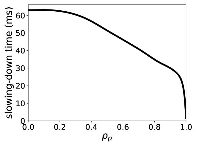
Figure 21: Radial profiles of slowing-down time for fast ions of kinetic energy $65\operatorname{keV}$ (assuming zero drift-orbit width) to slow down to the cutoff energy $2T_{i}(0)$ in the equilibrium specified in Fig. 1.

The formula (3) only includes the slowing-down, neglecting pitch-angle scattering and energy diffusion. For realistic simulations that include pitch-angle scattering, energy diffusion, finite-orbit-width effect, and non-uniform plasma profiles, we need to use numerical integration to determined the slowing-down process of fast ions. The Monte-Carlo algorithm used in this work for collision of fast ions with background electrons and ions is specified in Ref. todo2014 (40), where the pitch-angle variable $\lambda=v_{\parallel}/v$ and velocity $v$ are altered at the end of each time step according to the following scheme:

$$\lambda_{\operatorname{new}}=\lambda(1-\nu_{d}\Delta t)\pm\sqrt{(1-\lambda^{2})\nu_{d}\Delta t},$$ (7)

and

$$v_{\operatorname{new}} = v-\nu_{s}\Delta tv\left(1+\frac{v_{c}^{3}}{v^{3}}\right)$$ (8)

$$+ \frac{\nu_{s}\Delta t}{m_{f}v}\left[T_{e}-\frac{1}{2}T_{i}\left(\frac{v_{c}}{v}\right)^{3}\right]$$

$$\pm \sqrt{\frac{\nu_{s}\Delta t}{m_{f}}\left[T_{e}+T_{i}\left(\frac{v_{c}}{v}\right)^{3}\right]}$$

where the second and third line correspond to the energy diffusion, $\pm$ denotes a randomly chosen sign with equal probability for plus and minus, $\Delta t$ is the time step, $\nu_{d}$ is the pitch-angle scattering rate given by

$$\nu_{d}=\left(\frac{Z_{\operatorname{eff}}}{v^{3}}\right)\frac{n_{e}Z_{f}^{2}e^{4}\ln\Lambda}{4\pi\varepsilon_{0}^{2}m_{f}^{2}},$$ (9)

where $Z_{f}$ is the charge number of fast ions, $\nu_{s}$ is the slowing down rate given by Eq. (5).

Appendix C Formulas for electron shielding effect

The electron collision time (characterizing electron collision with ions) iswesson2004 (25)

$$\tau_{e}=\frac{12\pi^{3/2}}{\sqrt{2}}\dfrac{\varepsilon_{0}^{2}\sqrt{m_{e}}T_{e}^{3/2}}{n_{i}Z_{i}^{2}e^{4}\ln\Lambda_{e}},$$ (10)

where $\varepsilon_{0}$ is the vacuum permittivity, $\ln\Lambda_{e}$ is the Coulomb logarithm for electron-ion collision ($\ln\Lambda_{e}=15.2-0.5\ln(n_{e}/10^{20})+\ln(T_{e})$ is used in this work, where $n_{e}$ and $T_{i}$ are in units of $m^{-3}$ and $\operatorname{keV}$, respectively). The dimensionless electron collision parameter $\nu_{e\star}$ is defined by

$$\nu_{e\star}=\frac{\nu_{e}}{\varepsilon\omega_{be}},$$ (11)

where $\nu_{e}=1/\tau_{e}$, $\varepsilon=r/R_{0}$ is the local inverse aspect ratio, $r=(R_{\max}-R_{\min})/2$, $R_{0}=(R_{\min}+R_{\max})/2$, $R_{\min}$ and $R_{\max}$ are, respectively, the maximal and minimal values of the cylindrical coordinate $R$ on a magnetic surface, $\omega_{be}$ is the typical bounce (angular) frequency of thermal electrons, which is given by (in the approximation of zero-orbit-width and deeply trapped electrons)

$$\omega_{be}=\frac{\sqrt{2T_{e}/m_{e}}}{qR_{0}}\left(\frac{\varepsilon}{2}\right)^{1/2},$$ (12)

where $q$ is the safety factor of the magnetic surface. Using this, Eq. (11) is written as

$$\nu_{e\star}\equiv\frac{\nu_{e}}{\varepsilon^{3/2}\sqrt{T_{e}/m_{e}}/(qR_{0})}.$$ (13)

Due to the electron shielding effect, the ratio of the net current to the fast ion current is given by

$$F\equiv\frac{\langle j_{\parallel}B\rangle}{\langle j_{f\parallel}B\rangle}=1-\frac{Z_{f}}{Z_{\operatorname{eff}}}(1-\mathcal{L}_{31}),$$ (14)

where $\langle\ldots\rangle$ is the magnetic surface averaging,  $\mathcal{L}_{31}$ is the bootstrap current coefficient before the electron density gradient. The formula of $\mathcal{L}_{31}$ given by Sauter et al.sauter1999 (27) is

$$\mathcal{L}_{31} = \left(1+\frac{1.4}{Z_{\operatorname{eff}}+1}\right)X-\frac{1.9}{Z_{\operatorname{eff}}+1}X^{2}$$ (15)

$$+ \frac{0.3}{Z_{\operatorname{eff}}+1}X^{3}+\frac{0.2}{Z_{\operatorname{eff}}+1}X^{4},$$

with

$$X=\frac{f_{t}}{1+(1-0.1f_{t})\sqrt{\nu_{e\star}}+0.5(1-f_{t})\nu_{e\star}/Z_{\operatorname{eff}}},$$ (16)

$f_{t}$ is the effective trapped fractionHirshman_1981 (41, 42),

$$f_{t}=1-\frac{3}{4}\left\langle\frac{B^{2}}{B_{\max}^{2}}\right\rangle\int_{0}^{1}\frac{\lambda d\lambda}{\left\langle\sqrt{1-\lambda B/B_{\max}}\right\rangle},$$ (17)

where $B_{\max}$ is the maximal value of magnetic field strength on a magnetic surface.

References

- (1) J. Scoville, M. Boyer, B. Crowley, N. Eidietis, C. Pawley, and J. Rauch, Fusion Engineering and Design 146, 6 (2019), SI:SOFT-30.
- (2) C. Hu, Y. Xie, Y. Xie, S. Liu, Y. Xu, L. Liang, C. Jiang, P. Sheng, Y. Gu, J. Li, and Z. Liu, Plasma Science and Technology 17, 817 (2015).
- (3) M. Schneider, L.-G. Eriksson, I. Jenkins, J. Artaud, V. Basiuk, F. Imbeaux, T. Oikawa, and and, Nuclear Fusion 51, 063019 (2011).
- (4) O. Asunta, J. Govenius, R. Budny, M. Gorelenkova, G. Tardini, T. Kurki-Suonio, A. Salmi, and S. Sipilä, Computer Physics Communications 188, 33 (2015).
- (5) W. W. Heidbrink, M. Murakami, J. M. Park, C. C. Petty, M. A. V. Zeeland, J. H. Yu, and G. R. McKee, Plasma Physics and Controlled Fusion 51, 125001 (2009).
- (6) R. J. Buttery, B. Covele, J. Ferron, A. Garofalo, C. T. Holcomb, T. Leonard, J. M. Park, T. Petrie, C. Petty, G. Staebler, E. J. Strait, and M. Van Zeeland, Journal of Fusion Energy 38, 72 (2019).
- (7) J. M. Park, M. Murakami, C. C. Petty, W. W. Heidbrink, T. H. Osborne, C. T. Holcomb, M. A. V. Zeeland, R. Prater, T. C. Luce, M. R. Wade, M. E. Austin, N. H. Brooks, R. V. Budny, C. D. Challis, J. C. DeBoo, J. S. deGrassie, J. R. Ferron, P. Gohil, J. Hobirk, E. M. Hollmann, R. M. Hong, A. W. Hyatt, J. Lohr, M. J. Lanctot, M. A. Makowski, D. C. McCune, P. A. Politzer, H. E. S. John, T. Suzuki, W. P. West, E. A. Unterberg, and J. H. Yu, Phys. Plasmas 16, 092508 (2009).
- (8) T. Oikawa, J. Park, A. Polevoi, M. Schneider, G. Giruzzi, M. Murakami, K. Tani, A. Sips, C. Kesse, W. Houlberg, S. Konovalov, K. Hamamatsu, V. Basiuk, A. Pankin, D. McCune, R. Budny, Y.-S. Na, I.Voitsekhovich, and S. Suzuki, 22nd IAEA Fusion Energy Conference IT/P6-5 (2008).
- (9) M. Kraus, TRANSP Current Drive Algorithms (http://w3.pppl.gov/transp/papers/).
- (10) S. Mulas, Ã. Cappa, J. Martà nez-Fernández, D. L. Bruna, J. Velasco, T. Estrada, J. Gómez-Manchón, M. Liniers, K. McCarthy, I. Pastor, F. Medina, E. Ascasíbar, and T. Team, Nuclear Fusion 63, 066026 (2023).
- (11) A. Pankin, D. McCune, R. Andre, G. Bateman, and A. Kritz, Computer Physics Communications 159, 157 (2004).
- (12) K. Tani, M. Azumi, H. Kishimoto, and S. Tamura, Journal of the Physical Society of Japan 50, 1726 (1981).
- (13) E. Hirvijoki, O. Asunta, T. Koskela, T. Kurki-Suonio, J. Miettunen, S. Sipilä, A. Snicker, and S. Äkäslompolo, Computer Physics Communications 185, 1310 (2014).
- (14) R. B. White, N. Gorelenkov, W. W. Heidbrink, and M. A. V. Zeeland, Plasma Physics and Controlled Fusion 52, 045012 (2010).
- (15) G. J. Kramer, R. V. Budny, A. Bortolon, E. D. Fredrickson, G. Y. Fu, W. W. Heidbrink, R. Nazikian, E. Valeo, and M. A. V. Zeeland, Plasma Physics and Controlled Fusion 55, 025013 (2013).
- (16) D. Pfefferlé, W. Cooper, J. Graves, and C. Misev, Computer Physics Communications 185, 3127 (2014).
- (17) Y. Xu, W. Guo, Y. Hu, L. Ye, X. Xiao, and S. Wang, Computer Physics Communications 244, 40 (2019).
- (18) K. He, Y. Sun, B. Wan, S. Gu, M. Jia, and Y. Hu, Nuclear Fusion 61, 016009 (2020).
- (19) F. Wang, R. Zhao, Z.-X. Wang, Y. Zhang, Z.-H. Lin, S.-J. Liu, and C. Team, Chinese Physics Letters 38, 055201 (2021).
- (20) M. Taguchi, Nuclear Fusion 36, 657 (1996).
- (21) S. P. Hirshman, Phys. Fluids 23, 1238 (1980).
- (22) B. Wan, Y. Liang, X. Gong, N. Xiang, G. Xu, Y. Sun, L. Wang, J. Qian, H. Liu, L. Zeng, L. Zhang, X. Zhang, B. Ding, Q. Zang, B. Lyu, A. Garofalo, A. Ekedahl, M. Li, F. Ding, S. Ding, H. Du, D. Kong, Y. Yu, Y. Yang, Z. Luo, J. Huang, T. Zhang, Y. Zhang, G. Li, T. Xia, and and, Nuclear Fusion 59, 112003 (2019).
- (23) Y. Hu, Y. Xu, B. Hao, G. Li, K. He, Y. Sun, L. Li, J. Wang, J. Huang, L. Ye, X. Xiao, F. Wang, C. Pan, and Y. Xu, Physics of Plasmas 28, 122502 (2021).
- (24) Y. Xu, L. Li, Y. Hu, Y. Liu, W. Guo, L. Ye, and X. Xiao, Nuclear Fusion 60, 086013 (2020).
- (25) J. Wesson, Tokamaks, Oxford University Press, 2004.
- (26) Y. R. Lin-Liu and F. L. Hinton, Physics of Plasmas 4, 4179 (1997).
- (27) O. Sauter, C. Angioni, and Y. R. Lin-Liu, Phys. Plasmas 6, 2834 (1999).
- (28) M. Honda, M. Kikuchi, and M. Azumi, Nuclear Fusion 52, 023021 (2012).
- (29) Y. J. Hu, Y. M. Hu, and Y. R. Lin-Liu, Phys. Plasmas 19, 034505 (2012).
- (30) B. Wan, Y. Liang, X. Gong, J. Li, N. Xiang, G. Xu, Y. Sun, L. Wang, J. Qian, H. Liu, X. Zhang, L. Hu, J. Hu, F. Liu, C. Hu, Y. Zhao, L. Zeng, M. Wang, H. Xu, G. Luo, A. Garofalo, A. Ekedahl, L. Zhang, X. Zhang, J. Huang, B. Ding, Q. Zang, M. Li, F. Ding, S. Ding, B. Lyu, Y. Yu, T. Zhang, Y. Zhang, G. Li, T. Xia, and and, Nuclear Fusion 57, 102019 (2017).
- (31) L. Lao, H. S. John, R. Stambaugh, A. Kellman, and W. Pfeiffer, Nucl. Fusion 25, 1611 (1985).
- (32) Y. C. Hu, L. Ye, X. Z. Gong, A. M. Garofalo, J. P. Qian, J. Huang, B. Zhang, P. F. Zhao, Y. J. Hu, Q. L. Ren, J. Y. Zhang, X. X. Zhang, R. R. Liang, and Z. H. Wang, Plasma Physics and Controlled Fusion 65, 055023 (2023).
- (33) C. R. Harris, K. J. Millman, S. J. van der Walt, R. Gommers, P. Virtanen, D. Cournapeau, E. Wieser, J. Taylor, S. Berg, N. J. Smith, R. Kern, M. Picus, S. Hoyer, M. H. van Kerkwijk, M. Brett, A. Haldane, J. F. del Río, M. Wiebe, P. Peterson, P. Gérard-Marchant, K. Sheppard, T. Reddy, W. Weckesser, H. Abbasi, C. Gohlke, and T. E. Oliphant, Nature 585, 357 (2020).
- (34) P. Virtanen, R. Gommers, T. E. Oliphant, M. Haberland, T. Reddy, D. Cournapeau, E. Burovski, P. Peterson, W. Weckesser, J. Bright, S. J. van der Walt, M. Brett, J. Wilson, K. J. Millman, N. Mayorov, A. R. J. Nelson, E. Jones, R. Kern, E. Larson, C. J. Carey, İ. Polat, Y. Feng, E. W. Moore, J. VanderPlas, D. Laxalde, J. Perktold, R. Cimrman, I. Henriksen, E. A. Quintero, C. R. Harris, A. M. Archibald, A. H. Ribeiro, F. Pedregosa, P. van Mulbregt, and SciPy 1.0 Contributors, Nature Methods 17, 261 (2020).
- (35) J. D. Hunter, Computing in Science & Engineering 9, 90 (2007).
- (36) S. Suzuki, T. Shirai, M. Nemoto, K. Tobita, H. Kubo, T. Sugie, A. Sakasai, and Y. Kusama, Plasma Physics and Controlled Fusion 40, 2097 (1998).
- (37) G. Kramer, M. van Zeeland, and A. Bortolon, Nuclear Fusion 60, 086016 (2020).
- (38) A. G. Peeters, Plasma Physics and Controlled Fusion 42, B231 (2000).
- (39) J. van der Hoeven, Gnu texmacs, a structured wysiwyw (what you see is what you want) editor for scientists, http://www.texmacs.org/, 2007, [Online].
- (40) Y. Todo, M. V. Zeeland, A. Bierwage, and W. Heidbrink, Nucl. Fusion 54, 104012 (2014).
- (41) S. Hirshman and D. Sigmar, Nuclear Fusion 21, 1079 (1981).
- (42) Y. R. Lin-Liu and R. L. Miller, Phys. Plasmas 2, 1666 (1995).