Consistent least squares estimation in population-size-dependent branching processes

Abstract

We consider discrete-time parametric population-size-dependent branching processes (PSDBPs) with almost sure extinction and propose a new class of weighted least-squares estimators based on a single trajectory of population size counts. We prove that, conditional on non-extinction up to a finite time $n$, our estimators are consistent and asymptotic normal as $n\to\infty$. We pay particular attention to estimating the carrying capacity of a population. Our estimators are the first conditionally consistent estimators for PSDBPs, and more generally, for Markov models for populations with a carrying capacity. Through simulated examples, we demonstrate that our estimators outperform other least squares estimators for PSDBPs in a variety of settings. Finally, we apply our methods to estimate the carrying capacity of the endangered Chatham Island black robin population.

Keywords: branching process; population-size-dependence; almost sure extinction; inference; carrying capacity; least-squares estimation; consistency.

MSC 2020: 60J80.

1 Introduction and main results

Biological populations generally display logistic growth: after an initial period of exponential growth, competition for limited resources such as food, habitat, and breeding opportunities causes population growth to slow down until the population eventually reaches a carrying capacity, which is the maximum population size that a habitat can support. Biologists often aim to estimate the carrying capacity of the habitat of the population they are studying. One example is the Chatham Island black robin population (New Zealand), which was saved from the brink of extinction in the early 1980s when it was considered the world’s most endangered bird species [4]. The population has since recovered from a single breeding female to over 120 females, and appears to be nearing carrying capacity of its habitat (Rangatira Island) [18, 17]. In order to estimate the carrying capacity, ecologists often rely on assessing environmental characteristics of the habitat itself. For example, in [17] the carrying capacity of the black robin population is estimated to be 170 nesting pairs based on a habitat suitability model which requires precise knowledge of the habitat and is very costly. Here we take a different statistical approach to estimate the carrying capacity based solely on annual population size counts using stochastic population models.

In this paper we model biological populations with discrete-time population-size-dependent branching processes (PSDBPs), which can capture fundamental properties of many populations (including logistic growth). PSDBPs are Markov chains $\{Z_{n}\}_{n\geq 0}$ characterised by the recursion

$$Z_{n+1}=\sum^{Z_{n}}_{i=1}\xi_{n,i}(Z_{n}),\qquad n\in\mathbb{N}_{0}:=\{0,1,2,\dots\},$$ (1)

where $Z_{n}$ represents the population size at time $n$ and $\{\xi_{n,i}(\cdot)\}_{n,i}$ are independent random variables that represent each individual’s offspring whose distribution depends only on the current population size $Z_{n}$. In these processes, state 0 is absorbing, and represents extinction of the population. Let $m(z):=\mathbb{E}[\xi(z)]$ denote the mean offspring at population size $z$; we say that a PSDBP has a carrying capacity $K$ if

$$m(z)>1\quad\text{when $z<K$}\quad\text{and}\quad m(z)<1\quad\text{when $z>K$}.$$ (2)

When such a threshold value $K$ exists, the PSDBP becomes extinct with probability one; this is common to almost all stochastic population models with a carrying capacity [11]. We point out that, while closely related, the mathematical definition of the carrying capacity in (2) is not the same as the biological definition given above.

The fact that PSDBPs with a carrying capacity become extinct with probability one introduces several technical challenges. For example, to perform an asymptotic analysis of an estimator $\widehat{\boldsymbol{\theta}}_{n}$ based on a single trajectory, one needs to condition on non-extinction up to a finite time $n$ —an event with vanishing probability as $n\to\infty$. Consequently, an estimator $\widehat{\boldsymbol{\theta}}_{n}$ may not satisfy the classical consistency property called $C$-consistency, defined as follows: an estimator $\widehat{\boldsymbol{\theta}}_{n}:=\widehat{\boldsymbol{\theta}}_{n}(Z_{0},\ldots,Z_{n})$ is called $C$-consistent for a parameter $\boldsymbol{\theta}$ if,

$$\textrm{for any $\varepsilon>0$,}\qquad\lim_{n\to\infty}\mathbb{P}(|\widehat{\boldsymbol{\theta}}_{n}-\boldsymbol{\theta}|>\varepsilon\,|\,Z_{n}>0)=0$$ (3)

(see for instance [19]). In [2, Theorem 1] the authors show that the maximum likelihood estimators (MLEs) $\hat{m}_{n}(z)$ (defined in (14)) for $m(z)$ in a PSDBP are not $C$-consistent but instead are such that,

$$\textrm{for any $\varepsilon>0$,}\qquad\lim_{n\to\infty}\mathbb{P}(|\hat{m}_{n}(z)-m^{\uparrow}(z)|>\varepsilon\,|\,Z_{n}>0)=0,$$ (4)

where $m^{\uparrow}(z)$ is different from $m(z)$, and can be interpreted as the mean number of offspring born to individuals when the current population size is $z$ in the $Q$-process associated with $\{Z_{n}\}$, which corresponds to $\{Z_{n}\}$ conditioned on non-extinction in the distant future (see Section 2.2). In [2] the authors refer to (4) as $Q$-consistency. A major gap remains to be filled in the context of PSDBPs with a carrying capacity: there does not exist any $C$-consistent estimator for $m(z)$ or for parameters (such as the carrying capacity) in parametric models. We point out that $C$-consistent estimators are lacking not only for PSDBPs but for any stochastic population process with a carrying capacity and an absorbing state at 0 (for example, the diffusion models in [16], the continuous-time birth-death processes in [9], and the controlled branching processes in [6]).

In this paper, we derive the first $C$-consistent estimators $\widehat{\boldsymbol{\theta}}_{n}$ for any set of parameters $\boldsymbol{\theta}$ of parametric PSDBPs (under some regularity conditions); in particular, this leads to the first $C$-consistent estimators for the carrying capacity $K$. The key idea behind our $C$-consistent estimators is to embed the $Q$-consistent MLEs $\hat{m}_{n}(z)$ and their conditional limit ${m}^{\uparrow}(z)$ in the objective function of a weighted least squares estimator,

$$\widehat{\boldsymbol{\theta}}_{n}:=\arg\min_{\theta\in\Theta}\sum_{z\geq 1}\hat{w}_{n}(z)\left\{\hat{m}_{n}(z)-{m}^{\uparrow}(z,\boldsymbol{\theta})\right\}^{2},$$ (5)

with weights $\hat{w}_{n}(z):=\hat{w}_{n}(z;Z_{0},\dots,Z_{n})$. As detailed in Section 3, this estimator differs from classical least squares estimators for stochastic processes (see for instance [13]) where the sum is taken over the successive times $i=1,\dots,n$ rather than the population sizes $z\geq 1$. To establish $C$-consistency and asymptotic normality of $\widehat{\boldsymbol{\theta}}_{n}$, we build on the asymptotic properties of $\hat{m}_{n}(z)$ and overcome several new technical challenges which arise due to the almost sure extinction of the process, as well as the implicit form of the estimator $\widehat{\boldsymbol{\theta}}_{n}$ and the fact that it includes an infinite sum.

Many populations, such as the Chatham Island black robins, are studied because they are still alive and conservation measures may need to be taken to preserve them. In these situations, the data should be viewed as being generated under the condition $Z_{n}>0$. This suggests that for many populations (particularly small populations), $C$-consistent estimators may be desirable. We demonstrate the quality of our $C$-consistent estimators on simulated data in two contexts: (i) on growing populations that are yet to reach carrying capacity, and (ii) on (quasi-)stable populations that are fluctuating around the carrying capacity. In particular, we compare our $C$-consistent estimators $\widehat{\boldsymbol{\theta}}_{n}$ with their counterpart obtained by replacing ${m}^{\uparrow}(z,\boldsymbol{\theta})$ with ${m}(z,\boldsymbol{\theta})$ in (5) (which is not $C$-consistent). We find that when the data include small population sizes (such as for the black robins), our $C$-consistent estimators $\widehat{\boldsymbol{\theta}}_{n}$ outperforms its counterpart. Finally, we apply our methods to estimate the carrying capacity of the black robin population on Rangatira Island under several PSDBP models.

The paper is organised as follows. In the next section, we provide some background on PSDBPs and their associated $Q$-process, and we introduce a flexible class of parametric PSDBPs which will serve as an illustrative example. In Section 3 we introduce our weighted least squares estimators $\widehat{\boldsymbol{\theta}}_{n}$ and in Section 4 we state their asymptotic properties. In Section 5, we compare our least squares estimators $\widehat{\boldsymbol{\theta}}_{n}$ with their counterpart obtained by replacing ${m}^{\uparrow}(z,\boldsymbol{\theta})$ with ${m}(z,\boldsymbol{\theta})$ in (5) on simulated numerical examples. In Section 6 we apply our least squares estimators to the black robin data and estimate the carrying capacity of the population. Finally, Section 7 contains the proofs of our results.

2 Background

2.1 Parametric families of PSDBPs

A discrete-time population-size-dependent branching process (PSDBP) is a Markov chain $\{Z_{n}\}_{n\in\mathbb{N}_{0}}$ characterised by the recursion given in (1) with $Z_{0}=N$, where $N$ is a positive integer, and where $\{\xi_{ni}(z):i=1,\ldots,z;\ z,n\in\mathbb{N}_{0}\}$ is a family of independent random variables with distribution $\boldsymbol{p}(z)=(p_{k}(z))_{k\in\mathbb{N}_{0}}$ such that $p_{k}(z)=\mathbb{P}[\xi_{01}(z)=k]$ depends on $z$. We refer to $\boldsymbol{p}(z)$ as the offspring distribution at population size $z$. In $\{Z_{n}\}$ the state $0$ is absorbing, and under minor regularity assumptions, all other states are transient [10].

In this paper we assume that the family of offspring distributions $(\boldsymbol{p}(z))_{z\in\mathbb{N}}$ belongs to some parametric family, that is, we assume that there exists

$$\boldsymbol{\theta}_{0}\in int(\Theta)\subseteq\mathbb{R}^{d}\qquad\text{such that}\qquad\boldsymbol{p}(z)\equiv\boldsymbol{p}(z,\boldsymbol{\theta}_{0}),\quad\text{for each}\quad z\in\mathbb{N},$$

where $int(\Theta)$ denotes the interior of the parameter space $\Theta$, and $d<\infty$. As a consequence the PSDBP is parameterised by $\boldsymbol{\theta}_{0}$. We assume that the map $\boldsymbol{\theta}\mapsto\boldsymbol{p}(z,\boldsymbol{\theta})$ is a measurable function such that $p_{k}(z,\cdot)$ is continuous on $\Theta$ for each $k\in\mathbb{N}_{0}$ and $z\in\mathbb{N}$, and is such that the offspring mean $m(z)\equiv m(z,\boldsymbol{\theta})$ and variance $\sigma^{2}(z)\equiv\sigma^{2}(z,\boldsymbol{\theta})$ are continuous on $\Theta$ for each $z\in\mathbb{N}$. In this framework, our aim is to estimate the parameter $\boldsymbol{\theta}_{0}$ based on the sample of the population sizes $\mathcal{Z}_{n}:=\{Z_{0},\ldots,Z_{n}\}$.

2.2 The $Q$-process associated with $\{Z_{n}\}$

Let $Q=(Q_{ij})_{i,j\in\mathbb{N}}$ refer to the sub-stochastic transition probability matrix of $\{Z_{n}\}_{n\in\mathbb{N}_{0}}$ restricted to the transient states $\{1,2,\ldots\}$. The entry $Q_{ij}$ is the probability that the population transitions from size $i$ to size $j$ in a single time unit. The $i$th row of $Q$ thus corresponds to the $i$-fold convolution of the offspring distribution at population size $i$. Because the family of offspring distributions $(\boldsymbol{p}(z))_{z\in\mathbb{N}}$ depends on $\boldsymbol{\theta}_{0}$, so does the transition probability matrix, and consequently, $Q\equiv Q(\boldsymbol{\theta}_{0})$, where this shorthand notation extends naturally to any $\boldsymbol{\theta}\in\Theta$.

We assume the following regularity conditions hold throughout the paper:

Assumption 1.

For each $\boldsymbol{\theta}\in\Theta$,

1. The matrix $Q(\boldsymbol{\theta})$ is irreducible.

2. $\limsup_{z\to\infty}m(z,\boldsymbol{\theta})<1$.

3. For each $\nu\in\mathbb{N}$, $\sup_{z\in\mathbb{N}}\sum_{k=1}^{\infty}k^{\nu}p_{k}(z,\boldsymbol{\theta})<\infty$.

Under Assumptions (C1)–(C3), the PSDBP becomes extinct almost surely for any $\boldsymbol{\theta}\in\Theta$ and initial state $Z_{0}=i$ (see [7, Proposition 3.1]), that is, $\mathbb{P}_{i}(Z_{n}\to 0)=1$, where $\mathbb{P}_{i}(\cdot)$ denotes the probability measure given the initial state is $i$. In addition, there exists $\rho$, $\boldsymbol{u}$, and $\boldsymbol{v}$ where $\rho:=\rho(Q)=\lim_{n\rightarrow\infty}(Q^{n})_{ij}^{1/n}$, and $\boldsymbol{u}$ and $\boldsymbol{v}$ are strictly positive column vectors such that

$$\boldsymbol{u}^{\top}Q=\rho\boldsymbol{u}^{\top},\quad Q\boldsymbol{v}=\rho\boldsymbol{v},\quad\boldsymbol{u}^{\top}\boldsymbol{1}=1,\quad\textrm{and}\quad\boldsymbol{u}^{\top}\boldsymbol{v}=1,$$ (6)

and

$$Q^{n}\sim\rho^{n}\boldsymbol{v}\boldsymbol{u}^{\top},\quad\textrm{as $n\rightarrow\infty$};$$ (7)

see for instance [7]. The vector $\boldsymbol{u}$ corresponds to the quasi-stationary (or quasi-limiting) distribution of $\{Z_{n}\}$, and the vector $\boldsymbol{v}$ records the relative “strength” of each state. We refer the reader to [2, Section 2.3] for a more detailed explanation.

For every $n\in\mathbb{N}_{0}$ fixed, the process $\{Z_{\ell}\}_{0\leq\ell\leq n}$ conditioned on $Z_{n}>0$ is a time-inhomogeneous Markov chain that we denote by $\{Z_{\ell}^{(n)}\}_{0\leq\ell\leq n}$ and whose one-step transition probabilities are

$$\mathbb{P}(Z_{\ell+1}^{(n)}=j\,|\,Z_{\ell}^{(n)}=i):=\mathbb{P}(Z_{\ell+1}=j\,|\,Z_{\ell}=i,\;Z_{n}>0)=Q_{ij}\,\dfrac{\boldsymbol{e}_{j}^{\top}Q^{n-\ell-1}\boldsymbol{1}}{\boldsymbol{e}_{i}^{\top}Q^{n-\ell}\boldsymbol{1}}\quad\text{ for }i,j\geq 1,$$ (8)

where $\boldsymbol{e}_{i}$ is a column vector whose $i$th entry is equal to 1 and whose remaining entries are 0. Taking the limit as $n\rightarrow\infty$ in (8) and using (7) leads to homogeneous transition probabilities:

$$\mathbb{P}(Z_{\ell+1}^{\uparrow}=j\,|\,Z_{\ell}^{\uparrow}=i):=\lim_{n\rightarrow\infty}\,\mathbb{P}(Z_{\ell+1}^{(n)}=j\,|\,Z_{\ell}^{(n)}=i)=\lim_{n\rightarrow\infty}Q_{ij}\,\dfrac{\boldsymbol{e}_{j}^{\top}\rho^{n-\ell-1}\,\boldsymbol{v}}{\boldsymbol{e}_{i}^{\top}\rho^{n-\ell}\,\boldsymbol{v}}=Q_{ij}\,\dfrac{v_{j}}{\rho v_{i}}.$$ (9)

These transition probabilities define a new positive-recurrent time-homogeneous Markov chain $\{Z^{\uparrow}_{\ell}\}_{\ell\geq 0}$, which we refer to as the $Q$-process associated with $\{Z_{n}\}$, and that can be interpreted as the original process $\{Z_{n}\}$ conditioned on not being extinct in the distant future. The $n$-step transition probabilities of the $Q$-process $\{Z^{\uparrow}_{\ell}\}$ are given by

$$({Q^{\uparrow}}^{n})_{ij}:=\mathbb{P}(Z^{\uparrow}_{n}=j\,|\,Z^{\uparrow}_{0}=i)=(Q^{n})_{ij}\dfrac{v_{j}}{\rho^{n}v_{i}},\quad\text{ for }n,i,j\geq 1,$$

and, by (7), its stationary distribution is therefore

$$\lim_{n\rightarrow\infty}\mathbb{P}(Z^{\uparrow}_{n}=j\,|\,Z^{\uparrow}_{0}=i) = u_{j}v_{j},\quad\text{ for }i,j\geq 1.$$

For $z\in\mathbb{N}$ and $\boldsymbol{\theta}\in\Theta$, we introduce the analogue of the mean offspring at population size $z$, $m(z)$, in the $Q$-process:

$$m^{\uparrow}(z,\boldsymbol{\theta}) =\frac{1}{z}\mathbb{E}[Z^{\uparrow}_{n+1,\boldsymbol{\theta}}|Z^{\uparrow}_{n,\boldsymbol{\theta}}=z]=\frac{1}{z}\sum_{k=1}^{\infty}kQ_{zk}^{\uparrow}(\boldsymbol{\theta}),$$ (10)

and the analogue of the normalised offspring variance:

$$\sigma^{2\uparrow}(z,\boldsymbol{\theta}) =\frac{1}{z^{2}}\text{Var}[Z^{\uparrow}_{n+1,\boldsymbol{\theta}}|Z^{\uparrow}_{n,\boldsymbol{\theta}}=z]$$

$$=\frac{1}{z^{2}}\left[\sum_{k=1}^{\infty}k^{2}Q_{zk}^{\uparrow}(\boldsymbol{\theta})-\left(\sum_{k=1}^{\infty}kQ_{zk}^{\uparrow}(\boldsymbol{\theta})\right)^{2}\right]=\frac{1}{z^{2}}\sum_{k=1}^{\infty}k^{2}Q_{zk}^{\uparrow}(\boldsymbol{\theta})-m^{\uparrow}(z,\boldsymbol{\theta})^{2}.$$

2.3 A motivating example

In this section we introduce a flexible class of PSDBPs which we will return to in our empirical analysis in Section 5. We consider models in which, every time unit, each individual successfully reproduces with a probability $r(z,\boldsymbol{\theta})$ that depends on the current population size $z$, and if reproduction is successful, then the individual produces a random number of offspring with distribution $\boldsymbol{b}$ which does not depend on the current population size. More precisely, we consider a parametric class of PSDBPs with offspring distributions $\{\boldsymbol{p}(z)\}_{z\in\mathbb{N}}$ which are characterised by

$$p_{j}(z,\boldsymbol{\theta})=(1-r(z,\boldsymbol{\theta}))\mathds{1}_{\{j=0\}}+r(z,\boldsymbol{\theta})\,b_{j}(\mu),\qquad\qquad j\in\mathbb{N}_{0},$$ (11)

where $z\in\mathbb{N}$, $\boldsymbol{b}(\mu)=\{b_{j}(\mu)\}_{j\geq 0}$ is a distribution on the non-negative integers with mean $\mu>1$, $\boldsymbol{\theta}=(K,\mu)\in\mathbb{R}_{+}\times(1,\infty)$, and $0\leq r(z,\boldsymbol{\theta})\leq 1$. In other words, individuals give birth according to a zero-inflated distribution, where $1-r(z,\boldsymbol{\theta})$ is the increase in the probability that individuals have no offspring. We can select the function $r(\cdot)$ so that the PSDBP mimics well-established population models:

$$r(z,\boldsymbol{\theta}) = \displaystyle\frac{K}{K+(\mu-1)\,z},\quad\text{ \emph{(Beverton-Holt model)}}$$ (12)

$$r(z,\boldsymbol{\theta}) = \displaystyle\left(\dfrac{1}{\mu}\right)^{z/K},\quad\text{ \emph{(Ricker model).}}$$ (13)

For these choices of $r(\cdot)$,

$$m(z,\boldsymbol{\theta})>1,\text{ if }z<K\quad\text{ and }\quad m(z,\boldsymbol{\theta})<1\quad\text{ if }z>K,$$

and consequently $K$ is the carrying capacity of the models. If the distribution $\boldsymbol{b}(\mu)$ is aperiodic and has finite moments, then Assumption 1 can be readily verified for the models described above.

To gain a better understanding of the Beverton-Holt and Ricker models we conduct a simulation study. We suppose the distribution $\boldsymbol{b}(\mu)$ is geometric. For each model, we fix the parameter $\boldsymbol{\theta}_{0}=(K_{0},\mu_{0})=(40,2)$, we suppose that the population starts with $N=1$ individual, and we simulate $N_{0}=250$ independent non-extinct trajectories of the process for $n=5000$ time units, that is, such that $Z_{n}>0$.The first 150 time units of one of these trajectories for each model is plotted in Figure 1.

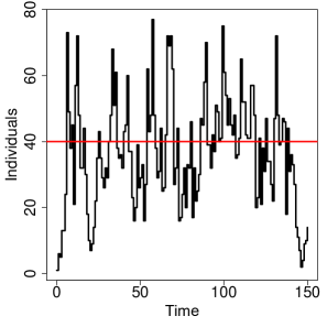
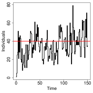
Figure 1: Evolution of the population sizes of two PSDBPs over the first 150 time units. Left: Beverton-Holt model. Right: Ricker model. Red solid line represents the carrying capacity.

Suppose that, based on the simulated trajectories, we would like to estimate the parameters $\boldsymbol{\theta}_{0}$. To this end we recall the MLE for $m(z,\boldsymbol{\theta})$, the mean number of offspring at population size $z$, derived in [2, Proposition 1]:

$$\hat{m}_{n}(z):=\frac{\sum_{i=0}^{n-1}Z_{i+1}\mathds{1}_{\{Z_{i}=z\}}}{z\,\sum_{i=0}^{n-1}\mathds{1}_{\{Z_{i}=z\}}},$$ (14)

where $\mathds{1}_{A}$ denotes the indicator function of the set $A$ and we take the convention that $0/0=0$. In Figure 2 we plot $m(z,\boldsymbol{\theta}_{0})$, $m^{\uparrow}(z,\boldsymbol{\theta}_{0})$ (defined in (10)), and the mean of $\hat{m}_{n}(z)$ for $n=5000$ over the 250 trajectories, for the Beverton-Holt and the Ricker models. Figure 2 illustrates that the outcomes of $\hat{m}_{n}(z)$ cling more tightly to the function $m^{\uparrow}(z,\boldsymbol{\theta}_{0})$ than to $m(z,\boldsymbol{\theta})$, which is due to the bias caused by restricting our attention to non-extinct trajectories. In particular [2, Theorem 1] states that, for any initial population size $i\in\mathbb{N}$ and population size $z\in\mathbb{N}$,

$$\forall\varepsilon>0,\quad\lim_{n\to\infty}\mathbb{P}_{i}[|\hat{m}_{n}(z)-m^{\uparrow}(z,\boldsymbol{\theta}_{0})|>\varepsilon|Z_{n}>0] =0\qquad\qquad\textrm{($Q$-consistency)}.$$ (15)

In Figure 2 we see that the functions $z\mapsto m^{\uparrow}(z,\boldsymbol{\theta}_{0})$ (red curve) and $z\mapsto m(z,\boldsymbol{\theta}_{0})$ (blue curve) are relatively close to each other at moderate and high population sizes ($z\geq 10$), however, they are significantly different at low population sizes. This motivates the weighted least squares estimators that we introduce in the next section.

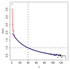
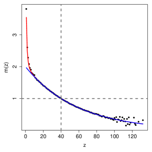
Figure 2: Means of $\hat{m}_{n}(z)$ (over the 250 processes) for each population size $z$ observed. Left: Beverton-Holt model. Right: Ricker model. The red solid curve represents the function $z\mapsto m^{\uparrow}(z,\boldsymbol{\theta}_{0})$ while the blue solid curve represents the function $z\mapsto m(z,\boldsymbol{\theta}_{0})$.

3 Weighted least squares estimators

In the context of branching processes, classical least squares estimators minimise the (weighted) squared differences between the population sizes $Z_{k}$ and their conditional mean $Z_{k-1}\,m(Z_{k-1},\boldsymbol{\theta})$, for $k=1,\ldots,n$:

$$\widetilde{\boldsymbol{\theta}}_{n}^{*}:=\arg\min_{\boldsymbol{\theta}\in\Theta}\sum_{k=1}^{n}w(Z_{k-1})\left\{Z_{k}-Z_{k-1}\,m(Z_{k-1},\boldsymbol{\theta})\right\}^{2},$$ (16)

where $w(\cdot)$ is an appropriately chosen weighting function (such as $w(Z_{k-1})=Z_{k-1}^{-1}$, see [8, p. 40]). This approach has been applied to Galton–Watson branching processes [8, Section 2.3], multi-type controlled branching processes [5], branching processes with immigration [13], and PSDBPs [14, 15]. Each of these papers develops asymptotic properties of $\widetilde{\boldsymbol{\theta}}_{n}^{*}$, such as consistency on the set of non-extinction, for processes with a positive chance of survival. Here we consider branching processes that become extinct almost surely, which introduces several technicalities that lead us to take a different approach.

To estimate $\boldsymbol{\theta}_{0}$ we develop a novel class of least squares estimators that use the $Q$-consistent estimators $\{\hat{m}_{n}(z)\}_{z\in\mathbb{N}}$, and that are $C$-consistent, that is, that satisfy (3). The idea is that, instead of summing over all time units $k=1,\ldots,n$ as in (16), we sum over all population sizes $z\geq 1$ and minimise the (weighted) squared differences between the MLE $\hat{m}_{n}(z)$ and its conditional limit ${m}^{\uparrow}(z,\boldsymbol{\theta})$:

$$\widehat{\boldsymbol{\theta}}_{n}:=\arg\min_{\theta\in\Theta}\sum_{z=1}^{\infty}\hat{w}_{n}(z)\left\{\hat{m}_{n}(z)-{m}^{\uparrow}(z,\boldsymbol{\theta})\right\}^{2},$$

where the weights $\{\hat{w}_{n}(z)\}_{z\in\mathbb{N}}$ are computed from the observations $Z_{0},Z_{1},\ldots,Z_{n}$. Estimators in this class can be viewed as hybrids between an MLE and a least squares estimator, where the MLEs $\{\hat{m}_{n}(z)\}_{z\in\mathbb{N}}$ first summarise the data before the least squares step is applied. In Figure 3 we give a visual representation of the classical least squares approach (top panel) and the hybrid approach taken in this paper (bottom panel).

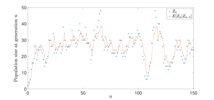
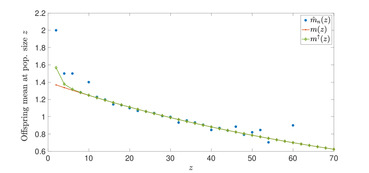
Figure 3: Top panel: the blue points correspond to a trajectory of $\{Z_{n}\}$ simulated from a PSDBP with carrying capacity $K=30$. The red curve represents the conditional expectation of $Z_{n}$ given the value of $Z_{n-1}$. This panel illustrates the differences $Z_{k}-Z_{k-1}\,m(Z_{k-1},\boldsymbol{\theta}_{0})=Z_{k}-\mathbb{E}(Z_{k}\,|\,Z_{k-1})$ in the classical least squares estimator $\widetilde{\boldsymbol{\theta}}_{n}^{*}$. Bottom panel: The trajectory of $Z_{n}$ is summarised in the values of $\{\hat{m}_{n}(z)\}_{z\geq 1}$ represented by the blue points. The green curve represents the function ${m}^{\uparrow}(z,\boldsymbol{\theta}_{0})$. This panel illustrates the differences $\hat{m}_{n}(z)-{m}^{\uparrow}(z,\boldsymbol{\theta})$ in the least squares estimator $\widehat{\boldsymbol{\theta}}_{n}$.

We suppose that the weights in (5) satisfy the following assumption:

1. For each $n\in\mathbb{N}$, $\{\hat{w}_{n}(z)\}$ is an empirical distribution (i.e., for each $z\in\mathbb{N}$, $\hat{w}_{n}(z)\geq 0$, and $\sum_{z\geq 1}\hat{w}_{n}(z)=1$), and there exists a limiting distribution $\{w_{z}\equiv w_{z}(\boldsymbol{\theta}_{0})\}_{z\in\mathbb{N}}$ such that, for any $i,z\geq 1$ and $\varepsilon>0$,

   $$\lim_{n\rightarrow\infty}\mathbb{P}_{i}[|\hat{w}_{n}(z)-w_{z}|>\varepsilon\,|\,Z_{n}>0]=0.$$

Two natural choices for the weight functions are

$$\hat{w}^{(1)}_{n}(z):=\frac{\sum_{i=0}^{n-1}\mathds{1}_{\{Z_{i}=z\}}}{n}\quad\text{ and }\quad\hat{w}^{(2)}_{n}(z):=\frac{z\sum_{i=0}^{n-1}\mathds{1}_{\{Z_{i}=z\}}}{\sum_{i=0}^{n-1}Z_{i}},$$ (17)

where $\hat{w}^{(1)}_{n}(z)$ assigns weights according to the proportion of time units with population size $z$, and $\hat{w}^{(2)}_{n}(z)$ assigns weights according to the proportion of parents alive when the population size is $z$.

Lemma 1.

The weights $\{\hat{w}^{(1)}_{n}(z)\}$ and $\{\hat{w}^{(2)}_{n}(z)\}$ satisfy Assumption (A1) with respective limiting distributions $\{w_{z}^{(1)}\}$ and $\{w_{z}^{(2)}\}$ characterised by

$${w}^{(1)}_{z}=u_{z}v_{z}\quad\text{ and }\quad{w}^{(2)}_{z}=\frac{zu_{z}v_{z}}{\sum_{k=1}^{\infty}ku_{k}v_{k}},\qquad z\in\mathbb{N}.$$

Note that $\{w_{z}^{(1)}\}$ is the stationary distribution of the $Q$-process $\{Z^{\uparrow}_{\ell}\}$, and $\{w_{z}^{(2)}\}$ is the size-biased distribution associated with $\{w_{z}^{(1)}\}$.

4 Asymptotic properties

We now establish that, under regularity assumptions, the class of least squares estimators $\widehat{\boldsymbol{\theta}}_{n}$ are $C$-consistent and asymptotically normal. We start by introducing some notation: let $\|\cdot\|$ denote any norm in $\mathbb{R}^{d}$ (recall that $\boldsymbol{\theta}$ is a $d$-dimensional parameter), let $\Psi_{\Sigma}(\cdot)$ denote the distribution function of a multivariate normal distribution with mean vector ${\boldsymbol{0}}=(0,\ldots,0)^{\top}$ and covariance matrix $\Sigma$ whose dimension will be clear from the context, and let $\nabla$ denote the gradient operator with respect to $\boldsymbol{\theta}$.

We make the following assumptions:

1. If $m^{\uparrow}(z,\boldsymbol{\theta}_{1})=m^{\uparrow}(z,\boldsymbol{\theta}_{2})$ for each $z\in\mathrm{supp}(\boldsymbol{w}(\boldsymbol{\theta}_{0}))$, then $\boldsymbol{\theta}_{1}=\boldsymbol{\theta}_{2}$.

2. $M:=\sup_{\boldsymbol{\theta}\in\Theta}\sup_{z\in\mathbb{N}}m^{\uparrow}(z,\boldsymbol{\theta})<\infty$.

3. For any initial state $i\in\mathbb{N}$, there exists $C>0$ such that

   $$\lim_{n\to\infty}\mathbb{P}_{i}\left[\sup_{z\in\mathbb{N}}|\hat{m}_{n}(z)-m^{\uparrow}(z,\boldsymbol{\theta}_{0})|<C\,\Big{|}\,Z_{n}>0\right]=1.$$

4. The function $m^{\uparrow}(z,\boldsymbol{\theta})$ is twice continuously differentiable with respect to $\boldsymbol{\theta}$ for each $z\in\mathbb{N}$. Moreover, for each $\boldsymbol{\theta}^{\prime}\in\Theta$, there exists a compact set $\mathcal{C}\equiv\mathcal{C}(\boldsymbol{\theta}^{\prime})$ such that $\boldsymbol{\theta}^{\prime}\in int(\mathcal{C})$ and

   1. $M_{1}^{*}(\boldsymbol{\theta}^{\prime}):=\sup_{\boldsymbol{\theta}\in\mathcal{C}}\sup_{z\in\mathbb{N}}\big{\|}\nabla m^{\uparrow}(z,\boldsymbol{\theta})\big{\|}_{\infty}<\infty$.

   2. $M_{2}^{*}(\boldsymbol{\theta}^{\prime}):=\sup_{\boldsymbol{\theta}\in\mathcal{C}}\sup_{z\in\mathbb{N}}\max_{i,j=1,\ldots,d}\left|\frac{\partial^{2}m^{\uparrow}(z,\boldsymbol{\theta})}{\partial\theta_{i}\partial\theta_{j}}\right|<\infty$.

   We comment on these assumptions in Remark 1 below.

Theorem 1 ($C$-consistency of $\widehat{\boldsymbol{\theta}}_{n}$).

Under Assumptions (A1)-(A4), for any $i\in\mathbb{N}$,

1. Existence:

   $$\lim_{n\to\infty}\mathbb{P}_{i}\left[\exists\,\widehat{\boldsymbol{\theta}}_{n}\,\big{|}\,Z_{n}>0\right]=1.$$

2. $C$-consistency:

   $$\forall\varepsilon>0,\quad\lim_{n\to\infty}\mathbb{P}_{i}\left[\big{\|}\widehat{\boldsymbol{\theta}}_{n}-\boldsymbol{\theta}_{0}\big{\|}>\varepsilon\,\big{|}\,Z_{n}>0\right]=0.$$

Theorem 2 ($C$-normality of $\widehat{\boldsymbol{\theta}}_{n}$).

Assume that either

• there exists a value $z^{*}<\infty$ such that for all $n\in\mathbb{N}$ and $z\geq z^{*}$, $\hat{w}_{n}(z)=0$, and Assumption (A1) holds; or

• for all $n\in\mathbb{N}$, $\{\hat{w}_{n}(z)\}=\{\hat{w}^{(1)}_{n}(z)\}$; or

• for all $n\in\mathbb{N}$, $\{\hat{w}_{n}(z)\}=\{\hat{w}^{(2)}_{n}(z)\}$.

Then, under Assumptions (A2)-(A5), for any $i\in\mathbb{N}$ and $x_{1},\ldots,x_{d}\in\mathbb{R}$,

$$\lim_{n\to\infty}\mathbb{P}_{i}\left[\sqrt{n}\left(\widehat{\boldsymbol{\theta}}_{n}-\boldsymbol{\theta}_{0}\right)\in(-\infty,x_{1}]\times\ldots\times(-\infty,x_{d}]\ \,\big{|}\,Z_{n}>0\right]=\Psi_{\beta(\boldsymbol{\theta}_{0})}(x_{1},\ldots,x_{d}),$$ (18)

where

$$\beta(\boldsymbol{\theta}_{0})=\eta(\boldsymbol{\theta}_{0})^{-1}\,\zeta(\boldsymbol{\theta}_{0})\,\eta(\boldsymbol{\theta}_{0})^{-1}$$

is a positive semi-definite matrix, with the $d$-dimensional matrices $\eta(\boldsymbol{\theta}_{0})$ and $\zeta(\boldsymbol{\theta}_{0})$ given by

$$\eta(\boldsymbol{\theta}_{0}) = 2\sum_{z=1}^{\infty}w_{z}(\boldsymbol{\theta}_{0})\,\nabla m^{\uparrow}(z,\boldsymbol{\theta}_{0})\nabla m^{\uparrow}(z,\boldsymbol{\theta}_{0})^{\top}$$

$$\zeta(\boldsymbol{\theta}_{0}) = 4\sum_{z=1}^{\infty}w_{z}(\boldsymbol{\theta}_{0})^{2}\,\gamma(z,\boldsymbol{\theta}_{0})\,\nabla m^{\uparrow}(z,\boldsymbol{\theta}_{0})\nabla m^{\uparrow}(z,\boldsymbol{\theta}_{0})^{\top},$$

where

$$\gamma(z,\boldsymbol{\theta}_{0}):=\frac{\sigma^{2\uparrow}(z,\boldsymbol{\theta}_{0})}{u_{z}(\boldsymbol{\theta}_{0})v_{z}(\boldsymbol{\theta}_{0})}.$$ (19)

Remark 1.

Assumption (A2) is expected to hold for a wide a variety of models including those considered in Section 2.3. Assumptions (A3) and (A4) hold if, for instance, the offspring distribution has bounded support, which is a reasonable assumption in most biological models. Assumption (A5) contains technical conditions that, in practice, would likely need to be verified numerically.

Remark 2.

Applying Theorem 2 with weights that satisfy (i) for a large value of $z^{*}$ should be sufficient in practice. Indeed, under Assumption 1-(C2), the process rarely takes very large values.

5 Simulated examples

In this section we compare the $C$-consistent estimator $\widehat{\boldsymbol{\theta}}_{n}$ (defined in (5)) with its natural counterpart obtained by replacing ${m}^{\uparrow}(z,\boldsymbol{\theta})$ with ${m}(z,\boldsymbol{\theta})$ in (5):

$$\widetilde{\boldsymbol{\theta}}_{n}:=\arg\min_{\theta\in\Theta}\sum_{z=1}^{\infty}\hat{w}_{n}(z)\left\{\hat{m}_{n}(z)-{m}(z,\boldsymbol{\theta})\right\}^{2}.$$ (20)

In general, due to (4), $\widetilde{\boldsymbol{\theta}}_{n}$ is not $C$-consistent when extinction is almost sure. In our examples, we consider the two weighting functions $\{\hat{w}^{(1)}_{n}(z)\}$ and $\{\hat{w}^{(2)}_{n}(z)\}$ defined in (17).

We separate our analysis into two cases: (i) populations which are still growing and are yet to reach the carrying capacity, and (ii) populations that start in the quasi-stationary regime (near the carrying capacity). We compare the accuracy of $\widehat{\boldsymbol{\theta}}_{n}$ and $\widetilde{\boldsymbol{\theta}}_{n}$ based on non-extinct trajectories.

5.1 Growing populations

Consider the illustrative example in Section 2.3 whose offspring distribution is given by (11), with $r(z,\boldsymbol{\theta})$ given by (12) (Beverton-Holt model) and where $\boldsymbol{b}(\mu)$ is a binary splitting distribution with $b_{2}=v$ and $b_{0}=1-v$ (so that $\mu=2v$). We fix the parameters $\boldsymbol{\theta}_{0}=(K_{0},v_{0})=(100,0.6)$ and the initial population size $N=2$, and simulate $N_{0}=2000$ trajectories of the process for $n=15,20,25$ time units such that $Z_{n}>0$. We estimate the parameters $\boldsymbol{\theta}_{0}$ based on the observed population sizes $z_{0},\ldots,z_{n}$. We are interested in comparing the performance of the estimators in the challenging —but practically important (see Section 6)— setting where the largest observation in most of the trajectories is well below the carrying capacity.

In Figure 4 we illustrate the sample mean of the $2000$ trajectories (left) and the histogram of the population size $Z_{25}$ of the simulated paths (right). We remark that the sample mean of $Z_{25}$ is well below the carrying capacity $K_{0}=100$ and its variance is large.

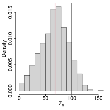
Figure 4: Beverton-Holt model with $(K_{0},v_{0})=(100,0.6)$. Left: Mean path of the 2000 simulated trajectories. Right: Histogram of $Z_{25}$; the red vertical line is the sample mean and the black vertical line is $K_{0}=100$.

	$n=15$				$n=20$				$n=25$
Method	Mean	Median	SD	RMSE	Mean	Median	SD	RMSE	Mean	Median	SD	RMSE
$\hat{K}_{n}(\boldsymbol{w_{n}^{(2)}})$	$77.175$	$46.611$	$83.466$	$0.748$	$90.148$	$70.348$	$74.418$	$0.563$	$97.458$	$86.029$	$62.931$	$0.396$
$\tilde{K}_{n}(\boldsymbol{w_{n}^{(2)}})$	$63.680$	$42.601$	$67.649$	$0.589$	$77.599$	$64.136$	$61.633$	$0.430$	$87.594$	$80.255$	$52.497$	$0.291$
$\hat{K}_{n}(\boldsymbol{w_{n}^{(1)}})$	$72.856$	$44.068$	$77.786$	$0.678$	$88.425$	$67.527$	$72.367$	$0.537$	$95.807$	$83.653$	$61.440$	$0.379$
$\tilde{K}_{n}(\boldsymbol{w_{n}^{(1)}})$	$46.036$	$35.035$	$43.451$	$0.480$	$58.220$	$51.476$	$40.160$	$0.336$	$67.530$	$66.104$	$32.094$	$0.208$
$\hat{v}_{n}(\boldsymbol{w_{n}^{(2)}})$	$0.646$	$0.647$	$0.076$	$0.022$	$0.639$	$0.637$	$0.059$	$0.014$	$0.632$	$0.633$	$0.052$	$0.010$
$\tilde{v}_{n}(\boldsymbol{w_{n}^{(2)}})$	$0.679$	$0.679$	$0.055$	$0.026$	$0.662$	$0.659$	$0.046$	$0.017$	$0.650$	$0.647$	$0.042$	$0.012$
$\hat{v}_{n}(\boldsymbol{w_{n}^{(1)}})$	$0.662$	$0.656$	$0.097$	$0.037$	$0.648$	$0.640$	$0.081$	$0.025$	$0.639$	$0.630$	$0.071$	$0.018$
$\tilde{v}_{n}(\boldsymbol{w_{n}^{(1)}})$	$0.734$	$0.730$	$0.070$	$0.064$	$0.713$	$0.705$	$0.062$	$0.046$	$0.697$	$0.687$	$0.057$	$0.035$

Table 1: Beverton-Holt model with $(K_{0},v_{0})=(100,0.6)$. Mean, median, standard deviation (SD) and relative mean squares error (RSME) of the estimates for $K_{0}$ and $v_{0}$ using the $C$-consistent estimator $\widehat{\boldsymbol{\theta}}_{n}=(\hat{K}_{n},\hat{v}_{n})$ in (5) and its counterpart $\widetilde{\boldsymbol{\theta}}_{n}=(\tilde{K}_{n},\tilde{v}_{n})$ in (20) with weighting functions $\{\hat{w}^{(1)}_{n}(z)\}$ and $\{\hat{w}^{(2)}_{n}(z)\}$ defined in (17), for $n=10,15,20$.

In Table 1, we provide the mean, median, standard deviation (SD) and relative mean squares error (RSME) of the estimates for $K_{0}$ and $v_{0}$ using the $C$-consistent estimator $\widehat{\boldsymbol{\theta}}_{n}=(\hat{K}_{n},\hat{v}_{n})$ in (5) and its counterpart $\widetilde{\boldsymbol{\theta}}_{n}=(\tilde{K}_{n},\tilde{v}_{n})$ in (20) with weighting functions $\{\hat{w}^{(1)}_{n}(z)\}$ and $\{\hat{w}^{(2)}_{n}(z)\}$ defined in (17), for $n=15,20,25$. First, we generally observe that, as expected, the estimates improve as $n$ increases. Second, we observe that the weighting function $\{\hat{w}^{(2)}_{n}(z)\}$ generally outperforms $\{\hat{w}^{(1)}_{n}(z)\}$; this is because the weights should ideally be equal to the inverse of the variance of the errors, and the limiting expression ${w}^{(2)}_{z}$ in Lemma 1 is (approximately) inversely proportional to $\gamma(z,\boldsymbol{\theta}_{0})$ in (19) which can be interpreted as the variance of the error $\{\hat{m}_{n}(z)-{m}^{\uparrow}(z,\boldsymbol{\theta})\}$ in the $z$th term of the least squares estimator $\widehat{\boldsymbol{\theta}}_{n}$ (see (32)).

More interestingly, for all $n$ and for both $K$ and $v$, the mean and median of $\widehat{\boldsymbol{\theta}}_{n}$ are closer to the true value $\boldsymbol{\theta}_{0}=(100,0.6)$ than the counterpart $\widetilde{\boldsymbol{\theta}}_{n}$ for any fixed weighting function; this illustrates that $\widehat{\boldsymbol{\theta}}_{n}$ has a smaller bias than $\widetilde{\boldsymbol{\theta}}_{n}$. The relative mean squares error is also always lower for $\hat{v}_{n}$ than for $\tilde{v}_{n}$. On the other hand, the standard deviation and relative mean squares error are smaller for $\tilde{K}_{n}$ than for $\hat{K}_{n}$. This is due to the presence of more outliers among the values of $\hat{K}_{n}$ than among those of $\tilde{K}_{n}$. In the left panel of Figure 5 we display the values of the difference $\hat{K}_{n}-\tilde{K}_{n}$; we see that these differences are generally positive, which decreases the overall bias of $\tilde{K}_{n}$ (recall that the median of $\tilde{K}_{25}(\boldsymbol{w_{n}^{(2)}})$ is 80.255), but there is a small chance that the difference is very large, which causes the standard deviation and relative mean squares error of $\hat{K}_{n}$ to be larger than those of $\tilde{K}_{n}$.

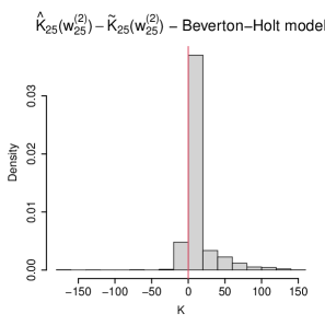
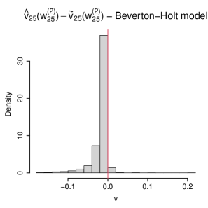
Figure 5: Beverton-Holt model with $(K_{0},v_{0})=(100,0.6)$. Marginal empirical distributions of the difference in the outcomes of the estimators $\widehat{\boldsymbol{\theta}}_{n}$ and $\widetilde{\boldsymbol{\theta}}_{n}$, with weighting function $\{\hat{w}^{(2)}_{n}(z)\}$ for the 2000 simulated trajectories, at $n=25$.

The box plots of $\widehat{\boldsymbol{\theta}}_{n}$ and $\widetilde{\boldsymbol{\theta}}_{n}$ with the weighting function $\{\hat{w}^{(2)}_{n}(z)\}$ and $\{\hat{w}^{(1)}_{n}(z)\}$ are illustrated in Figures 6 and 7, respectively. In these figures, we see that, for both $\{\hat{w}^{(2)}_{n}(z)\}$ and $\{\hat{w}^{(1)}_{n}(z)\}$, the true value of $K$ and $v$ generally lies between the first and third quantiles of the empirical distribution of $\widehat{\boldsymbol{\theta}}_{n}$, while this is not generally the case for $\widetilde{\boldsymbol{\theta}}_{n}$. In addition, we see that there is a bigger difference between $\widehat{\boldsymbol{\theta}}_{n}$ and $\widetilde{\boldsymbol{\theta}}_{n}$ for the weighting function $\{\hat{w}^{(1)}_{n}(z)\}$ than for $\{\hat{w}^{(2)}_{n}(z)\}$. This is because there are larger differences between $m(z)$ and $m^{\uparrow}(z)$ for small values of $z$ (recall Figure 2), and $\{\hat{w}^{(1)}_{n}(z)\}$ places more weight on small values of $z$ than $\{\hat{w}^{(2)}_{n}(z)\}$.

Finally, in Table 2 we present the estimates obtained when the 2000 trajectories are accumulated into a single sample, that is, we take

$$\hat{m}_{n}(z)=\frac{\sum_{j=1}^{2000}\sum_{i=0}^{n-1}Z_{j,i+1}\mathds{1}_{\{Z_{j,i}=z\}}}{z\,\sum_{j=1}^{2000}\sum_{i=0}^{n-1}\mathds{1}_{\{Z_{j,i}=z\}}},$$

where $Z_{j,i}$ is the population size at time $i$ in the $j$th trajectory, and we adjust the weighting functions $\{\hat{w}^{(2)}_{n}(z)\}$ and $\{\hat{w}^{(1)}_{n}(z)\}$ similarly. We observe that $\widehat{\boldsymbol{\theta}}_{n}$ significantly outperforms $\widetilde{\boldsymbol{\theta}}_{n}$ with both weighting functions. While the $C$-consistency of $\widehat{\boldsymbol{\theta}}_{n}$ stated in Theorem 1 ensures that ${m}^{\uparrow}(z,\boldsymbol{\theta})$ is the correct value to subtract in our least squares estimator for large values of $n$, Table 2 strongly suggests that this is also the case for relatively small values of $n$.

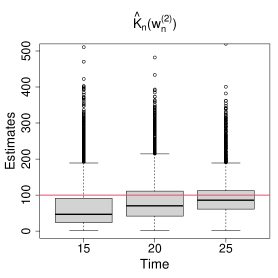
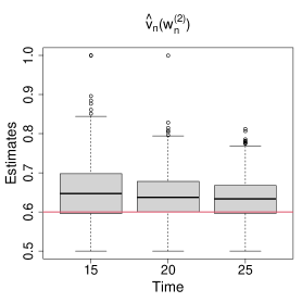
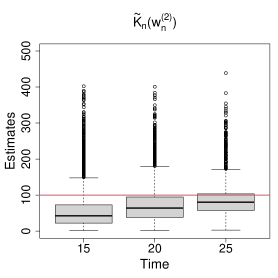
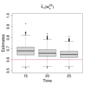
Figure 6: Beverton-Holt model with $(K_{0},v_{0})=(100,0.6)$. Box plots of $\widehat{\boldsymbol{\theta}}_{n}$ and $\widetilde{\boldsymbol{\theta}}_{n}$ with the weighting function $\{\hat{w}^{(2)}_{n}(z)\}$. Red lines represent the true value of each parameter.

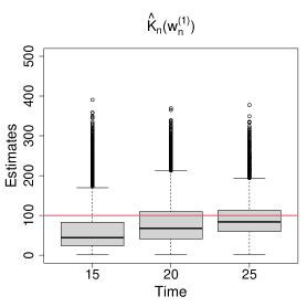
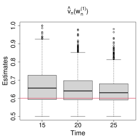
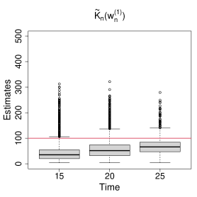
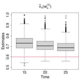
Figure 7: Beverton-Holt model with $(K_{0},v_{0})=(100,0.6)$. Box plots of $\widehat{\boldsymbol{\theta}}_{n}$ and $\widetilde{\boldsymbol{\theta}}_{n}$ with the weighting function $\{\hat{w}^{(1)}_{n}(z)\}$. Red lines represent the true value of each parameter.

	$n$
Method	$15$	$16$	$17$	$18$	$19$	$20$	$21$	$22$	$23$	$24$	$25$
$\hat{K}_{n}(\boldsymbol{w_{n}^{(1)}})$	$87.760$	$90.122$	$92.824$	$94.639$	$96.776$	$97.665$	$98.167$	$97.805$	$98.457$	$98.040$	$98.067$
$\tilde{K}_{n}(\boldsymbol{w_{n}^{(1)}})$	$45.730$	$49.477$	$53.353$	$56.905$	$60.421$	$63.525$	$66.340$	$68.613$	$71.073$	$72.981$	$74.810$
$\hat{K}_{n}(\boldsymbol{w_{n}^{(2)}})$	$91.781$	$94.270$	$97.384$	$99.505$	$100.856$	$101.601$	$101.296$	$100.737$	$101.186$	$100.437$	$100.302$
$\tilde{K}_{n}(\boldsymbol{w_{n}^{(2)}})$	$72.118$	$76.681$	$81.345$	$85.115$	$88.306$	$90.636$	$92.039$	$92.818$	$94.206$	$94.502$	$95.104$
$\hat{v}_{n}(\boldsymbol{w_{n}^{(1)}})$	$0.607$	$0.606$	$0.606$	$0.605$	$0.604$	$0.604$	$0.604$	$0.604$	$0.604$	$0.604$	$0.604$
$\tilde{v}_{n}(\boldsymbol{w_{n}^{(1)}})$	$0.687$	$0.682$	$0.678$	$0.674$	$0.671$	$0.668$	$0.666$	$0.664$	$0.662$	$0.660$	$0.659$
$\hat{v}_{n}(\boldsymbol{w_{n}^{(2)}})$	$0.604$	$0.604$	$0.603$	$0.602$	$0.601$	$0.601$	$0.601$	$0.601$	$0.601$	$0.601$	$0.601$
$\tilde{v}_{n}(\boldsymbol{w_{n}^{(2)}})$	$0.633$	$0.629$	$0.626$	$0.623$	$0.621$	$0.619$	$0.618$	$0.617$	$0.616$	$0.615$	$0.614$

Table 2: Beverton-Holt model with $(K_{0},v_{0})=(100,0.6)$. Estimates obtained when the 2000 trajectories are accumulated into a single sample.

5.2 Quasi-stationary populations

We consider the same Beverton-Holt model as in Section 5.1 and now focus on populations that linger around the carrying capacity. We fix $K_{0}=50$ and consider two scenarios, one where there are small fluctuations of $Z_{n}$ around the carrying capacity ($v_{0}=0.7$), and one where there are larger fluctuations ($v_{0}=0.54$). The amplitude of the fluctuations depends on the parameter $\mu=2v$ as follows: the larger the absolute value of the derivative of the mean offspring function $m(z)$ (assuming its support is extended to $\mathbb{R}_{+}$) at $z=K$, the smaller the fluctuations, as this derivative controls the strength of the drift toward $K$. For the Beverton-Holt model, $m^{\prime}(z)|_{z=k}=1-2v$, so taking $v_{0}=0.7$ leads to smaller fluctuations than $v_{0}=0.54$.

We fix the initial population size $N=2$ and simulate $N_{0}=2000$ trajectories of the process for $n=50,500,2000$ time units such that $Z_{n}>0$. In Figure 8 we plot the histogram of the population size $Z_{2000}$ based on the simulated trajectories for $v_{0}=0.7$ (left panel) and $v_{0}=0.54$ (right panel). The spread of the two histograms confirms that the population exhibits larger fluctuations around the carrying capacity when $v_{0}=0.54$ than when $v_{0}=0.7$.

We plot the histograms of the estimates for $K_{0}$ and $v_{0}$ and the confidence regions of their joint empirical distribution when $n=2000$ and $K_{0}=50$, for $v_{0}=0.7$ in Figure 9 and for $v_{0}=0.54$ in Figure 10. The blue curve plotted in the histograms for $\hat{K}$ and $\hat{v}$ is the density of the normal distribution with mean and variance computed using Theorem 2. The vertical blue lines give the boundaries of the resulting theoretical $95\%$ confidence intervals, and the vertical dashed lines give the boundaries of the empirical $95\%$ confidence intervals. In Tables 3 and 4 we provide the mean, median, standard deviation (SD) and relative mean square error (RMSE) of the estimates obtained with each of the estimators, for $v_{0}=0.7$ and $v_{0}=54$, respectively.

From both the figures and the tables, we observe that when $v_{0}=0.7$ (small fluctuations around the carrying capacity), the distributions of $\widehat{\boldsymbol{\theta}}_{n}$ and $\widetilde{\boldsymbol{\theta}}_{n}$ are similar across both weighting functions. In contrast, when $v_{0}=0.54$ (larger fluctuations around the carrying capacity), there is a visible difference between the distributions of $\widehat{\boldsymbol{\theta}}_{n}$ and $\widetilde{\boldsymbol{\theta}}_{n}$, and there is a clear bias in $\widetilde{\boldsymbol{\theta}}_{n}$. To understand why, recall that there is a larger difference between $m^{\uparrow}(z,\boldsymbol{\theta})$ and $m(z,\boldsymbol{\theta})$ for small values of $z$, and when $v_{0}=0.54$ there are larger fluctuations around the carrying capacity, which means that the process reaches these lower population sizes more frequently.

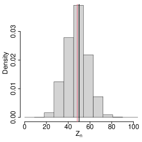
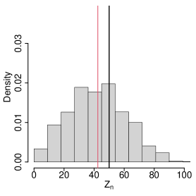
Figure 8: Beverton-Holt model. Left: Case with $(K_{0},v_{0})=(50,0.7)$. Right: Case with $(K_{0},v_{0})=(50,0.54)$. Red solid line is the mean population size at time $n=2000$ over the $2000$ simulated paths. Black solid line is the carrying capacity $K_{0}$.

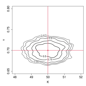
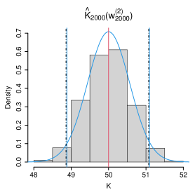
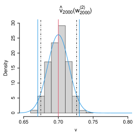
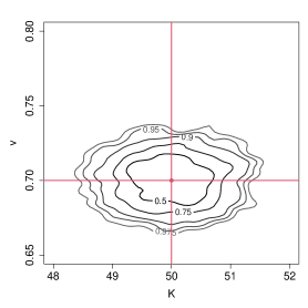
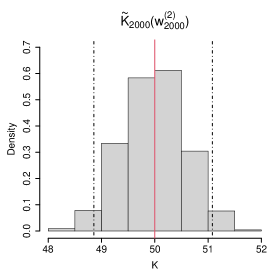
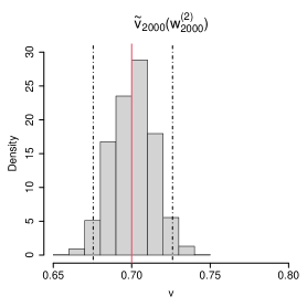
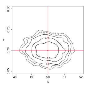
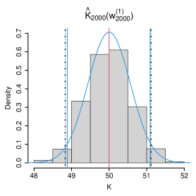
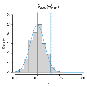
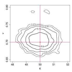
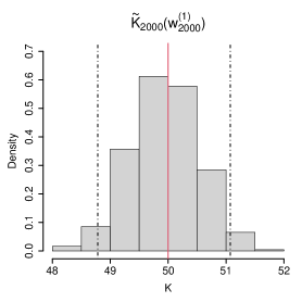
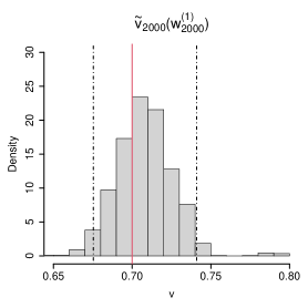
Figure 9: Case $(K_{0},v_{0})=(50,0.7)$. Left: confidence regions for levels $50\%,75\%,90\%,95\%,97.5\%$. Centre: marginal distribution of the estimator of $K$, together with the empirical and theoretical marginal 95% confidence intervals. Right: marginal distribution of the estimator of $v$, together with the empirical and theoretical marginal 95% confidence intervals.

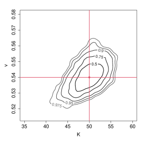
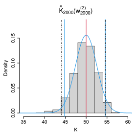
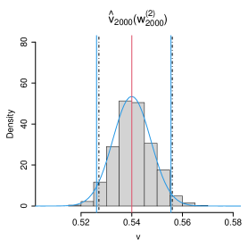
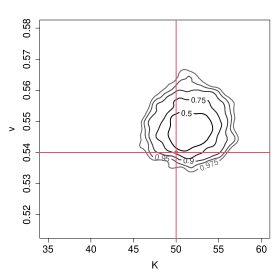
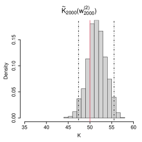
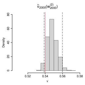
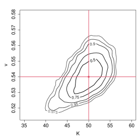
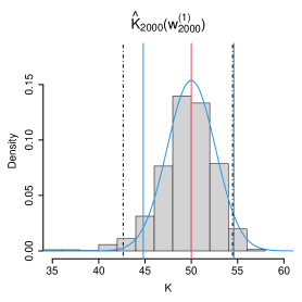
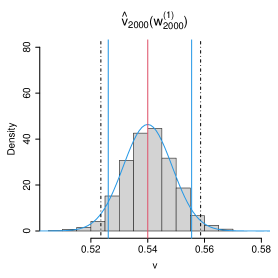
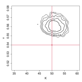
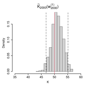
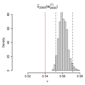
Figure 10: Case $(K_{0},v_{0})=(50,0.54)$. Left: confidence regions for levels $50\%,75\%,90\%,95\%,97.5\%$. Centre: marginal distribution of the estimator of $K$, together with the empirical and theoretical marginal 95% confidence intervals. Right: marginal distribution of the estimator of $v$, together with the empirical and theoretical marginal 95% confidence intervals.

		$\hat{K}_{n}(\boldsymbol{w_{n}^{(2)}})$	$\tilde{K}_{n}(\boldsymbol{w_{n}^{(2)}})$	$\hat{K}_{n}(\boldsymbol{w_{n}^{(1)}})$	$\tilde{K}_{n}(\boldsymbol{w_{n}^{(1)}})$	$\hat{v}_{n}(\boldsymbol{w_{n}^{(2)}})$	$\tilde{v}_{n}(\boldsymbol{w_{n}^{(2)}})$	$\hat{v}_{n}(\boldsymbol{w_{n}^{(1)}})$	$\tilde{v}_{n}(\boldsymbol{w_{n}^{(1)}})$
$n=50$	Median	$49.469$	$49.390$	$49.537$	$48.726$	$0.728$	$0.734$	$0.722$	$0.756$
	Mean	$49.399$	$49.332$	$49.362$	$48.766$	$0.734$	$0.741$	$0.735$	$0.768$
	SD	$4.159$	$4.138$	$5.338$	$4.295$	$0.068$	$0.065$	$0.093$	$0.082$
	RSME	$0.007$	$0.007$	$0.012$	$0.008$	$0.007$	$0.007$	$0.008$	$0.007$
$n=500$	Median	$50.007$	$50.005$	$49.978$	$49.841$	$0.704$	$0.706$	$0.706$	$0.725$
	Mean	$50.007$	$50.009$	$49.985$	$49.844$	$0.705$	$0.707$	$0.711$	$0.731$
	SD	$1.148$	$1.148$	$1.168$	$1.174$	$0.030$	$0.030$	$0.042$	$0.044$
	RSME	$0.001$	$0.001$	$0.001$	$0.001$	$0.002$	$0.002$	$0.004$	$0.006$
$n=2000$	Median	$49.999$	$49.997$	$49.998$	$49.954$	$0.701$	$0.701$	$0.701$	$0.708$
	Mean	$49.989$	$49.989$	$49.990$	$49.948$	$0.700$	$0.701$	$0.701$	$0.708$
	SD	$0.576$	$0.576$	$0.580$	$0.581$	$0.013$	$0.013$	$0.017$	$0.018$
	RSME	$0.0001$	$0.0001$	$0.0001$	$0.0001$	$0.0004$	$0.0004$	$0.001$	$0.001$

Table 3: Beverton-Holt model with $(K_{0},v_{0})=(50,0.7)$. Mean, median, standard deviation (SD) and relative mean square error (RMSE) of the estimates obtained with each of the estimators.

		$\hat{K}_{n}(\boldsymbol{w_{n}^{(2)}})$	$\tilde{K}_{n}(\boldsymbol{w_{n}^{(2)}})$	$\hat{K}_{n}(\boldsymbol{w_{n}^{(1)}})$	$\tilde{K}_{n}(\boldsymbol{w_{n}^{(1)}})$	$\hat{v}_{n}(\boldsymbol{w_{n}^{(2)}})$	$\tilde{v}_{n}(\boldsymbol{w_{n}^{(2)}})$	$\hat{v}_{n}(\boldsymbol{w_{n}^{(1)}})$	$\tilde{v}_{n}(\boldsymbol{w_{n}^{(1)}})$
$n=50$	Median	$40.528$	$40.787$	$38.777$	$36.647$	$0.577$	$0.602$	$0.583$	$0.655$
	Mean	$44.870$	$42.799$	$43.078$	$37.328$	$0.575$	$0.603$	$0.583$	$0.657$
	SD	$36.711$	$21.896$	$36.819$	$14.729$	$0.040$	$0.027$	$0.055$	$0.037$
	RMSE	$0.549$	$0.212$	$0.561$	$0.151$	$0.010$	$0.016$	$0.017$	$0.051$
$n=500$	Median	$49.454$	$51.329$	$49.292$	$50.315$	$0.544$	$0.552$	$0.545$	$0.575$
	Mean	$48.788$	$51.306$	$47.570$	$50.287$	$0.544$	$0.553$	$0.544$	$0.576$
	SD	$6.094$	$4.336$	$8.592$	$4.349$	$0.015$	$0.011$	$0.019$	$0.012$
	RMSE	$0.015$	$0.008$	$0.032$	$0.008$	$0.014$	$0.008$	$0.019$	$0.011$
$n=2000$	Median	$49.840$	$51.519$	$49.776$	$51.075$	$0.540$	$0.548$	$0.540$	$0.560$
	Mean	$49.707$	$51.531$	$49.518$	$51.076$	$0.541$	$0.548$	$0.541$	$0.561$
	SD	$2.685$	$2.086$	$3.001$	$2.120$	$0.008$	$0.006$	$0.009$	$0.005$
	RMSE	$0.003$	$0.003$	$0.004$	$0.002$	$0.0002$	$0.0003$	$0.0003$	$0.002$

Table 4: Beverton-Holt model with $(K_{0},v_{0})=(50,0.54)$. Mean, median, standard deviation (SD) and relative mean square error (RMSE) of the estimates obtained with each of the estimators.

The simulated examples in this section help us to form a general conclusion: if we are studying a population because it is still alive (i.e. under the condition $Z_{n}>0$) and the data contains observations of small population sizes ($<10$ individuals), then a $C$-consistent estimator such as $\widehat{\boldsymbol{\theta}}_{n}$ may be preferable to other similar estimators such as $\widetilde{\boldsymbol{\theta}}_{n}$. On the other hand, if there are no observations at small population sizes, then a $C$-consistent estimator such as $\widehat{\boldsymbol{\theta}}_{n}$ will generally be equivalent to other estimators such as $\widetilde{\boldsymbol{\theta}}_{n}$.

6 Application to the Chatham Island black robins

We now consider the real-world application of the Chatham Island black robins who breed seasonally and compete for territory, and for which a discrete-time PSDBP is therefore an appropriate model. We use a model slightly different from the one considered in Section 5, due to the characteristics of the population and the data which are available. The data consist of yearly nesting attempts, number of offspring when a nesting attempt is successful, and bird lifetimes between 1970 and 2000 ([3, 12]).

More precisely, individuals in our model are birds who are at least one-year old and able to reproduce. For every mother bird in year $n$, the following events are assumed to happen in this specific order between year $n$ and year $n+1$:

• the mother makes a successful attempt to reproduce with probability $r\equiv r(z,K,v)$ which depends on the current population size $z$, the carrying capacity $K$, and an ‘efficiency’ parameter $v$,

• if there is a successful reproduction attempt then the mother produces a random number of female birds who survive to the next year with distribution $\boldsymbol{b}=(b_{k})$, $k\geq 0$. The empirical distribution we obtained from the data is

  $$\boldsymbol{b}=[0.3130,0.4544,0.1758,0.0431,0.0106,0.0024,0.0006,0.0001],$$

  which is well approximated by a binomial distribution with parameters $n=5$ and $p=0.1988$ (fitted using the method of moments).

• the mother survives to the next year with probability $1-d=0.6861$ (estimated from the data), which we assume to be independent of the current population size and of whether she had a successful reproduction attempt.

Taking into account that, if the mother survives, then she is counted among her progeny, the effective offspring distribution is $\boldsymbol{p}=(p_{k})$, $k\geq 0$, with

$$p_{0} = (1-r)\,d+r\,b_{0}\,d$$

$$p_{1} = (1-r)\,(1-d)+r\,[b_{0}\,(1-d)+b_{1}\,d]$$

$$p_{k} = r\,[b_{k-1}\,(1-d)+b_{k}\,d],\quad k\geq 2.$$

We consider the Beverton-Holt and Ricker models where the probability $r$ of successful reproduction attempt is given by

$$r(z,K,v) = \dfrac{v\,K}{(\mu-1)z+K}\quad\textrm{(BH model)}$$

$$r(z,K,v) = v\,\left(\frac{1}{\mu}\right)^{\frac{z}{K}},\quad\textrm{(Ricker model)}$$

where the efficiency parameter $v$ is the probability of a successful reproduction attempt in the absence of competition, and $\mu:=5pv/d$. We estimate the two parameters $v$ and $K$ based on the yearly number of adult females between 1972 and 1998.

In Table 5 we present the estimates obtained with the estimators $\widehat{\boldsymbol{\theta}}_{n}$ and $\widetilde{\boldsymbol{\theta}}_{n}$ and the two weighting functions $\{\hat{w}^{(1)}_{n}(z)\}$ and $\{\hat{w}^{(2)}_{n}(z)\}$. In Figure 11 we plot the yearly population counts of the number of adult females and together with the mean population size curves of the Beverton Holt models and Ricker model estimated using weighting function $\{\hat{w}^{(2)}_{n}(z)\}$.

From Table 5 we see that, for both estimators $\widehat{\boldsymbol{\theta}}_{n}$ and $\widetilde{\boldsymbol{\theta}}_{n}$, there is a large difference in the estimates obtained using the two weighting functions. This is due to the fact that the number of breeding females was one for seven years in a row in the 1970’s (as can be seen in Figure 11), and the function $\{\hat{w}^{(1)}_{n}(z)\}$ places a significant amount of weight on these observations. As highlighted in Section 5.1, the weighting function $\{\hat{w}^{(1)}_{n}(z)\}$ does not generally provide results as accurate as the weighting function $\{\hat{w}^{(2)}_{n}(z)\}$, so here, we rely more on the results obtained with $\{\hat{w}^{(2)}_{n}(z)\}$.

We also observe from Table 5 that the estimates are quite sensitive to the chosen model. This is also highlighted in Figure 11, especially for the years after 1998 where the models are used for making predictions. The black robin population reached 239 adults in 2011 (that is, approximately 120 females) [18], so it appears that the Beverton-Holt model is more appropriate here than the Ricker model. Several other PSDBP models could be fitted to the black robin data, and a thorough model selection analysis should then be performed, in collaboration with experts in ecology.

	Beverton-Holt		Ricker
Method	$K$	$v$	$K$	$v$
$\hat{\boldsymbol{\theta}}_{n}(\boldsymbol{w_{n}^{(1)}})$	$256.8276$	$0.4492$	$242.1395$	$0.4521$
$\hat{\boldsymbol{\theta}}_{n}(\boldsymbol{w_{n}^{(2)}})$	$109.2115$	$0.6988$	$95.5616$	$0.6797$
$\tilde{\boldsymbol{\theta}}_{n}(\boldsymbol{w_{n}^{(1)}})$	$160.8160$	$0.5857$	$129.6446$	$0.5863$
$\tilde{\boldsymbol{\theta}}_{n}(\boldsymbol{w_{n}^{(2)}})$	$107.3594$	$0.7139$	$94.0594$	$0.6930$

Table 5: Black robin population. Estimates for the carrying capacity $K$ and the efficiency parameter $v$ obtained via each method.

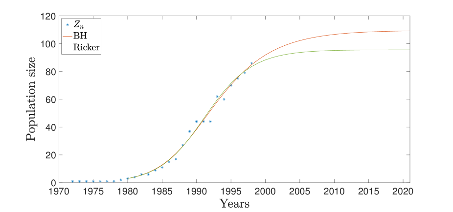
Figure 11: Black robin population. Number of adult females between 1972 and 1998 (blue points), together with the mean population size curve of the estimated Beverton Holt (red curve) and Ricker (green curve) models obtained with our estimator $\widehat{\boldsymbol{\theta}}_{n}$ and the weighting function .

7 Proofs

Proof of Lemma 1. The fact that $\hat{w}_{z}^{(1)}$ satisfies Assumption (A1) is a consequence of [7, Theorem 3(c)] (see also [2, Lemma 1]).

The fact that $\hat{w}_{z}^{(2)}$ satisfies Assumption (A1) follows from the fact that

$$\hat{w}^{(2)}_{n}(z)=\frac{z\sum_{i=0}^{n-1}\mathds{1}_{\{Z_{i}=z\}}}{\sum_{k=1}^{n}Z_{k}}=z\dfrac{\hat{w}_{z}^{(1)}}{\sum_{k=1}^{n}Z_{k}/n}.$$ (21)

Conditional on $Z_{n}>0$, the numerator of (21) converges in probability to $u_{z}v_{z}$, and the denominator converges to $\sum_{k=1}^{\infty}ku_{z}v_{z}$ in probability by [2, Lemma 6]. The result then follows from Slutsky’s theorem. ∎

To prove Theorems 1 and 2 we require the following two lemmas.

Lemma 2.

If the weights $\{\hat{w}_{n}(z)\}_{z\geq 1}$ satisfy Assumption (A1) then for each $\epsilon>0$,

$$\lim_{n\to\infty}\mathbb{P}_{i}\left[\sum_{z=1}^{\infty}\left|\hat{w}_{n}(z)-w_{z}\right|>\epsilon|Z_{n}>0\right]=0.$$

Proof of Lemma 2. First recall that $\{\hat{w}_{n}(z)\}$ and $\{w_{z}\}$ are probability distributions. Therefore, for any $\varepsilon>0$, we can choose $z^{*}(\varepsilon)$ such that

$$\sum_{z=z^{*}(\varepsilon)+1}^{\infty}w_{z}\leq\frac{\varepsilon}{4}.$$ (22)

Observe that if

$$|\hat{w}_{n}(z)-w_{z}|<\frac{\varepsilon}{4z^{*}(\varepsilon)},\quad\text{for all }z\in\{1,\dots,z^{*}(\varepsilon)\},$$ (23)

then

$$\sum_{z=1}^{\infty}|\hat{w}_{n}(z)-w_{z}| \leq\sum^{z^{*}(\varepsilon)}_{z=1}|\hat{w}_{n}(z)-w_{z}|+\sum^{\infty}_{z=z^{*}(\varepsilon)+1}w_{z}+\sum^{\infty}_{z=z^{*}(\varepsilon)+1}\hat{w}_{n}(z)$$

$$\leq\frac{\varepsilon}{4}+\frac{\varepsilon}{4}+1-\sum^{z^{*}(\varepsilon)}_{z=1}\hat{w}_{n}(z)$$

$$\leq\frac{\varepsilon}{2}+1-\sum^{z^{*}(\varepsilon)}_{z=1}w_{z}+\sum^{z^{*}(\varepsilon)}_{z=1}|\hat{w}_{n}(z)-w_{z}|$$

$$\leq\varepsilon,$$

where we have applied the triangle inequality, (22), (23), and the fact that $\{\hat{w}_{n}(z)\}$ is a probability distribution. Consequently,

$$\lim_{n\to\infty} \mathbb{P}_{i}\left[\sum_{z=1}^{\infty}\left|\hat{w}_{n}(z)-w_{z}\right|>\epsilon|Z_{n}>0\right]$$

$$\leq\lim_{n\to\infty}\mathbb{P}_{i}\left[\left|\hat{w}_{n}(z)-w_{z}\right|>\frac{\varepsilon}{4z^{*}(\varepsilon)},\text{ for some }z=1,\dots,z^{*}(\varepsilon)|Z_{n}>0\right]$$

$$\leq\sum_{i=1}^{z^{*}(\varepsilon)}\lim_{n\to\infty}\mathbb{P}_{i}\left[\left|\hat{w}_{n}(z)-w_{z}\right|>\frac{\varepsilon}{4z^{*}(\varepsilon)}|Z_{n}>0\right]$$

$$=0,$$

where in the final step we apply Assumption (A1).∎

Lemma 3.

Let $i\in\mathbb{N}$ be an initial state and $f:\boldsymbol{\theta}\in\Theta\mapsto[0,\infty)$ be a continuous function with a unique minimum at $\boldsymbol{\theta}_{0}$ that satisfies $f(\boldsymbol{\theta}_{0})=0$. For each $n\in\mathbb{N}$, let $f_{n}:(\omega,\boldsymbol{\theta})\in\Omega\times\Theta\mapsto\mathbb{R}_{+}$ be a function such that for each $\omega\in\Omega$, $f_{n}(\omega,\cdot)$ is a continuous function on $\Theta$, and for each $\boldsymbol{\theta}\in\Theta$, $f_{n}(\cdot,\boldsymbol{\theta})$ is a measurable function of the random variables $Z_{0},\ldots,Z_{n}$. If

$$\forall\epsilon>0,\quad\lim_{n\to\infty}\mathbb{P}_{i}\left[\omega\in\Omega:\sup_{\boldsymbol{\theta}\in\Theta}|f_{n}(\omega,\boldsymbol{\theta})-f(\boldsymbol{\theta})|>\epsilon|Z_{n}>0\right]=0,$$ (24)

then

1. $\lim_{n\to\infty}\mathbb{P}_{i}\left[\omega\in\Omega:\exists\arg\min_{\boldsymbol{\theta}\in\Theta}f_{n}(\omega,\boldsymbol{\theta})|Z_{n}>0\right]=1.$

2. $\forall\epsilon>0,\quad\lim_{n\to\infty}\mathbb{P}_{i}\left[\omega\in\Omega:\big{\|}\arg\min_{\boldsymbol{\theta}\in\Theta}f_{n}(\omega,\boldsymbol{\theta})-\boldsymbol{\theta}_{0}\big{\|}>\epsilon|Z_{n}>0\right]=0.$

Proof.

To ease the notation, throughout this proof let us denote $f_{n}(\boldsymbol{\theta})=f_{n}(\cdot,\boldsymbol{\theta})$. To establish (i) and (ii) we apply the following two identities that hold under (24): for any $\varepsilon>0$, and $C\subseteq\Theta$ we have

$$\lim_{n\to\infty}\mathbb{P}_{i}\left[f_{n}(\boldsymbol{\theta}_{0})>\epsilon|Z_{n}>0\right] =0,$$ (25)

$$\lim_{n\to\infty}\mathbb{P}_{i}\bigg{[}\big{|}\inf_{\boldsymbol{\theta}\in C}f_{n}(\boldsymbol{\theta})-\inf_{\boldsymbol{\theta}\in C}f(\boldsymbol{\theta})\big{|}>\epsilon|Z_{n}>0\bigg{]} =0.$$ (26)

To establish (25) we use the fact that, since $f(\boldsymbol{\theta}_{0})=0$, for any $n\in\mathbb{N}$ we have

$$\{\omega\in\Omega:f_{n}(\boldsymbol{\theta}_{0})>\varepsilon\}=\{\omega\in\Omega:|f_{n}(\boldsymbol{\theta}_{0})-f(\boldsymbol{\theta}_{0})|>\varepsilon\}\subseteq\{\omega\in\Omega:\sup_{\boldsymbol{\theta}\in\Theta}|f_{n}(\boldsymbol{\theta})-f(\boldsymbol{\theta})|>\varepsilon\},$$

which, by (24), implies

$$\lim_{n\to\infty}\mathbb{P}_{i}\bigg{[}f_{n}(\boldsymbol{\theta}_{0})>\epsilon|Z_{n}>0\bigg{]}\leq\lim_{n\to\infty}\mathbb{P}_{i}\bigg{[}\sup_{\boldsymbol{\theta}\in\Theta}\big{|}f_{n}(\boldsymbol{\theta})-f(\boldsymbol{\theta})\big{|}>\epsilon|Z_{n}>0\bigg{]}=0.$$

To establish (26), we denote $\boldsymbol{\theta}_{C}=\arg\inf_{\boldsymbol{\theta}\in C}f(\boldsymbol{\theta})$ and $\boldsymbol{\theta}_{n,C}=\arg\inf_{\boldsymbol{\theta}\in C}f_{n}(\boldsymbol{\theta})$. For any $\boldsymbol{\theta}^{\prime}\in C$ we have (surely)

$$\inf_{\boldsymbol{\theta}\in C}f_{n}(\boldsymbol{\theta})-\inf_{\boldsymbol{\theta}\in C}f(\boldsymbol{\theta})\leq f_{n}(\boldsymbol{\theta}^{\prime})-\inf_{\boldsymbol{\theta}\in C}f(\boldsymbol{\theta}),$$

and consequently,

$$\inf_{\boldsymbol{\theta}\in C}f_{n}(\boldsymbol{\theta})-\inf_{\boldsymbol{\theta}\in C}f(\boldsymbol{\theta})\leq f_{n}(\boldsymbol{\theta}_{C})-\inf_{\boldsymbol{\theta}\in C}f(\boldsymbol{\theta})=f_{n}(\boldsymbol{\theta}_{C})-f(\boldsymbol{\theta}_{C})\leq\sup_{\boldsymbol{\theta}\in\Theta}\big{|}f_{n}(\boldsymbol{\theta})-f(\boldsymbol{\theta})\big{|}.$$

Similarly,

$$\inf_{\boldsymbol{\theta}\in C}f(\boldsymbol{\theta})-\inf_{\boldsymbol{\theta}\in C}f_{n}(\boldsymbol{\theta})\leq f(\boldsymbol{\theta}_{n})-\inf_{\boldsymbol{\theta}\in C}f_{n}(\boldsymbol{\theta})=f(\boldsymbol{\theta}_{n})-f_{n}(\boldsymbol{\theta}_{n})\leq\sup_{\boldsymbol{\theta}\in\Theta}\big{|}f_{n}(\boldsymbol{\theta})-f(\boldsymbol{\theta})\big{|}.$$

Combining both the above inequalities we see that for any $n\in\mathbb{N}$ and $\epsilon>0$,

$$\bigg{\{}\big{|}\inf_{\boldsymbol{\theta}\in C}f_{n}(\boldsymbol{\theta})-\inf_{\boldsymbol{\theta}\in C}f(\boldsymbol{\theta})\big{|}>\epsilon\bigg{\}}\subseteq\bigg{\{}\sup_{\boldsymbol{\theta}\in\Theta}\big{|}f_{n}(\boldsymbol{\theta})-f(\boldsymbol{\theta})\big{|}>\epsilon\bigg{\}},$$

which then allows us to apply (24) to obtain (26).

To establish (i) we observe that it is sufficient to show that, for any compact set $C\subset\Theta$ with $\boldsymbol{\theta}_{0}\in C$, we have

$$\lim_{n\to\infty}\mathbb{P}_{i}\bigg{[}\inf_{\boldsymbol{\theta}\in\Theta\backslash C}f_{n}(\boldsymbol{\theta})>\min_{\boldsymbol{\theta}\in C}f_{n}(\boldsymbol{\theta})|Z_{n}>0\bigg{]}=1.$$ (27)

Note that, because $C$ is a compact set, and because for any $n\in\mathbb{N}$ and $\omega\in\Omega$, $\boldsymbol{\theta}\mapsto f_{n}(\omega,\boldsymbol{\theta})$ is a continuous function on $\Theta$, $\min_{\boldsymbol{\theta}\in C}f_{n}(\boldsymbol{\theta})$ exists. The claim in (i) then follows from (27) by letting $C$ be an arbitrarily small closed ball centered at $\boldsymbol{\theta}_{0}$.

To establish (27) we let $0<\varepsilon=a/4$, with $a=\inf_{\boldsymbol{\theta}\in\Theta\backslash C}f(\boldsymbol{\theta})>0$, and observe that

$$\bigg{\{}f_{n}(\boldsymbol{\theta}_{0})\leq\epsilon\bigg{\}}\cap\bigg{\{}\Big{|}\inf_{\boldsymbol{\theta}\in\Theta\backslash C}f_{n}(\boldsymbol{\theta})-a\Big{|}\leq\epsilon\bigg{\}}\subseteq\bigg{\{}\min_{\boldsymbol{\theta}\in C}f_{n}(\boldsymbol{\theta})\leq f_{n}(\boldsymbol{\theta}_{0})\leq\frac{a}{4}<\frac{3a}{4}\leq\inf_{\boldsymbol{\theta}\in\Theta\backslash C}f_{n}(\boldsymbol{\theta})\bigg{\}}.$$

We then apply (25) and (26) to obtain (27).

To establish (ii) we let $\boldsymbol{\vartheta}_{n}=\arg\min_{\boldsymbol{\theta}\in\Theta}f_{n}(\boldsymbol{\theta})$, and use the fact that

$$\forall\epsilon>0,\quad\lim_{n\to\infty}\mathbb{P}_{i}\left[f(\boldsymbol{\vartheta}_{n})>\epsilon|Z_{n}>0\right]=0.$$ (28)

Indeed, (28) follows by applying both (26) with $C=\Theta$, to obtain

$$\forall\epsilon>0,\quad\lim_{n\to\infty}\mathbb{P}_{i}\left[f_{n}(\boldsymbol{\vartheta}_{n})>\epsilon|Z_{n}>0\right]=0,$$

and (24) to obtain

$$\forall\epsilon>0,\quad\lim_{n\to\infty}\mathbb{P}_{i}\Big{[}\big{|}f_{n}(\boldsymbol{\vartheta}_{n})-f(\boldsymbol{\vartheta}_{n})\big{|}>\epsilon|Z_{n}>0\Big{]}=0.$$

To prove (ii), we then note that, for each $\varepsilon>0$, given that $f(\cdot)$ has a unique minimum at $\boldsymbol{\theta}_{0}$, we can take $C=\{\boldsymbol{\theta}\in\Theta:\|\boldsymbol{\theta}-\boldsymbol{\theta}_{0}\|\leq\varepsilon\}$, $b=\inf_{\Theta\backslash C}f(\boldsymbol{\theta})$, and $\beta=b/2$; then $0=\min_{\boldsymbol{\theta}\in C}f(\boldsymbol{\theta})<\beta<b$. Moreover, we have $b=\inf_{\Theta\backslash C}f(\boldsymbol{\theta})\leq f(\boldsymbol{\theta}^{\prime})$ for every $\boldsymbol{\theta}^{\prime}\in\Theta\backslash C$, and consequently

$$\{\|\boldsymbol{\vartheta}_{n}-\boldsymbol{\theta}_{0}\|>\varepsilon\}\subseteq\{f(\boldsymbol{\vartheta}_{n})>\beta\}.$$

The result in (ii) now follows from (28). ∎

We are now ready to establish the limiting properties of the estimator $\widehat{\boldsymbol{\theta}}_{n}$, namely, $C$-consistency (Theorem 1) and $C$-normality (Theorem 2). For each $n\in\mathbb{N}$, recall that

$$\widehat{\boldsymbol{\theta}}_{n}=\arg\min_{\boldsymbol{\theta}\in\Theta}S_{n}(\boldsymbol{\theta}),\qquad\textrm{where}\qquad S_{n}(\boldsymbol{\theta}):=\sum_{z=1}^{\infty}\hat{w}_{n}(z)(m^{\uparrow}(z,\boldsymbol{\theta})-\hat{m}_{n}(z))^{2}.$$

Proof of Theorem 1

Let us fix $i\in\mathbb{N}$. By Lemma 3, it is enough to prove that

$$\forall\epsilon>0,\quad\lim_{n\to\infty}\mathbb{P}_{i}\left[\sup_{\boldsymbol{\theta}\in\Theta}\left|S_{n}(\boldsymbol{\theta})-S(\boldsymbol{\theta})\right|>\epsilon|Z_{n}>0\right]=0,$$

where

$$S(\boldsymbol{\theta}):=\sum_{z=1}^{\infty}w_{z}(\boldsymbol{\theta}_{0})(m^{\uparrow}(z,\boldsymbol{\theta})-m^{\uparrow}(z,\boldsymbol{\theta}_{0}))^{2}.$$

To that end, we introduce the following function

$$\hat{S}_{n}(\boldsymbol{\theta})=\sum_{z=1}^{\infty}w_{z}(\boldsymbol{\theta}_{0})\mathds{1}_{\{j_{n}(z)>0\}}(m^{\uparrow}(z,\boldsymbol{\theta})-\hat{m}_{n}(z))^{2},\quad n\in\mathbb{N},\ \boldsymbol{\theta}\in\Theta,$$

where $j_{n}(z):=\sum_{i=0}^{n-1}\mathds{1}_{\{Z_{i}=z\}}$. It then suffices to prove that, for each $\epsilon>0$,

1. $\lim_{n\to\infty}\mathbb{P}_{i}\left[\sup_{\boldsymbol{\theta}\in\Theta}\left|S_{n}(\boldsymbol{\theta})-\hat{S}_{n}(\boldsymbol{\theta})\right|>\epsilon|Z_{n}>0\right]=0$,

2. $\lim_{n\to\infty}\mathbb{P}_{i}\left[\sup_{\boldsymbol{\theta}\in\Theta}\left|\hat{S}_{n}(\boldsymbol{\theta})-S(\boldsymbol{\theta})\right|>\epsilon|Z_{n}>0\right]=0$.

We start with the proof of (a). Recall the definition of $M$ and $C$ from Assumptions (A3) and (A4), respectively. Let $M^{\prime}=2(M+C)^{2}$ and $A_{n}=\sup_{z\in\mathbb{N}}|m^{\uparrow}(z,\boldsymbol{\theta}_{0})-\hat{m}_{n}(z)|$. On the set $\{A_{n}\leq C\}$ we have

$$\sup_{\boldsymbol{\theta}\in\Theta}|S_{n}(\boldsymbol{\theta}) -\hat{S}_{n}(\boldsymbol{\theta})|\leq\sup_{\boldsymbol{\theta}\in\Theta}\sum_{z=1}^{\infty}|\hat{w}_{n}(z)-w_{z}(\boldsymbol{\theta}_{0})\mathds{1}_{\{j_{n}(z)>0\}}|(m^{\uparrow}(z,\boldsymbol{\theta})-\hat{m}_{n}(z))^{2}$$

$$=\sup_{\boldsymbol{\theta}\in\Theta}\sum_{z=1}^{\infty}|\hat{w}_{n}(z)-w_{z}(\boldsymbol{\theta}_{0})\mathds{1}_{\{j_{n}(z)>0\}}|(m^{\uparrow}(z,\boldsymbol{\theta})-m^{\uparrow}(z,\boldsymbol{\theta}_{0})+m^{\uparrow}(z,\boldsymbol{\theta}_{0})-\hat{m}_{n}(z))^{2}$$

$$\leq\sup_{\boldsymbol{\theta}\in\Theta}\sum_{z=1}^{\infty}|\hat{w}_{n}(z)-w_{z}(\boldsymbol{\theta}_{0})\mathds{1}_{\{j_{n}(z)>0\}}|(m^{\uparrow}(z,\boldsymbol{\theta})-m^{\uparrow}(z,\boldsymbol{\theta}_{0}))^{2}$$

$$\phantom{=}+\sum_{z=1}^{\infty}|\hat{w}_{n}(z)-w_{z}(\boldsymbol{\theta}_{0})\mathds{1}_{\{j_{n}(z)>0\}}|(m^{\uparrow}(z,\boldsymbol{\theta}_{0})-\hat{m}_{n}(z))^{2}$$

$$\phantom{=}+2\sup_{\boldsymbol{\theta}\in\Theta}\sum_{z=1}^{\infty}|\hat{w}_{n}(z)-w_{z}(\boldsymbol{\theta}_{0})\mathds{1}_{\{j_{n}(z)>0\}}|\cdot|m^{\uparrow}(z,\boldsymbol{\theta})-m^{\uparrow}(z,\boldsymbol{\theta}_{0})|\cdot|m^{\uparrow}(z,\boldsymbol{\theta}_{0})-\hat{m}_{n}(z)|$$

$$\leq M^{\prime}\sum_{z=1}^{\infty}|\hat{w}_{n}(z)-w_{z}(\boldsymbol{\theta}_{0})\mathds{1}_{\{j_{n}(z)>0\}}|$$

$$\leq M^{\prime}\sum_{z=1}^{\infty}|\hat{w}_{n}(z)-w_{z}(\boldsymbol{\theta}_{0})+w_{z}(\boldsymbol{\theta}_{0})-w_{z}(\boldsymbol{\theta}_{0})\mathds{1}_{\{j_{n}(z)>0\}}|$$

$$\leq M^{\prime}\sum_{z=1}^{\infty}|\hat{w}_{n}(z)-w_{z}(\boldsymbol{\theta}_{0})|+M^{\prime}\sum_{z=1}^{\infty}w_{z}(\boldsymbol{\theta}_{0})\mathds{1}_{\{j_{n}(z)=0\}}.$$

Consequently,

$$\left\{\sup_{\boldsymbol{\theta}\in\Theta}|S_{n}(\boldsymbol{\theta})-\hat{S}_{n}(\boldsymbol{\theta})|>\epsilon\right\} =\left\{\sup_{\boldsymbol{\theta}\in\Theta}|S_{n}(\boldsymbol{\theta})-\hat{S}_{n}(\boldsymbol{\theta})|>\epsilon,A_{n}\leq C\right\}\cup$$

$$\phantom{=}\cup\left\{\sup_{\boldsymbol{\theta}\in\Theta}|S_{n}(\boldsymbol{\theta})-\hat{S}_{n}(\boldsymbol{\theta})|>\epsilon,A_{n}>C\right\}$$

$$\subseteq\left\{\sum_{z=1}^{\infty}|\hat{w}_{n}(z)-w_{z}(\boldsymbol{\theta}_{0})|>\frac{\epsilon}{2M^{\prime}},A_{n}\leq C\right\}\cup$$

$$\phantom{=}\cup\left\{\sum_{z=1}^{\infty}w_{z}(\boldsymbol{\theta}_{0})\mathds{1}_{\{j_{n}(z)=0\}}>\frac{\epsilon}{2M^{\prime}},A_{n}\leq C\right\}\cup\left\{A_{n}>C\right\}$$

$$\subseteq\left\{\sum_{z=1}^{\infty}|\hat{w}_{n}(z)-w_{z}(\boldsymbol{\theta}_{0})|>\frac{\epsilon}{2M^{\prime}}\right\}\cup\left\{\sum_{z=1}^{\infty}w_{z}(\boldsymbol{\theta}_{0})\mathds{1}_{\{j_{n}(z)=0\}}>\frac{\epsilon}{2M^{\prime}}\right\}$$

$$\phantom{=}\cup\left\{A_{n}>C\right\}.$$

Conditioning on $Z_{n}>0$, we then obtain (a) by applying Lemma 2 to the first event, the fact that $\lim_{n\to\infty}\mathbb{P}[\mathds{1}_{\{j_{n}(z)=0\}}\leq\epsilon|Z_{n}>0]=1$ for any $\epsilon>0,z\in\mathbb{N}$ and that $\sum_{z=1}^{\infty}w_{z}(\boldsymbol{\theta}_{0})=1$ to the second event, and Assumption (A4) to the third event.

In order to prove (b), we observe that

$$\hat{S}_{n}(\boldsymbol{\theta})-S(\boldsymbol{\theta}) =\sum_{z=1}^{\infty}w_{z}(\boldsymbol{\theta}_{0})\mathds{1}_{\{j_{n}(z)>0\}}\left[(m^{\uparrow}(z,\boldsymbol{\theta})-\hat{m}_{n}(z))^{2}-(m^{\uparrow}(z,\boldsymbol{\theta})-m^{\uparrow}(z,\boldsymbol{\theta}_{0}))^{2}\right]$$

$$\phantom{=}-\sum_{z=1}^{\infty}w_{z}(\boldsymbol{\theta}_{0})\mathds{1}_{\{j_{n}(z)=0\}}(m^{\uparrow}(z,\boldsymbol{\theta})-m^{\uparrow}(z,\boldsymbol{\theta}_{0}))^{2}$$

$$=\sum_{z=1}^{\infty}w_{z}(\boldsymbol{\theta}_{0})\mathds{1}_{\{j_{n}(z)>0\}}\left[\hat{m}_{n}(z)^{2}-2\hat{m}_{n}(z)m^{\uparrow}(z,\boldsymbol{\theta})-m^{\uparrow}(z,\boldsymbol{\theta}_{0})^{2}+2m^{\uparrow}(z,\boldsymbol{\theta})m^{\uparrow}(z,\boldsymbol{\theta}_{0})\right]$$

$$\phantom{=}-\sum_{z=1}^{\infty}w_{z}(\boldsymbol{\theta}_{0})\mathds{1}_{\{j_{n}(z)=0\}}(m^{\uparrow}(z,\boldsymbol{\theta})-m^{\uparrow}(z,\boldsymbol{\theta}_{0}))^{2},$$

then

$$\sup_{\boldsymbol{\theta}\in\Theta}|\hat{S}_{n}(\boldsymbol{\theta})-S(\boldsymbol{\theta})| \leq\sum_{z=1}^{\infty}w_{z}(\boldsymbol{\theta}_{0})\mathds{1}_{\{j_{n}(z)>0\}}\left|\hat{m}_{n}(z)^{2}-m^{\uparrow}(z,\boldsymbol{\theta}_{0})^{2}\right|$$

$$\phantom{=}+2\sup_{\boldsymbol{\theta}\in\Theta}\sum_{z=1}^{\infty}w_{z}(\boldsymbol{\theta}_{0})\mathds{1}_{\{j_{n}(z)>0\}}m^{\uparrow}(z,\boldsymbol{\theta})\left|\hat{m}_{n}(z)-m^{\uparrow}(z,\boldsymbol{\theta}_{0})\right|$$

$$\phantom{=}+\sup_{\boldsymbol{\theta}\in\Theta}\sum_{z=1}^{\infty}w_{z}(\boldsymbol{\theta}_{0})\mathds{1}_{\{j_{n}(z)=0\}}(m^{\uparrow}(z,\boldsymbol{\theta})-m^{\uparrow}(z,\boldsymbol{\theta}_{0}))^{2},$$

and consequently,

$$\left\{\sup_{\boldsymbol{\theta}\in\Theta}|\hat{S}_{n}(\boldsymbol{\theta})-S(\boldsymbol{\theta})|>\epsilon\right\} \subseteq\left\{\sum_{z=1}^{\infty}w_{z}(\boldsymbol{\theta}_{0})\mathds{1}_{\{j_{n}(z)>0\}}\left|\hat{m}_{n}(z)^{2}-m^{\uparrow}(z,\boldsymbol{\theta}_{0})^{2}\right|>\frac{\epsilon}{3}\right\}\cup$$ (29)

$$\phantom{\subseteq}\cup\left\{\sup_{\boldsymbol{\theta}\in\Theta}\sum_{z=1}^{\infty}w_{z}(\boldsymbol{\theta}_{0})\mathds{1}_{\{j_{n}(z)>0\}}m^{\uparrow}(z,\boldsymbol{\theta})\left|\hat{m}_{n}(z)-m^{\uparrow}(z,\boldsymbol{\theta}_{0})\right|>\frac{\epsilon}{6}\right\}$$ (30)

$$\phantom{\subseteq}\cup\left\{\sup_{\boldsymbol{\theta}\in\Theta}\sum_{z=1}^{\infty}w_{z}(\boldsymbol{\theta}_{0})\mathds{1}_{\{j_{n}(z)=0\}}(m^{\uparrow}(z,\boldsymbol{\theta})-m^{\uparrow}(z,\boldsymbol{\theta}_{0}))^{2}>\frac{\epsilon}{3}\right\}$$ (31)

Because $\mathbb{P}_{i}(A_{n}>C|Z_{n}>0)\to 0$ by (A4), we can restrict our attention to the set $\{A_{n}\leq C\}$. On the set $\{A_{n}\leq C\}$,

$$\sup_{z\in\mathbb{N}}\left|\hat{m}_{n}(z)^{2}-m^{\uparrow}(z,\boldsymbol{\theta}_{0})^{2}\right| \leq\sup_{z\in\mathbb{N}}\left|\hat{m}_{n}(z)-m^{\uparrow}(z,\boldsymbol{\theta}_{0})\right|\cdot\sup_{z\in\mathbb{N}}\left|\hat{m}_{n}(z)+m^{\uparrow}(z,\boldsymbol{\theta}_{0})\right|$$

$$\leq C(C+2M)\leq M^{\prime}.$$

In addition, since ${\boldsymbol{w}}(\boldsymbol{\theta}_{0})$ is a probability distribution, given $\epsilon>0$, there exists $K_{0}=K_{0}(\epsilon)\in\mathbb{N}$ such that $\sum_{z=K_{0}+1}^{\infty}w_{z}(\boldsymbol{\theta}_{0})<\frac{\epsilon}{6M^{\prime}}$. Consequently, on $\{A_{n}\leq C\}$

$$\sum_{z=1}^{\infty}w_{z}(\boldsymbol{\theta}_{0})\mathds{1}_{\{j_{n}(z)>0\}}\left|\hat{m}_{n}(z)^{2}-m^{\uparrow}(z,\boldsymbol{\theta}_{0})^{2}\right| \leq\sum_{z=1}^{K_{0}}w_{z}(\boldsymbol{\theta}_{0})\mathds{1}_{\{j_{n}(z)>0\}}\left|\hat{m}_{n}(z)^{2}-m^{\uparrow}(z,\boldsymbol{\theta}_{0})^{2}\right|$$

$$\phantom{=}+M^{\prime}\sum_{z=K_{0}+1}^{\infty}w_{z}(\boldsymbol{\theta}_{0}),$$

and hence

$$\bigcap_{z=1}^{K_{0}}\bigg{\{}w_{z}(\boldsymbol{\theta}_{0})\mathds{1}_{\{j_{n}(z)>0\}} \left|\hat{m}_{n}(z)^{2}-m^{\uparrow}(z,\boldsymbol{\theta}_{0})^{2}\right|\leq\frac{\epsilon}{6K_{0}}\bigg{\}}\bigcap\{A_{n}\leq C\}\subseteq$$

$$\subseteq\Big{\{}\sum_{z=1}^{\infty}w_{z}(\boldsymbol{\theta}_{0})\mathds{1}_{\{j_{n}(z)>0\}}\left|\hat{m}_{n}(z)^{2}-m^{\uparrow}(z,\boldsymbol{\theta}_{0})^{2}\right|\leq\frac{\epsilon}{3}\Big{\}}\bigcap\{A_{n}\leq C\}.$$

Thus, by (15), we get that

$$\lim_{n\to\infty}\mathbb{P}_{i}\bigg{[}\Big{\{}\sum_{z=1}^{\infty}w_{z}(\boldsymbol{\theta}_{0})\mathds{1}_{\{j_{n}(z)>0\}}\left|\hat{m}_{n}(z)^{2}-m^{\uparrow}(z,\boldsymbol{\theta}_{0})^{2}\right|\leq\frac{\epsilon}{3}\Big{\}}\cap\{A_{n}\leq C\}|Z_{n}>0\bigg{]}=1,$$

and then

$$\lim_{n\to\infty}\mathbb{P}_{i}\bigg{[}\sum_{z=1}^{\infty}w_{z}(\boldsymbol{\theta}_{0})\mathds{1}_{\{j_{n}(z)>0\}}\left|\hat{m}_{n}(z)^{2}-m^{\uparrow}(z,\boldsymbol{\theta}_{0})^{2}\right|\leq\frac{\epsilon}{3}|Z_{n}>0\bigg{]}=1.$$

With similar arguments using $\sup_{\boldsymbol{\theta}\in\Theta}\sup_{z\in\mathbb{N}}\left(m^{\uparrow}(z,\boldsymbol{\theta})-m^{\uparrow}(z,\boldsymbol{\theta}_{0})\right)^{2}\leq 4M^{2}$, and we obtain

$$\lim_{n\to\infty}\mathbb{P}_{i}\bigg{[}\sup_{\boldsymbol{\theta}\in\Theta}\sum_{z=1}^{\infty}w_{z}(\boldsymbol{\theta}_{0})\mathds{1}_{\{j_{n}(z)>0\}}m^{\uparrow}(z,\boldsymbol{\theta})\left|\hat{m}_{n}(z)-m^{\uparrow}(z,\boldsymbol{\theta}_{0})\right|\leq\frac{\epsilon}{6}|Z_{n}>0\bigg{]}=1,$$

$$\lim_{n\to\infty}\mathbb{P}_{i}\bigg{[}\sup_{\boldsymbol{\theta}\in\Theta}\sum_{z=1}^{\infty}w_{z}(\boldsymbol{\theta}_{0})\mathds{1}_{\{j_{n}(z)=0\}}(m^{\uparrow}(z,\boldsymbol{\theta})-m^{\uparrow}(z,\boldsymbol{\theta}_{0}))^{2}\leq\frac{\epsilon}{3}|Z_{n}>0\bigg{]}=1.$$

Consequently we have proved (b) and the result now follows.

$\Box$

Before we prove Theorem 2 we recall the asymptotic normality of the MLEs $\{\hat{m}_{n}(z)\}_{z\in\mathbb{N}}$ that is established in [2, Theorem 1]: for any $i,z,z_{1},z_{2}\in\mathbb{N}$ and $x,x_{1},x_{2}\in\mathbb{R}$,

$$\lim_{n\to\infty}\mathbb{P}_{i}[\sqrt{n}(\hat{m}_{n}(z)-m^{\uparrow}(z,\boldsymbol{\theta}_{0}))\leq x|Z_{n}>0] =\Psi_{\gamma(z,\boldsymbol{\theta}_{0})}(x),$$ (32)

$$\lim_{n\to\infty}\mathbb{P}_{i}[\sqrt{n}(\hat{m}_{n}(z_{i})-m^{\uparrow}(z_{i},\boldsymbol{\theta}_{0}))\leq x_{i},\ i=1,2|Z_{n}>0] =\Psi_{\Gamma(z_{1},z_{2},\boldsymbol{\theta}_{0})}(x_{1},x_{2}),$$ (33)

where $\gamma(z,\boldsymbol{\theta}_{0})$ is defined in (19) and

$$\Gamma(z_{1},z_{2},\boldsymbol{\theta}_{0}):=\left(\begin{array}[]{cc}\gamma(z_{1},\boldsymbol{\theta}_{0})&0\\ 0&\gamma(z_{2},\boldsymbol{\theta}_{0})\\ \end{array}\right).$$ (36)

Proof of Theorem 2

Let us fix $i\in\mathbb{N}$. First, we use a Taylor expansion for the function $\nabla S_{n}(\cdot)$ around $\boldsymbol{\theta}_{0}$:

$${\boldsymbol{0}}=\nabla S_{n}(\widehat{\boldsymbol{\theta}}_{n})=\nabla S_{n}(\boldsymbol{\theta}_{0})+\nabla^{2}S_{n}(\boldsymbol{\theta}_{n})^{\top}(\widehat{\boldsymbol{\theta}}_{n}-\boldsymbol{\theta}_{0}),$$

surely, where $\boldsymbol{\theta}_{n}$ is a point between $\widehat{\boldsymbol{\theta}}_{n}$ and $\boldsymbol{\theta}_{0}$, and $\nabla^{2}S_{n}(\boldsymbol{\theta}_{n})$ is the Jacobian matrix of $S_{n}(\cdot)$ at $\boldsymbol{\theta}_{n}$. Then,

$$\sqrt{n}(\widehat{\boldsymbol{\theta}}_{n}-\boldsymbol{\theta}_{0})=-\left(\nabla^{2}S_{n}(\boldsymbol{\theta}_{n})\right)^{-1}\sqrt{n}\nabla S_{n}(\boldsymbol{\theta}_{0}),$$ (37)

where we used the fact that $\nabla^{2}S_{n}(\boldsymbol{\theta}_{n})$ is a symmetric matrix. By Assumption (A5), we can interchange derivatives and infinite sum in the function $S_{n}(\cdot)$. Given Equation (37), by Slutsky’s theorem, it is then sufficient to establish (a) and (b) below:

1. If $\Psi_{\zeta(\boldsymbol{\theta}_{0})}(\cdot)$ is the distribution function of a $d$-dimensional normal distribution with mean vector ${\boldsymbol{0}}=(0,\ldots,0)^{\top}$ and covariance matrix $\zeta(\boldsymbol{\theta}_{0})$ and $x_{1},\ldots,x_{d}\in\mathbb{R}$, then

   $$\lim_{n\to\infty}\mathbb{P}_{i}\left[-\sqrt{n}\frac{\partial S_{n}(\boldsymbol{\theta}_{0})}{\partial\theta_{j}}\leq x_{j},\ j=1,\ldots,d\ \bigg{|}Z_{n}>0\right]=\Psi_{\zeta(\boldsymbol{\theta}_{0})}(x_{1},\ldots,x_{d}).$$

2. For each $\epsilon>0$,

   $$\lim_{n\to\infty}\mathbb{P}_{i}\left[\bigg{|}\frac{\partial^{2}S_{n}(\boldsymbol{\theta}_{n})}{\partial\theta_{j}\partial\theta_{l}}-\eta_{jl}(\boldsymbol{\theta}_{0})\bigg{|}>\epsilon|Z_{n}>0\right]=0,\quad j,l=1,\ldots,d.$$

To prove (a) we fix $j=1,\ldots,d$ and denote

$$U_{nk} =\sum_{z=1}^{k}\frac{\partial m^{\uparrow}(z,\boldsymbol{\theta}_{0})}{\partial\theta_{j}}\hat{w}_{n}(z)\sqrt{n}(m^{\uparrow}(z,\boldsymbol{\theta}_{0})-\hat{m}_{n}(z)),\quad n,k\in\mathbb{N},$$

$$\rho(k,\boldsymbol{\theta}_{0}) =\sum_{z=1}^{k}w_{z}(\boldsymbol{\theta}_{0})^{2}\left(\frac{\partial m^{\uparrow}(z,\boldsymbol{\theta}_{0})}{\partial\theta_{j}}\right)^{2}\gamma(z,\boldsymbol{\theta}_{0}),\quad k\in\mathbb{N},$$

where we recall the definition of $\gamma(z,\boldsymbol{\theta}_{0})$ from (19). We then apply [1, Theorem 25.5] which states that, for a two-dimensional random vector $(X_{n}^{(k)},Y_{n})$ satisfying

1. for each $k$, $X_{n}^{(k)}\stackrel{{\scriptstyle d}}{{\to}}X^{(k)}$ as $n\to\infty$,

2. $X^{(k)}\stackrel{{\scriptstyle d}}{{\to}}X$ as $k\to\infty$, and

3. $\lim_{k\to\infty}\limsup_{n\to\infty}\mathbb{P}[|X_{n}^{(k)}-Y_{n}|\geq\varepsilon]=0$ for all $\varepsilon>0$,

we have $Y_{n}\stackrel{{\scriptstyle d}}{{\to}}X$, where in our case $X_{n}^{(k)}=U_{nk}$ and $Y_{n}=\sqrt{n}\frac{\partial S_{n}(\boldsymbol{\theta}_{0})}{\partial\theta_{j}}$. We now establish (i)–(iii).

1. For each $k\in\mathbb{N}$ fixed we have

   $$\lim_{n\to\infty}\mathbb{P}_{i}[U_{nk}\leq x|Z_{n}>0]=\Phi_{\rho(k,\boldsymbol{\theta}_{0})}(x),\quad x\in\mathbb{R},$$

   where $\Phi_{\rho(k,\boldsymbol{\theta}_{0})}(\cdot)$ is the distribution function of a normal distribution with mean equal to 0 and variance $\rho(k,\boldsymbol{\theta}_{0})$. Indeed, this follows by applying (32) and (33) in combination with Assumption (A1) and Slutsky’s theorem.

2. Let $U_{k}$ be a normal distribution with mean 0 and variance $\rho(k,\boldsymbol{\theta}_{0})$. Then, as $k\to\infty$, $U_{k}$ converges in distribution to a normal distribution with mean 0 and variance $\lim_{k\to\infty}\rho(k,\boldsymbol{\theta}_{0})=\zeta_{jj}(\boldsymbol{\theta}_{0})/4$.

3. It remains to show that, for each $\epsilon>0$,

   $$\lim_{k\to\infty}\bigg{(}\limsup_{n\to\infty}\mathbb{P}_{i}\bigg{[}\bigg{|}\sum_{z=1}^{\infty}\frac{\partial m^{\uparrow}(z,\boldsymbol{\theta}_{0})}{\partial\theta_{j}}\hat{w}_{n}(z)\sqrt{n}(m^{\uparrow}(z,\boldsymbol{\theta}_{0})-\hat{m}_{n}(z))-U_{nk}\bigg{|}>\epsilon|Z_{n}>0\bigg{]}\bigg{)}=0,$$

   or equivalently

   $$\lim_{k\to\infty}\bigg{(}\limsup_{n\to\infty}\mathbb{P}_{i}\bigg{[}\sum_{z=k+1}^{\infty}\frac{\partial m^{\uparrow}(z,\boldsymbol{\theta}_{0})}{\partial\theta_{i}}\hat{w}_{n}(z)\sqrt{n}(m^{\uparrow}(z,\boldsymbol{\theta}_{0})-\hat{m}_{n}(z))>\epsilon|Z_{n}>0\bigg{]}\bigg{)}=0.$$

   In the case where there exists a value $z^{*}<\infty$ such that for all $n\in\mathbb{N}$ and $z\geq z^{*}$, $\hat{w}_{n}(z)=0$, (a-iii) is immediate. When $\hat{w}_{n}(z)=\hat{w}^{(1)}_{n}(z)$ or $\hat{w}_{n}(z)=\hat{w}^{(2)}_{n}(z)$, (a-iii) is more technically demanding, and consequently we postpone the proof of (a-iii) in that case until Lemma 4 in Appendix A.

Finally, in order to prove (b), let us fix $j,l=1,\ldots,d$, and write

$$T_{n}^{(1)} =\sum_{z=1}^{\infty}\frac{\partial^{2}m^{\uparrow}(z,\boldsymbol{\theta}_{n})}{\partial\theta_{j}\partial\theta_{l}}\hat{w}_{n}(z)(m^{\uparrow}(z,\boldsymbol{\theta}_{n})-\hat{m}_{n}(z)),\quad n\in\mathbb{N}$$

$$T_{n}^{(2)} =\sum_{z=1}^{\infty}\frac{\partial m^{\uparrow}(z,\boldsymbol{\theta}_{n})}{\partial\theta_{j}}\cdot\frac{\partial m^{\uparrow}(z,\boldsymbol{\theta}_{n})}{\partial\theta_{l}}\hat{w}_{n}(z)-\frac{\eta_{jl}(\boldsymbol{\theta}_{0})}{2},\quad n\in\mathbb{N}.$$

Because $\frac{\partial^{2}S_{n}(\boldsymbol{\theta}_{n})}{\partial\theta_{j}\partial\theta_{l}}-\eta_{jl}(\boldsymbol{\theta}_{0})=2(T_{n}^{(1)}+T_{n}^{(2)})$, by the triangle inequality, it suffices to prove that, for each $\epsilon>0$,

1. $\lim_{n\to\infty}\mathbb{P}_{i}\big{[}\big{|}T_{n}^{(1)}\big{|}>\epsilon|Z_{n}>0\big{]}=0$.
   

2. $\lim_{n\to\infty}\mathbb{P}_{i}\big{[}\big{|}T_{n}^{(2)}\big{|}>\epsilon|Z_{n}>0\big{]}=0$.

Let us start with (b-1). We write

$$T_{1n}^{(1)} =\sum_{z=1}^{\infty}\bigg{|}\frac{\partial^{2}m^{\uparrow}(z,\boldsymbol{\theta}_{n})}{\partial\theta_{i}\partial\theta_{j}}\bigg{|}\cdot|m^{\uparrow}(z,\boldsymbol{\theta}_{n})-\hat{m}_{n}(z)|\cdot|\hat{w}_{n}(z)-w_{z}(\boldsymbol{\theta}_{0})|,$$

$$T_{2n}^{(1)} =\sum_{z=1}^{\infty}\bigg{|}\frac{\partial^{2}m^{\uparrow}(z,\boldsymbol{\theta}_{n})}{\partial\theta_{i}\partial\theta_{j}}\bigg{|}\cdot|m^{\uparrow}(z,\boldsymbol{\theta}_{n})-\hat{m}_{n}(z)|w_{z}(\boldsymbol{\theta}_{0}).$$

Since $\big{|}T_{n}^{(1)}\big{|}\leq T_{1n}^{(1)}+T_{2n}^{(1)}$, then

$$\Big{\{}T_{1n}^{(1)}\leq\frac{\epsilon}{2}\Big{\}}\cap\Big{\{}T_{2n}^{(1)}\leq\frac{\epsilon}{2}\Big{\}}\subseteq\Big{\{}\big{|}T_{n}^{(1)}\big{|}\leq\epsilon\Big{\}},$$

and thus, it suffices to prove that $\lim_{n\to\infty}\mathbb{P}_{i}\Big{[}T_{\ell n}^{(1)}\leq\epsilon/2\big{|}Z_{n}>0\Big{]}=1$, for $\ell=1,2$.

Recall the defnition of $C$ from Assumption (A4) and $\mathcal{C}\equiv\mathcal{C}(\boldsymbol{\theta}_{0})$ from Assumption (A5). As in the proof of Theorem 1, let us write $A_{n}=\sup_{z\in\mathbb{N}}|m^{\uparrow}(z,\boldsymbol{\theta}_{0})-\hat{m}_{n}(z)|$, and take $\delta_{1}>0$ sufficiently small so that $\{\boldsymbol{\theta}\in\Theta:\|\boldsymbol{\theta}-\boldsymbol{\theta}_{0}\|\leq\delta_{1}\}\subseteq\mathcal{C}$. On the one hand, if we define the event $B_{1n}:=\{\|\boldsymbol{\theta}_{n}-\boldsymbol{\theta}_{0}\|\leq\delta_{1}\}\cap\{A_{n}\leq C\}$, then

$$\lim_{n\to\infty}\mathbb{P}_{i}[B_{1n}|Z_{n}>0]=1,$$ (38)

where we have used Assumption (A4), and Theorem 1 in combination with the fact that $\boldsymbol{\theta}_{n}=(1-\lambda)\widehat{\boldsymbol{\theta}}_{n}^{\prime}+\lambda\boldsymbol{\theta}_{0}$, for some $0<\lambda<1$, thus,

$$\|\boldsymbol{\theta}_{n}-\boldsymbol{\theta}_{0}\|\leq(1-\lambda)\|\widehat{\boldsymbol{\theta}}_{n}^{\prime}-\boldsymbol{\theta}_{0}\|\leq\|\widehat{\boldsymbol{\theta}}_{n}^{\prime}-\boldsymbol{\theta}_{0}\|.$$

On the other hand, by Assumption (A5)-(b) and the triangle inequality, on $B_{1n}$ we have

$$T_{1n}^{(1)} \leq M_{2}^{*}\sum_{z=1}^{\infty}\left(|m^{\uparrow}(z,\boldsymbol{\theta}_{n})-m^{\uparrow}(z,\boldsymbol{\theta}_{0})|+|m^{\uparrow}(z,\boldsymbol{\theta}_{0})-\hat{m}_{n}(z)|\right)|\hat{w}_{n}(z)-w_{z}(\boldsymbol{\theta}_{0})|$$

$$\leq M_{2}^{*}(M+C)\sum_{z=1}^{\infty}|\hat{w}_{n}(z)-w_{z}(\boldsymbol{\theta}_{0})|,$$

where in the second inequality we used Assumptions (A3) and (A4). Therefore, by Assumption (A1) and Lemma 2,

$$\lim_{n\to\infty}\mathbb{P}_{i}\left[\Big{\{}T_{1n}^{(1)}>\frac{\epsilon}{2}\Big{\}}\cap B_{1n}|Z_{n}>0\right]\leq\lim_{n\to\infty}\mathbb{P}_{i}\left[\sum_{z=1}^{\infty}|\hat{w}_{n}(z)-w_{z}(\boldsymbol{\theta}_{0})|>\frac{\epsilon}{2M_{2}^{*}(M+C)}\bigg{|}Z_{n}>0\right]=0.$$

Now, using (38) we get $\lim_{n\to\infty}\mathbb{P}_{i}\Big{[}T_{1n}^{(1)}\leq\epsilon/2\big{|}Z_{n}>0\Big{]}=1$.

On the other hand, for $T^{(1)}_{2n}$, we note that since ${\boldsymbol{w}(\boldsymbol{\theta}_{0})}$ is a probability distribution we can select $K_{1}=K_{1}(\epsilon)\in\mathbb{N}$ such that

$$\sum_{z=K_{1}+1}^{\infty}w_{z}(\boldsymbol{\theta}_{0})\leq\frac{\epsilon}{6M_{2}^{*}(M+C)}.$$

Moreover, by Assumption (A5)-(a) we can choose $0<\delta_{2}=\delta_{2}(\epsilon)<\delta_{1}$ such that on the event $B_{2n}=\{\|\boldsymbol{\theta}_{n}-\boldsymbol{\theta}_{0}\|\leq\delta_{2}\}$ we have

$$\max_{z=1,\ldots,K_{1}}|m^{\uparrow}(z,\boldsymbol{\theta}_{n})-m^{\uparrow}(z,\boldsymbol{\theta}_{0})|\leq\frac{\epsilon}{6M_{2}^{*}K_{1}},$$

where we observe that by the same arguments as for (38),

$$\lim_{n\to\infty}\mathbb{P}_{i}[B_{2n}|Z_{n}>0]=1.$$ (39)

In addition, on $\{A_{n}\leq C\}$ and $B_{2n}$, we have

$$T_{2n}^{(1)} \leq M_{2}^{*}\sum_{z=1}^{K_{1}}|m^{\uparrow}(z,\boldsymbol{\theta}_{0})-\hat{m}_{n}(z)|+M_{2}^{*}\sum_{z=1}^{K_{1}}|m^{\uparrow}(z,\boldsymbol{\theta}_{n})-m^{\uparrow}(z,\boldsymbol{\theta}_{0})|$$

$$\phantom{\leq}+M_{2}^{*}(M+C)\sum_{z=K_{1}+1}^{\infty}w_{z}(\boldsymbol{\theta}_{0})$$

$$\leq M_{2}^{*}\sum_{z=1}^{K_{1}}|m^{\uparrow}(z,\boldsymbol{\theta}_{0})-\hat{m}_{n}(z)|+\frac{\epsilon}{6}+\frac{\epsilon}{6}$$

As a consequence, we obtain

$$\bigg{\{}T_{2n}^{(1)}>\frac{\epsilon}{2}\bigg{\}}\cap B_{2n}\cap\{A_{n}\leq C\}$$

$$\subseteq \left\{\exists z\in\{1,\ldots,K_{1}\}:|m^{\uparrow}(z,\boldsymbol{\theta}_{0})-\hat{m}_{n}(z)|>\frac{\epsilon}{6M_{2}^{*}K_{1}}\right\}\cap B_{2n}\cap\{A_{n}\leq C\}.$$

Then, by Assumption (A4) and Theorem 1, together with (15), we obtain

$$\lim_{n\to\infty}\mathbb{P}_{i}\left[\Big{\{}T_{2n}^{(1)}>\frac{\epsilon}{2}\Big{\}}\cap B_{2n}\cap\{A_{n}\leq C\}|Z_{n}>0\right]=0.$$

This yields $\lim_{n\to\infty}\mathbb{P}_{i}\Big{[}T_{2n}^{(1)}\leq\epsilon/2\big{|}Z_{n}>0\Big{]}=1$.

Now, to prove (b-2) we observe that $\big{|}T_{n}^{(2)}\big{|}\leq T_{1n}^{(2)}+T_{2n}^{(2)}$, with

$$T_{1n}^{(2)} =\sum_{z=1}^{\infty}\bigg{|}\frac{\partial m^{\uparrow}(z,\boldsymbol{\theta}_{n})}{\partial\theta_{j}}\cdot\frac{\partial m^{\uparrow}(z,\boldsymbol{\theta}_{n})}{\partial\theta_{l}}\bigg{|}|\hat{w}_{n}(z)-w_{z}(\boldsymbol{\theta}_{0})|,$$

$$T_{2n}^{(2)} =\sum_{z=1}^{\infty}\bigg{|}\frac{\partial m^{\uparrow}(z,\boldsymbol{\theta}_{n})}{\partial\theta_{j}}\cdot\frac{\partial m^{\uparrow}(z,\boldsymbol{\theta}_{n})}{\partial\theta_{l}}-\frac{\partial m^{\uparrow}(z,\boldsymbol{\theta}_{0})}{\partial\theta_{j}}\cdot\frac{\partial m^{\uparrow}(z,\boldsymbol{\theta}_{0})}{\partial\theta_{l}}\bigg{|}w_{z}(\boldsymbol{\theta}_{0}),$$

hence, since $\Big{\{}T_{1n}^{(2)}\leq\frac{\epsilon}{2}\Big{\}}\cap\Big{\{}T_{2n}^{(2)}\leq\frac{\epsilon}{2}\Big{\}}\subseteq\Big{\{}\big{|}T_{n}^{(2)}\big{|}\leq\epsilon\Big{\}}$, it is enough to prove that

$$\lim_{n\to\infty}\mathbb{P}_{i}\left[T_{\ell n}^{(2)}\leq\frac{\epsilon}{2}\big{|}Z_{n}>0\right]=1,\quad\text{ for }\ell=1,2.$$ (40)

For $T_{1n}^{(2)}$, by Assumption (A5)-(A5)(a), and the fact that on $B_{2n}$ we have $\boldsymbol{\theta}_{n}\in\mathcal{C}$,

$$B_{2n}\cap\left\{\sum_{z=1}^{\infty}|\hat{w}_{n}(z)-w_{z}(\boldsymbol{\theta}_{0})|\leq\frac{\epsilon}{2M_{1}^{*2}}\right\}\subseteq\Big{\{}T_{1n}^{(2)}\leq\frac{\epsilon}{2}\Big{\}},$$

which, combined with (39) and Lemma 2, leads to (40) for $\ell=1$.

For $T_{2n}^{(2)}$, we take $K_{2}=K_{2}(\epsilon)\in\mathbb{N}$ such that

$$\sum_{z=K_{2}+1}^{\infty}w_{z}(\boldsymbol{\theta}_{0})\leq\frac{\epsilon}{8M_{1}^{*2}}.$$

Since, for each $j=1,\ldots,d$ and $z\in\mathbb{N}$ fixed, the function $\boldsymbol{\theta}\in\Theta\mapsto\frac{\partial m^{\uparrow}(z,\boldsymbol{\theta})}{\partial\theta_{j}}$ is continuous at $\boldsymbol{\theta}_{0}$ by Assumption (A5)-(A5)(a), we can choose $\delta_{3}=\delta_{3}(\epsilon)>0$ such that on $B_{3n}=\{\|\boldsymbol{\theta}_{n}-\boldsymbol{\theta}_{0}\|\leq\delta_{3}\}$,

$$\max_{z=1,\ldots,K_{2}}\bigg{|}\frac{\partial m^{\uparrow}(z,\boldsymbol{\theta}_{n})}{\partial\theta_{j}}\cdot\frac{\partial m^{\uparrow}(z,\boldsymbol{\theta}_{n})}{\partial\theta_{l}}-\frac{\partial m^{\uparrow}(z,\boldsymbol{\theta}_{0})}{\partial\theta_{j}}\cdot\frac{\partial m^{\uparrow}(z,\boldsymbol{\theta}_{0})}{\partial\theta_{l}}\bigg{|}\leq\frac{\epsilon}{4K_{2}}.$$

On $B_{3n}$, we then have

$$T_{2n}^{(2)} = \sum_{z=1}^{K_{2}}\bigg{|}\frac{\partial m^{\uparrow}(z,\boldsymbol{\theta}_{n})}{\partial\theta_{j}}\cdot\frac{\partial m^{\uparrow}(z,\boldsymbol{\theta}_{n})}{\partial\theta_{l}}-\frac{\partial m^{\uparrow}(z,\boldsymbol{\theta}_{0})}{\partial\theta_{j}}\cdot\frac{\partial m^{\uparrow}(z,\boldsymbol{\theta}_{0})}{\partial\theta_{l}}\bigg{|}w_{z}(\boldsymbol{\theta}_{0})$$

$$+\sum_{z=K_{2}+1}^{\infty}\bigg{|}\frac{\partial m^{\uparrow}(z,\boldsymbol{\theta}_{n})}{\partial\theta_{j}}\cdot\frac{\partial m^{\uparrow}(z,\boldsymbol{\theta}_{n})}{\partial\theta_{l}}-\frac{\partial m^{\uparrow}(z,\boldsymbol{\theta}_{0})}{\partial\theta_{j}}\cdot\frac{\partial m^{\uparrow}(z,\boldsymbol{\theta}_{0})}{\partial\theta_{l}}\bigg{|}w_{z}(\boldsymbol{\theta}_{0})$$

$$\leq \frac{\epsilon}{4}+\frac{\epsilon}{4},$$

where we have bounded $w_{z}(\boldsymbol{\theta}_{0})$ by 1 in the first sum and we have used Assumption (A5)-(A5)(a) in the second sum. Because $\lim_{n\to\infty}\mathbb{P}_{i}[B_{3n}|Z_{n}>0]=1$ by the same argument as for (38), we obtain (40) for $\ell=2$.

$\Box$

Appendix A Complement to the proof of Theorem 2

The following lemma establishes (a-iii) in the proof of Theorem 2.

Lemma 4.

Under the conditions of Theorem 2 we have for $\hat{w}_{n}(z)=\hat{w}^{(1)}_{n}(z)$ and $\hat{w}_{n}(z)=\hat{w}^{(2)}_{n}(z)$

$$\lim_{k\to\infty}\bigg{(}\limsup_{n\to\infty}\mathbb{P}_{i}\bigg{[}\left|\sum_{z=k+1}^{\infty}\frac{\partial m^{\uparrow}(z,\boldsymbol{\theta}_{0})}{\partial\theta_{i}}\hat{w}_{n}(z)\sqrt{n}(m^{\uparrow}(z,\boldsymbol{\theta}_{0})-\hat{m}_{n}(z))\right|>\epsilon|Z_{n}>0\bigg{]}\bigg{)}=0.$$

Proof.

We establish the result when $\hat{w}_{n}(z)=\hat{w}^{(2)}_{n}(z)$; the reasoning when $\hat{w}_{n}(z)=\hat{w}^{(1)}_{n}(z)$ follows from similar (albeit simpler) arguments.

Fix $j=1,\ldots,d$ and denote

$$V_{nz}=f(z)\hat{w}_{n}(z)\sqrt{n}(m^{\uparrow}(z,\boldsymbol{\theta}_{0})-\hat{m}_{n}(z)),\quad n,z\in\mathbb{N},$$

where $f(z):=\frac{\partial m^{\uparrow}(z,\boldsymbol{\theta}_{0})}{\partial\theta_{j}}$. We prove that for each $\epsilon>0$,

$$\lim_{k\to\infty}\bigg{(}\limsup_{n\to\infty}\mathbb{P}_{i}\bigg{[}\bigg{|}\sum_{z=k+1}^{\infty}V_{nz}\bigg{|}>\epsilon|Z_{n}>0\bigg{]}\bigg{)}=0.$$ (41)

We divide the proof of (41) in two steps. Recall the definitions of $\{Z_{\ell}^{(n)}\}$ and $\{Z^{\uparrow}_{\ell}\}$ from Section 2.2. For $n,z\in\mathbb{N}$, let

$$V_{nz}^{\uparrow}=f(z)q_{n}^{\uparrow}(z)\sqrt{n}(m^{\uparrow}(z,\boldsymbol{\theta}_{0})-\hat{m}_{n}^{\uparrow}(z)),\;q_{n}^{\uparrow}(z)=\frac{z\sum_{i=0}^{n-1}\mathds{1}_{\{Z_{i}^{\uparrow}=z\}}}{\sum_{i=0}^{n-1}Z_{i}^{\uparrow}},\;\hat{m}_{n}^{\uparrow}(z)=\frac{\sum_{i=0}^{n-1}Z_{i+1}^{\uparrow}\mathds{1}_{\{Z_{i}^{\uparrow}=z\}}}{z\sum_{i=0}^{n-1}\mathds{1}_{\{Z_{i}^{\uparrow}=z\}}},$$

and

$$V_{nz}^{(n)}=f(z)q_{n}^{(n)}(z)\sqrt{n}(m^{\uparrow}(z,\boldsymbol{\theta}_{0})-\hat{m}_{n}^{(n)}(z)),\;q_{n}^{(n)}(z)=\frac{z\sum_{i=0}^{n-1}\mathds{1}_{\{Z_{i}^{(n)}=z\}}}{\sum_{i=0}^{n-1}Z_{i}^{(n)}},\;\hat{m}_{n}^{(n)}(z)=\frac{\sum_{i=0}^{n-1}Z_{i+1}^{(n)}\mathds{1}_{\{Z_{i}^{(n)}=z\}}}{z\sum_{i=0}^{n-1}\mathds{1}_{\{Z_{i}^{(n)}=z\}}}.$$

Step 1. We show that the counterpart of (41) for the $Q$-process holds, that is,

$$\forall\epsilon>0,\quad\lim_{k\to\infty}\bigg{(}\limsup_{n\to\infty}\mathbb{P}_{i}\bigg{[}\bigg{|}\sum_{z=k+1}^{\infty}V_{nz}^{\uparrow}\bigg{|}>\epsilon\bigg{]}\bigg{)}=0,$$ (42)

Step 2. We prove that there exists a sequence of probability spaces (indexed by $n$) on which both $\{Z^{(n)}_{\ell}\}$ and $\{Z^{\uparrow}_{\ell}\}$ are defined such that

$$\forall\epsilon>0,\quad\lim_{k\to\infty}\bigg{(}\limsup_{n\to\infty}\mathbb{P}_{i}\bigg{[}\bigg{|}\sum_{z=k+1}^{\infty}(V_{nz}^{(n)}-V_{nz}^{\uparrow})\bigg{|}>\epsilon\bigg{]}\bigg{)}=0,$$ (43)

We start with the proof of (42). First, observe that

$$\sum_{z=k+1}^{\infty}V_{nz}^{\uparrow} =\sum_{z=k+1}^{\infty}f(z)q_{n}^{\uparrow}(z)\sqrt{n}(m^{\uparrow}(z,\boldsymbol{\theta}_{0})-\hat{m}_{n}^{\uparrow}(z))$$

$$=\sum_{z=k+1}^{\infty}f(z)\frac{z\sum_{i=0}^{n-1}\mathds{1}_{\{Z_{i}^{\uparrow}=z\}}}{\sum_{i=0}^{n-1}Z_{i}^{\uparrow}}\cdot\sqrt{n}\frac{\sum_{i=0}^{n-1}(zm^{\uparrow}(z,\boldsymbol{\theta}_{0})-Z_{i+1}^{\uparrow})\mathds{1}_{\{Z_{i}^{\uparrow}=z\}}}{z\sum_{i=0}^{n-1}\mathds{1}_{\{Z_{i}^{\uparrow}=z\}}},$$

$$=\frac{1}{\sum_{i=0}^{n-1}Z_{i}^{\uparrow}}\sum_{z=k+1}^{\infty}f(z)\sqrt{n}\sum_{i=0}^{n-1}(zm^{\uparrow}(z,\boldsymbol{\theta}_{0})-Z_{i+1}^{\uparrow})\mathds{1}_{\{Z_{i}^{\uparrow}=z\}},$$

then, using Markov’s inequality and the fact that $\sum_{l=0}^{n-1}Z_{l}^{\uparrow}\geq n$ a.s., we have

$$\mathbb{P}_{i} \bigg{[}\bigg{|}\sum_{z=k+1}^{\infty}V_{nz}^{\uparrow}\bigg{|}>\epsilon\bigg{]}=$$

$$=\mathbb{P}_{i}\bigg{[}\frac{1}{\sum_{l=0}^{n-1}Z_{l}^{\uparrow}}\bigg{|}\sum_{z=k+1}^{\infty}f(z)\sqrt{n}\sum_{l=0}^{n-1}(zm^{\uparrow}(z,\boldsymbol{\theta}_{0})-Z_{l+1}^{\uparrow})\mathds{1}_{\{Z_{l}^{\uparrow}=z\}}\bigg{|}>\epsilon\bigg{]}$$

$$\leq\frac{1}{\epsilon^{2}}\cdot\mathbb{E}_{i}\left[\left(\frac{\sum_{z=k+1}^{\infty}f(z)\sqrt{n}\sum_{l=0}^{n-1}(zm^{\uparrow}(z,\boldsymbol{\theta}_{0})-Z_{l+1}^{\uparrow})\mathds{1}_{\{Z_{l}^{\uparrow}=z\}}}{\sum_{l=0}^{n-1}Z_{l}^{\uparrow}}\right)^{2}\right]$$

$$=\frac{1}{\epsilon^{2}}\cdot\mathbb{E}_{i}\left[\left(\frac{\sum_{z=k+1}^{\infty}\frac{f(z)}{\sqrt{n}}\sum_{l=0}^{n-1}(zm^{\uparrow}(z,\boldsymbol{\theta}_{0})-Z_{l+1}^{\uparrow})\mathds{1}_{\{Z_{l}^{\uparrow}=z\}}}{\frac{1}{n}\sum_{l=0}^{n-1}Z_{l}^{\uparrow}}\right)^{2}\right]$$

$$\leq\frac{1}{\epsilon^{2}}\cdot\mathbb{E}_{i}\left[\left(\sum_{z=k+1}^{\infty}\frac{f(z)}{\sqrt{n}}\sum_{l=0}^{n-1}(zm^{\uparrow}(z,\boldsymbol{\theta}_{0})-Z_{l+1}^{\uparrow})\mathds{1}_{\{Z_{l}^{\uparrow}=z\}}\right)^{2}\right]$$

$$=\frac{1}{n\epsilon^{2}}\cdot\mathbb{E}_{i}\left[\left(\sum_{l=0}^{n-1}\sum_{z=k+1}^{\infty}f(z)(zm^{\uparrow}(z,\boldsymbol{\theta}_{0})-Z_{l+1}^{\uparrow})\mathds{1}_{\{Z_{l}^{\uparrow}=z\}}\right)^{2}\right].$$ (44)

We now show that the expectation in (44) is finite, that is, letting $a_{l}:=\sum_{z=k+1}^{\infty}f(z)(zm^{\uparrow}(z,\boldsymbol{\theta}_{0})-Z_{l+1}^{\uparrow})\mathds{1}_{\{Z_{l}^{\uparrow}=z\}}$ we show that $\mathbb{E}_{i}\left[\left(\sum_{l=0}^{n-1}a_{l}\right)^{2}\right]<\infty$. We have

$$\mathbb{E}_{i}\left[\left(\sum_{l=0}^{n-1}a_{l}\right)^{2}\right]=\sum_{l=0}^{n-1}\mathbb{E}_{i}[a_{l}^{2}]+2\sum_{j=0}^{n-1}\sum_{l=0}^{j-1}\mathbb{E}_{i}[a_{l}\,a_{j}].$$ (45)

We start by showing that the second sum in (45) vanishes: for any fixed $0\leq j\leq n-1$ and $0\leq l\leq j-1$,

$$\mathbb{E}_{i}[a_{l}\,a_{j}]$$

$$= \sum_{z_{1}=k+1}^{\infty}\sum_{z_{2}=k+1}^{\infty}\mathbb{E}[a_{l}\,a_{j}\,|\,Z_{l}^{\uparrow}=z_{1},Z_{j}^{\uparrow}=z_{2}]\mathbb{P}_{i}[Z_{l}^{\uparrow}=z_{1},Z_{j}^{\uparrow}=z_{2}]$$

$$= \sum_{z_{1}=k+1}^{\infty}\sum_{z_{2}=k+1}^{\infty}f(z_{1})f(z_{2})\mathbb{E}[(z_{1}m^{\uparrow}(z_{1},\boldsymbol{\theta}_{0})-Z_{l+1}^{\uparrow})\,(z_{2}m^{\uparrow}(z_{2},\boldsymbol{\theta}_{0})-Z_{j+1}^{\uparrow})\,|\,Z_{l}^{\uparrow}=z_{1},Z_{j}^{\uparrow}=z_{2}]$$

$$\phantom{\sum_{z_{1}=k+1}^{\infty}\sum_{z_{2}=k+1}^{\infty}}\times\mathbb{P}_{i}[Z_{l}^{\uparrow}=z_{1},Z_{j}^{\uparrow}=z_{2}]$$

$$= 0,$$

where the last equality follows from the fact that $\mathbb{E}[(zm^{\uparrow}(z,\boldsymbol{\theta}_{0})-Z_{l+1}^{\uparrow})\,|\,Z_{l}^{\uparrow}=z]=0$ for any $z>0$, and the conditional independence of $Z_{l+1}^{\uparrow}$ and $Z_{j+1}^{\uparrow}$ given $Z_{l}^{\uparrow}=z_{1}$ and $Z_{j}^{\uparrow}=z_{2}$.

Now we treat the first sum in (45):

$$\mathbb{E}_{i}[a_{l}^{2}] = \sum_{x=k+1}^{\infty}\mathbb{E}[a_{l}^{2}\,|\,Z_{l}^{\uparrow}=x]\mathbb{P}_{i}[Z_{l}^{\uparrow}=x]$$

$$= \sum_{x=k+1}^{\infty}f(x)^{2}\mathbb{E}[(xm^{\uparrow}(x,\boldsymbol{\theta}_{0})-Z_{l+1}^{\uparrow})^{2}\,|\,Z_{l}^{\uparrow}=x]\mathbb{P}_{i}[Z_{l}^{\uparrow}=x]$$

$$\leq M_{1}^{*}(\boldsymbol{\theta}_{0})^{2}\sum_{x=k+1}^{\infty}\text{Var}[Z_{l+1}^{\uparrow}\,|\,Z_{l}^{\uparrow}=x]\mathbb{P}_{i}[Z_{l}^{\uparrow}=x]$$

where in the last inequality we used Assumption (A5)(A5)(a) (and the fact that $\mathbb{E}[(xm^{\uparrow}(x,\boldsymbol{\theta}_{0})-Z_{l+1}^{\uparrow})\,|\,Z_{l}^{\uparrow}=x]=0$). We then have from (44) and (45)

$$\mathbb{P}_{i}\bigg{[}\bigg{|}\sum_{z=k+1}^{\infty}V_{nz}^{\uparrow}\bigg{|}>\epsilon\bigg{]} \leq \frac{1}{n\epsilon^{2}}\sum_{l=0}^{n-1}\mathbb{E}_{i}[a_{l}^{2}]$$ (46)

$$\leq \frac{M_{1}^{*}(\boldsymbol{\theta}_{0})^{2}}{n\epsilon^{2}}\sum_{z=k+1}^{\infty}\sum_{l=0}^{n-1}\text{Var}[Z_{l+1}^{\uparrow}\,|\,Z_{l}^{\uparrow}=z]\mathbb{P}_{i}[Z_{l}^{\uparrow}=z]$$

$$= \frac{M_{1}^{*}(\boldsymbol{\theta}_{0})^{2}}{n\epsilon^{2}}\sum_{z=k+1}^{\infty}\sum_{l=0}^{n-1}z^{2}\sigma^{\uparrow 2}(z,\boldsymbol{\theta}_{0})(Q^{\uparrow l})_{iz}(\boldsymbol{\theta}_{0})$$

$$= \frac{M_{1}^{*}(\boldsymbol{\theta}_{0})^{2}}{n\epsilon^{2}v_{i}(\boldsymbol{\theta}_{0})}\sum_{z=k+1}^{\infty}z^{2}\sigma^{\uparrow 2}(z,\boldsymbol{\theta}_{0})v_{z}(\boldsymbol{\theta}_{0})\sum_{l=0}^{n-1}\frac{(Q)_{iz}(\boldsymbol{\theta}_{0})}{\rho^{l}}$$

$$= \frac{M_{1}^{*}(\boldsymbol{\theta}_{0})^{2}}{n\epsilon^{2}v_{i}(\boldsymbol{\theta}_{0})}\sum_{z=k+1}^{\infty}z^{2}\sigma^{\uparrow 2}(z,\boldsymbol{\theta}_{0})v_{z}(\boldsymbol{\theta}_{0})\sum_{l=0}^{n-1}\frac{\boldsymbol{e}_{i}^{\top}Q(\boldsymbol{\theta}_{0})^{l}\boldsymbol{e}_{z}}{\rho^{l}}$$

$$= \frac{M_{1}^{*}(\boldsymbol{\theta}_{0})^{2}}{n\epsilon^{2}v_{i}(\boldsymbol{\theta}_{0})}\sum_{z=k+1}^{\infty}z^{2}\sigma^{\uparrow 2}(z,\boldsymbol{\theta}_{0})v_{z}(\boldsymbol{\theta}_{0})\sum_{l=0}^{n-1}\frac{\boldsymbol{e}_{i}^{\top}(\rho^{l}\boldsymbol{v}(\boldsymbol{\theta}_{0})\boldsymbol{u}(\boldsymbol{\theta}_{0})+S(\boldsymbol{\theta}_{0})^{l})\boldsymbol{e}_{z}}{\rho^{l}}$$

$$= \frac{M_{1}^{*}(\boldsymbol{\theta}_{0})^{2}}{n\epsilon^{2}v_{i}(\boldsymbol{\theta}_{0})}\sum_{z=k+1}^{\infty}z^{2}\sigma^{\uparrow 2}(z,\boldsymbol{\theta}_{0})v_{z}(\boldsymbol{\theta}_{0})\sum_{l=0}^{n-1}\left(v_{i}(\boldsymbol{\theta}_{0})\boldsymbol{u}_{z}(\boldsymbol{\theta}_{0})+\frac{\boldsymbol{e}_{i}^{\top}S(\boldsymbol{\theta}_{0})^{l}\boldsymbol{e}_{z}}{\rho^{l}}\right)$$

$$= \frac{M_{1}^{*}(\boldsymbol{\theta}_{0})^{2}}{n\epsilon^{2}v_{i}(\boldsymbol{\theta}_{0})}\sum_{z=k+1}^{\infty}z^{2}\sigma^{\uparrow 2}(z,\boldsymbol{\theta}_{0})v_{z}(\boldsymbol{\theta}_{0})nv_{i}(\boldsymbol{\theta}_{0})u_{z}(\boldsymbol{\theta}_{0})$$

$$+\frac{M_{1}^{*}(\boldsymbol{\theta}_{0})^{2}}{n\epsilon^{2}v_{i}(\boldsymbol{\theta}_{0})}\sum_{z=k+1}^{\infty}z^{2}\sigma^{\uparrow 2}(z,\boldsymbol{\theta}_{0})v_{z}(\boldsymbol{\theta}_{0})\sum_{l=0}^{n-1}\frac{\boldsymbol{e}_{i}^{\top}S(\boldsymbol{\theta}_{0})^{l}\boldsymbol{e}_{z}}{\rho^{l}}$$

$$= \frac{M_{1}^{*}(\boldsymbol{\theta}_{0})^{2}}{\epsilon^{2}}\sum_{z=k+1}^{\infty}z^{2}\sigma^{\uparrow 2}(z,\boldsymbol{\theta}_{0})v_{z}(\boldsymbol{\theta}_{0})u_{z}(\boldsymbol{\theta}_{0})$$

$$+\frac{M_{1}^{*}(\boldsymbol{\theta}_{0})^{2}}{n\epsilon^{2}v_{i}(\boldsymbol{\theta}_{0})}\sum_{z=k+1}^{\infty}z^{2}\sigma^{\uparrow 2}(z,\boldsymbol{\theta}_{0})v_{z}(\boldsymbol{\theta}_{0})\sum_{l=0}^{n-1}\frac{\boldsymbol{e}_{i}^{\top}S(\boldsymbol{\theta}_{0})^{l}\boldsymbol{e}_{z}}{\rho^{l}}.$$ (47)

Now, we first show that $\sum_{z=1}^{\infty}z^{2}\sigma^{\uparrow 2}(z,\boldsymbol{\theta}_{0})v_{z}(\boldsymbol{\theta}_{0})u_{z}(\boldsymbol{\theta}_{0})<\infty$ so that the term (46) vanishes as $k\to\infty$. In what follows, we use the function $t(\cdot)$ and the norms $\|\cdot\|_{\infty,t}$ and $\|\cdot\|_{1,t}$ defined in [2, Section 5.3.1]. We have

$$\sum_{z=1}^{\infty}z^{2}u_{z}(\boldsymbol{\theta}_{0})v_{z}(\boldsymbol{\theta}_{0})\sigma^{\uparrow 2}(z,\boldsymbol{\theta}_{0}) \leq \sum_{z=1}^{\infty}z^{2}u_{z}(\boldsymbol{\theta}_{0})v_{z}(\boldsymbol{\theta}_{0})\frac{\sum_{k=1}^{\infty}k^{2}Q_{zk}^{\uparrow}(\boldsymbol{\theta}_{0})}{z^{2}}$$

$$= \sum_{z=1}^{\infty}u_{z}(\boldsymbol{\theta}_{0})v_{z}(\boldsymbol{\theta}_{0})\frac{\sum_{k=1}^{\infty}k^{2}v_{k}(\boldsymbol{\theta}_{0})Q_{zk}(\boldsymbol{\theta}_{0})}{\rho(\boldsymbol{\theta}_{0})v_{z}(\boldsymbol{\theta}_{0})}$$

$$= \frac{1}{\rho(\boldsymbol{\theta}_{0})}\sum_{z=1}^{\infty}u_{z}(\boldsymbol{\theta}_{0})\sum_{k=1}^{\infty}\frac{k^{\iota+3}v_{k}(\boldsymbol{\theta}_{0})Q_{zk}(\boldsymbol{\theta}_{0})}{k^{\iota+1}}$$

$$\leq \frac{\|\boldsymbol{v}(\boldsymbol{\theta}_{0})\|_{\infty,t}}{\rho(\boldsymbol{\theta}_{0})}\sum_{z=1}^{\infty}u_{z}(\boldsymbol{\theta}_{0})\sum_{k=1}^{\infty}k^{\iota+3}Q_{zk}(\boldsymbol{\theta}_{0})$$

$$= \frac{\|\boldsymbol{v}(\boldsymbol{\theta}_{0})\|_{\infty,t}}{\rho(\boldsymbol{\theta}_{0})}\sum_{z=1}^{\infty}u_{z}(\boldsymbol{\theta}_{0})\mathbb{E}[Z_{1}^{\iota+3}|Z_{0}=z]$$

$$\leq \frac{\|\boldsymbol{v}(\boldsymbol{\theta}_{0})\|_{\infty,t}}{\rho(\boldsymbol{\theta}_{0})}\sum_{z=1}^{\infty}z^{\iota+3}u_{z}(\boldsymbol{\theta}_{0})\mathbb{E}[\xi_{01}(z)^{\iota+3}]$$

$$\leq \frac{C\|\boldsymbol{v}(\boldsymbol{\theta}_{0})\|_{\infty,t}\|\boldsymbol{u}(\boldsymbol{\theta}_{0})\|_{1,t^{*}}}{\rho(\boldsymbol{\theta}_{0})}<\infty,$$

for some contant $C>0$, where we applied [2, Lemma 13] with the functions $t(x)=x^{\iota+1}$ and $t^{*}(x)=x^{\iota+3}$, Minkowski’s inequality, and Assumption (C3).

Finally, to obtain (42) it remains to treat (47), i.e., to prove that

$$\lim_{k\to\infty}\left(\limsup_{n\to\infty}\left(\frac{M_{1}^{*}(\boldsymbol{\theta}_{0})^{2}}{n\epsilon^{2}v_{i}(\boldsymbol{\theta}_{0})}\sum_{z=k+1}^{\infty}z^{2}\sigma^{\uparrow 2}(z,\boldsymbol{\theta}_{0})v_{z}(\boldsymbol{\theta}_{0})\sum_{l=0}^{n-1}\frac{\boldsymbol{e}_{i}^{\top}S(\boldsymbol{\theta}_{0})^{l}\boldsymbol{e}_{z}}{\rho^{l}}\right)\right)=0.$$ (48)

To show this, we make use of [2, Inequality (51)], that is, the fact that there exist $K<\infty$ and $\delta>0$ such that $|\boldsymbol{e}_{i}^{\top}S(\boldsymbol{\theta}_{0})^{l}\boldsymbol{e}_{z}|\leq\frac{t(i)}{t(z)}K(1-\delta)^{l}\rho^{l}$. We have

$$\frac{1}{n\epsilon^{2}v_{i}(\boldsymbol{\theta}_{0})} \sum_{z=k+1}^{\infty}z^{2}\sigma^{\uparrow 2}(z,\boldsymbol{\theta}_{0})v_{z}(\boldsymbol{\theta}_{0})\sum_{l=0}^{n-1}\frac{\boldsymbol{e}_{i}^{\top}S(\boldsymbol{\theta}_{0})^{l}\boldsymbol{e}_{z}}{\rho^{l}}$$

$$\leq\frac{1}{n\epsilon^{2}v_{i}(\boldsymbol{\theta}_{0})}\sum_{z=k+1}^{\infty}z^{2}\sigma^{\uparrow 2}(z,\boldsymbol{\theta}_{0})v_{z}(\boldsymbol{\theta}_{0})\sum_{l=0}^{n-1}\frac{|\boldsymbol{e}_{i}^{\top}S(\boldsymbol{\theta}_{0})^{l}\boldsymbol{e}_{z}|}{\rho^{l}}$$

$$\leq\frac{t(i)K}{n\epsilon^{2}v_{i}(\boldsymbol{\theta}_{0})}\sum_{z=k+1}^{\infty}z^{2}\sigma^{\uparrow 2}(z,\boldsymbol{\theta}_{0})v_{z}(\boldsymbol{\theta}_{0})\sum_{l=0}^{n-1}\frac{(1-\delta)^{l}\rho^{l}}{\rho^{l}t(z)}$$

$$\leq\frac{t(i)K}{n\epsilon^{2}v_{i}(\boldsymbol{\theta}_{0})}\sum_{z=k+1}^{\infty}z^{2}\sigma^{\uparrow 2}(z,\boldsymbol{\theta}_{0})\frac{v_{z}(\boldsymbol{\theta}_{0})}{t(z)}\sum_{l=0}^{n-1}(1-\delta)^{l}$$

$$=\frac{t(i)K}{n\epsilon^{2}v_{i}(\boldsymbol{\theta}_{0})}\frac{1-(1-\delta)^{n}}{\delta}\sum_{z=k+1}^{\infty}z^{2}\sigma^{\uparrow 2}(z,\boldsymbol{\theta}_{0})\frac{v_{z}(\boldsymbol{\theta}_{0})}{t(z)}$$

$$\leq\frac{t(i)K}{n\epsilon^{2}v_{i}(\boldsymbol{\theta}_{0})}\frac{1-(1-\delta)^{n}}{\delta}\sum_{z=k+1}^{\infty}\sum_{l=1}^{\infty}l^{2}Q^{\uparrow}_{zl}(\boldsymbol{\theta}_{0})\frac{v_{z}(\boldsymbol{\theta}_{0})}{t(z)},$$ (49)

where in the last step we used the definition of $\sigma^{\uparrow 2}(z,\boldsymbol{\theta}_{0})$ and the fact that $\text{Var}[X]\leq\mathbb{E}[X^{2}]$. Next we use [2, Lemma 13] which implies that $v_{l}(\boldsymbol{\theta}_{0})<C\,l^{\nu^{*}}$ for all $l\geq 1$ for some positive constants $C$ and $\nu^{*}$ and which justifies the choice of $t(z)=z^{\nu^{*}+m^{\prime}}$ for some positive constant $m^{\prime}$:

$$\eqref{last_step1} =\frac{t(i)K\,[1-(1-\delta)^{n}]}{n\epsilon^{2}v_{i}(\boldsymbol{\theta}_{0})\delta\rho}\sum_{z=k+1}^{\infty}\sum_{l=1}^{\infty}l^{2}Q_{zl}(\boldsymbol{\theta}_{0})\frac{v_{l}(\boldsymbol{\theta}_{0})}{v_{z}(\boldsymbol{\theta}_{0})}\frac{v_{z}(\boldsymbol{\theta}_{0})}{t(z)}$$

$$=\frac{t(i)K\,[1-(1-\delta)^{n}]}{n\epsilon^{2}v_{i}(\boldsymbol{\theta}_{0})\delta\rho}\sum_{z=k+1}^{\infty}\sum_{l=1}^{\infty}l^{2}Q_{zl}(\boldsymbol{\theta}_{0})v_{l}(\boldsymbol{\theta}_{0})\frac{1}{z^{\nu^{*}+m^{\prime}}}$$

$$<\frac{t(i)K\,[1-(1-\delta)^{n}]\,C}{n\epsilon^{2}v_{i}(\boldsymbol{\theta}_{0})\delta\rho}\sum_{z=k+1}^{\infty}\sum_{l=1}^{\infty}l^{2+\nu^{*}}Q_{zl}(\boldsymbol{\theta}_{0})\frac{1}{z^{\nu^{*}+m^{\prime}}}.$$ (50)

Now we use Minkowski’s inequality and Assumption (C3) to write

$$\sum_{l=1}^{\infty}l^{2+\nu^{*}}Q_{zl}(\boldsymbol{\theta}_{0})=\mathbb{E}[Z_{1}^{2+\nu^{*}}\,|\,Z_{0}=z]\leq z^{2+\nu^{*}}\mathbb{E}[\xi^{2+\nu^{*}}]\leq z^{2+\nu^{*}}C^{\prime}$$

for some constant $C^{\prime}$. By choosing $m^{\prime}=4$ we obtain

$$\eqref{last2}\leq\frac{t(i)K}{n\epsilon^{2}v_{i}(\boldsymbol{\theta}_{0})}\frac{1-(1-\delta)^{n}}{\delta}\frac{CC^{\prime}}{\rho}\sum_{z=k+1}^{\infty}\frac{z^{2+\nu^{*}}}{z^{\nu^{*}+4}}<\infty,$$

where the last sum is finite since it is bounded by $\sum_{z=1}^{\infty}\frac{1}{z^{2}}<\infty$.

We now move on to Step 2. According to [2, Theorem 3.1(i)], there exists a sequence of probability spaces (indexed by $n$) such that for any $K$,

$$\liminf_{n\to\infty}\mathbb{P}_{i}(Z_{j}^{(n)}=Z^{\uparrow}_{j},\,\forall\,j=1,\dots,n-K)=1-\frac{\rho^{-K}}{2}\sum_{j=1}^{\infty}u_{j}|\boldsymbol{e}_{j}^{\top}S^{K}\mathbf{1}|.$$ (51)

Next, using [2, Inequality (52)] which states that there exists $L<\infty$ and $\varepsilon>0$ such that, for any function $t$ identified in [2, Lemma 13], $|\boldsymbol{e}_{j}^{\top}S^{K}\mathbf{1}|\leq t(j)L(1-\varepsilon)^{K}\rho^{K}$, we get

$$\eqref{sps}\geq 1-\frac{1}{2}L(1-\varepsilon)^{K}\sum_{j=1}^{\infty}u_{j}t(j),$$

where $\sum_{j=1}^{\infty}u_{j}t(j)<\infty$ because $\boldsymbol{u}\in\ell^{1}_{t}:=\{\boldsymbol{x}\in\mathbb{R}^{\mathbb{N}}:||\boldsymbol{x}||_{1,t}<\infty\}$ (see [2, Section 5.3.1]). Therefore, for any $\eta>0$ there exists $K(\eta)\in\mathbb{N}$ such that

$$\liminf_{n\to\infty}\mathbb{P}_{i}(Z_{j}^{(n)}=Z^{\uparrow}_{j},\,\forall\,j=1,\dots,n-K)\geq 1-\eta/3.$$

In addition, for any $K(\eta)\in\mathbb{N}$, both $\sum_{j=n-K(\eta)}^{n}Z^{(n)}_{j}$ and $\sum_{j=n-K(\eta)}^{n}Z^{\uparrow}_{j}$ converge to non-defective random variables as $n\to\infty$. Indeed, for $\sum_{j=n-K(\eta)}^{n}Z^{(n)}_{j}$ this follows from [Gosselin, Theorem 3.1(b)], and for $\sum_{j=n-K(\eta)}^{n}Z^{\uparrow}_{j}$ this follows from the ergodicity of $\{Z^{\uparrow}_{n}\}$. Consequently for any $\eta>0$ and $K(\eta)\in\mathbb{N}$ there exists $M(K,\eta)$ such that

$$\limsup_{n\to\infty}\mathbb{P}\left(\sum_{j=n-K(\eta)}^{n}Z^{(n)}_{j}>M(K,\eta)\right)\leq\eta/3\;\text{ and }\;\limsup_{n\to\infty}\mathbb{P}\left(\sum_{j=n-K(\eta)}^{n}Z^{\uparrow}_{j}>M(K,\eta)\right)\leq\eta/3.$$

We define the event

$$E^{*}_{n} := \bigg{\{}Z_{j}^{(n)}=Z^{\uparrow}_{j},\,\forall\,j=1,\dots,n-K(\eta)\bigg{\}}$$

$$\cap\;\bigg{\{}\sum_{j=n-K(\eta)}^{n}Z^{(n)}_{j}\leq M(K,\eta)\bigg{\}}\cap\bigg{\{}\sum_{j=n-K(\eta)}^{n}Z^{\uparrow}_{j}\leq M(K,\eta)\bigg{\}}.$$

For any $\eta>0$ there then exists $K(\eta)\in\mathbb{N}$ and $M(K,\eta)$ such that, on the sequence of probability spaces described in [2, Theorem 3.1], we have

$$\liminf_{n\to\infty}\, \mathbb{P}(E^{*}_{n})$$

$$\geq\liminf_{n\to\infty}\bigg{[}1-\mathbb{P}\bigg{(}\exists j\in\{1,\dots,n-K(\eta)\}:Z_{j}^{(n)}\neq Z^{\uparrow}_{j}\bigg{)}-\mathbb{P}\bigg{(}\sum_{j=n-K(\eta)}^{n}Z^{(n)}_{j}>M(K,\eta)\bigg{)}$$

$$\qquad-\mathbb{P}\bigg{(}\sum_{j=n-K(\eta)}^{n}Z^{\uparrow}_{j}>M(K,\eta)\bigg{)}\bigg{]}$$

$$\geq 1-\eta.$$

It therefore suffices to show that, on the event $E^{*}_{n}$, we have

$$\left|\sum^{\infty}_{z=k}(V^{(n)}_{nz}-V^{\uparrow}_{nz})\right|\to 0,\quad\text{as }n\to\infty,$$ (52)

for any $k,K(\eta),M(K,\eta)\in\mathbb{N}$, because in this case we have

$$\limsup_{n\to\infty}\mathbb{P}_{i}\left[\left|\sum_{z=k+1}^{\infty}(V^{(n)}_{nz}-V^{\uparrow}_{nz})\right|>\varepsilon\right]\leq 1-\liminf_{n\to\infty}\mathbb{P}(E^{*}_{n})\leq\eta,$$

where, since $\eta$ was chosen arbitrarily, we can let $\eta\downarrow 0$.

We now establish (52). We have

$$\sum_{z=k}^{\infty}(V_{nz}^{(n)}-V_{nz}^{\uparrow}) =\sqrt{n}\sum_{z=k}^{\infty}f(z)\left[q_{n}^{(n)}(z)(m^{\uparrow}(z,\boldsymbol{\theta}_{0})-\hat{m}_{n}^{(n)}(z))-q_{n}^{\uparrow}(z)(m^{\uparrow}(z,\boldsymbol{\theta}_{0})-\hat{m}_{n}^{\uparrow}(z))\right]$$

$$=\sqrt{n}\sum_{z=k}^{\infty}f(z)\left[\left\{(q_{n}^{\uparrow}(z)-q_{n}^{(n)}(z))m^{\uparrow}(z,\boldsymbol{\theta}_{0})\right\}+\left\{\hat{m}_{n}^{(n)}(z)q_{n}^{(n)}-\hat{m}_{n}^{\uparrow}(z)q_{n}^{\uparrow}(z)\right\}\right].$$

We bound the sums resulting from these two terms separately. We start with the second term. Using the assumption that we are on the event $E^{*}_{n}$ in steps 4 to 6, we obtain

$$\left|\sum_{z=k}^{\infty}f(z)\left[\hat{m}_{n}^{(n)}(z)q_{n}^{(n)}-\hat{m}_{n}^{\uparrow}(z)q_{n}^{\uparrow}(z)\right]\right|$$

$$=\left|\sum_{z=k}^{\infty}f(z)\left[\frac{\sum_{i=0}^{n-1}Z_{i+1}^{(n)}\mathds{1}_{\{Z_{i}^{(n)}=z\}}}{\sum_{i=0}^{n-1}Z_{i}^{(n)}}-\frac{\sum_{i=0}^{n-1}Z_{i+1}^{\uparrow}\mathds{1}_{\{Z_{i}^{\uparrow}=z\}}}{\sum_{i=0}^{n-1}Z_{i}^{\uparrow}}\right]\right|$$

$$=\left|\sum^{\infty}_{z=k}f(z)\frac{\bigg{(}\sum_{i=1}^{n-1}Z^{(n)}_{i+1}\mathds{1}_{\{Z^{(n)}_{i}=z\}}\bigg{)}\bigg{(}\sum^{n-1}_{i=0}Z^{\uparrow}_{i}\bigg{)}-\bigg{(}\sum_{i=0}^{n-1}Z^{\uparrow}_{i+1}\mathds{1}_{\{Z^{{}^{\uparrow}}_{i}=z\}}\bigg{)}\bigg{(}\sum_{i=0}^{n-1}Z_{i}^{(n)}\bigg{)}}{\bigg{(}\sum_{i=0}^{n-1}Z^{(n)}_{i}\bigg{)}\bigg{(}\sum_{i=0}^{n-1}Z^{\uparrow}_{i}\bigg{)}}\right|$$

$$=\frac{1}{\left(\sum_{i=0}^{n-1}Z_{i}^{(n)}\right)\left(\sum_{i=0}^{n-1}Z_{i}^{\uparrow}\right)}\Bigg{|}\sum_{z=k}^{\infty}f(z)\Bigg{[}\bigg{(}\sum_{i=0}^{n-K(\eta)-1}Z^{(n)}_{i+1}\mathds{1}_{\{Z_{i}^{(n)}=z\}}\bigg{)}\bigg{(}\sum_{i=0}^{n-1}(Z^{\uparrow}_{i}-Z^{(n)}_{i})\bigg{)}$$

$$\qquad+\bigg{(}\sum^{n-1}_{i=n-K(\eta)}Z^{(n)}_{i+1}\mathds{1}_{\{Z_{i}^{(n)}=z\}}\bigg{)}\bigg{(}\sum_{i=0}^{n-1}Z^{\uparrow}_{i}\bigg{)}-\bigg{(}\sum_{i=n-K(\eta)}^{n-1}Z^{\uparrow}_{i+1}\mathds{1}_{\{Z^{\uparrow}_{i}=z\}}\bigg{)}\bigg{(}\sum^{n-1}_{i=0}Z_{i}^{(n)}\bigg{)}\Bigg{]}\Bigg{|}$$

$$\leq M^{*}(\boldsymbol{\theta}_{0})\left\{\left|\frac{\bigg{(}\sum_{i=0}^{n-1}(Z^{\uparrow}_{i}-Z^{(n)}_{i})\bigg{)}\bigg{(}\sum_{z=k}^{\infty}\sum_{i=0}^{n-K(\eta)-1}Z_{i+1}^{(n)}\mathds{1}_{\{Z_{i}^{(n)}=z\}}\bigg{)}}{\bigg{(}\sum_{i=0}^{n-1}Z^{(n)}_{i}\bigg{)}\bigg{(}\sum_{i=0}^{n-1}Z^{\uparrow}_{i}\bigg{)}}\right|\right.$$

$$\qquad+\left.\left|\frac{\sum_{z=k}^{\infty}\sum_{i=n-K(\eta)}^{n-1}Z_{i+1}^{(n)}\mathds{1}_{\{Z_{i}^{(n)}=z\}}}{\sum_{i=0}^{n-1}Z_{i}^{(n)}}\right|+\left|\frac{\sum_{z=k}^{\infty}\sum_{i=n-K(\eta)}^{n-1}Z_{i+1}^{\uparrow}\mathds{1}_{\{Z_{i}^{\uparrow}=z\}}}{\sum_{i=0}^{n-1}Z_{i}^{\uparrow}}\right|\right\}$$

$$\leq 3M^{*}(\boldsymbol{\theta}_{0})M(K,\eta)/n,$$

where in the penultimate step we have applied the triangular inequality, and Assumption (A5)(A5)(a), and in the final step, we have applied the inequalities $\sum_{i=0}^{n-1}Z^{(n)}_{i}\geq n$ and $\sum_{i=0}^{n-1}Z^{\uparrow}_{i}\geq n$ and the fact that we are on $E_{n}^{*}$. Applying similar arguments (which are therefore omitted) we obtain the same bound for the first term. We have thus established the result. ∎

References

- [1] P. Billingsley. Probability and Measure. John Wiley and Sons, Inc., 1995.
- [2] P. Braunsteins, S. Hautphenne, and C. Minuesa. Parameter estimation in branching processes with almost sure extinction. Bernoulli, 28(1):33–63, 2022.
- [3] D. Butler and D. Merton. The Black Robin: Saving the World’s Most Endangered Bird. Oxford University Press, 1992.
- [4] E. P. Elliston. The black robin: saving the world’s most endangered bird. BioScience, 44(7):499–501, 1994.
- [5] M. González and I. del Puerto. Weighted conditional least squares estimation in controlled multitype branching processes. In M. González, I. del Puerto, R. Martínez, M. Molina, M. Mota, and A. Ramos, editors, Workshop on Branching Processes and Their Applications, volume 197 of Lecture Notes in Statistics-Proceedings, pages 147–155. Springer, 2010.
- [6] M. González, C. Minuesa, and I. del Puerto. Approximate Bayesian computation approach on the maximal offspring and parameters in controlled branching processes. Revista de la Real Academia de Ciencias Exactas, Físicas y Naturales. Serie A. Matemáticas, 116:147, 2022.
- [7] F. Gosselin. Asymtotic behaviour of absorbing Markov chains conditional on nonabsorption for applications in conservation biology. The Annals of Applied Probability, 11(1):261–284, 2001.
- [8] P. Guttorp. Statistical inference for branching processes, volume 122. Wiley-Interscience, 1991.
- [9] S. Hautphenne and B. Patch. Birth-and-death processes in Python: The BirDePy package. arXiv preprint arXiv:2110.05067, 2021.
- [10] P. Jagers. Stabilities and instabilities in population dynamics. Journal of Applied Probability, 29:770–780, 1992.
- [11] P. Jagers and S. Zuyev. Populations in environments with a soft carrying capacity are eventually extinct. Journal of Mathematical Biology, 81(3):845–851, 2020.
- [12] E. S. Kennedy, C. E. Grueber, R. P. Duncan, and I. G. Jamieson. Severe inbreeding depression and no evidence of purging in an extremely inbred wild species—the Chatham Island black robin. Evolution, 68(4):987–995, 2014.
- [13] L. A. Klimko and P. I. Nelson. On conditional least squares estimation for stochastic processes. The Annals of Statistics, 6(3):629–642, 1978.
- [14] N. Lalam and C. Jacob. Estimation of the offspring mean in a supercritical or near-critical size-dependent branching process. Advances in Applied Probability, 36(2):582–601, 2004.
- [15] N. Lalam, C. Jacob, and P. Jagers. Modelling the PCR amplification process by a size-dependent branching process and estimation of the efficiency. Advances in Applied Probability, 36(2):602–615, 2004.
- [16] R. Lande, S. Engen, and B. E. Saether. Stochastic population dynamics in ecology and conservation. Oxford University Press on Demand, 2003.
- [17] M. Massaro, A. Chick, E. S. Kennedy, and R. Whitsed. Post-reintroduction distribution and habitat preferences of a spatially limited island bird species. Animal Conservation, 21(1):54–64, 2018.
- [18] M. Massaro, M. Stanbury, and J. V. Briskie. Nest site selection by the endangered black robin increases vulnerability to predation by an invasive bird. Animal Conservation, 16(4):404–411, 2013.
- [19] A. G. Pakes. Non-parametric estimation in the Galton-Watson process. Mathematical Biosciences, 26(1):1–18, 1975.