Abstract

It is a challenge for the theoretical particle physicists to perform the phenomenology of the Beyond Standard Model (BSM) theories using advanced simulations which can mimic the experimental environment at the colliders as closely as possible. In collider phenomenology jet substructure is a concept that is used frequently to analyse the properties of the jets, characterised as a cluster of hadrons, which is often the end result of particle collisions at the colliders, such as Large Hadron Collider (LHC). A vast literature on jet substructure exists both from the theory and experimental point of view. But, even with the knowledge of Quantum Chromodynamics (QCD), it is hard to cope up with the vastness of the applicability of the subject for a new researcher in this field. In this review, an attempt has been made to bridge the gap between the concept of jet substructure and its application in the collider phenomenology. However, for detailed understanding, one should look at the references.

1 Introduction

Even though there are experimental hints for physics beyond Standard Model (BSM), no direct evidence of the new physics has been observed. There exists a hierarchy between the scale of new physics and the electroweak scale. Also, the new physics may contain traces of new particles at TeV scale or beyond. If these new particles exist, they are produced at the high energy collisions along with SM particles. Interactions of the new particles with the Standard Model (SM) particles such as bosons ($W$, $Z$, $H$) and/or fermions are governed by the underlying BSM theories. Hence the BSM particles decay to the SM particle and when these SM particles decay, they produce hadrons, leptons or radiation in the final state. Jets are termed as colimated bunch of hadrons resulting from quarks and gluons produced at high energy. Jet substructure is an array of tools to extract information from the radiation pattern inside the jets.

It is very interesting to see that jet substructure covers information about a vast span of scale: it is sensitive to probe the new physics at $\Lambda_{new}$ but it obeys the principals of QCD at scale $\Lambda_{QCD}$. The electroweak scale $\Lambda_{EW}$ on the other hand lies between these two. A sufficient condition to ensure calculability within the perturbation theory of QCD is Infrared and Collinear (IRC) safety with many others, which has therefore played a central role as an organizing principle for jet observables. For a brief history and theoretical development in jet substructure one might look at Ref: [1, 2, 3, 4].

Current limits on the new BSM particles is getting larger than about 1 TeV, as inferred from the data gather by the Large Hadron Collider (LHC) experiment. If the BSM particles are very heavy ($>1$TeV), its decay produce are highly colimated. For example the bosons or the top quark coming from the decay of a new particle will be highly boosted and when they further decays to leptons or jets with high transverse momentum ($p_{T}$). The decay products are highly colimated and hard to distinguish. In these scenarios, jet substructure is used to identify boosted hadronically decaying electroweak bosons and top quarks instead, which in turn improves the sensitivity for the new physics searches. Researchers are developing new theoretical ideas and reconstruction techniques to probe the jet substructure at high energy frontier of LHC.

In this review, I briefly summarize the QCD aspects of jet substructure in section 2. How a jet is reconstructed is described briefly in section 3. In section 4, I discuss different aspects of the jet substructure variables, techniques with example of a BSM scenario. After which I conclude by discussing some more modern aspects of jet substructure.

2 Jet Substructure: QCD Point of View

The hadrons in the SM is be described by the Quark Model  [5] developed by Murray Gell-Mann, Kazuhiko Nishijima and George Zweig. If the nucleus of a particle is bombarded with electrons, such as in Deep Inelastic Scattering Experiments (DIS) [6], the proton shows the behaviour of a point like objects. The constituents of the proton is described the Parton Model [7, 8], developed by Richard Feynman. Parton model assumes that at high energies, the hadrons can be seen as made up of other free constituents (quarks and gluons), which carries a fraction of its momentum. Quantum Chromo Dynamics (QCD) [9, 10] is the theory of strong interactions describing the interactions of quarks and gluons. A detailed review of QCD in the context of jet substructure can be found in Ref:[1, 11] and the references within. I will discuss only some important aspects of QCD in the following, which is the necessary building block of jet substructure observables.

2.1 QCD and Asymptotic Freedom

The perturbative calculation of QCD requires the strong coupling constant $\alpha_{s}$ to be small, in order to allow the perturbative techniques to produce efficiently at short distances, i.e, at high energies. It requires some sort of renormalization in order to remove the Ultraviolet Divergences (UV) , which in turn introduces a cut-off scale ($\mu$). The renormalization of the gauge coupling $\alpha_{s}$ depends on $\mu$ and the bare coupling $\alpha_{s}(\mu_{0})$. The solution of the Renormalization Group Equation (RGE) [12] at one loop can be written as ,

$$\alpha_{s}(\mu)=\frac{\alpha_{s}(\mu_{0})}{\big{(}1-\frac{b_{0}\alpha_{s}(\mu_{0})}{2\pi}\log(\frac{\mu}{\mu_{0}})\big{)}}\\$$ (1)

where, $b_{0}=-11+(2/3)n_{f}$. Now, introducing the QCD scale $\Lambda_{QCD}=\mu_{0}\exp{\frac{2\pi}{b_{0}\alpha_{s}(\mu_{0})}}$, $\alpha_{s}$ takes the following form.

$$\alpha_{s}(\mu)=\frac{2\pi}{b_{0}\log(\frac{\mu}{\Lambda_{QCD}})}$$ (2)

It implies that at $\mu=\Lambda_{QCD}$, $\alpha_{s}$ blows up, even if Higher order corrections [13]are included. Hence, at smaller energies, the predictions of QCD is not totally reliable. On the other hand, at a larger energy, $\alpha_{s}$ gets smaller and smaller, implying that the results of the perturbative theory will be more accurate at higher energies. In other words, this means that quarks are almost “free” particle, at high energy, and this feature is termed as “Asymptotic Freedom”. For a more detailed discussion we refer to [14].

2.2 Parton Model and Parton Density Functions(PDF)

A hadron is a bound state of partons, which consists of quarks, anti-quarks and gluons. The confinement scale is $1/\Lambda_{QCD}\sim 10^{-13}$ cm. The scattering of a parton consists of two processes. (1) Hard Scattering: When a point-like parton is scattered, for example, $q\overline{q}\rightarrow q\overline{q}$. (2) Soft Scattering: Radiation ($\gamma$) and exchange of virtual gluon ($g$) with low energy. In order to calculate the cross section of the hard scattering process (in pp collision), it is required to know what is the fraction of energy the initial state parton carries. This is manifested in Parton Density Functions. The detailed descriptions of the quark anti-quark and gluon PDF’s can be found in [15]. The PDF’s are universal and do not depend on a particular process, and they are determined by fitting data from several experiments. Hence, It is very essential to match these PDF’s with the experimental data. The current status of various PDF’s is given in Ref:[16].

If a parton $k$, carries $x$ fraction of a hadron, then, the probability of finding a parton of type $k$ with 4 momentum between $xp^{\mu}$ and $(x+dx)p^{\mu}$ inside a hadron with four momentum $p^{\mu}$ is given as, $f^{k}(x)dx$. This is the parton density function for $k$. Hence, PDF’s are function of the momentum fraction ($x$) and also another parameter, Factorization Scale ($Q$). This scale can be thought of as a boundary where short distance physics ends and long distance physics takes over. In some cases, the factorization scale is the same as Renormalization Scale ($\mu$), but that is not the case always. The dependence can be described in terms of DGLAP equations [17] in the perturbation theory. Here in analogy with the running of the gauge coupling ($\alpha_{s}$), the factorization scale is varied and the RGE’s of the PDF’s are obtained. The cross section for a collision would be technically be independent of these two scales in a hypothetical scenario, when all order of corrections are included . But in reality, the fixed order calculation of cross section shows dependence on both the scales. The differences between the dependencies minimizes, at higher order calculation of perturbative QCD.

2.3 Perturbative Calculation in QCD and Some Concerns

Perturbative calculation in QCD gives theoretical precision by calculating the higher order Feynman diagrams in order of $\alpha_{s}$. The loop diagrams induce two types of singularities:

(1) Ultraviolet singularities (UV):

This type of divergences occur when the loop momentum goes to infinity. It can be regularised as QCD is a renormalizable theory and it leads to renormalized wave function and running couplings [18].

(2)Infrared and collinear singularities (IRC):[19]

This type of singularities arise from interactions that happen long time after the creation of the particles and that perturbation theory in QCD breaks down in long-time physics. But the detector is situated a long distance away from the interaction point. Hence somehow we have to account for the long distance physics (IR) in the theory.

This type of divergence occur when a parton is split into two collinear partons that is with parallel four momenta ($k_{\mu}$) or a soft parton with $k_{\mu}\rightarrow 0$ is added with a parton. Let us consider a particle 1 to split in parton 2 and 3, where 2 gives rise to hard scattering or hadronization. Now, one gets the relation

$$\frac{1}{k_{2}^{2}}=\frac{1}{-2E_{1}E_{3}(1-\cos\theta)}$$ (3)

Now, either $E_{3}=0$ or $\theta=0$ give divergence, and that leads to singularity. When $E_{3}=0$, i.e, the particle 3 has a very small energy, the singularity is called soft singularity and the emission of 3 is characterised as soft emission. The limit $\theta=0$ corresponds to ”Collinear singularity”. Now, if the phenomenon is characterised by Quantum Electrodynamics (QED), for example, emission of $Z$ to two fermions, these divergences cancel out with the additional process, where an external soft photon is emitted ($Z\rightarrow\gamma\gamma$). This is explained by Bloch-Nordsieck theorem [20]. But such cancellation is not possible in QCD, when dealing with hadrons only.

Appearance of infrared divergence indicates that the calculation depends on the long distance aspects of QCD. This problem can be resolved by if we restrict ourself to the infrared and collinear safe observables. Another thing which is doable is separating out the non negligible non perturbative effects in the calculation of the variables, for example the cross section, where,

$$\sigma=\sigma_{pert}+\sigma_{nonpert}.$$ (4)

In order to do that, Splitting Functions are useful, which is based on the Weizsacker-Willims spectrum of QCD. Moreover, based on that, one can obtain the correct set of evolution equations for the PDF’s, which are known as Altarelli-Parisi equations [21].

Another important thing to mention here is that it is well established that fixed order calculation of the cross section fails in the particular limit of the phase space, hitting singularities. Hence it is good idea to use all order calculation, where emission of particles and particles in the loops are considered. But again these calculations highly depend on the kinematics of the particular event. Hence, in order to get a reliable physical value of say $\sigma$, one needs to match these two approaches. This is done by the Matching Schemes [22, 23] in the event generators .

$$\sigma_{matched}=\sigma_{\text{fixed order}}+\sigma_{\text{resummed}}-\sigma_{\text{double counting}}$$ (5)

IRC safe Observables:

An observable, such as cross section is “IRC safe” means that the value of the observable remains unchanged so that proper cancellation of the divergence coming from the virtual particle emission or loop diagrams is achieved for the ensemble of soft or collinear partons. Even though the singularities cancel, the kinametic dependence of the observables can cause an imbalance between the real and virtual contributions leading to large logarithmic terms in any order of perturbation theory. As a result, the perturbative expansion of the strong couplings are spoiled. This is achieved by re-summing the contribution to all orders. One such example where it occurs is the observable jetmass in high $p_{T}$ region. Here the problem is looked after by the jet substructure algorithms called Groomers [24, 25, 26]. Algorithms such as anti-$k_{T}$ [27] is IRC safe whereas PDF’s  [28] are not IRC safe.

In many cases the IRC safe observables are also insensitive to arbitrary soft gluon emission or collinear parton splitting. Those IRC unsafe observables has also been studied by the help of perturbative Sudakov Form Factor. The mechanism regulates the real and virtual IR divergences [29]. One example of such characteristic is the momentum fraction $z=min(p_{T1},p_{T2})/(p_{T1}+p_{T2})$. It can be shown that this quantity in modified mass drop tagger (mMDT) [30] is Sudakov safe in some regions.

3 Jet Reconstruction

The quarks and gluons are not observed as the final state of a collision. They tend to decay to other quarks and gluons and finally produce a colimated bunch (radius of the cone is very small) of quarks and gluons which we call jet. Some of them combine and form hadrons. These final state particles, which are fragments of the main jet are called (subjets). These subjets are combined in such a way that the initial jet can be reconstructed. The basic variables to define the kinematics of a jet is jet radius ($R$) which is a function of the rapidity ($y$) and azimuthal angle ($\phi$).

Before getting into the jet, let us define some useful quantities first. Consider the transverse momentum of the jet $(E,p_{x},p_{y},p_{z})$ to be $p_{T}$, where,

$$p_{T}=\sqrt{(p_{x}^{2}+p_{y}^{2})}$$ (6)

The distance between two jets are given by,

$$\Delta R_{ij}=\sqrt{(\Delta y_{ij}^{2}+\Delta\phi_{ij}^{2})}$$ (7)

where the rapidity is defined as,

$$y=\frac{1}{2}\log\frac{E+p_{z}}{E-p_{z}}$$ (8)

Another important variable from the experimental point of view is, pseudo-rapidity ($\eta$), defined as,

$$\eta=\frac{1}{2}\log\frac{|\vec{p}|+p_{z}}{|\vec{p}|+p_{z}}=\log\tan(\theta/2)$$ (9)

where $\theta$ is the polar angle in the beam direction.

Jet Algorithms:

Jets are identified via the jet algorithms [31] which is broadly divided into two classes: Sequential recombination algorithm and Cone algorithm.

In sequential recombination algorithm, two daughter jets which are close by are selected and combined to form the mother jet and this process goes on until the direct decay product of the collision is traced. The examples of this type of popular algorithms are :

• $k_{t}$ algorithm [32]

• Anti-$k_{t}$ algorithm  [27]

• Cambridge/Aachen Algorithm (CA) [33]

These algorithm calculates in the following way. At first, the inter particle distance and the beam distance are measured via,

$$d_{ij}=\text{min}({p^{2p}_{T_{i}},p^{2p}_{T_{j}}}),~{}~{}~{}~{}\text{for all}(i,j)$$ (10)

$$d_{i}=p^{2p}_{T_{i}}R^{2}~{}~{}~{}~{}~{}\text{for all}i.$$ (11)

Then among $d_{ij}$ and $d_{i}$, whichever is smallest is chosen. If $d_{ij}<d_{i}$, the $i$-th and $j$-th jets are combined in to a new jet $k$. If $d_{ij}>d_{i}$, then object $i$ is considered as a jet. Here $p$ is an arbitrary parameter, which is different in different algorithm. In $k_{t}$ algorithm, $p=1$, CA algorithm $p=0$, Anti-$kt$ algorithm $p=-1$. Among these algorithms, $k_{t}$ algorithm shows the best sensitivity towards soft emissions.

Cone algorithm [34] is based on the idea of finding a perfect cone. At a given centre in the ($y-\phi$) plane, the 4 momentum of all particles are summed at a given jet radius ($R$) and the cone is stable if the sum of all particle four momentum coincides with the direction of the cone point. Examples are: Midpoint type and Jetclue algorithms. At the colliders, recombination algorithms are generally preferred because these algorithms are faster than the cone algorithm.

4 Jet Substructure

The statistical nature of the jet reconstruction algorithm forbids it from exact differentiation among the jets. The QCD jets are of two types, quark jets or gluon jets. The probability for a gluon to radiate a gluon is larger by a factor of $C_{A}/C_{F}=9/4$ (ratio of QCD color factors) than a quark having the same energy fraction and angle. Hence, gluon jets tend to have more constituents and a broader radiation pattern than quark jets. For a detailed discussion on quark-gluon discrimination follow [35].

Moreover, the final state particles will have a larger $p_{T}$ if the center of mass energy increases (For example: LHC at 14 TeV, HE LHC upgrade). Then, these particles will behave like boosted jet. It becomes very hard to distinguish or isolate the boosted $W$, $Z$, $H$ from the quark and gluon jets, which are considered as standard jets. There are many techniques to distinguish between different types of jets. The job of different jet substructure processes are to identify the type of the jet first, then determine its pronginess, that is how many hard cores are there in a jet. For example, QCD jets are one prong, $W$/$Z$/$H$ are two prong, and top is a three prong jet. The bosonic jets, $W$/$Z$/$H$, are called fatjets because they are large radius jets, where the decay products of them are all inside the jet cone. Another difference between them is that the QCD jets will carry more soft gluon radiation than the $W$/$Z$/$H$ jets. In order to cut the effect of soft backgrounds of these fatjets groomers are used. Let us look at some of the popular techniques.

4.1 Techniques

Pruning and Trimming

Pruning is one of the jet-grooming methods [36] to remove the constituents from the jets that carry no significant or useful information. Mathematically, at each merging step ($i+j\rightarrow k$), we define two constraints given by:

• Softness: $p_{j}/p_{k}<z_{\rm cut}$ for $(p_{j}<p_{i})$

• Separation: $\Delta R_{ij}>R_{\rm cut}$

If both these conditions are met, then we prune (remove) the constituent $k$ and proceed for next merging. A larger (smaller) value for $z_{\rm cut}\,(R_{\rm cut})$ will result in more aggressive pruning. The level of pruning is determined by the less aggressive of these two parameters. The pruned jet mass, $m_{j}$, is computed from the sum of the four-momenta of the components that remained after pruning. For example, in order to distinguish a fat $Z$ from the QCD background jets jetmass is a very useful parameter. The QCD jets will have a lower jetmass but for a fat $Z$, the jetmass will coincide with $m_{Z}$. On the other hand, trimming or filtering use a top down approach, where it reclusters the constituents of a jet with jet algorithm with a small radius ($R_{trim}$), and keeps only the jets with larger $p_{T}$ or larger than a fraction $f_{\text{trim}}$.

Mass drop tagger and SoftDrop

In this process, after reclustering the jet one looks at the last step ($i+j\rightarrow k$) of the iteration and checks,

• Whether the reconstructed mass is less than the initial masses (hence the name mass drop) or not i.e, ${\rm max}(m_{i},m_{j})<\mu_{\rm cut}~{}m_{k}$

• The splitting is symmetric or not, i.e, ${\rm min}(p_{T_{i}}^{2},p_{T_{j}}^{2})\Delta R_{ij}^{2}>y_{\rm cut}~{}m_{k}^{2}$.

When both criteria are met, we keep “$k$”, if not, the heavier jet between $i$ and $j$ is selected and the procedure is repeated. The last condition modifies to ${\rm min}(p_{T,i},p_{T,j})>z_{\rm cut}p_{T_{k}}$ in modified mass drop Tagger (mMDT) which leads to same analytical behaviour. In SoftDrop, the symmetry condition is replaced by a more general form

$$\frac{{\rm min}(p_{T_{i}},p_{T_{j}})}{p_{T_{i}}+p_{T_{j}}}>z_{\rm cut}\Big{(}\frac{\Delta R_{ij}}{R}\Big{)}^{\beta}$$ (12)

Here the parameter $\beta$ controls the the aggressiveness of the grooming. In general, $\beta=-1$ is used. A more negative value will lead to a more aggressive grooming. A good example for these methods is CMS top tagger [37], HEP Top Tagger [38].

4.2 Observables

In order to differentiate the jets originating from the signal from SM background, different observables are used. I discuss only a subset of them. For a more robust discussion one can follow Ref: [1, 2, 3, 4].

Jetmass

Jetmass distributions are generally calculated via either the grooming method or via trimming or pruning method and by doing resummation at all orders. QCD jets acquire mass from emissions during parton shower. If we consider the case of $q\rightarrow qg$ for small $R$, the average jetmass squared mass can be written as [39],

$$<m^{2}>\approx\dfrac{\alpha_{s}}{\pi}\dfrac{3}{8}C_{F}p_{T}^{2}R^{2}$$ (13)

So, the jet mass scales as $p_{T}$ and increases linearly with $R$. If we do a similar analysis for the splitting, $g\rightarrow qq$, we get:

$$<m^{2}>\approx\dfrac{\alpha_{s}}{\pi}\dfrac{1}{20}C_{A}\ p_{T}^{2}R^{2}$$ (14)

If we now look at the masses in case of fatjets like Z, Higgs etc., with the splitting given by $k\rightarrow ij$, we can write the jet mass as:

$$m^{2}\approx 2p_{i}.p_{j}\approx p_{T,i}p_{T,j}\Delta R_{ij}^{2}=z(1-z)p_{T,k}^{2}\Delta R_{ij}^{2}$$ (15)

$z=Eq/Ep$, $\Delta R_{ij}=2m/p_{T}$ fraction of parton energy. These relation show that the jet mass has a dependence on the jet radius, which is discussed explicitly in [40].

N-subjettiness

$W$, $Z$ or a Higgs boson fatjets are well studied in  [41, 42, 43]. If the fatjet or a jet is resolved into subjets then a good measure of the number of subjets is given by N-subjettiness [44] defined as,

$$\tau_{N}=\dfrac{1}{d_{0}}\sum_{k}p_{\rm T,k}\,{\rm min}\Big{(}\Delta R_{1k},\Delta R_{2k},....\Delta R_{Nk}\Big{)}$$ (16)

where $N$ is the number of subjets of the jet to be reconstructed. $k$ runs over constituent particles in a given jet, and $p_{\rm T,k}$ are their transverse momenta and $\Delta R_{j,k}$ the angular separation between a candidate subjet $j$ and a constituent particle $k$. Furthermore,

$$d_{0}=\sum_{k}p_{\rm T,k}R_{0}$$ (17)

where $R_{0}$ is the characteristic jet-radius. Physically, $\tau_{N}$ provides a dimensionless measure of whether a jet can be regarded to be composed of $N$-subjets. If the value of $\tau_{N}$ is small, then there are $N$ or less than $N$ subjets are involved. Boosted particle such as a Higgs or $W/Z$ show two prong nature as they decay and will have large $\tau_{1}$ and small $\tau_{2}$. QCD jets which have small $\tau_{2}$ will typically have smaller $\tau_{1}$, due to their huge energy spread. QCD jets which have large $\tau_{1}$ are considered as diffused jets and will have larger $\tau_{2}$ as well compared to the signal. For a detailed understanding check  [44].

In particular, ratios of $N$ and $(N-1)$th subjettiness, are powerful discriminants between jets predicted to have larger or fewer number of internal energy clusters. The ratio is given by,

$$\tau_{N~{}N-1}=\tau_{N}/\tau_{N-1}$$ (18)

Clearly, $\tau_{21}$ will be a good discriminator if we have a signal rich with fatjet $Z$ and dominating QCD backgrounds. Jets coming from the hadronic decays of the $Z$ tends to have lower values for the ratio $\tau_{21}\equiv\tau_{2}/\tau_{1}$ and, hence, this is a good discriminator. In Fig:1, I have shown the distribution of the jetmass, $\tau_{21}$ and the correlation between the jet mass and $\tau_{21}$ for this specific example of $Z$-fatjet, emerging from a vectorlike Bottom quark ($B$). Similarly, for a signal enriched with boosted top, $\tau_{31}$ will be a better discriminator, which is implemented in HEP Top Tagger [38].

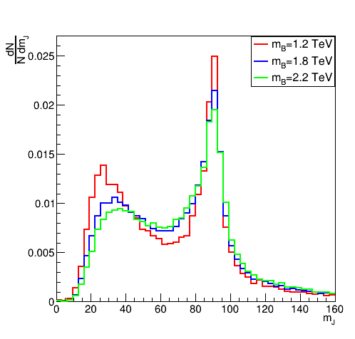
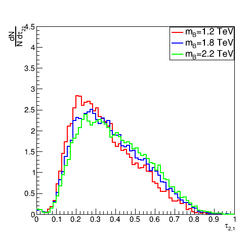
Figure 1:

(left) Mass distribution($m_{j}$) for $Z$-fatjet. (right)$\tau_{21}$ distribution of the $Z$-fatjet. Plots are taken from the study in Ref: [40].

Energy correlation variables: $C_{2}^{\beta}$, $D_{2}^{\beta}$, $N_{2}^{\beta}$

This a a more advanced variable in a sense that unlike N-subjettiness, there is no different minimisation procedure in the algorithm, in order to get the direction of the subjets. More over, energy correlation variables [45] are insensitive to the recoil due to soft emissions. Soft wide angle radiation displaces the hard jet core from the jet axis to balance the angular momentum. N-subjettiness variable is sensitive to this displacement since they are measured with respect to the jet center.

As the $(N+1)$ point correlation functions are sensitive when the jet substructure is $N$-prong, the energy correlation variable is defined as $C_{N}^{\beta}$. As we saw in the ratio of subjettiness, we use $C_{1}^{\beta}$ for QCD jets, $C_{2}^{\beta}$ for bosonic jets, $C_{3}^{\beta}$ for top quark. Here $\beta$ is the angular exponent. The corresponding energy co relation variables are,

$$E^{\beta}_{2}=\sum_{i<j}p_{T_{i}}p_{T_{j}}R_{ij}^{\beta}~{}~{}~{}E^{\beta}_{3}=\sum_{i<j<k}p_{T_{i}}p_{T_{j}}p_{T_{k}}(R_{ij}R_{ik}R_{jk})^{\beta}$$ (19)

$$E^{\beta}_{z}=\sum_{i<j<....<z}p_{T_{i}}p_{T_{j}}...p_{T_{z}}(R_{ij}R_{ik}....\text{all possible combinations})^{\beta}$$ (20)

Just as we saw in case of N-subjettiness ratio, here also ratio of these variables are important. These are defined as,

$$r_{N}^{\beta}=\frac{E(N+1)}{E(N)}~{}~{}~{}~{}~{}~{}~{}C_{N}^{\beta}=\frac{r_{N}^{\beta}}{r_{N-1}^{\beta}}$$ (21)

$C_{N}$ effectively measures higher-order radiation from leading order (LO) substructure. For a system with $N$ subjets, the LO substructure consists of N hard prongs, so if $C_{N}$ is small, then the higher-order radiation must be soft or collinear with respect to the LO structure. If $C_{N}$ is large, then the higher-order radiation is not strongly-ordered with respect to the LO structure, so the system has more than $N$ subjets. Thus, if $C_{N}$ is small and $C_{N}^{1}$ is large, then we can say that a system has $N$ subjets.

5 Conclusion

In this review, I have tried to briefly summarise the main lessons of jet substructure. In the past few years, there have been many theoretical developments in this subject. Moreover, it has seen a huge success at LHC experiments to help to increase the sensitivity of new physics. As the energy of LHC is planned to increased in future, the jet substructure methods will be of huge importance in recent future to study the boosted objects specifically. Advanced techniques such as Neural Network and Machine Learning are opening new doors to study the new physics by making jet substructure more robust. Moreover, there will be implementation of jet substructure in future collider experiments as well. Hence, I believe this era is the golden era for jet substructure in High Energy Physics and this short review might help the beginners to get a basic idea on jet substructure.

References

- [1] S. Marzani, G. Soyez and M. Spannowsky, Looking inside jets: an introduction to jet substructure and boosted-object phenomenology, vol. 958. Springer, 2019, 10.1007/978-3-030-15709-8.
- [2] A. Abdesselam et al., Boosted Objects: A Probe of Beyond the Standard Model Physics, Eur. Phys. J. C 71 (2011) 1661, [1012.5412].
- [3] A. Altheimer et al., Jet Substructure at the Tevatron and LHC: New results, new tools, new benchmarks, J. Phys. G 39 (2012) 063001, [1201.0008].
- [4] D. Adams et al., Towards an Understanding of the Correlations in Jet Substructure, Eur. Phys. J. C 75 (2015) 409, [1504.00679].
- [5] M. Gell-Mann, A Schematic Model of Baryons and Mesons, Phys. Lett. 8 (1964) 214–215.
- [6] G. Sterman, J. Smith, J. C. Collins, J. Whitmore, R. Brock, J. Huston et al., Handbook of perturbative qcd, Rev. Mod. Phys. 67 (Jan, 1995) 157–248.
- [7] R. P. Feynman, Very high-energy collisions of hadrons, Phys. Rev. Lett. 23 (1969) 1415–1417.
- [8] J. D. Bjorken and E. A. Paschos, Inelastic Electron Proton and gamma Proton Scattering, and the Structure of the Nucleon, Phys. Rev. 185 (1969) 1975–1982.
- [9] D. J. Gross, The discovery of asymptotic freedom and the emergence of QCD, Proc. Nat. Acad. Sci. 102 (2005) 9099–9108.
- [10] F. Wilczek, Asymptotic freedom: From paradox to paradigm, Proc. Nat. Acad. Sci. 102 (2005) 8403–8413, [hep-ph/0502113].
- [11] R. K. Ellis, W. J. Stirling and B. R. Webber, QCD and Collider Physics. Cambridge Monographs on Particle Physics, Nuclear Physics and Cosmology. Cambridge University Press, 1996, 10.1017/CBO9780511628788.
- [12] J. C. Collins, Renormalization: An Introduction to Renormalization, the Renormalization Group and the Operator-Product Expansion. Cambridge Monographs on Mathematical Physics. Cambridge University Press, 1984, 10.1017/CBO9780511622656.
- [13] M. Czakon, The Four-loop QCD beta-function and anomalous dimensions, Nucl. Phys. B 710 (2005) 485–498, [hep-ph/0411261].
- [14] D. J. Gross, Nobel lecture: The discovery of asymptotic freedom and the emergence of qcd, Rev. Mod. Phys. 77 (Sep, 2005) 837–849.
- [15] J. J. Ethier and E. R. Nocera, Parton Distributions in Nucleons and Nuclei, Ann. Rev. Nucl. Part. Sci. 70 (2020) 43–76, [2001.07722].
- [16] J. Rojo et al., The PDF4LHC report on PDFs and LHC data: Results from Run I and preparation for Run II, J. Phys. G 42 (2015) 103103, [1507.00556].
- [17] A. D. Martin, Proton structure, Partons, QCD, DGLAP and beyond, Acta Phys. Polon. B 39 (2008) 2025–2062, [0802.0161].
- [18] C. N. Lovett-Turner and C. J. Maxwell, Renormalon singularities of the QCD vacuum polarization function to leading order in 1/N(f), Nucl. Phys. B 432 (1994) 147–162, [hep-ph/9407268].
- [19] G. Sterman and S. Weinberg, Jets from quantum chromodynamics, Phys. Rev. Lett. 39 (Dec, 1977) 1436–1439.
- [20] F. Bloch and A. Nordsieck, Note on the Radiation Field of the electron, Phys. Rev. 52 (1937) 54–59.
- [21] N. N. K. Borah, D. K. Choudhury and P. K. Sahariah, Non-singlet spin structure function g-1(NS) (x,t) in the DGLAP approach, Pramana 79 (2012) 833–837.
- [22] S. Frixione and B. R. Webber, Matching NLO QCD computations and parton shower simulations, JHEP 06 (2002) 029, [hep-ph/0204244].
- [23] S. Frixione, P. Nason and C. Oleari, Matching NLO QCD computations with Parton Shower simulations: the POWHEG method, JHEP 11 (2007) 070, [0709.2092].
- [24] D. Krohn, J. Thaler and L.-T. Wang, Jet Trimming, JHEP 02 (2010) 084, [0912.1342].
- [25] S. D. Ellis, C. K. Vermilion and J. R. Walsh, Recombination Algorithms and Jet Substructure: Pruning as a Tool for Heavy Particle Searches, Phys. Rev. D 81 (2010) 094023, [0912.0033].
- [26] A. J. Larkoski, S. Marzani, G. Soyez and J. Thaler, Soft Drop, JHEP 05 (2014) 146, [1402.2657].
- [27] M. Cacciari, G. P. Salam and G. Soyez, The anti- jet clustering algorithm, JHEP 04 (2008) 063, [0802.1189].
- [28] D. E. Soper, Parton distribution functions, Nucl. Phys. B Proc. Suppl. 53 (1997) 69–80, [hep-lat/9609018].
- [29] A. J. Larkoski, S. Marzani and J. Thaler, Sudakov Safety in Perturbative QCD, Phys. Rev. D 91 (2015) 111501, [1502.01719].
- [30] M. Dasgupta, A. Fregoso, S. Marzani and G. P. Salam, Towards an understanding of jet substructure, JHEP 09 (2013) 029, [1307.0007].
- [31] G. P. Salam, Towards Jetography, Eur. Phys. J. C 67 (2010) 637–686, [0906.1833].
- [32] S. D. Ellis and D. E. Soper, Successive combination jet algorithm for hadron collisions, Phys. Rev. D 48 (1993) 3160–3166, [hep-ph/9305266].
- [33] Y. L. Dokshitzer, G. D. Leder, S. Moretti and B. R. Webber, Better jet clustering algorithms, JHEP 08 (1997) 001, [hep-ph/9707323].
- [34] G. C. Blazey et al., Run II jet physics, in Physics at Run II: QCD and Weak Boson Physics Workshop: Final General Meeting, pp. 47–77, 5, 2000. hep-ex/0005012.
- [35] J. Gallicchio and M. D. Schwartz, Quark and Gluon Tagging at the LHC, Phys. Rev. Lett. 107 (2011) 172001, [1106.3076].
- [36] S. D. Ellis, C. K. Vermilion and J. R. Walsh, Techniques for improved heavy particle searches with jet substructure, Phys. Rev. D 80 (2009) 051501, [0903.5081].
- [37] CMS collaboration, A Cambridge-Aachen (C-A) based Jet Algorithm for boosted top-jet tagging, .
- [38] T. Plehn, M. Spannowsky, M. Takeuchi and D. Zerwas, Stop Reconstruction with Tagged Tops, JHEP 10 (2010) 078, [1006.2833].
- [39] J. Shelton, Jet Substructure, in Theoretical Advanced Study Institute in Elementary Particle Physics: Searching for New Physics at Small and Large Scales, pp. 303–340, 2013. 1302.0260. DOI.
- [40] D. Choudhury, K. Deka and N. Kumar, Looking for a vectorlike B quark at the LHC using jet substructure, Phys. Rev. D 104 (2021) 035004, [2103.10655].
- [41] R. Kogler et al., Jet Substructure at the Large Hadron Collider: Experimental Review, Rev. Mod. Phys. 91 (2019) 045003, [1803.06991].
- [42] CMS collaboration, A. Sirunyan et al., Search for pair production of vector-like T and B quarks in single-lepton final states using boosted jet substructure in proton-proton collisions at TeV, JHEP 11 (2017) 085, [1706.03408].
- [43] CMS collaboration, A. M. Sirunyan et al., Search for electroweak production of a vector-like quark decaying to a top quark and a Higgs boson using boosted topologies in fully hadronic final states, JHEP 04 (2017) 136, [1612.05336].
- [44] J. Thaler and K. Van Tilburg, Identifying Boosted Objects with N-subjettiness, JHEP 03 (2011) 015, [1011.2268].
- [45] A. J. Larkoski, G. P. Salam and J. Thaler, Energy Correlation Functions for Jet Substructure, JHEP 06 (2013) 108, [1305.0007].