LibSignal: An Open Library for Traffic Signal Control

Abstract

This paper introduces a library for cross-simulator comparison of reinforcement learning models in traffic signal control tasks. This library is developed to implement recent state-of-the-art reinforcement learning models with extensible interfaces and unified cross-simulator evaluation metrics. It supports commonly-used simulators in traffic signal control tasks, including Simulation of Urban MObility(SUMO) and CityFlow, and multiple benchmark datasets for fair comparisons. We conducted experiments to validate our implementation of the models and to calibrate the simulators so that the experiments from one simulator could be referential to the other. Based on the validated models and calibrated environments, this paper compares and reports the performance of current state-of-the-art RL algorithms across different datasets and simulators. This is the first time that these methods have been compared fairly under the same datasets with different simulators.

1 Introduction

Traffic signals coordinate the traffic movements at the intersection, and a smart traffic signal control algorithm is the key to transportation efficiency. Traffic signal control remains an active research topic because of the high complexity of the problem. The traffic situations are highly dynamic and thus require traffic signal plans to adjust to different situations. People have recently started investigating reinforcement learning (RL) techniques for traffic signal control. Several studies have shown the superior performance of RL techniques over traditional transportation approaches wei2018intellilight ; wei2019presslight ; xu2021hierarchically ; oroojlooy2020attendlight ; ma2020feudal . The biggest advantage of RL is that it directly learns how to take the next actions by observing the feedback from the environment after previous actions.

In literature, a number of traffic signal control methods have been proposed yau2017survey ; wei2019survey , and it has attracted much attention to facilitate the implementation or use of these proposed methods. However, as shown in Table 1, current methods are distributed among different simulators and datasets. As we will show later in this paper, datasets, simulators, and even evaluation metrics vary the performance for the same algorithm. In addition, reinforcement learning is also sensitive to hyper-parameters. All these make it difficult for new traffic signal control methods to ensure effective and uniform improvement. Therefore, there is an urgent need for a cross-platform, unified process with extensible code base that supports multiple models.

This paper presents a unified, flexible, and comprehensive traffic signal control library named LibSignal. Our library is implemented based on PyTorch and includes all the necessary steps or components related to traffic signal control into a systematic pipeline. We consider two mainstream simulators, SUMO and CityFlow, and provide various datasets, models, and utilities to support data preparation, environment calibration, model instantiation, and performance evaluation for the two kinds of simulators.

Contributions: To the best of our knowledge, LibSignal is the first open-source library that provides benchmarking results for traffic signal control methods across various datasets and simulators.The main features of LibSignal can be summarized in three aspects:

• Unified: LibSignal builds a systematic pipeline to implement, use and evaluate traffic signal control models in a unified platform. We design cross-simulator data configuration, unified model instantiation interfaces, and standardized evaluation procedures.

• Comprehensive: 10 models covering two traffic simulators have been reproduced to form a comprehensive model warehouse. Meanwhile, LibSignal collects 9 commonly used datasets from different sources, makes them compatible for both simulators, and implements a series of commonly used evaluation metrics and strategies for performance evaluation.

• Extensible: LibSignal enables a modular design of different components, allowing users to flexibly insert customized components into the library. It also has an OpenAI Gym interface gym2016 which allows easy deployment of standard RL algorithms.

What LibSignal isn’t: Despite the ability to train and test across different simulators, LibSignal does not claim the performances of the same model on different simulators are identical. There are some differences of internal mechanisms between different simulators, for example, vehicle’s maneuver behaviors, and our emphasis is on the relative performance of compatible policies we provide. This makes LibSignal a possible testbed for Sim-to-Real transfer zhao2020sim ; peng2018sim , which is not covered by this paper.

Table 1: Summary of the state-of-the-art models (a partial list), sorted by citations from Google Scholar by 2022/06/08. Full list can be found in https://darl-libsignal.github.io/.

Method	Venue	Cite	Simulator	Dataset (* means open accessed)	Main Metrics
IntelliLight wei2018intellilight	KDD 2018	321	SUMO	Jinan 1x1	Travel Time, speed, queue length, approximated delay
IDQN  https://doi.org/10.48550/arxiv.1905.04716	arXiv 2019	53	SUMO	LA 1x4*, Jinan 1x1, Hangzhou 1x1	Travel Time
MAPG chu2019multi	TITS 2019	308	SUMO	Grid 4x4, Monaco*	Approximated delay, queue length
CoLight wei2019colight	CIKM 2019	116	CityFlow	Hangzhou 4x4*, Jinan 3x4*, Manhattan 3x27*	Travel Time
MPLight chen2020toward	AAAI 2020	98	CityFlow	Grid 4x4, Manhattan	Travel time, throughput
PressLight wei2019presslight	KDD 2019	93	CityFlow	Jinan 1x3, State College*, Mahattan*	Travel time
FRAP zheng2019learning	CIKM 2019	67	CityFlow	Hangzhou 1x1*, Atlanta 1x5*	Travel Time
MetaLight zang2020metalight	AAAI 2020	43	CityFlow	Hangzhou 1x1*, Atlanta 1x5*, Hangzhou 4x4*, Jinan 3x4*	Travel time
DemoLight xiong2019learning	CIKM 2019	22	CityFlow	Hangzhou 1x1*	Travel Time
FMA2C  ma2020feudal	AAMAS 2020	16	SUMO	4x4 Grid, Monaco*	Queue length, throughput, delay
TPG  rizzo2019time	KDD 2019	15	SUMO	Roundabout	Queue length, waiting time, throughput, speed
AttendLight oroojlooy2020attendlight	NeurIPS 2020	12	CityFlow	Hangzhou 4x4*, Atlanta 1x5*	Travel time
HiLight xu2021hierarchically	AAAI 2021	12	CityFlow	Hangzhou 4x4*, Jinan 3x4*, Manhattan 3x27*, Shenzhen*	Travel time, throughput
IG-RL devailly2021ig	TITS 2021	11	SUMO	Manhattan	Approximated delay
ExplainPG rizzo2019reinforcement	ITSC 2019	11	SUMO	Roundabout	Waiting time, throughput
RACS-R wang2021traffic	TITS 2021	6	SUMO	Monaco*	Waiting time, queue length
GeneraLight zhang2020generalight	CIKM 2020	4	CityFlow	Hangzhou 1x1*, Atlanta 1x5*, Hangzhou 4x4*	Travel time
OP-TSC yen2020deep	ITSC 2020	4	SUMO	synthetic	Delay
DFC raeis2021deep	ITSC 2021	2	SUMO	synthetic	Waiting time
DynSTGAT wu2021dynstgat	CIKM 2021	0	CityFlow	Hangzhou 4x4*, Jinan 3x4*, Grid 4x4*	Travel time, throughput
EMV cao2022gain	TITS 2022	0	SUMO	Hangzhou 4x4*	Waiting time, queue length

2 Background

2.1 Reinforcement Learning for Traffic Signal Control

Problem formulation

We now introduce the general setting of the RL-based traffic signal control problem, in which the traffic signals are controlled by an RL agent or several RL agents. The environment is the traffic conditions on the roads, and the agents control the traffic signals’ phases. At each time step $t$, a description of the environment (e.g., signal phase, waiting time of cars, queue length of cars, and positions of cars) will be generated as the state $\mathsf{s}^{t}$. The agents will predict the next actions $\mathsf{a}^{t}$ to take that maximize the expected return, where the action of a single intersection could be changing to a certain phase. The actions $\mathsf{a}^{t}$ will be executed in the environment, and a reward $\mathsf{r}^{t}$ will be generated, where the reward could be defined on the traffic conditions of the intersections.

Basic components of RL-based traffic signal control

A key question for RL is how to formulate the RL setting, i.e., the reward, state and action definition. For more discussions on the reward, state, and actions, we refer interested readers to yau2017survey ; rasheed2020deep ; wei2021recent . There are three main components to formulate the problem under the framework of RL:

• Reward design. As RL is learning to maximize a numerical reward, the choice of reward determines the direction of learning. A typical reward definition for traffic signal control is one factor or a weighted linear combination of several components such as queue length, waiting time and delay.

• State design. State captures the situation on the road and converts it to values. Thus the choice of states should sufficiently describe the environment. The state features queue length, the number of cars, waiting time, and the current traffic signal phase. Images of vehicles’ positions on the roads can also be considered into the state.

• Selection of action scheme. Different action schemes also have influences on the performance of traffic signal control strategies. For example, if the action of an agent is acyclic, i.e., “which phase to change to”, the traffic signal will be more flexible than a cyclic action, i.e., “keep current phase or change to the next phase in a cycle”.

2.2 Difficulties in Evaluation

In practice, the evaluation of traffic signal control methods could be largely influenced by simulation settings, including the evaluation metrics and simulation environments.

Evaluation metrics

Various measures have been proposed to quantify the efficiency of the intersection from different perspectives, including the average delay of vehicles, the average queue length in the road network, the average travel time of all vehicles, and the throughput of the road network. Signal induced delay is another widely used metric, and previous work suggested real-time approximation as the difference between the vehicle’s current speed and the maximum speed limit over all vehicles. But as we will show in Section 4.2, this approximated delay is not reflecting the actual delay. Queue length is another mostly used metrics wei2018intellilight , while different definitions of a "queuing" state of a vehicle could largely influence the performance of the same method. In comparison, travel time and throughput are more robust to ad-hoc definitions and approximations. As we will show later, with the same experimental setting, the performance of the same method could be different under different metric, and we aim to provide as comprehensive and flexible metrics as possible in this paper to benchmark methods with a comprehensive view.

Simulation environments

Since deploying and testing traffic signal control strategies in the real world involve high cost and intensive labor, simulation is a useful alternative before actual implementation. Different choices of simulator could lead to different evaluation performances.

Currently, there are two representative open-source microscopic simulators: Simulation of Urban MObility (SUMO) sumo2018 and CityFlow zhang2019cityflow . SUMO is widely accepted in the transportation community and is a reasonable testbed choice. Compared with SUMO, CityFlow is a simulator optimized for reinforcement learning with faster simulation, while it is not widely used by the transportation field yet.

Because of these different simulation environments, methods adopted by different simulators in their original papers are hard to evaluate. As we will show later, methods perform differently under different well-calibrated simulators, and the efficiency of the training process is also different under different simulators. This paper, for the first time, compares the performances of the same model under the same traffic datasets under different simulators.

2.3 Existing Libraries and Tools

websiteTSC is an open-source library that provides a bunch of RL-based traffic signal control methods with traffic datasets only on CityFlow zhang2019cityflow . Flow kheterpal2018flow and RESCO ault2021reinforcement are reinforcement learning frameworks that can support the design and experimentation of traffic signal control methods only on SUMO sumo2018 . TSLib tslib2021 is another library that could work under both SUMO and CityFlow, yet it has limited extensibility: (1) it is difficult to deploy standard RL algorithms since it does not have an OpenAI Gym interface; (2) there are no benchmarking datasets that work across both simulators, which makes it challenging to help determine which algorithm results in state-of-the-art performance.

3 LibSignal Toolkit

We propose LibSignal library integrating different influential traffic flow simulators and denote it as a standard RL traffic control testbed. The primary purposes of this standard testbed are:

• Provide a converter to transform configurations including road networks and traffic flow files across different simulators, enabling comparisons between different algorithms originally conducted in different simulators.

• A standardized implementation of state-of-the-art RL-based and traditional traffic control algorithms.

• A cross-simulator environment provides highly unified functions to interact with different baselines or user-defined models and supports performance comparisons among them.

LibSignal is open source and free to use/modify under the GNU General Public License 3. The code is built on top of GeneraLight zhang2020generalight and is available on Github at  https://darl-libsignal.github.io/. The embedded traffic datasets are distributed with their own licenses from websiteTSC and ault2021reinforcement , whose licenses are under the GNU General Public License 3. SUMO is licensed under the EPL 2.0, and CityFlow is under Apache 2.0. The overall framework of LibSignal is presented in Figure 1, and the implementation details will be introduced in the following sections.

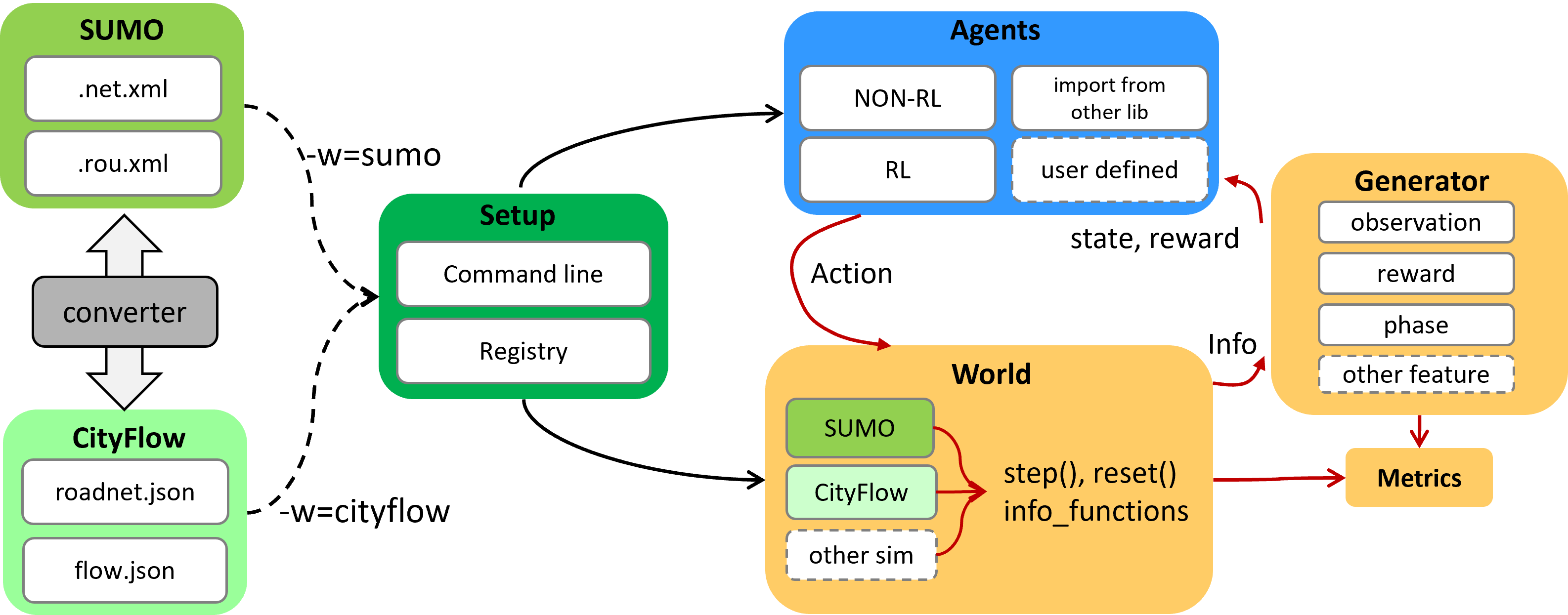
Figure 1: Overall framework of LibSignal

3.1 Data Preparation

To enable fair comparison, LibSignal preprocesses comprehensive datasets making it runnable under different simulators. Users can easily choose to specify datasets and simulators for their experiments.

Comprehensive datasets

By surveying the recent literatures on traffic prediction, we selected 225 representative or survey papers (more details can be found in Table 1). We collected all the open datasets used by these papers and kept 9 datasets according to the factors of popularity, which can cover 65% papers of our reproduced model list and all the two simulators LibSignal supports. To directly use these datasets in LibSignal, we have converted all the 9 datasets into the format of atomic files, and provided the conversion tools for new datasets. Please refer to our GitHub page for dataset statistics, preprocessed copies, and conversion tools at  https://darl-libsignal.github.io/.

Cross-simulator atomic files

To make the experimental configuration adaptive across different simulators, we consider two basic units called “atomic files" that can map to the different simulation environments. 1) Road network file stores the basic structure of a traffic network consisting of road, lane, and traffic light information. The atomic file under the SUMO environment is in the format of .net.xml while in CityFlow it’s .json. 2) Traffic flow file stores the vehicles information and is in .rou.xml and .json format in SUMO and CityFlow respectively. To make experiments comparable among different simulators, we also provide a converter.py tool to convert basic atomic files between different simulators. For example, it takes in Road network file and Traffic flow file from the source simulator and generates new files in the target simulator’s formation, which could later be used in experiments. Figure 3 shows the converted network between different simulators.

3.2 Traffic Signal Control Environment

Once the necessary parameters have been set up for simulation and agents, we can start a traffic light control task experiment. The World environment is highly homogeneous across different simulators and could provide unified interfaces to communicate with different agents.

Homogeneous world

In LibSignal, World module provides the basic information from different simulators in unified interfaces compatible with OpenAI Gym gym2016 , which could later be utilized for interacting between different simulators and Agent. In the World class, we provide an info_functions object inside to help retrieve information from different simulator environments and update information after each simulator performs a step. The info_functions contain state information including lane_count, lane_waiting_count, lane_waiting_time count, pressure, phase ,and metrics including throughput, average_travel_time, lane_delay, lane_vehicles. These info_functions will later be called by Generator class and pass information into Agent. step() function is another common function shared between different World classes. It takes in actions returned from Agent class and passes them into the simulator for next step execution. And action is either sampled from action space for exploration or calculated from the model after optimization. Generally, the action space contains eight phases. However, in highly heterogenous traffic structures, the action space may differ and is provided by the simulators whose action parameters are taken from configuration files.

Unified interfaces

LibSignal provides unified interfaces to process common information with Generator module and Metrics module. For lane level information, including state, reward, phase, and other lane level metrics, we provide Generator module, which could interact with different World classes and then sort and pass information to different Agent classes. The state, reward, and phase information will later be utilized by Agent module to train their models or decide next step actions and feedback to World module. At the same time, the other lane level metrics, including queue length and lane delay, will be passed to Metrics module for model evaluation. LibSignal currently supports four metrics: the average delay of vehicles (delay), the average queue length in the road network (queue), the average travel time of all vehicles (travel time), and the throughput of the road network (throughput). Their detailed calculation can be found in Appendix.

3.3 Comprehensive Models

LibSignal implements three baseline controllers and seven RL-based controllers covering Q-learning and Actor-Critic methods, as is shown in Table 2. These methods can also be integrated with existing RL implementation packages and customized on their state, action, and reward design.

Table 2: Detailed design of implemented models in LibSignal.

Agent	State	Action	Reward	Method	Description
FixedTime	-	Cyclic	-	Non-RL	This agent gives a predefined time duration and phase order.
SOTL	-	Acyclic	-	Non-RL	This agent selects the phase among all to maximize the pressure calculated from the upstream and downstream queue length.
MaxPressure	-	Acylic	-	Non-RL	This agent determines next phase by considering competitive phases.
IDQN	lane vehicle count, phase	Acylic	lane waiting vehicle count	Q-Learning	This agent determines each intersection’s action with its own intersection information.
CoLight	lane vehicle count, phase	Acylic	lane waiting vehicle count	Q-Learning	This agent considers neighbor intersections’ cooperation through graph attention networks.
PressLight	lane vehicle count, phase	Acylic	pressure	Q-Learning	This agent coordinates traffic signals by learning MaxPressure.
IPPO	lane vehicle count, phase	Acylic	lane vehicle waiting time count	Actor-Critic	This agent is imported from pfrl with proximal policy optimization.
MAPG	lane vehicle count	Acylic	lane waiting vehicle count	Actor-Critic	This agent optimizes agent control policy with muti-agent policy gradient method.
FRAP	lane vehicle count, phase	Acylic	lane waiting vehicle count	Q-Learning	This agent captures the phase competition relation between traffic movements through a modified network structure.
MPLight	pressure, phase	Acylic	pressure	Q-Learning	This agent is based on FRAP and integrates pressure into state and reward design.

Extensible design

LibSignal provides a flexible interface to help users customize their own RL model and RL design (state, reward, and action). Users can define their model through Agent module by completing abstract methods predefined in BaseAgent class. Existing RL libraries like pfrl can also be integrated into Agent class. LibSignal also provide different state and reward functions by instantiating Generator with subscribed function names in info_functions to retrieve queue length, pressure, average lane speed, etc. Users could also customize their own reward or state functions by constructing a key-value mapping between new defined functions and info_functions, which could be carried to Agent later by Generator class.

4 Experiment

In this section, we first present our result and verify that our implementation is consistent with previous publications. In the second part, we compare different algorithms’ performance with different datasets in both SUMO and CityFlow. Finally, we test the feasibility of LibSignal to verify it can properly run on large-scale and complex road net. Further, we also adapt algorithms from widely used RL library to testify our Agent module is flexible and easy to manipulate. Along the experiments, we will discuss the answers to several questions that motivate LibSignal: Which simulator should I conduct experiments on? Which evaluation metrics should I use? Which RL method should I choose? Is LibSignal suitable for my research?

4.1 Validation and Calibration

For testifying our PyTorch benchmark algorithms implementation, we compare the learning curves and final performances of the RL algorithms originally implemented in TensorFlow library. The simulator setting and observed traffic information are chosen to be similar to those used in previous publications.

TensorFlow to PyTorch validation To validate the model’s performance under the framework, LibSignal re-implemented some of the previous models from Tensorflow with PyTorch. For example, IDQN https://doi.org/10.48550/arxiv.1905.04716 and CoLight wei2019colight are originally implemented in Tensorflow, we reproduce the experiments of these models and compare their performance in CityFlow simulator. Figure 2 presents the learning curves and final performance of the original TensorFlow and our PyTorch implementation. On CityFlow1x1, the average travel time (in seconds) of our IDQN implementation converges to 116.28 which is also close to the original’s 127.07 from https://doi.org/10.48550/arxiv.1905.04716 . Our CoLight implementation converges to 344.41 on average travel time metric, which is close to TensorFlow’s 344.49 from wei2019colight .

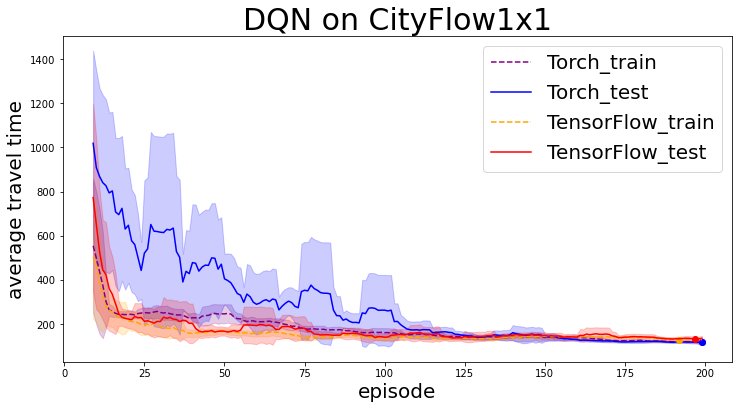
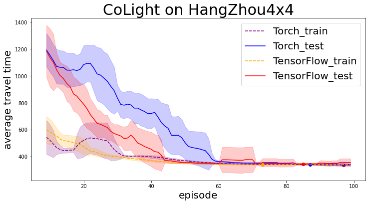
(a) IDQN in CityFlow1x1	(b) CoLight in HangZhou4x4

Figure 2: Convergence curve of models implemented in their original form (Tensorflow) and in LibSignal (PyTorch). Y-axis are the testing results w.r.t. average travel time (in seconds). Validation for more models can be found in Appendix.

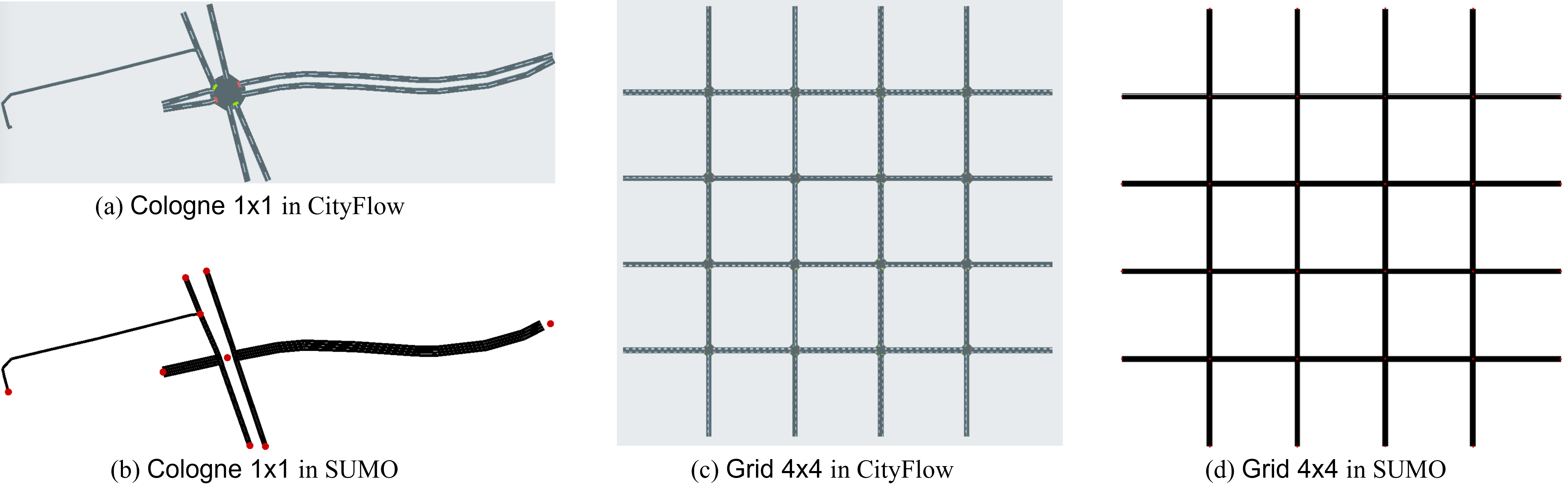
Figure 3: Road networks in different simulators for calibration The pictures with a gray background are the visualization of networks in the SUMO simulator, and the ones with the white background are in CityFlow. These are the outlines of traffic structures transferred between each other(More networks can be found in Appendix).

SUMO and CityFlow calibration. To validate the algorithms performances are consistent in both SUMO and CityFlow, we calibrate under three road networks Grid4x4, Cologne1x1 and HangZhou4x4. Their road network is shown in Figure 3. In addition, we compare MaxPressure, SOTL and FixedTime algorithms performance since these three algorithms are deterministic given fixed network and traffic flow files. Table 3 shows the overall performance before and after calibration. We have the following observations:

Table 3: Performance comparison of agents w.r.t. average travel time (in seconds) before and after calibration

Calibration	Before						After
Dataset	Grid4x4		Cologne1x1		HangZhou4x4		Grid4x4		Cologne1x1		HangZhou4x4
Avg. Travel Time	Cityflow	SUMO	Cityflow	SUMO	Cityflow	SUMO	Cityflow	SUMO	Cityflow	SUMO	Cityflow	SUMO
MaxPressure	161.2878	143.8296	51.2785	56.9068	365.0634	255.0052	142.5275	143.8296	58.3441	56.9068	365.0634	350.4125
FixedTime	290.9525	194.6542	156.6599	257.4194	689.0221	300.6685	179.6606	194.6542	206.4620	257.4194	689.0221	535.0060
SOTL	185.8846	208.3936	1356.6037	49.9770	354.1250	389.7881	187.8568	208.3936	50.5813	49.9770	354.1250	386.7881

$\bullet$ Under gird-like networks (Grid4x4, HangZhou4x4), SUMO and CityFlow could achieve similar performance. Different agents’ performance is not identical across simulators, but their rank within the same simulator is relatively consistent.  
 $\bullet$ The discrepancy appears under more complex networks like Cologne1x1 before calibration. Before calibration, we can see that FixedTime and SOTL perform worse than MaxPressure. After calibration, the same agent’s performance is close and within an acceptable discrepancy between SUMO and CityFlow. Moreover, the ranking of the performances for different agents is consistent across different simulators after calibration. To double check our calibration is correct, IDQN algorithms are also trained under Cologne1x1 with different simulators. In CityFlow and SUMO simulator, the results are 50.581 and 49.977 in Cologne1x1 w.r.t average travel time (in seconds), which further proved our calibration is correct.

We modified some default settings in SUMO to compare the algorithms’ performance under different simulators as comprehensively and fairly as possible, e.g., disabled the feature of dynamic routing and set teleport to be -1. But it is worth noting that there are still some discrepancies that our current calibration cannot address. For example, SUMO has pedestrian traffic signals that CityFlow does not support, where vehicles will decelerate when they encounter the pedestrian traffic signals in SUMO and in CityFlow the vehicles will pass the intersection at normal speed. In addition, the vehicles in SUMO will also randomly decelerate when approaching a traffic signal even though the traffic signal is located further away; In comparison, the vehicles in CityFlow will not have such randomness.

4.2 Overall Performance

For comparative purposes, all benchmark RL models and traditional traffic control algorithms were compared under different simulator environments. All observations and rewards are set to be the same if not specifically mentioned, and all the hyperparameters are set according to the original implementations. We represent the final results truncated at 200 training iterations for a fair comparison, since most algorithms could converge within this period. While IPPO and MAPG are noticeable for their high demand for training time, we provide the full converge curve in the Appendix. The results are summarized in Table 4. We have the following observations:  
 $\bullet$ Under the same dataset and simulator, the performance of the same model varies w.r.t. current four metrics. Travel time and queue length are consistent with each other in most cases. Throughput sometimes is hard to differentiate the identical results under certain datasets. For example, in Grid4x4, all the methods served the same number of vehicles. Delay sometime aligns with queue length and travel time, but can be different from all the other three metrics in some cases, e.g., Cologne1x3 under CityFlow and Grid4x4 under SUMO. This is because the delay is approximated from the average speed proposed by ault2021reinforcement and is not the actual delay calculated by vehicles’ total travel time and desired travel time under maximum speed.  
 $\bullet$ Traditional transportation methods like MaxPressure can achieve consistent satisfactory performance though it is not the best. IDQN performs the best in single intersection scenarios. With more complicated road networks like Cologne1x1 and Cologne1x3, PressLight achieves better performance.

Table 4: Performance of agents in CityFlow and SUMO with best and second best performance highlighted.

Network	Cityflow 1x1
Simulator	CityFlow				SUMO
Metric	Travel Time	Queue	Delay	Throughput	Travel Time	Queue	Delay	Throughput
FixedTime(t_fixed=10)	923.6665	114.4167	4.8309	1006	533.0330	91.9500	4.3162	848
FixedTime(t_fixed=30)	552.7249	100.3444	5.1862	1455	270.6999	80.4389	5.6198	1546
MaxPressure	303.8070	100.9444	6.7686	1717	137.9254	43.3417	6.2455	1930
SOTL	212.2152	69.1056	5.4247	1861	154.7708	50.5583	5.1124	1915
IDQN	116.6373	28.3706	0.6111	1959	91.7185	16.4861	0.5397	1968
MAPG	490.7145	118.6139	0.7392	1514	235.1756	108.7583	0.7089	655
IPPO	308.8728	95.3806	0.7578	1736	182.7708	79.1167	0.7103	1492
PressLight	105.6764	23.2028	0.5754	1965	97.5526	20.0306	0.5523	1969
FRAP	104.2751	23.2944	0.6225	1979	89.9246	14.9000	0.5426	1963
Network	Cologne 1x1
Simulator	CityFlow				SUMO
Metric	Travel Time	Queue	Delay	Throughput	Travel Time	Queue	Delay	Throughput
FixedTime(t_fixed=10)	206.4620	51.5889	4.0432	1847	257.4194	86.1139	6.2857	1471
FixedTime(t_fixed=30)	156.9632	46.2278	4.2243	1910	109.2111	40.2056	5.4129	1947
MaxPressure	58.3441	7.6944	2.7739	2002	56.9068	10.4306	3.4879	1996
SOTL	1358.6191	104.6083	5.9367	515	277.9961	97.7722	7.1510	511
IDQN	50.5813	5.3667	0.3117	2000	49.9770	7.1250	0.3828	1999
MAPG	46.7260	5.0639	0.3002	2000	1105.5855	64.7528	0.4953	152
IPPO	55.7449	7.3500	0.3334	1994	1134.2086	64.4167	0.4941	163
PressLight	51.7887	4.8222	0.2940	2001	54.5398	9.4028	0.4199	1997
FRAP	66.6718	12.0889	0.3094	1995	93.4075	29.3444	0.5994	1951
Network	Cologne 1x3
Simulator	CityFlow				SUMO
Metric	Travel Time	Queue	Delay	Throughput	Travel Time	Queue	Delay	Throughput
FixedTime(t_fixed=10)	93.3808	4.8028	1.5649	2791	108.0544	10.0991	2.5904	2793
FixedTime(t_fixed=30)	91.9379	5.9120	1.7413	2781	118.0659	9.9722	3.1455	2794
MaxPressure	56.6100	1.5667	1.1976	2787	59.5518	1.2852	1.3130	2818
SOTL	1413.4136	48.5324	4.1193	735	306.5369	53.8917	5.1416	1058
IDQN	69.5980	2.0667	0.2076	3509	60.1986	1.1225	0.1848	2820
MAPG	67.1616	6.6310	0.1769	1204	1276.6503	49.4509	0.6361	1086
IPPO	57.2221	1.6370	0.2679	2792	70.0917	3.2630	0.2962	2813
PressLight	53.4214	0.8065	0.1284	2790	77.0971	2.9648	0.2139	2822
MPLight	52.9214	1.2926	0.1271	2790	96.1173	3.4630	0.2282	2821
Network	Grid4x4
Simulator	CityFlow				SUMO
Metric	Travel Time	Queue	Delay	Throughput	Travel Time	Queue	Delay	Throughput
FixedTime(t_fixed=10)	179.6606	1.2889	1.2128	1473	194.6542	1.9967	1.2571	1443
FixedTime(t_fixed=30)	258.1894	3.3891	2.0448	1465	292.0315	4.4988	2.2300	1428
MaxPressure	142.8568	0.5010	0.6866	1473	143.8296	0.6276	0.5197	1461
SOTL	187.8568	1.5012	1.2580	1473	208.3936	2.3321	1.3739	1443
IDQN	133.8038	0.2540	0.0411	1473	143.3112	0.5997	0.0402	1462
MAPG	227.6490	2.4816	0.1259	1473	225.4148	2.4328	0.1277	1471
IPPO	197.8900	1.7667	0.1134	1473	206.2505	2.3151	0.1154	1437
PressLight	142.3299	0.4528	0.0542	1473	147.2203	0.6978	0.0456	1462
CoLight	138.6857	0.4038	0.0476	1473	143.9758	0.6288	0.0437	1461
MPLight	140.8452	0.3976	0.0513	1473	158.4627	1.0156	0.0600	1461

We also conducted experiments for different network scalability and complexity, and the results can be found in the Appendix.

4.3 Discussion

Which simulator should I conduct experiments on?

From the running time comparison in Table 5 between SUMO and CityFlow simulator, we find that CityFlow and SUMO (with Libsumo)’s time cost is around ten times less than SUMO (with TraCI) which indicates its higher running efficiency. Different from CityFlow, SUMO provides a more accurate depiction of vehicles’ state and more complex traffic operations, including changing lanes and ’U-turn’. Also, SUMO provides users with more realistic settings, including pedestrians, driver imperfection, collisions, and dynamic routing. Thus, it is more powerful on complex networks and reflecting real-world scenario.

Table 5: Performance comparison w.r.t. the running time (in seconds) of different methods under two simulators.

Running Time	Simulator	FixedTime	MaxPressure	SOTL	IDQN	IPPO	PressLight
Cityflow1x1	CityFlow	5.7593	9.5857	6.0272	2461.7496	2450.7397	1960.7932
	SUMO(Libsumo)	6.0006	4.2174	4.2988	3691.8403	2833.0523	3619.1282
	SUMO(Traci)	73.6791	46.5712	51.488	30279.5201	37662.9677	27697.9098
Cologne1x1	CityFlow	3.3049	2.7601	4.6527	1641.6128	3148.0649	3066.7189
	SUMO(Libsumo)	4.3649	3.1411	3.2771	2649.0341	2581.8182	2863.9526
	SUMO(Traci)	133.6334	24.9327	71.7565	11243.2917	31431.1760	11535.0851

Which evaluation metrics should I use?

Average travel time is generally a good metric to evaluate algorithms’ performance on traffic control tasks. But for settings with dynamic routing, the travel time would not be a good metric as the average travel time of a vehicle can change with dynamic routing. In LibSignal, the simulation under SUMO disabled the feature of dynamic routing so the travel time would be good on the current settings. From Table 4, we can see that lane delay and throughput are not always consistent between different simulators and even in the same simulator environment. Sometimes they often show contradictory performances in different datasets. Therefore, we suggest researcher report travel time as a necessity, and other metrics of their interest in their papers.

Which RL method should I choose?

From our experiments in Table 4, we can see that Actor-Critic based RL algorithms need a long time to converge. In Cologne1x1, MAPG and IPPO algorithms still perform badly after 200 iterations. IDQN and other Q-learning-based algorithms are generally good choices in all five datasets. We can see that they outperform traditional non-RL algorithms all the time. Comparing results in CityFlow1x1 and Cologne1x3, we find FRAP and MPLight could bring improvement compared to IDQN algorithm.

When should I use LibSignal?

Since LibSignal provides a highly unified interface to help users choose or define their functions and extract information from the simulator’s environment, it is a powerful platform for users to investigate the best combination of state and reward functions for current state-of-the-art or their implemented models. Also, users could compare their algorithms with our implemented baseline model using the evaluation metrics we provided. In addition, since LibSignal supports multiple simulation environments, users could also conduct experiments in the different simulation environments to validate that their algorithms are robust and achieve generally good performance under different settings.

When shouldn’t I use LibSignal?

Currently, LibSignal only supports SUMO and CityFlow, thus users currently cannot run their experiments with other simulation engines in our library unless implementing an World like LibSignal did for SUMO and CityFlow. Also, users might need to spend extensive labor to compare their experiment results across simulators if they use their datasets because of dataset calibration. Furthermore, if users plan to use algorithms with extra information like FRAP zheng2019learning , they might need to define competitive phases, and the implementation of their agents under complex or large-scale network which should be rather complicated.

5 Conclusion

In this paper, we introduced LibSignal, a highly unified, extensible, and comprehensive library for traffic light control tasks. We collected and filtered nine commonly used datasets and implemented ten different baseline models across two influential traffic simulators, including SUMO and CityFlow. We both conducted experiments to prove our PyTorch implementation could achieve the same level of performance as the original TensorFlow official code and calibrated simulators to improve the reliability of our cross-simulator environment. Moreover, the performance of all implemented algorithms was compared under various datasets and simulators. We further provided the discussion for researchers interested in this topic with our benchmarking results.In the future, we will implement more state-of-the-art RL-based algorithms and continually support more simulator environments. Further calibration efforts will be made to help different algorithms’ performance comparisons across different simulators.

Appendix A Appendix

A.1 Documentation and License

LibSignal is open source and free to use/modify under the GNU General Public License 3. The code and documents are available on Github at https://darl-libsignal.github.io/. The embedded traffic datasets are distributed with their own licenses from websiteTSC and ault2021reinforcement , whose licenses are under the GNU General Public License 3. SUMO is licensed under the EPL 2.0 and CityFlow is under Apache 2.0. All experiments can be reproduced from the source code, which includes all hyper-parameters and configuration. The authors will bear all responsibility in case of violation of rights, etc., ensure access to the data and provide the necessary maintenance.

A.2 Metrics Definition

Average travel time (travel time): The average time that each vehicle spent on traveling within the network, including waiting time and actual travel time. A smaller travel time means the better performance.

Queue length (queue): The average queue length over time, where the queue length at time $t$ is the sum of the number of vehicles waiting on lanes. A smaller queue length means the better performance.

Approximated delay (delay): Averaged difference between the current speed of vehicle and the maximum speed limit of this lane over all vehicles, calculated from $1-\frac{\sum_{i=1}^{n}v_{i}}{n*v_{max}}$ ault2021reinforcement , where $n$ is the number of vehicles on the lane, $v_{i}$ is the speed of vehicle $i$ and $v_{max}$ is the maximum allowed speed. A smaller delay means the better performance.

Real delay (real delay): Real delay of a vehicle is defined as the time a vehicle has traveled within the environment minus the expected travel time. A smaller delay means better performance.

Throughput: Number of vehicles that have finished their trips until current simulation step. A larger throughput means the better performance.

A.3 Validation

To validate our PyTorch re-implementations performance, we compare the performance of four algorithms which originally implemented in TensorFlow. Fig 4 shows the converge curve of MAPG, PressLight, IDQN, and CoLight in both the train and test phase, which are not provided in Section 4.1. The final performance in Table 6 shows that all four new implementations are consistent with their original TensorFlow implementations.

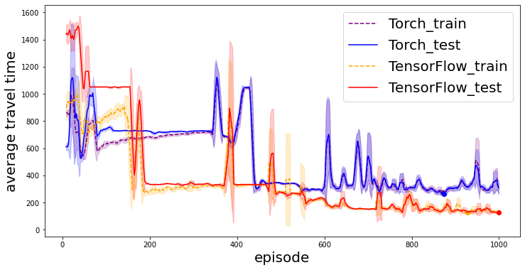
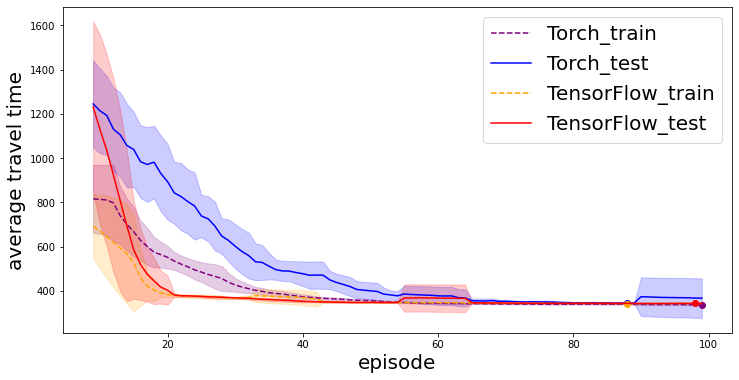
(a) MAPG in CityFlow1x1	(b) PressLight in HangZhou4x4
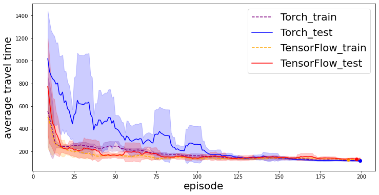
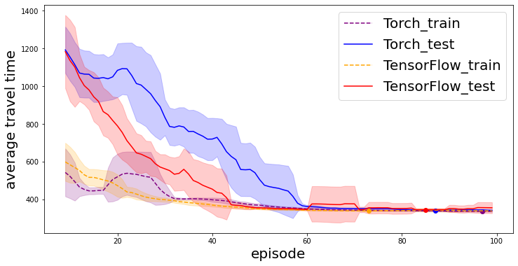
(a) IDQN in CityFlow1x1	(b) CoLight in HangZhou4x4

Figure 4: Convergence curve of models implemented in their original form (TensorFlow) and in LibSignal (PyTorch). Y-axis are the testing results w.r.t. average travel time (in seconds).

Table 6: Best episode performance w.r.t. average travel time (in seconds). The performance of models are consistent under TensorFlow and PyTorch.

library	TensorFlow	PyTorch
MAPG on CityFlow1x1	125.786	180.608
IDQN on CityFlow1x1	131.8	116.28
PressLight on HangZhou4x4	342.361	344.75
CoLight on HangZhou4x4	344.49	341.41

A.4 Network Conversion

Current LibSignal includes 9 datasets which are converted and calibrated. Their road networks are shown in Figure 5. Other configuration of CityFlow1x1 datasets are similar to CityFlow1x1 appeared in full paper in road network structure, which will not be shown here.

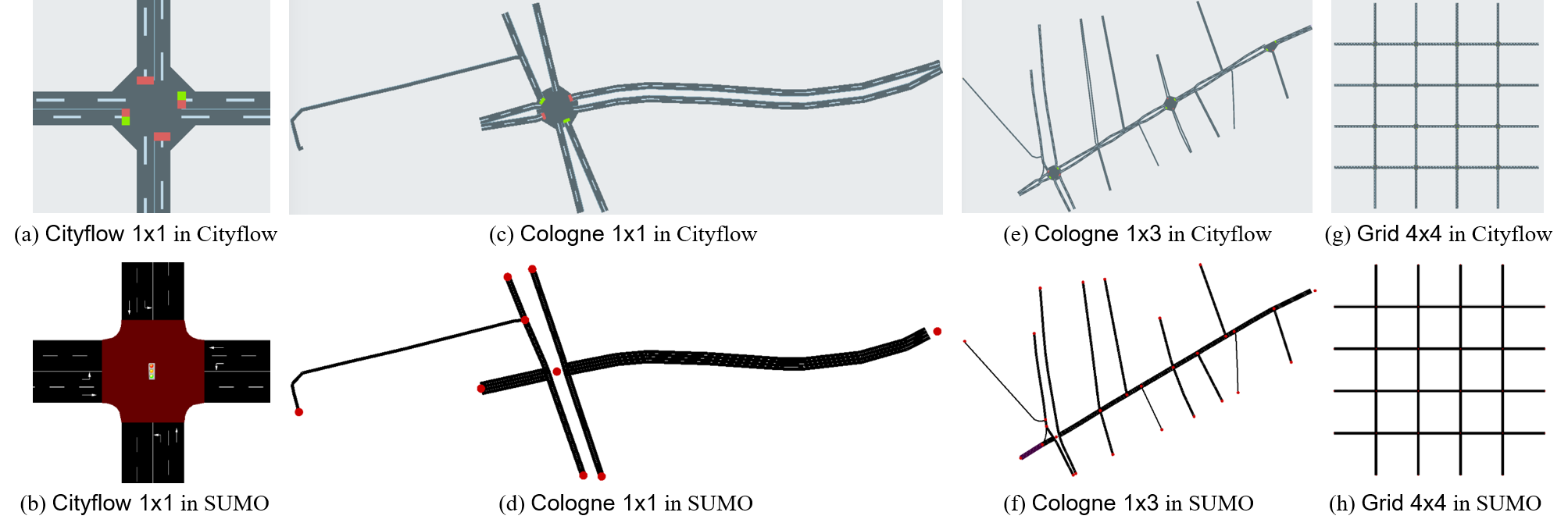
Figure 5: Road networks in different simulators for calibration

A.5 Calibration Steps

To validate the performance of the algorithms are consistent in both SUMO and CityFlow, we calibrate the simulators in the following aspects:  
$\bullet$ Calibration from SUMO to CityFlow: To make the conversion of complex networks from SUMO compatible with CityFlow, we redesign the original convert files from  zhang2019cityflow with the following: (1) For those .rou files in SUMO that only specify source and destination intersections and ignore roads that would be passing, the router command line in SUMO should be applied to generate full routes before converting it into CityFlow’s .json traffic flow file. (2) We treat all the intersections without traffic signals in SUMO as “virtual” nodes in CityFlow’s .json road network file. (3) We keep the time interval the same for red and yellow signals in SUMO and CityFlow. (4) SUMO has a feature of the dynamic routing of vehicles that CityFlow does not have, currently all the simulation under SUMO in LibSignal disables the dynamic routing.  
$\bullet$ Calibration from CityFlow to SUMO: The vehicles in CityFlow’s traffic flow file need to be sorted according to their departure time because the SUMO traffic file defaults to the depart time of the preceding vehicle earlier than the following vehicle.

Table 7: Performance of agents in CityFlow and SUMO on additional datasets that are not shown in Section 4.2 with best and second best performance highlighted.

Network	Cityflow 1x1(Config2)
Simulator	CityFlow				SUMO
Metric	Travel Time	Queue	Delay	Throughput	Travel Time	Queue	Delay	Throughput
FixedTime(t_fixed=10)	702.0847	90.3417	4.3542	914	444.5625	74.9	4.095	832
FixedTime(t_fixed=30)	305.9428	62.9361	4.3038	1246	181.3847	42.9972	4.2947	1310
MaxPressurre	91.4333	11.3806	4.5774	1388	85.7407	8.7333	4.1472	1377
SOTL	116.2653	20.0139	3.6794	1381	96.8388	13.2667	3.1959	1371
IDQN	79.6013	7.5806	0.4253	1390	78.0051	5.8111	0.3648	1379
MAPG	262.1785	75.3056	0.6467	1237	125.3895	61.075	0.5812	955
IPPO	733.7248	130.7694	0.6963	748	90.9229	10.6	0.4447	1375
PressLight	84.7516	9.2889	0.4454	1385	85.873	8.9639	0.4318	1378
Network	Cityflow 1x1(Config3)
Simulator	CityFlow				SUMO
Metric	Travel Time	Queue	Delay	Throughput	Travel Time	Queue	Delay	Throughput
FixedTime(t_fixed=10)	461.2692	33.5944	2.3989	531	284.4235	29.9806	2.2208	503
FixedTime(t_fixed=30)	228.8520	24.0667	2.7021	659	173.1985	21.3167	2.8096	680
MaxPressurre	69.7295	2.2250	1.8415	729	69.9601	1.6167	1.4375	726
SOTL	89.2005	5.5556	1.8778	729	84.9169	4.4556	1.7441	722
IDQN	66.9865	1.6833	0.1816	730	68.7369	1.2556	0.1396	726
MAPG	183.2719	25.7778	0.4086	651	115.5654	26.3361	0.3421	543
IPPO	79.4778	3.8333	0.2672	729	78.8072	3.0500	0.2373	726
PressLight	67.4899	1.8861	0.1945	731	73.4509	2.4250	0.2169	723
Network	Cityflow 1x1(Config4)
Simulator	CityFlow				SUMO
Metric	Travel Time	Queue	Delay	Throughput	Travel Time	Queue	Delay	Throughput
FixedTime(t_fixed=10)	686.7469	96.7222	4.4683	925	469.5721	81.7778	4.0367	811
FixedTime(t_fixed=30)	339.3052	63.7750	4.4226	1290	204.3520	51.7611	4.5938	1358
MaxPressurre	136.5470	31.9083	5.1600	1556	98.8589	17.3444	4.6113	1602
SOTL	158.4722	40.2611	4.5164	1562	113.0794	23.7389	3.7165	1587
IDQN	101.9282	18.7278	0.5685	1614	90.0737	12.8278	0.4912	1614
MAPG	435.5595	77.6861	0.6195	1179	137.0363	78.4028	0.6875	1130
IPPO	226.4010	58.2306	0.6641	1453	115.8968	52.4528	0.4787	1037
PressLight	90.1724	13.2667	0.4820	1630	91.8277	13.7250	0.5153	1608
Network	HangZhou4x4
Simulator	CityFlow				SUMO
Metric	Travel Time	Queue	Delay	Throughput	Travel Time	Queue	Delay	Throughput
FixedTime(t_fixed=10)	689.0221	13.9837	0.9636	2385	535.0060	7.9405	2.1130	2495
FixedTime(t_fixed=30)	575.5565	12.3694	1.8439	2645	580.5826	10.3816	2.4246	2355
MaxPressurre	365.0634	3.5972	1.7891	2928	350.4125	1.2870	0.9678	2732
SOTL	354.1250	2.7229	1.0208	2916	386.7881	3.3717	1.4937	2695
IDQN	322.9068	1.2141	0.0679	2929	341.8509	1.2097	0.0689	2730
MAPG	782.3319	24.0474	0.1406	2331	436.2691	25.1415	0.2374	1442
IPPO	727.9460	15.5786	0.1068	2306	418.0365	7.2328	0.1560	2496
PressLight	329.7855	1.6380	0.0841	2932	354.0689	1.4884	0.0803	2728
Colight	331.4348	1.7658	0.0906	2931	343.4998	1.3083	0.0714	2733
Network	Manhattan7x28
Simulator	CityFlow				SUMO
Metric	Travel Time	Queue	Delay	Throughput	Travel Time	Queue	Delay	Throughput
FixedTime(t_fixed=10)	1575.7847	20.7651	1.2703	7531	953.9797	19.3563	1.4353	2123
FixedTime(t_fixed=30)	1582.1030	22.3561	1.6659	7801	1144.1702	20.2811	1.8234	2379
MaxPressurre	1335.7877	17.3380	1.3035	9745	797.4855	15.2944	1.3298	4614
SOTL	1612.2468	23.6984	1.4968	8244	869.6206	17.8344	1.4543	3010
IDQN	1319.4959	17.4697	0.0916	9035	-	-	-	-
MAPG	1586.3388	21.2705	0.1159	7481	-	-	-	-
IPPO	1468.4135	19.4304	0.1130	8300	-	-	-	-
PressLight	1338.7183	18.1332	0.0961	9123	-	-	-	-
CoLight	1493.4200	19.5024	0.1007	8287	-	-	-	-

^∗ Results shown as (-) indicate that no RL methods can be trained within acceptable time and resource
in SUMO in Manhattan’s road network.

A.6 Supplementary Results

We conduct experiments on all nine datasets and also provide results of the best episode, full converge curves and standard deviations of the performance on the four datasets in full paper.

A.6.1 Other comparison studies on datasets not shown in full paper

Table 7 shows the result of performance on the other five datasets. It shows PressLight and IDQN are the most stable algorithms at the most of the times.

A.6.2 Converge curve of Table 4

Fig 6 shows the full converge curve of 2000 episodes for IPPO and MAPG agents. The result shows that comparing to Q-learning agents, Actor-Critic agents are hard to converge, on some large or complex datasets, converge time needed are more than ten times of Q-learning methods.

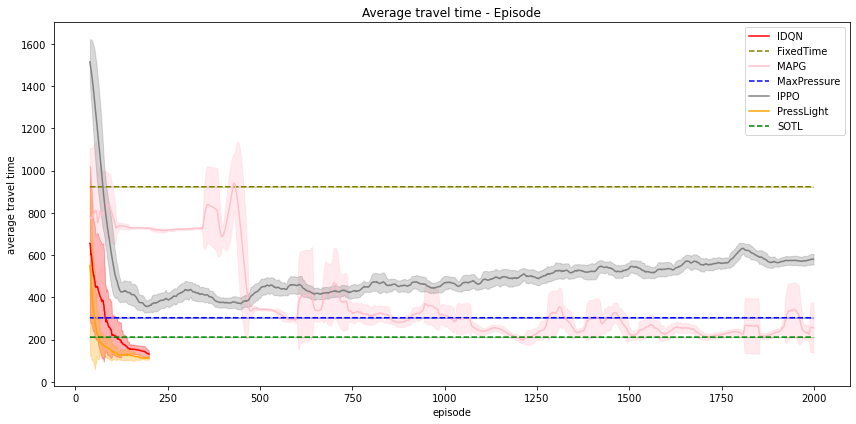
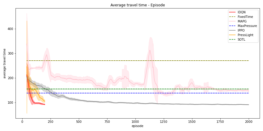
(a) CityFlow1x1 in CityFlow	(b) CityFlow1x1 in SUMO
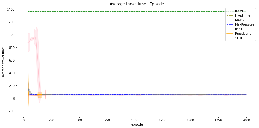
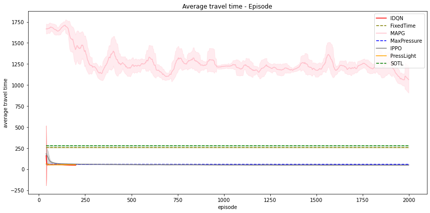
(c) Cologne1x1 in CityFlow	(d) Cologne1x1 in SUMO
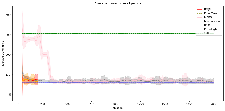
(e) Cologne1x3 in CityFlow	(f) Cologne1x3 in SUMO
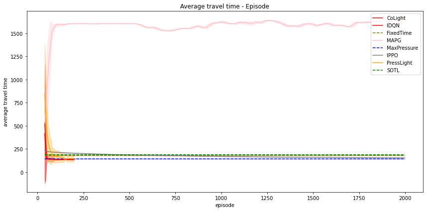
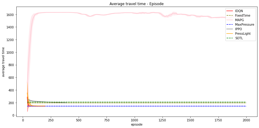
(g) Grid4x4 in CityFlow	(h) Grid4x4 in SUMO

Figure 6: Full converge curve of Table 4

A.6.3 Result of best episode

Table 8 gives the episode number of all datasets. It supports the conclusion that PressLight, followed by IDQN, have the best sample efficiency compared with other algorithms.

Table 8: The episode of best results for different agents w.r.t. different methods

Network	Simulator	IDQN	MAPG	IPPO	PressLight
Cityflow1x1	CityFlow	193	1205	185	197
	SUMO	187	188	194	185
Cologne1x1	CityFlow	95	1870	172	101
	SUMO	189	1992	346	193
Cologne1x3	CityFlow	133	597	1977	159
	SUMO	177	30	195	164
Grid4x4	CityFlow	163	6*	172	172
	SUMO	186	2*	188	143

^∗ Though MAPG and IPPO has the best results in the first few episodes,
their performances are still worse than the other agents.

A.6.4 Performance on benchmark with standard deviations

Table 9 shows the standard deviation of the performance on the four datasets in full paper.

Table 9: The standard deviations of Table 4

Network	Cityflow 1x1
Simulator	CityFlow				SUMO
Metric	Travel Time	Queue	Delay	Throughput	Travel Time	Queue	Delay	Throughput
IDQN	9.474	2.5995	0.0221	3.0496	2.507	0.6804	0.4424	0.0092
MAPG	10.746	0.2149	1.7188	0.0152	14.182	0.6544	0.4391	0.0031
IPPO	23.020	0.0011	1.9196	0.0055	12.179	0.0446	7.7187	0.015
PressLight	3.335	1.334	0.0127	2.5884	1.960	3.261	3.4475	0.0141
FRAP	3.0118	1.4411	1.5028	0.0106	0.6933	0.3848	0.4273	0.0095
Network	Cologne 1x1
Simulator	CityFlow				SUMO
Metric	Travel Time	Queue	Delay	Throughput	Travel Time	Queue	Delay	Throughput
IDQN	2.100	0.6913	0.7502	0.0095	0.144	0.6317	0.3986	0.0087
MAPG	2.186	0.0359	0.2659	0.0072	12.283	0.0088	0.0744	0.0001
IPPO	28.048	0.0003	0.0495	0.0015	0.950	0.0013	0.1982	0.0008
PressLight	2.274	0.3753	0.3161	0.0066	0.767	0.6011	0.6375	0.0106
Network	Cologne 1x3
Simulator	CityFlow				SUMO
Metric	Travel Time	Queue	Delay	Throughput	Travel Time	Queue	Delay	Throughput
IDQN	5.891	0.9075	0.1778	0.0053	0.875	0.0711	0.0111	0.0017
MAPG	2.883	0.0637	0.1467	0.0047	15.494	3.5459	0.5764	0.0134
IPPO	0.950	0.0	0.0159	0.002	4.107	0.0002	0.1743	0.0078
PressLight	0.619	0.124	0.0405	0.0026	4.982	2.3948	0.798	0.0123
Network	Grid4x4
Simulator	CityFlow				SUMO
Metric	Travel Time	Queue	Delay	Throughput	Travel Time	Queue	Delay	Throughput
IDQN	2.006	0.0117	0.0006	0.0	0.795	0.1733	0.0098	0.0005
MAPG	13.330	1.1346	0.071	0.0044	5.420	3.6906	0.2473	0.0049
IPPO	2.432	0.0003	0.0495	0.0015	3.465	0.0004	0.0346	0.0004
PressLight	0.880	0.0491	0.0022	0.0	0.636	0.1045	0.0132	0.0003
CoLight	0.8315	0.0161	0.0009	0.0	1.1633	0.621	0.0384	0.0017

A.7 Extension to Other Simulators

LibSignal is a cross-simulator library for traffic control tasks. Currently, we support the most commonly used CityFlow and SUMO simulators, and our library is open to other new simulation environments. CBEngine is a new simulator that served as the simulation environment in the KDD Cup 2021 City Brain Challenge  and is designed for executing traffic control tasks on large traffic networks. We integrate this new simulator into our traffic control framework to extend LibSignal’s usage in other simulation environments. We show the result of MaxPressure, SOTL, FixedTime, and IDQN’ performance under CBEngine in Table 10

Table 10: Performance on CBEngine simulator

CityFlow1x1	FixedTime	MaxPressure	SOTL	IDQN
Avg. Travel Time	654.4848	150.7677	96.0025	84.5404

A.8 Hyperparameters

Table 11 provides the parameters of each algorithm, training environment, and hardware parameters on the server.

Table 11: Hyperparameters of models, servers and training

Model Parameters
FixedTime	t_fixed	30	buffer_size	0	learning_rate	0	learning_start	0
	update_model_rate	0	update_target_rate	0	save_rate	0	train_model	false
	test_model	true	one_hot	false	phase	false	episodes	1
MaxPressure	t_min	10	buffer_size	0	learning_rate	0	learning_start	0
	update_model_rate	0	update_target_rate	0	save_rate	0	train_model	false
	test_model	true	one_hot	false	phase	false	episodes	1
SOTL	t_min	5	min_green_vehicle	3	max_red_vehicle	6	buffer_size	0
	learning_rate	0	learning_start	0	update_model_rate	0	update_target_rate	0
	save_rate	0	train_model	false	test_model	true	one_hot	false
	phase	false	episodes	1
IDQN	learning_rate	0.001	learning_start	1000	graphic	false	buffer_size	5000
	batch_size	64	episodes	200	epsilon	0.1	epsilon_decay	0.995
	epsilon_min	0.01	update_model_rate	1	update_target_rate	10	save_rate	20
	one_hot	true	phase	true	gamma	0.95	steps	3600
	test_steps	3600	vehicle_max	1	grad_clip	5	train_model	false
	test_model	true	action_interval	10
MAPG	tau	0.01	learning_rate	0.001	learning_start	5000	graphic	false
	buffer_size	10000	batch_size	256	episodes	2000	epsilon	0.5
	epsilon_decay	0.99	epsilon_min	0.01	update_model_rate	30	update_target_rate	30
	save_rate	1000	one_hot	FLASE	phase	false	gamma	0.95
	steps	3600	test_steps	3600	vehicle_max	1	grad_clip	5
	train_model	false	test_model	true	action_interval	10
IPPO	learning_rate	0.0001	learning_start	-1	graphic	false	buffer_size	5000
	batch_size	64	episodes	2000	epsilon	0.1	epsilon_decay	0.995
	epsilon_min	0.01	update_model_rate	1	update_target_rate	10	save_rate	1000
	one_hot	true	phase	true	gamma	0.95	steps	3600
	test_steps	3600	vehicle_max	1	grad_clip	5	train_model	false
	test_model	true	action_interval	10
PressLight	d_dense	20	n_layer	2	normal_factor	20	patience	10
	learning_rate	0.001	learning_start	1000	graphic	false	buffer_size	5000
	batch_size	64	episodes	200	epsilon	0.1	epsilon_decay	0.995
	epsilon_min	0.01	update_model_rate	1	update_target_rate	10	save_rate	20
	one_hot	true	phase	true	gamma	0.95	steps	3600
	test_steps	3600	vehicle_max	1	grad_clip	5	train_model	false
	test_model	true	action_interval	10
FRAP	d_dense	20	n_layer	2	one_hot	false	phase	true
	learning_rate	0.001	learning_start	1000	graphic	false	buffer_size	5000
	rotation	true	conflict_matrix	true	merge	multiply	demand_shape	1
	batch_size	64	episodes	200	epsilon	0.1	epsilon_decay	0.995
	epsilon_min	0.01	update_model_rate	1	update_target_rate	10	save_rate	20
	test_steps	3600	test_model	true	action_interval	10	train_model	true
MPLight	d_dense	20	n_layer	2	one_hot	false	phase	true
	learning_rate	0.001	learning_start	-1	graphic	false	buffer_size	10000
	rotation	true	conflict_matrix	true	merge	multiply	demand_shape	1
	batch_size	32	episodes	200	eps_start	1	eps_end	0
	eps_decay	220	target_update	500	gamma	0.99	save_rate	20
	test_steps	3600	test_model	true	action_interval	10	train_model	true
CoLight	neighbor_num	4	neighbor_edge_num	4	n_layer	1	input_dim	[128,128]
	output_dim	[128,128]	node_emb_dim	[128,128]	num_heads	[5,5]	node_layer_dims_each_head	[16,16]
	output_layers	[]	learning_rate	0.001	learning_start	1000	graphic	true
	buffer_size	5000	batch_size	64	episodes	200	epsilon	0.8
	epsilon_decay	0.9995	epsilon_min	0.01	update_model_rate	1	update_target_rate	10
	save_rate	20	one_hot	true	phase	false	gamma	0.95
	steps	3600	test_steps	3600	vehicle_max	1	grad_clip	5
	train_model	false	test_model	true	action_interval	10
Server Parameters
pc1	cpu	Intel(R) Xeon(R) Platinum 8163 CPU @ 2.50GHz			cpu cores	24	mem total	251.55GB
pc2	cpu	Intel(R) Xeon(R) Platinum 8124M CPU @ 3.00GHz			cpu cores	18	mem total	251.54GB
Training Parameters
thread	4	ngpu	-1	action_pattern		"set"	if_gui	true
debug	false	interval	1	savereplay		true	rltrafficlight	true

References

- (1) Reinforcement learning for traffic signal control. https://traffic-signal-control.github.io/. Accessed: 2022-05-22.
- (2) James Ault and Guni Sharon. Reinforcement learning benchmarks for traffic signal control. In Thirty-fifth Conference on Neural Information Processing Systems Datasets and Benchmarks Track (Round 1), 2021.
- (3) Greg Brockman, Vicki Cheung, Ludwig Pettersson, Jonas Schneider, John Schulman, Jie Tang, and Wojciech Zaremba. Openai gym, 2016.
- (4) Miaomiao Cao, Victor OK Li, and Qiqi Shuai. A gain with no pain: Exploring intelligent traffic signal control for emergency vehicles. IEEE Transactions on Intelligent Transportation Systems, 2022.
- (5) Chacha Chen, Hua Wei, Nan Xu, Guanjie Zheng, Ming Yang, Yuanhao Xiong, Kai Xu, and Zhenhui Li. Toward a thousand lights: Decentralized deep reinforcement learning for large-scale traffic signal control. In Proceedings of the AAAI Conference on Artificial Intelligence, volume 34, pages 3414–3421, 2020.
- (6) Tianshu Chu, Jie Wang, Lara Codecà, and Zhaojian Li. Multi-agent deep reinforcement learning for large-scale traffic signal control. IEEE Transactions on Intelligent Transportation Systems, 21(3):1086–1095, 2019.
- (7) François-Xavier Devailly, Denis Larocque, and Laurent Charlin. Ig-rl: Inductive graph reinforcement learning for massive-scale traffic signal control. IEEE Transactions on Intelligent Transportation Systems, 2021.
- (8) Nishant Kheterpal, Kanaad Parvate, Cathy Wu, Aboudy Kreidieh, Eugene Vinitsky, and Alexandre Bayen. Flow: Deep reinforcement learning for control in sumo. EPiC Series in Engineering, 2:134–151, 2018.
- (9) Pablo Alvarez Lopez, Michael Behrisch, Laura Bieker-Walz, Jakob Erdmann, Yun-Pang Flötteröd, Robert Hilbrich, Leonhard Lücken, Johannes Rummel, Peter Wagner, and Evamarie Wießner. Microscopic traffic simulation using sumo. In 2018 21st international conference on intelligent transportation systems (ITSC), pages 2575–2582. IEEE, 2018.
- (10) Jinming Ma and Feng Wu. Feudal multi-agent deep reinforcement learning for traffic signal control. In Proceedings of the 19th International Conference on Autonomous Agents and Multiagent Systems (AAMAS), pages 816–824, 2020.
- (11) Afshin Oroojlooy, Mohammadreza Nazari, Davood Hajinezhad, and Jorge Silva. Attendlight: Universal attention-based reinforcement learning model for traffic signal control. Advances in Neural Information Processing Systems, 33:4079–4090, 2020.
- (12) Xue Bin Peng, Marcin Andrychowicz, Wojciech Zaremba, and Pieter Abbeel. Sim-to-real transfer of robotic control with dynamics randomization. In 2018 IEEE international conference on robotics and automation (ICRA), pages 3803–3810. IEEE, 2018.
- (13) Majid Raeis and Alberto Leon-Garcia. A deep reinforcement learning approach for fair traffic signal control. In 2021 IEEE International Intelligent Transportation Systems Conference (ITSC), pages 2512–2518. IEEE, 2021.
- (14) Faizan Rasheed, Kok-Lim Alvin Yau, Rafidah Md Noor, Celimuge Wu, and Yeh-Ching Low. Deep reinforcement learning for traffic signal control: A review. IEEE Access, 8:208016–208044, 2020.
- (15) Stefano Giovanni Rizzo, Giovanna Vantini, and Sanjay Chawla. Reinforcement learning with explainability for traffic signal control. In 2019 IEEE Intelligent Transportation Systems Conference (ITSC), pages 3567–3572. IEEE, 2019.
- (16) Stefano Giovanni Rizzo, Giovanna Vantini, and Sanjay Chawla. Time critic policy gradient methods for traffic signal control in complex and congested scenarios. In Proceedings of the 25th ACM SIGKDD International Conference on Knowledge Discovery & Data Mining, pages 1654–1664, 2019.
- (17) Toan V. Tran, Thanh-Nam Doan, and Mina Sartipi. Tslib: A unified traffic signal control framework using deep reinforcement learning and benchmarking. In 2021 IEEE International Conference on Big Data (Big Data), pages 1739–1747, 2021.
- (18) Min Wang, Libing Wu, Jianxin Li, and Liu He. Traffic signal control with reinforcement learning based on region-aware cooperative strategy. IEEE Transactions on Intelligent Transportation Systems, 2021.
- (19) Hua Wei, Chacha Chen, Guanjie Zheng, Kan Wu, Vikash Gayah, Kai Xu, and Zhenhui Li. Presslight: Learning max pressure control to coordinate traffic signals in arterial network. In Proceedings of the 25th ACM SIGKDD International Conference on Knowledge Discovery & Data Mining, pages 1290–1298, 2019.
- (20) Hua Wei, Nan Xu, Huichu Zhang, Guanjie Zheng, Xinshi Zang, Chacha Chen, Weinan Zhang, Yanmin Zhu, Kai Xu, and Zhenhui Li. Colight: Learning network-level cooperation for traffic signal control. In Proceedings of the 28th ACM International Conference on Information and Knowledge Management, pages 1913–1922, 2019.
- (21) Hua Wei, Guanjie Zheng, Vikash Gayah, and Zhenhui Li. A survey on traffic signal control methods. arXiv preprint arXiv:1904.08117, 2019.
- (22) Hua Wei, Guanjie Zheng, Vikash Gayah, and Zhenhui Li. Recent advances in reinforcement learning for traffic signal control: A survey of models and evaluation. ACM SIGKDD Explorations Newsletter, 22(2):12–18, 2021.
- (23) Hua Wei, Guanjie Zheng, Huaxiu Yao, and Zhenhui Li. Intellilight: A reinforcement learning approach for intelligent traffic light control. In Proceedings of the 24th ACM SIGKDD International Conference on Knowledge Discovery & Data Mining, pages 2496–2505, 2018.
- (24) Libing Wu, Min Wang, Dan Wu, and Jia Wu. Dynstgat: Dynamic spatial-temporal graph attention network for traffic signal control. In Proceedings of the 30th ACM International Conference on Information & Knowledge Management, pages 2150–2159, 2021.
- (25) Yuanhao Xiong, Guanjie Zheng, Kai Xu, and Zhenhui Li. Learning traffic signal control from demonstrations. In Proceedings of the 28th ACM International Conference on Information and Knowledge Management, pages 2289–2292, 2019.
- (26) Bingyu Xu, Yaowei Wang, Zhaozhi Wang, Huizhu Jia, and Zongqing Lu. Hierarchically and cooperatively learning traffic signal control. In Proceedings of the AAAI Conference on Artificial Intelligence, volume 35, pages 669–677, 2021.
- (27) Kok-Lim Alvin Yau, Junaid Qadir, Hooi Ling Khoo, Mee Hong Ling, and Peter Komisarczuk. A survey on reinforcement learning models and algorithms for traffic signal control. ACM Computing Surveys (CSUR), 50(3):1–38, 2017.
- (28) Chia-Cheng Yen, Dipak Ghosal, Michael Zhang, and Chen-Nee Chuah. A deep on-policy learning agent for traffic signal control of multiple intersections. In 2020 IEEE 23rd International Conference on Intelligent Transportation Systems (ITSC), pages 1–6. IEEE, 2020.
- (29) Xinshi Zang, Huaxiu Yao, Guanjie Zheng, Nan Xu, Kai Xu, and Zhenhui Li. Metalight: Value-based meta-reinforcement learning for traffic signal control. In Proceedings of the AAAI Conference on Artificial Intelligence, volume 34, pages 1153–1160, 2020.
- (30) Huichu Zhang, Siyuan Feng, Chang Liu, Yaoyao Ding, Yichen Zhu, Zihan Zhou, Weinan Zhang, Yong Yu, Haiming Jin, and Zhenhui Li. Cityflow: A multi-agent reinforcement learning environment for large scale city traffic scenario. In The world wide web conference, pages 3620–3624, 2019.
- (31) Huichu Zhang, Chang Liu, Weinan Zhang, Guanjie Zheng, and Yong Yu. Generalight: Improving environment generalization of traffic signal control via meta reinforcement learning. In Proceedings of the 29th ACM International Conference on Information & Knowledge Management, pages 1783–1792, 2020.
- (32) Wenshuai Zhao, Jorge Peña Queralta, and Tomi Westerlund. Sim-to-real transfer in deep reinforcement learning for robotics: a survey. In 2020 IEEE Symposium Series on Computational Intelligence (SSCI), pages 737–744. IEEE, 2020.
- (33) Guanjie Zheng, Yuanhao Xiong, Xinshi Zang, Jie Feng, Hua Wei, Huichu Zhang, Yong Li, Kai Xu, and Zhenhui Li. Learning phase competition for traffic signal control. In Proceedings of the 28th ACM International Conference on Information and Knowledge Management, pages 1963–1972, 2019.
- (34) Guanjie Zheng, Xinshi Zang, Nan Xu, Hua Wei, Zhengyao Yu, Vikash Gayah, Kai Xu, and Zhenhui Li. Diagnosing reinforcement learning for traffic signal control, 2019.