Fully implicit frictional dynamics with soft constraints

Abstract.

Dynamics simulation with frictional contacts is important for a wide range of applications, from cloth simulation to object manipulation. Recent methods using smoothed friction forces have enabled robust and differentiable simulation of elastodynamics with friction. However, the resulting frictional behaviors can be qualitatively inaccurate and may not converge to analytic solutions. Here we propose an alternative, fully implicit, formulation for simulating elastodynamics subject to frictional contacts with realistic friction behavior. Furthermore, we demonstrate how higher-order time integration can be used in our method, as well as in incremental potential methods. We develop an inexact Newton method with forward-mode automatic differentiation that simplifies the implementation and improves performance. Finally, we show how our method can be extended to respond to volume changes using a unified penalty function derived from first principles and capable of emulating compressible as well as nearly incompressible media.

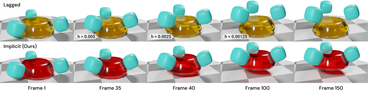
[Three soft pads picking up an upside-down bowl]Renders of three soft pads lifting an upside-down bowl

Figure 1. An upside-down bowl is lifted using 3 soft pads via friction. The bowl is simulated using the lagged friction model from Li et al. (2020) (top row) and our fully implicit method (Eq. (23), bottom row). The chosen frames between 1 and 150, are frames 35, 40 and 100, at which point the bowl slips out for time steps $h=0.005$ s, $0.0025$ s, and $0.00125$ s respectively for the lagged method. Using fully implicit integration, the bowl sticks even at the largest time step $h=0.005$ s as shown. For the pads, $\rho=1000$ kg/m³ (density), $E=600$ KPa (Young’s modulus), and $\nu=0.49$ (Poisson ratio). For the bowl, $\rho=400$ kg/m³, $E=11000$ KPa and $\nu=0.1$. The friction coefficient is set to $\mu=0.65$ between the two. See Figure 5 for the plot of the bowl height in all tested configurations.

1. Introduction

Modern simulation pipelines in computer graphics and engineering involve contact handling. This ensures that simulated objects do not interpenetrate each other as they interact. During this interaction, friction ensures that solid objects are held in place or are otherwise limited in how far they move. This work focuses on the accuracy and effectivity of smooth friction models.

In recent years we have seen a resurgence of promising work in developing more robust methods for simulating frictional contact in computer graphics. This problem is particularly difficult since friction and contact cannot be simultaneously described by a single energy potential (De Saxcé and Feng, 1998). This precludes formulating the frictional contact problem as a single energy minimization. However, energy minimization used for solving discretized ordinary differential equations (ODEs) remains a popular choice in graphics, due to its flexibility and robustness characteristics. Unfortunately, optimization based solvers used for dynamics equations require specialized algorithms for handling frictional contacts, which necessarily produces drawbacks in accuracy or robustness.

In this work, we demonstrate the failure cases in popular optimization based frictional contact solvers and propose an alternative method for solving elastodynamic problems with frictional contacts that is simple to implement and accurate in comparison. By solving nonlinear equations of motion directly via root finding, our method does not require additional iterations or specialized mechanisms for coupling friction, contact and elasticity to achieve reasonable accuracy.

Frictional contact is traditionally modelled as a non-smooth problem requiring sophisticated tools. In particular, non-smooth integrators, root finding or optimization techniques are needed for handling inclusion terms in the mathematical model. This drastically complicates the problem and substantially limits the number of solution approaches. While non-smoothness is required to guarantee absolute sticking, it is not generally necessary if simulations are limited in time. In fact, when observed on a microscale, even dry friction responds continuously to changes in velocity (Wojewoda et al., 2008). Accordingly, we adopt a smooth friction formulation, and show that when applied correctly in dynamics equations it can produce predictable sticking. In contrast, popular friction models like lagged friction, cause inaccurate and time step dependent sticking behavior.

To our knowledge this work is the first to demonstrate the importance of evaluating the sliding basis (defined in Section 3.3) and contact forces implicitly for accurate friction simulation.

Finally, to maintain smoothness of the entire problem we employ a penalty force for contact resolution and a smooth implicit surface model proposed by Larionov et al. (2021) for representing the contact surface. We also show how additional soft constraints can be added to the system for controlling the volume of an object.

Maintaining smoothness of the entire system makes it easier to solve and allows derivatives to be propagated through each step of the simulation. However, full differentiable simulation is outside the scope of this work.

In summary, we propose

• A fully implicit method for simulating hyperelastic objects producing accurate friction behavior.

• Accurate high-order time integration applied to frictional contact problems for our fully implicit method as well as popular lagged friction formulations.

• An adaptive penalty stiffening strategy for effectively resolving interpenetrations with penalty-based contact methods.

• A physically-based volume change penalty for controlling compressibility in compressible and nearly incompressible regions.

Furthermore, to better characterize the instability of single point frictional contacts, we present an eigen-analysis of a 2D point contact subject to friction in Appendix A.

2. Related Work

Simulating the dynamics of deformable elastic objects (Terzopoulos et al., 1987) and cloth (Baraff and Witkin, 1998) has been an active area of research in graphics for decades. Methods requiring accuracy often reach for a finite element method (FEM) (Sifakis and Barbic, 2012), while methods aiming for performance reach for position-based techniques (Müller et al., 2007; Macklin et al., 2016; Bender et al., 2017), or projective-dynamics (Bouaziz et al., 2014). Our work targets simulation accuracy, and thus stays close to the tried and tested FEM.

Frictional Contact

In recent years, lots of attention has been dedicated towards robust and accurate contact and friction solutions. Earlier works in graphics developed non-smooth methods to resolve contact and friction forces at the end of the time step obtaining solutions faithful to the Coulomb model. Kaufman et al. (2008) proposed a predictor-corrector method to solve for friction and contact separately from elasticity equations. This was later extended to full FEM simulations (Larionov et al., 2021) while maintaining the decoupling. Other methods reformulate the problem as a non-smooth root finding problem (Bertails-Descoubes et al., 2011; Daviet et al., 2011; Li et al., 2018; Macklin et al., 2019) or using proximal algorithms (Erleben, 2017). More recently, more attention was brought towards modelling friction as a smoothly changing force at the stick-slip limit (Geilinger et al., 2020; Li et al., 2020). This allows each simulation step to remain differentiable. Geilinger et al. (2020) favored a more traditional root-finding solver combining friction and contact forces with elastic equations of motion. In contrast, Li et al. (2020) proposed a robust optimization framework to solve for contact and lagged friction forces. Unfortunately, even with multiple iterations, the lagged friction approach does not converge to an accurate friction solution, which is especially noticeable in sticking configurations close to the slip threshold. Furthermore, their proposed method for higher-order integration is not applied to the contact solve causing instabilities. In this work, we demonstrate and address these shortcomings using a solution that favors friction accuracy at the cost of some robustness, while maintaining smoothness of the system.

Higher-order integrators for contact problems

Most contact formulations, especially those formulated in terms of constraints, intrinsically rely on a particular choice of time discretization, which is usually backward Euler (BE). However, the highly dissipative characteristics of BE have motivated the use of higher-order schemes like TR-BDF2 or SDIRK2, which preserve high energy dynamics while maintaining stability (Ascher et al., 2022; Löschner et al., 2020). A benefit of smooth contact models based on penalty or barrier functions is that both normal and friction forces are defined with explicit formulas, as opposed to implicitly defined through constraints. This makes it possible to apply higher-order integrators directly, as demonstrated by Geilinger et al. (2020) for BDF2. Li et al. (2020) applied trapezoid rule (TR), however it is only applied to non-contact forces, which causes stability issues. Brown et al. (2018) focus on first-order methods and apply TR-BDF2 to a non-smooth optimization-based contact model with lagged friction, though this has unclear implications for high-accuracy second-order methods. In contrast to previous work, our approach is the first to incorporate contact, friction, elasticity and damping in a single fully implicit system evaluated using objects with deforming contact surfaces. We demonstrate the use of BDF2 and SDIRK2 applied to our formulation in Section 5.3.1.

Volume preservation

Many solids exhibit volume preserving behavior. We focus primarily on inflated objects like tires, sports equipment (e.g. sports balls), as well as nearly incompressible objects like the human body. Inflated objects are typically simulated using soft constraints (Bender et al., 2017), where the volume change of an object is penalized. These methods are effective, however, their physical accuracy is rarely questioned. Incompressible or nearly-incompressible materials are often modeled with stiff Poisson’s ratios (Smith et al., 2018) or hard volume preservation constraints (Sheen et al., 2021). In contrast, we propose a unified physically-based penalty formulation for volume preservation that models both compressible and nearly-incompressible objects using a single penalty controlled by a physical compression coefficient.

3. Method

Here we develop the equations of motion involved in solving for the motion of solid objects subject to frictional contacts.

A set of generalized coordinates $\boldsymbol{\mathrm{q}}(t)\in\mathbb{R}^{m}$ (e.g. stacked vertex positions of an FEM mesh), represents a system of solids moving through time $t$. A sparse symmetric positive definite (SPD) $m\times m$ matrix $\boldsymbol{\mathrm{M}}$ denotes generalized mass. In the following we omit the time derivative for brevity, but later reintroduce it when discussing time discretization schemes.

Using dot notation to denote time derivatives and with generalized velocities $\boldsymbol{\mathrm{v}}=\dot{\boldsymbol{\mathrm{q}}}$ we can write the force balance equation as

(1) $$\boldsymbol{\mathrm{M}}\dot{\boldsymbol{\mathrm{v}}} =\boldsymbol{\mathrm{f}}(\boldsymbol{\mathrm{q}},\boldsymbol{\mathrm{v}})$$

(2) $$\boldsymbol{\mathrm{f}}(\boldsymbol{\mathrm{q}},\boldsymbol{\mathrm{v}}) =\boldsymbol{\mathrm{f}}_{e}(\boldsymbol{\mathrm{q}})+\boldsymbol{\mathrm{f}}_{d}(\boldsymbol{\mathrm{q}},\boldsymbol{\mathrm{v}})+\boldsymbol{\mathrm{f}}_{c}(\boldsymbol{\mathrm{q}})+\boldsymbol{\mathrm{f}}_{f}(\boldsymbol{\mathrm{q}},\boldsymbol{\mathrm{v}})+\boldsymbol{\mathrm{f}}_{g}(\boldsymbol{\mathrm{q}}),$$

where $\boldsymbol{\mathrm{f}}_{e}$ are elastic forces, $\boldsymbol{\mathrm{f}}_{d}$ are damping forces, $\boldsymbol{\mathrm{f}}_{c}$ are contact forces, $\boldsymbol{\mathrm{f}}_{f}$ is friction, and $\boldsymbol{\mathrm{f}}_{g}$ are external forces such as gravity.

3.1. Elasticity and Damping

Elastic forces are typically derived from a configuration dependent energy potential $W(\boldsymbol{\mathrm{q}})$ as

$$\boldsymbol{\mathrm{f}}_{e}(\boldsymbol{\mathrm{q}})=-\frac{\partial}{\partial\boldsymbol{\mathrm{q}}}W(\boldsymbol{\mathrm{q}}).$$

The elastic potential $W$ can be defined by the classic linear, neo-Hookean, StVK or Mooney-Rivlin models (Ciarlet, 1983), or even a data-driven model (Wang et al., 2011). We will focus on neo-Hookean materials for both solids and cloth. We then define the stiffness matrix $\boldsymbol{\mathrm{K}}(\boldsymbol{\mathrm{q}})=-\frac{\partial}{\partial\boldsymbol{\mathrm{q}}}\boldsymbol{\mathrm{f}}_{e}(\boldsymbol{\mathrm{q}})$, which dictates how resistant an object is to deformation. For nonlinear models like neo-Hookean elasticity, $\boldsymbol{\mathrm{K}}$ may be indefinite, which is important to know when picking an appropriate linear solver.

Damping forces are often defined by

$$\boldsymbol{\mathrm{f}}_{d}(\boldsymbol{\mathrm{q}},\boldsymbol{\mathrm{v}})=-\boldsymbol{\mathrm{D}}(\boldsymbol{\mathrm{q}})\boldsymbol{\mathrm{v}},$$

where $\boldsymbol{\mathrm{D}}$ is a symmetric matrix. We use the Rayleigh damping model for simplicity where $\boldsymbol{\mathrm{D}}=\alpha\boldsymbol{\mathrm{M}}+\beta\boldsymbol{\mathrm{K}}$ for some constants $\alpha,\beta\geq 0$.

3.2. Contact

Traditionally contact constraints have been formulated with a positivity constraint (strict or not) on some “gap” function $\boldsymbol{\mathrm{d}}(\boldsymbol{\mathrm{q}})$ that roughly determines how far objects are away from each other. This function $\boldsymbol{\mathrm{d}}$ may be closely related to a component-wise signed distance function, however, generally it merely needs to be continuous, monotonically increasing in the direction of separation, and constant at the surface. We define $d_{i}$ for each potential contact point $i$ such that $\boldsymbol{\mathrm{d}}=(d_{1},d_{2},\dots,d_{n})$ where $n$ is the total number of potential contacts. Here we use the contact model of Larionov et al. (2021), where surface vertices of one object are constrained to have non-negative potential values when evaluated against a smooth implicit function $\boldsymbol{\mathrm{d}}$ closely approximating the surface of another object. Interestingly, if we allow objects some small separation tolerance at equilibrium, we can reformulate this constraint as an equality constraint by using a soft-max (Geilinger et al., 2020) or a truncated log barrier (Li et al., 2020). These types of equality constraints greatly simplify the contact problem and have shown tremendous success in practice.

One disadvantage of log-barrier formulations is that the initial state must be free of collisions prior to the optimization step in order to avoid infinite energies and undefined derivatives. In the absence of thin features or risk of tunneling, it is sufficient to use a simple penalty function to resolve interpenetrating geometry. In this work we choose to use penalty-based contacts for simplicity, however, our formulation is fully compatible with a log-barrier method coupled with continuous collision detection (CCD) as proposed by Li et al. (2020). The idea is to help our solver guide interpenetrating meshes out of intersecting configurations. We define a cubic contact penalty by

$$b(x;\delta,\kappa)=\kappa\left\{\begin{array}[]{ll}-(x-\delta)^{3}&\text{ if }x<\delta\\ 0&\text{ otherwise,}\end{array}\right.$$

where $\delta>0$ is the thickness tolerance and $\kappa>0$ is a contact stiffness parameter that will need to be automatically increased to ensure that no surface vertices of one object are penetrating the implicit surface of another at the end of the time step. Here $b$ corresponds to the first non-zero term in the Taylor expansion of the truncated log-barrier used by Li et al. (2020), but unlike the log-barrier it is well-defined also for negative arguments. The penalty is applied to each contact point giving us an aggregate contact energy

$$W_{c}(\boldsymbol{\mathrm{d}})=\sum_{i=1}^{n}b(d_{i};\delta,\kappa).$$

Now the contact force can be written simply as the negative energy derivative

(3) $$\boldsymbol{\mathrm{f}}_{c}(\boldsymbol{\mathrm{q}})^{\top}=-\frac{\partial W_{c}}{\partial\boldsymbol{\mathrm{q}}}=\boldsymbol{\mathrm{\lambda}}(\boldsymbol{\mathrm{q}})^{\top}\frac{\partial\boldsymbol{\mathrm{d}}}{\partial\boldsymbol{\mathrm{q}}}, \boldsymbol{\mathrm{\lambda}}(\boldsymbol{\mathrm{q}})^{\top}=-\frac{\partial W_{c}}{\partial\boldsymbol{\mathrm{d}}}$$ where

is the stacked vector of contact force magnitudes. In effect our contact formulation enforces the equality constraint $W_{c}(\boldsymbol{\mathrm{d}}(\boldsymbol{\mathrm{q}}))=0$.

3.3. Friction

We define the contact Jacobian $\boldsymbol{\mathrm{J}}_{c}(\boldsymbol{\mathrm{q}})$ and tangent basis $\boldsymbol{\mathrm{B}}(\boldsymbol{\mathrm{q}})$ over all potential contact points as in (Larionov et al., 2021). Then $\boldsymbol{\mathrm{T}}(\boldsymbol{\mathrm{q}})=\boldsymbol{\mathrm{J}}_{c}(\boldsymbol{\mathrm{q}})^{\top}\boldsymbol{\mathrm{B}}(\boldsymbol{\mathrm{q}})$ is the $m\times n$ matrix defining the sliding basis (Li et al., 2020). In short, this matrix maps forces in contact space to generalized forces in configuration space.

We can now derive the smoothed friction force (Li et al., 2020; Geilinger et al., 2020) from first principles. For each contact $i$, the maximum dissipation principle (MDP) postulates that friction force ought to maximally oppose relative velocity

(4) $$\boldsymbol{\mathrm{f}}_{f,i}(\boldsymbol{\mathrm{v}};\mu)=\operatorname*{argmax}_{\|\boldsymbol{\mathrm{y}}\|\leq\mu\lambda_{i}}(-\bar{\boldsymbol{\mathrm{v}}}_{i}^{\top}\boldsymbol{\mathrm{y}}),$$

where $\mu$ is the coefficient of friction, which limits the friction force and $\bar{\boldsymbol{\mathrm{v}}}_{i}\in\mathbb{R}^{2}$ is the relative tangential velocity at contact point $i$. The contact force magnitude $\lambda_{i}$ is the $i$th element of $\boldsymbol{\mathrm{\lambda}}$ as defined in Eq. (3). We can solve Eq. (4) explicitly with an inclusion

(7) $$\boldsymbol{\mathrm{f}}_{f,i}(\boldsymbol{\mathrm{v}};\mu)\in-\mu\lambda_{i}\left\{\begin{array}[]{ll}\{\bar{\boldsymbol{\mathrm{v}}}_{i}/\|\bar{\boldsymbol{\mathrm{v}}}_{i}\|\}&\text{ if }\|\bar{\boldsymbol{\mathrm{v}}}_{i}\|>0\\ \{\boldsymbol{\mathrm{u}}\in\mathbb{R}^{2}\ :\ \|\boldsymbol{\mathrm{u}}\|\leq 1\}&\text{ otherwise}.\end{array}\right.$$

This is commonly referred to as Coulomb friction. Unfortunately, the non-smoothness around $\|\bar{\boldsymbol{\mathrm{v}}}_{i}\|=0$ calls for non-smooth optimization or root-finding techniques (Kaufman et al., 2008; Bertails-Descoubes et al., 2011; Erleben, 2017), making this problem numerically challenging. Another disadvantage of non-smoothness is that it greatly complicates differentiation of the solver, which can be critical for solving inverse problems efficiently. We opt to approximate Coulomb friction using a smoothed model (Li et al., 2020; Geilinger et al., 2020). Since most animations call for relatively short time frames, we typically do not require absolute sticking. Interestingly, smooth friction models have been proposed in older engineering literature (Kikuuwe et al., 2005; Wojewoda et al., 2008; Awrejcewicz et al., 2008) to improve hysteretic behavior and alleviate numerical difficulties. A simple smoothing of Eq. (7) can be written as

(8) $$\boldsymbol{\mathrm{f}}_{f,i}(\boldsymbol{\mathrm{v}};\mu)\approx-\mu\lambda_{i}\boldsymbol{\mathrm{\eta}}(\bar{\boldsymbol{\mathrm{v}}}_{i}),$$

where $\boldsymbol{\mathrm{\eta}}:\mathbb{R}^{2}\to\mathbb{R}^{2}$ defines the per-contact nonlinearity

(11) $$\boldsymbol{\mathrm{\eta}}(\bar{\boldsymbol{\mathrm{v}}}_{i})=s(\|\bar{\boldsymbol{\mathrm{v}}}_{i}\|)\left\{\begin{array}[]{ll}\bar{\boldsymbol{\mathrm{v}}}_{i}/\|\bar{\boldsymbol{\mathrm{v}}}_{i}\|&\text{ if }\|\bar{\boldsymbol{\mathrm{v}}}_{i}\|>0\\ 0&\text{ otherwise, }\end{array}\right.$$

and the function $s$ defines the pre-sliding transition. A suitable $C^{1}$ option for $s$ proposed by Li et al. (2020) is

(14) $$s_{a}(x;\epsilon)=\left\{\begin{array}[]{ll}\frac{2x}{\epsilon}-\frac{x^{2}}{\epsilon^{2}}&\text{ if }x<\epsilon\\ 1&\text{ otherwise. }\end{array}\right.$$

For a $C^{\infty}$ option, we can define

(15) $$s_{b}(x;\epsilon)=\frac{x}{x+\epsilon}.$$

Figure 2 illustrates how $s_{a}$ and $s_{b}$ behave for different values of the stick-slip parameter $\epsilon$. In our experiments, both functions produced accurate friction effects.

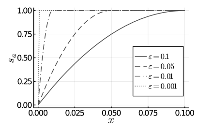
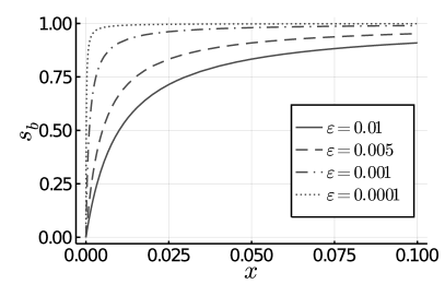
A series of plots of s_a for values between 0 and 1 plotted against x between 0 and 0.1 that become almost vertical near x = 0 and horizontal everywhere else. A series of plots of s_b for values between 0 and 1 plotted against x between 0 and 0.1 that become almost vertical near x = 0 and near horizontal everywhere else.

Figure 2. Examples of smoothing functions $s_{a}$ (left) and $s_{b}$ (right).

We can express the nonlinearity in Eq. (11) as a function over all (stacked) relative velocities $\bar{\boldsymbol{\mathrm{v}}}\in\mathbb{R}^{2n}$ using a diagonal block matrix

$$\mathbf{H}(\bar{\mathbf{v}})=\begin{bmatrix}\boldsymbol{\mathrm{\eta}}(\bar{\mathbf{v}}_{1})&&\\ &\ddots&\\ &&\boldsymbol{\mathrm{\eta}}(\bar{\mathbf{v}}_{n})\end{bmatrix}.$$

Then the total friction force can be written compactly as

(16) $$\boldsymbol{\mathrm{f}}_{f}(\boldsymbol{\mathrm{q}},\boldsymbol{\mathrm{v}})=-\mu\boldsymbol{\mathrm{T}}(\boldsymbol{\mathrm{q}})\mathbf{H}(\boldsymbol{\mathrm{T}}(\boldsymbol{\mathrm{q}})^{\top}\boldsymbol{\mathrm{v}})\boldsymbol{\mathrm{\lambda}}(\boldsymbol{\mathrm{q}}),$$

where $\boldsymbol{\mathrm{\lambda}}=(\lambda_{1},\lambda_{2},\dots,\lambda_{n})^{\top}$ is the stacked vector of contact force magnitudes.

3.4. Volume change penalty

In soft tissue simulation, resistance to volume change is typically controlled by Poisson’s ratio. This, however, assumes that the simulated body is homogeneous and void of internal structure. For more complex structures like the human body, a zonal constraint is a more suitable method to enforce incompressibility (Sheen et al., 2021). Compressible objects, however, require a different method altogether. In this section we propose a physically-based and stable model to represent compressible and nearly incompressible objects. In particular, we want to efficiently model inflatable objects like balloons, tires and sports balls, as well as nearly incompressible objects like the human body or other organic matter.

We start from the isothermal compression coefficient (Mandl, 1971, Section 5.3) defined by

(17) $$\kappa_{v}=-\frac{1}{V}\left(\frac{\partial V}{\partial P}\right)_{T},$$

where $V$ is the volume of interest, $P$ is internal pressure and the $T$ subscript indicates that temperature is held constant. For compressible continua like air in normal conditions, which behaves like an ideal gas, $\kappa_{v}=1/P$. For nearly incompressible continua like water at room temperature, $\kappa_{v}\approx 4.6\times 10^{-5}$ atm^-1 is relatively constant. Assuming rest volume $V_{0}$ and initial pressure $P_{0}=1$ atm, we can derive the work $W$ needed to change the volume of the container to $V$. For an ideal gas $PV$ is constant, which gives

(18) $$W_{\mathit{ig}}(V)=P_{0}\left(V-V_{0}\left(1+\ln\frac{V}{V_{0}}\right)\right).$$

For a nearly incompressible continuum, $\kappa_{v}$ is constant, which yields

(19) $$W_{\mathit{ni}}(V)=\frac{1}{\kappa_{v}}\left(V_{0}-V\left(1-\ln\frac{V}{V_{0}}\right)\right).$$

For details of the derivation see Appendix B.

Unfortunately, both models are undefined for negative volumes, which can easily lead to configurations with undefined penalty forces. Taking the second order approximation of Eq. (19) gives us

(20) $$W_{2}(V)=\frac{(V-V_{0})^{2}}{2V_{0}\kappa_{v}},$$

which coincides with the second order approximation of Eq. (18) when $\kappa_{v}=1$. Thus, our second-order model approximates both compressible and nearly incompressible continua well for small changes in volume as shown in Figure 3. For larger changes in volume, we recommend modeling Eq. (18) directly, since it also approximates Eq. (19) well and volume changes are not significant in nearly incompressible continua.

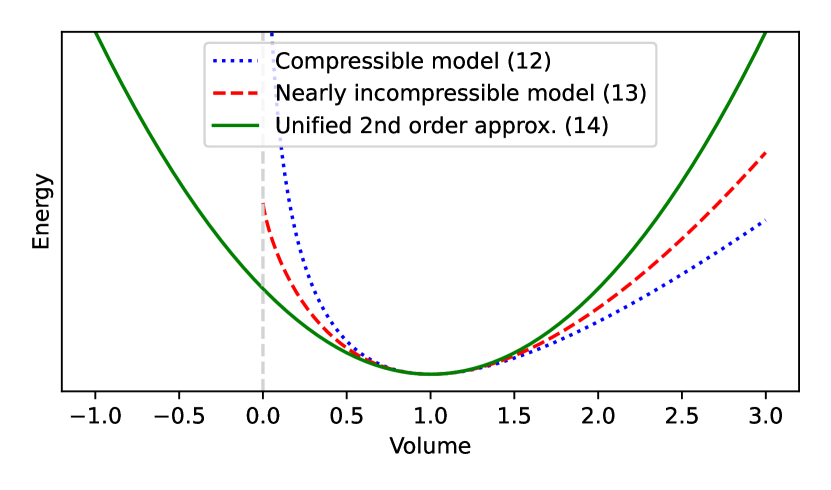
Figure 3. Volume change energy. The energy (negative of work) is plotted for the compressible model in Eq. (18) (dotted curve), the nearly incompressible model in Eq. (19) (dashed curve) and the 2nd order approximate model in Eq. (20) (solid curve). Here $V_{0}=1$ m³, $\kappa_{v}=1$ atm^-1, and $P_{0}=1$ atm. The quadratic model approximates both cases, but is ultimately too weak for excessive compression but too strong during large expansion. Depending on the use case, it may be necessary to model one of Eqs. (18) or (19) directly.

To alleviate the approximation error for scenarios that involve more compression (such as in Figure 9), we recommend decreasing $\kappa_{v}$ to produce stronger restorative forces.

The penalty force is then given directly by the negative derivative of Eq. (20) and controlled by the compression parameter $\kappa_{v}$:

(21) $$\mathbf{f}_{v}(\mathbf{q})=-\frac{(V-V_{0})}{V_{0}\kappa_{v}}\frac{\partial V}{\partial\mathbf{q}}.$$

This can then be added directly to Eq. (2). Incidentally, the Jacobian of Eq. (21) is dense, however, it can be approximated by the sparse term involving $\partial^{2}V/\partial\mathbf{q}^{2}$, which expresses only local force changes. In matrix-free solvers where only matrix-vector products are required, the complete derivative can be computed without hindering performance since the full dense Jacobian is never stored in memory.

4. Numerical Methods

In this section we outline and motivate methods for solving the non-linear force balance system (1).

4.1. Time Integration

The equations of motion (1) can be discretized in time using a variety of implicit time integration methods. Purely explicit integration schemes are not recommended since they prohibitively restrict the admissible time step size in stiff problems — contact and friction can produce extremely large forces causing instability that is intrinsic to the problem we are trying to solve.

Using standard notation, we assume that at time $t$ we know $\boldsymbol{\mathrm{q}}=\boldsymbol{\mathrm{q}}^{t}$ and $\boldsymbol{\mathrm{v}}=\boldsymbol{\mathrm{v}}^{t}$, and employ a step size $h$ to proceed forward in time. The integration methods we consider can be expressed by the momentum balance equation

(22) $$\boldsymbol{\mathrm{0}}=\boldsymbol{\mathrm{r}}(\boldsymbol{\mathrm{v}}^{t+h};h,\boldsymbol{\mathrm{f}},\boldsymbol{\mathrm{M}}),$$

where we use superscripts to indicate time. Each integration scheme is characterized by one or more residual functions $\boldsymbol{\mathrm{r}}$ used to determine the final velocity $\boldsymbol{\mathrm{v}}^{t+h}$. Except for trapezoidal rule, all integrators we consider are L-stable, indicating that they dampen errors for stiff and highly oscillatory or unstable problems. Elastodynamics with frictional contacts can exhibit instabilities (see Section A.2), however, we know that friction is naturally dissipative, and so we expect solutions to behave stably overall. L-stability ensures that any additional stiffness present in the system will not destabilize the numerical solution. For further discussion on stability see (Ascher and Petzold, 1998).

4.1.1. Backward Euler

The simplest implicit scheme is backward Euler (BE), which is typically defined by

(23) $$\boldsymbol{\mathrm{r}}_{\scriptscriptstyle\mathrm{BE}}(\boldsymbol{\mathrm{v}}^{t+h}) =\boldsymbol{\mathrm{M}}(\boldsymbol{\mathrm{v}}^{t+h}-\boldsymbol{\mathrm{v}}^{t})-h\boldsymbol{\mathrm{f}}(\boldsymbol{\mathrm{q}}^{t}+h\boldsymbol{\mathrm{v}}^{t+h},\boldsymbol{\mathrm{v}}^{t+h})=\boldsymbol{\mathrm{0}}.$$

4.1.2. Trapezoidal Rule

A well-known method for mixing explicitly and implicitly determined forces on the system is the trapezoidal rule (TR). We define TR by the momentum balance

$$\boldsymbol{\mathrm{r}}_{\scriptscriptstyle\mathrm{TR}}(\boldsymbol{\mathrm{v}}^{t+h}) =\boldsymbol{\mathrm{M}}(\boldsymbol{\mathrm{v}}^{t+h}-\boldsymbol{\mathrm{v}}^{t})-\frac{h}{2}\left(\boldsymbol{\mathrm{f}}(\boldsymbol{\mathrm{q}}^{t},\boldsymbol{\mathrm{v}}^{t})+\boldsymbol{\mathrm{f}}(\boldsymbol{\mathrm{q}}^{t+h},\boldsymbol{\mathrm{v}}^{t+h})\right)=\boldsymbol{\mathrm{0}},$$

(24) $$\text{where }\boldsymbol{\mathrm{q}}^{t+h} =\boldsymbol{\mathrm{q}}^{t}+\frac{h}{2}\left(\boldsymbol{\mathrm{v}}^{t}+\boldsymbol{\mathrm{v}}^{t+h}\right).$$

Notably, this method is equivalent to the most commonly used implicit Newmark-$\beta$ (Newmark, 1959; Hughes and Knovel, 2000; Géradin et al., 1993) method with $\beta=1/4$ and $\gamma=1/2$. The frictional contact problem we address is not stable, and can generate large stiffnesses for high elastic moduli, large deformations or due to contact and friction. The smoothed frictional contact problem produces high frequency oscillations, which are exacerbated by TR, whereas ideally we want these to be damped away. See Section A.2 for a concrete example. In spite of these flaws, TR is still used in practice, and often decoupled from the frictional contact problem (Li et al., 2020). In Section 5.1.3 we demonstrate how a properly coupled TR as defined in Eq. (24) can resolve some instabilities in practice.

It is also straightforward to use higher-order L-stable methods within our formulation. BDF2, TR-BDF2 and SDIRK2 are defined in the supplemental document, and for further discussion of these methods see (Löschner et al., 2020; Ascher et al., 2022).

4.2. Damped Newton

The momentum balance Eq. (22) can be solved efficiently by second-order root-finding methods like Newton. In the absence of constraints, this can be seen as a generalization of incremental potential optimization (Kane et al., 2000), when the merit function is set to be an energy potential $W(\mathbf{v})$ such that $\partial W(\mathbf{v})/\partial\mathbf{v}=\mathbf{r}(\mathbf{v})$, albeit in that case to maintain a descent direction $\partial\boldsymbol{\mathrm{r}}/\partial\boldsymbol{\mathrm{v}}$ must be appropriately modified to remain positive definite.

Since the presence of friction forces precludes a single potential $W$ for minimization (De Saxcé and Feng, 1998), many methods relying on incremental potentials build special workarounds to solve for exact Coulomb-based friction, including staggered-projections (Kaufman et al., 2008), fixed-point methods (Erleben, 2017) and lagged-friction (Li et al., 2020). Others employ non-smooth Newton to find roots of a proxy function (Bertails-Descoubes et al., 2011; Daviet et al., 2011; Kaufman et al., 2014). Our method is closest to the penalty-based frictional contact approach promoted by Geilinger et al. (2020). We extend this idea by using an implicit sliding basis, which makes our method fully implicit with respect to friction and contact. This unlocks the potential of using larger time steps to get results with good accuracy. For lower resolution examples we use the damped Newton algorithm as defined in Algorithm 1, where the problem Jacobian defined by $\mathbf{J}=\partial\mathbf{r}/\partial\mathbf{v}$ is a square non-symmetric matrix (see Section A.1). Assuming that $\mathbf{J}$ is invertible in the neighborhood of the root, for a sufficiently good initial estimate, damped Newton is guaranteed to converge (Nocedal and Wright, 2006). While singular Jacobians can cause problems, in our experiments they are rare, and often can be eliminated by decreasing the time step in dynamic simulations. Furthermore, in Section A.1 we show that our method does not introduce singularities through coupling between elasticity, contact and friction on a single node.

Input:

$$k_{\text{max}} \leftarrow\text{maximum number of Newton iterations}$$

$$\mathbf{v} \leftarrow\text{previous velocities}$$

Output: $\mathbf{v}_{k}\leftarrow$ velocity for the next time step

1

$\mathbf{v}_{0}\leftarrow\mathbf{v}$

  /* Initialize velocity */

2

3for $k\leftarrow 0$ to $k_{\text{max}}$ do

4       if ShouldStop$(\mathbf{r}(\mathbf{v}_{k}),\mathbf{v}_{k})$ then

5             break

6            

7       end if

      $\mathbf{p}_{k}\leftarrow-\mathbf{J}(\mathbf{v}_{k})^{-1}\mathbf{r}(\mathbf{v}_{k})$

        /* Set search direction */

8      

9      $\alpha\leftarrow\text{\sc LineSearch}(\mathbf{v}_{k},\mathbf{p}_{k})$

10       $\mathbf{v}_{k+1}\leftarrow\mathbf{v}_{k}+\alpha\mathbf{p}_{k}$

11      

12 end for

ALGORITHM 1 DampedNewton

4.3. Inexact Damped Newton

For large scale problems, it is often preferable to use an iterative linear solver, which can outperform a direct solver when degrees of freedom are sufficiently abundant. We use inexact Newton to closely couple the iterative solver with our damped Newton’s method.

Since friction forces produce a non-symmetric Jacobian, we chose the biconjugate gradient stabilized (BiCGSTAB) algorithm (van der Vorst, 1992) to find Newton search directions $\boldsymbol{\mathrm{p}}_{k}$. For Jacobian $\boldsymbol{\mathrm{J}}_{k}=\partial\boldsymbol{\mathrm{r}}_{k}/\partial\boldsymbol{\mathrm{v}}$ with $\boldsymbol{\mathrm{r}}_{k}=\boldsymbol{\mathrm{r}}(\boldsymbol{\mathrm{v}}_{k})$, the search direction is determined by

$$\left\|\boldsymbol{\mathrm{r}}_{k}+\boldsymbol{\mathrm{J}}_{k}\boldsymbol{\mathrm{p}}_{k}\right\|\leq\sigma_{k}\|\boldsymbol{\mathrm{r}}_{k}\|,$$

where $\sigma_{k}=\min(\|\boldsymbol{\mathrm{r}}_{k}\|^{\varphi}/\|\boldsymbol{\mathrm{r}}_{k-1}\|^{\varphi},\sigma)$ and $\varphi=(1+\sqrt{5})/2$ to maintain Q-quadratic convergence (Eisenstat and Walker, 1996).

Using BiCGSTAB as the iterative solver additionally allows one to use forward automatic differentiation to efficiently compute products $\mathbf{J}\mathbf{p}$.

The final inexact Newton algorithm is presented in Algorithm 2.

Input:

$$k_{\text{max}} \leftarrow\text{maximum number of Newton iterations}$$

$$\mathbf{v} \leftarrow\text{previous velocities}$$

$$c_{1} \leftarrow 10^{-4}$$

Output: $\mathbf{v}_{k}\leftarrow$ velocity for the next time step

1

$\mathbf{v}_{0}\leftarrow\mathbf{v}$

  /* Initialize velocity */

2

3for $k\leftarrow 0$ to $k_{\text{max}}$ do

4       if ShouldStop$(\mathbf{r}(\mathbf{v}_{k}),\mathbf{v}_{k})$ then

5             break

6            

7       end if

8      $\sigma_{k}\leftarrow\min(\|\boldsymbol{\mathrm{r}}_{k}\|^{\varphi}/\|r_{k-1}\|^{\varphi},\sigma)$

9       Find $\mathbf{p}_{k}$ such that $\left\|\boldsymbol{\mathrm{r}}_{k}+\boldsymbol{\mathrm{J}}_{k}\boldsymbol{\mathrm{p}}_{k}\right\|\leq\sigma_{k}\|\boldsymbol{\mathrm{r}}_{k}\|$

10      

11      $\alpha\leftarrow 1$

      

       /* Backtracking */

12       while $\|\mathbf{r}(\mathbf{v}+\alpha\mathbf{p})\|>(1-c_{1}\alpha(1-\sigma_{k}))\|\mathbf{r}(\mathbf{v}_{k})\|$ do

13             $\alpha\leftarrow\rho\alpha$

14            

15       end while

16      $\sigma_{k}\leftarrow 1-\alpha(1-\sigma_{k})$

17       $\mathbf{v}_{k+1}\leftarrow\mathbf{v}_{k}+\alpha\mathbf{p}_{k}$

18      

19 end for

ALGORITHM 2 InexactDampedNewton

4.4. Contact

To ensure that no penetrations remain (i.e. $d_{i}>0$ for each contact $i$) at the end of the time step we measure the deepest penetration depth $d_{\text{deepest}}=\min_{i}(\boldsymbol{\mathrm{d}}_{i}(\boldsymbol{\mathrm{q}}^{t+h}))$, and bump the contact stiffness parameter $\kappa$ by the factor $\frac{b^{\prime}(d_{\text{deepest}})}{b^{\prime}(0.5\delta)}$ whenever $d_{\text{deepest}}<0$, where $b^{\prime}$ is the scalar derivative of $b$. The same step is then repeated with the new $\kappa$. This scheme sets the optimal contact penalty value found by the Newton scheme to appear for contacts $0.5\delta$ outside the contact surface. As such, in most cases one time step with an additional contact iteration is sufficient before all contacts are resolved. Furthermore, $\kappa$ is never decreased so long as there are active contacts to avoid oscillations at the contact surface.

The downside of this technique is that it compromises the smoothness of the simulation. We postulate that in practice, this may not be problematic in a differentiable pipeline since $\kappa$ is not changed frequently and subsequent differentiable iterations can carry forward the maximal $\kappa$ to maintain smoothness.

4.5. Compatibility with IPC

Li et al. (2020) introduced a robust method to resolve contacts by minimizing incremental potentials with friction being evaluated using lagged positional estimates from the previous time step. Here we express the IPC method as a nonlinear system, and propose a simple change that will establish accurate frictional responses. The total force with lagged friction can be expressed as

(25) $$\mathbf{f}_{\mathit{lag}}(\mathbf{q}^{t},\mathbf{q}^{t+h},\mathbf{v}^{t+h})=\mathbf{f}_{\mathit{edcg}}(\mathbf{q}^{t+h},\mathbf{v}^{t+h})+\mathbf{f}_{f}(\mathbf{q}^{t},\mathbf{v}^{t+h}),$$

where $\mathbf{f}_{\mathit{edcg}}$ is the sum of elastic, damping, contact and external forces and $\mathbf{f}_{f}$ is the friction force as before. This net force can then be integrated with an implicit-explicit (IMEX) style scheme. Specifically for BE and TR we get

(26) $$\mathbf{r}_{\text{BE,IPC}}(\mathbf{v}^{t+h}) =\mathbf{v}^{t+h}-\mathbf{v}^{t}-h\mathbf{M}^{-1}\mathbf{f}_{\mathit{lag}}(\mathbf{q}^{t},\mathbf{q}^{t+h},\mathbf{v}^{t+h}),$$

$$\mathbf{r}_{\text{TR,IPC}}(\mathbf{v}^{t+h}) =\mathbf{v}^{t+h}-\mathbf{v}^{t}$$

(27) $$-\frac{h}{2}\mathbf{M}^{-1} \left(\mathbf{f}_{\mathit{lag}}(\mathbf{q}^{t},\mathbf{q}^{t+h},\mathbf{v}^{t+h})+\mathbf{f}_{\mathit{lag}}(\mathbf{q}^{t},\mathbf{q}^{t},\mathbf{v}^{t})\right),$$

respectively. This formulation has the advantage of having a well-defined antiderivative with respect to $\mathbf{v}^{t+h}$, which can be minimized using common optimization tools. In this view, IPC effectively solves Eqs. (26) or (27) using the proposed log-barrier potential as a merit function, CCD aided line search and Hessian projection. Although this can be done iteratively with better estimates for the lagged friction force, this approach has limitations as demonstrated in Section 5.1.1. Instead, we can establish accurate friction in IPC, if we abandon the popular optimization view and instead solve the original momentum balance problem where friction forces are resolved implicitly (e.g. replace $\boldsymbol{\mathrm{f}}_{f}(\boldsymbol{\mathrm{q}}^{t},\boldsymbol{\mathrm{v}}^{t+h})$ with $\boldsymbol{\mathrm{f}}_{f}(\boldsymbol{\mathrm{q}}^{t+h},\boldsymbol{\mathrm{v}}^{t+h})$ for BE).

5. Results

All examples were run on the AMD Ryzen Threadripper 1920X CPU with 12 cores, 24 threads at 3.7 GHz boost clock and 32 GB RAM. We used Blender 3.1 (2021) for all 3D renderings. For Algorithm 1 we used the Intel MKL sparse LU solver to solve the square non-symmetric linear system on line 1. We used dual numbers for forward automatic differentiation (Larionov, 2022) and a custom BiCGSTAB implementation for the inexact Newton Algorithm 2. In the following results Algorithms 1 and 2 are dubbed “Direct” and “Iterative”, respectively, since the former uses a direct linear solver and the latter uses an iterative linear solver.

5.1. Friction accuracy

With the following examples we demonstrate two scenarios where lagged friction causes large deviations from an expected accurate and stable friction response.

5.1.1. Block slide

In this example we let a stiff elastic block slide down a 10 degree slope expecting it to stop for $\mu=0.177>\tan(10^{\circ})$ after sliding for a total of $x_{T}=0.769$ m for $T=15.38$ seconds (see supplemental document for details on the experiment).

In Figure 4 we demonstrate that our method produces consistent stopping across a variety of time step sizes using BE and TR time integration. We compare against a state-of-the-art smoothed friction method (Li et al., 2020) using a lagged friction approach to show that it fails to establish consistent stopping with BE, and fails to stop with TR altogether after 50 seconds. We reproduce the lagged friction method in our simulator to demonstrate that TR can be used to generate reliable stopping if the equations of motion are correctly integrated as in Eq. (27). Our method produces a more accurate stopping distance using TR than IPC does using BE even after using multiple fixed point iterations.

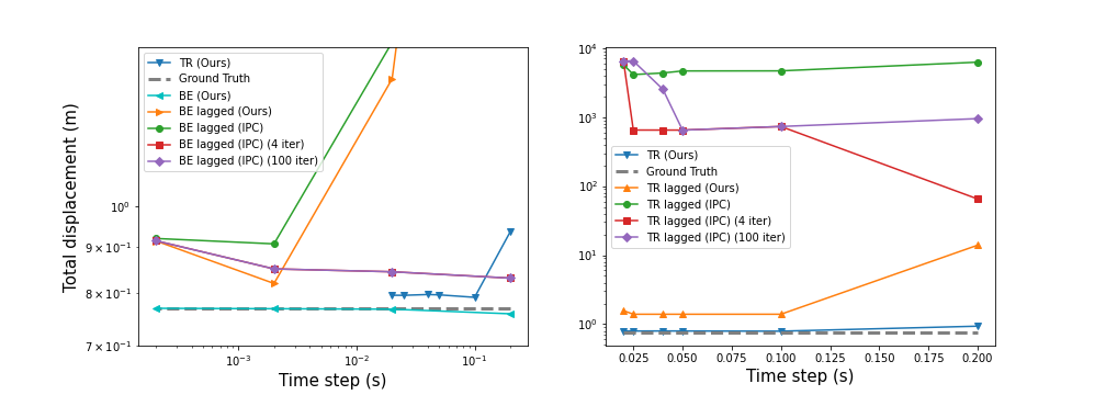
(a) Total displacement travelled by the block before coming to a stop. With BE and multiple fixed point iterations the lagged friction approach can produce a reasonable approximation of the stopping behavior, however, the approximation does not converge to the true solution. Our method produces an accurate estimate of the true behavior with BE, while TR produces a better estimate than lagged friction at $h=0.1$ s and lower. With lagged friction, the TR method presented in Eq. (27) produces a more accurate result than IPC since contact is handled together with other implicit forces.

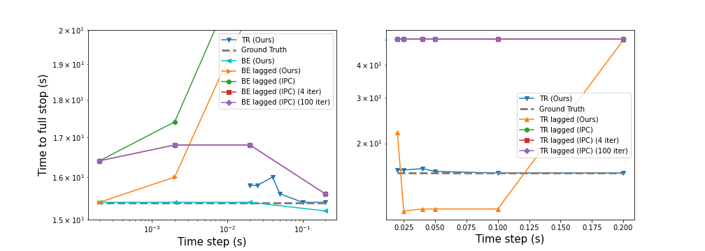
(b) Time taken by each block to come to a stop. With BE, our method produces an accurate approximation to the true stopping time for all but the largest time step. In contrast, lagged friction fails to converge to the true stopping time under multiple fixed point iterations. With TR, the approximation is not as accurate as with BE, although still closer to the true value than lagged friction using BE. With TR, lagged friction does not produce a reliable stopping time, even under refinement. Using IPC’s TR implementation, the box does not stop after 50 s for any time step.

Figure 4. Block slide. Comparisons of analytic stopping conditions of a sliding block to numerical results.

5.1.2. Bowl grasp

Control over the friction coefficient is particularly important in grasping scenarios since grasped objects are often delicate. This means that friction forces involved in lifting are often close to the sliding threshold.

As shown in Figure 1, an upside down bowl is lifted using 3 soft pads to compare sticking stability of lagged friction proposed in Eq. (26) against a fully implicit method from Eq. (23). The bowl is successfully picked up and stuck to the pads for a range of time steps when using the implicit method, however it slips for different time step values with lagged friction. The height of the bowl is plotted in Figure 5 for each method and time step combination.

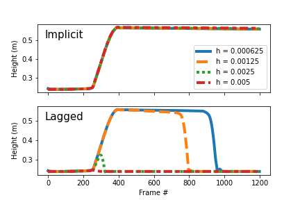
Figure 5. The height of the bowl in Figure 1 is plotted against frame number time step $h$ is varied. Here the bowl slips for the lagged friction method, whereas the fully implicit method maintains stable sticking for every time step, hence all plotted lines overlap.

5.1.3. Ball in a box

A rubber ball placed inside an elastic box has an initial spin of 4800 rotations per minute and an initial velocity set to $\vec{v}_{0}=(-0.923,-0.385,0)$. In Figure 6, we demonstrate how our fully coupled TR integrator produces more stable dynamic simulations when compared to the decoupled TR as proposed by Li et al. (2020). This scenario is simulated with both methods for 800 frames at $h=0.01$ s with comparable damping parameters as shown in Figure 6(b). The TR implementation used by IPC blows up, whereas in our formulation the energy is eventually dissipated as expected.

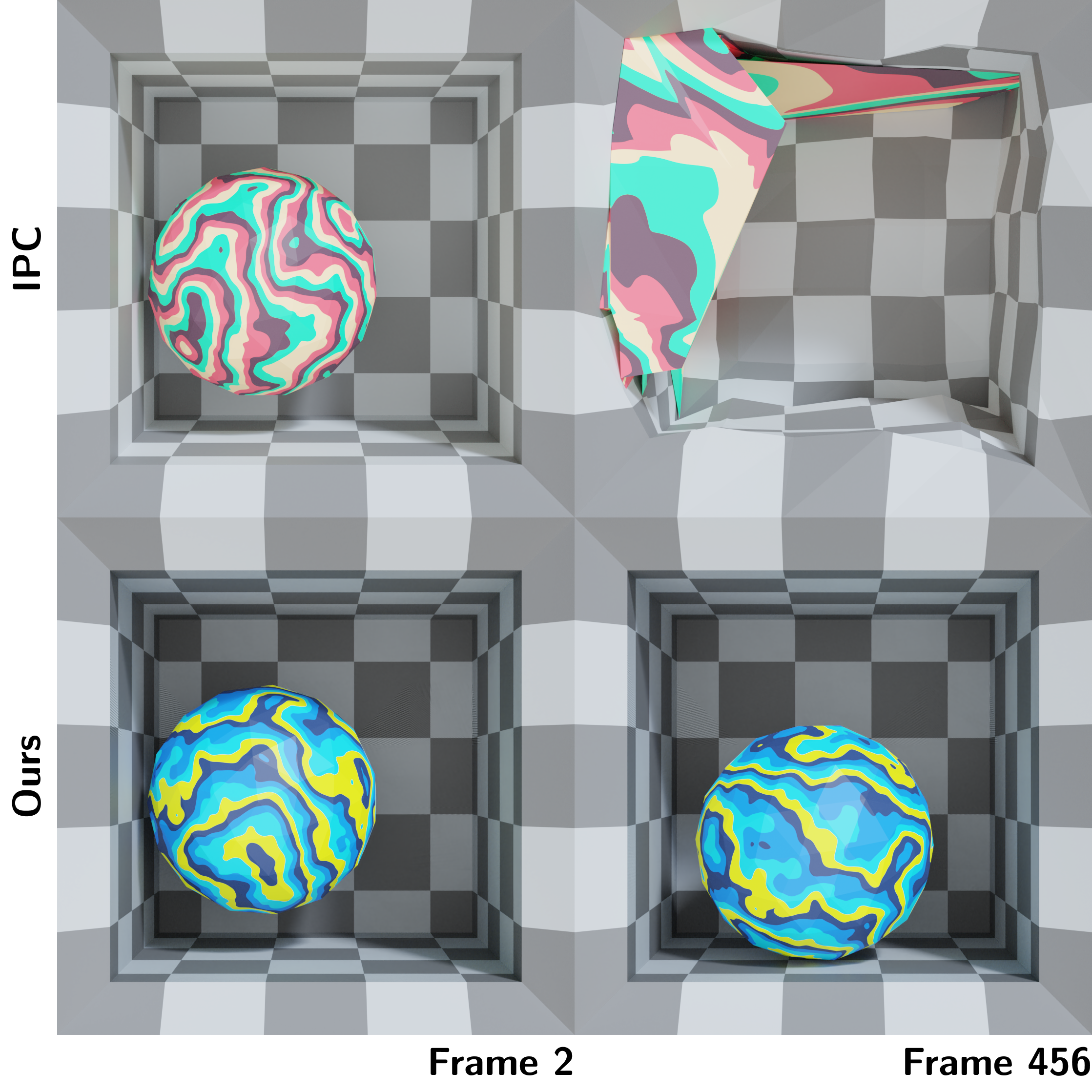
(a) The TR formulation proposed in IPC is unstable (top row) whereas our method produces a dissipative scenario (bottom row) even with a slightly weaker damping as shown in Figure 6(b).

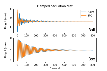
(b) Damping ratio of 0.02 is selected for IPC, and damping parameter of 0.1 Hz is set for our model. In both cases Rayleigh damping is used. The ball (top) and the box (bottom) are simulated individually with both methods and centroid heights are plotted to ensure the that oscillation amplitudes with TR as implemented by IPC do not exceed those generated by our implementation. This test ensures that the reason for blowup in IPC is not due to integration of elasticity equations alone, but indeed due to loose coupling between elastic and contact terms.

Figure 6. Ball in a box. A spinning ball bounces inside an elastic box. Here $\rho=10000$ kg/m³, $E=500$ KPa, and $\nu=0.1$ for the box and $\rho=500$ kg/m³, $E=50$ KPa and $\nu=0.45$ for the ball, with friction coefficient set to $\mu=0.1$ between them.

5.2. Performance

In this section, we show how various combinations of volume preservation and frictional contact constraints can affect the performance of the simulation. In addition, we compare Algorithms 1 and 2 in performance and memory usage.

5.2.1. Tube cloth bend

The inexact Newton Algorithm 2 shines particularly in scenarios with numerous contacts, such as with tight-fitting garments, where the entire garment is in contact with a body. Here we simulate a simplified scenario of a tube cloth wrapped around a bending soft object resembling an elbow or knee as depicted in Figure 7. Table 1 shows the corresponding timing results, which indicate that inexact Newton performs much better than the damped Newton algorithm employing a direct solver. Furthermore, the performance gap becomes large when the number of elements is increased. Interestingly this data also indicates that larger friction coefficients cause a bigger bottleneck for the solve compared even to stiff volume change penalties (indicated by small $\kappa_{v}$).

\begin{overpic}[width=143.09538pt,trim=281.04999pt 0.0pt 401.49998pt 0.0pt,clip]{img/bend/lores_1.png} \put(5.0,17.0){3K Triangles} \put(5.0,5.0){5K Tetrahedra} \end{overpic}

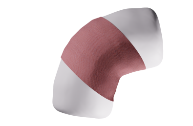
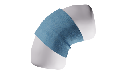
\begin{overpic}[width=143.09538pt,trim=281.04999pt 0.0pt 401.49998pt 0.0pt,clip]{img/bend/hires_1.png} \put(5.0,17.0){8K Triangles} \put(5.0,5.0){30K Tetrahedra} \end{overpic}

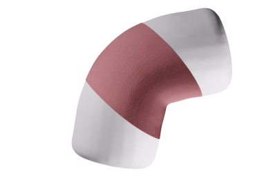
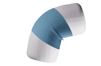
Figure 7. Tube cloth bend. A cylindrical garment is wrapped around a bending capsule. Lower resolution example is shown at the top row and higher resolution at the bottom row. The first column shows the initial configuration, second column shows the end result with low friction ($\mu=0.2$), and the last column shows the end result with high friction ($\mu=0.8$).

# Elements	$\mu$	Solver Type	$\kappa_{v}$	Time	Memory	Volume Loss
3K Tris 5K Tets	0.2	Iterative	-	4.81	1.84 GB	0.962%
		Direct	-	22.1	6.51 GB	0.962%
	0.8	Iterative	-	12.7	1.91 GB	0.962%
		Direct	-	25.6	7.09 GB	0.962%
8K Tris 30K Tets	0.2	Iterative	-	8.59	830 MB	2.55%
		Iterative	4.6e-5	12.2	858 MB	2.44e-4%
	0.8	Iterative	-	51.6	625 MB	2.57%
		Iterative	4.6e-5	53.2	918 MB	2.44e-4%

Table 1. Tube cloth bend performance data. Time is measured in seconds per frame and memory refers to total memory growth during the simulation as reported by Houdini’s performance monitor. Simulations without volume change penalty have $\kappa_{v}$ set to $-$.

5.2.2. Ball Squish

A hollow ball at various resolutions (1K, 55K and 160K elements) is pressed between two flat planes as demonstrated in Figure 8. As a result the ball experiences volume loss. To preserve some of the volume we simulate the compression with compression coefficients $\kappa_{v}=1$ (e.g. a ball filled with air) and $\kappa_{v}=0.01$ (e.g. a ball filled with water). In the latter case we expect significantly less volume loss, which is reflected in our experiments as shown in Table 2. Furthermore, we note from Table 2(b) that scenarios with small $\kappa_{v}$ favor the “Iterative” method. In Table 2(c) we see that this is true whether $\mathbf{J}$ is sparsely approximated (“Inexact”) or not (“Exact”). In contrast, stiffer scenarios prefer the “Direct” method due to worse system conditioning.

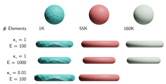
Figure 8. Ball squish. A hollow ball of various resolutions is squished between two parallel rigid plates. The same simulations is performed for varying Young’s moduli $E$ and compression coefficients $\kappa_{v}$.

# Elements	1K	55K	160K
Direct	0.354 (0.228)	15.9 (1.69)	61.0 (4.26)
Iterative	0.391 (0.081)	31.9 (0.719)	111 (1.92)
Volume loss	33.6%	27.8%	27.7%

(a) $E=100$ KPa, $\kappa_{v}=1$.

# Elements	1K	55K
Direct	1.08 (0.478)	89.1 (2.03)
Iterative	0.463 (0.214)	42.6 (0.884)
Volume loss	0.49%	0.36%

(b) $E=100$ KPa, $\kappa_{v}=0.01$.

$\kappa_{v}=$	1	0.01
Direct Exact $\mathbf{J}$	0.832 (0.393)	0.871 (0.672)
Direct Inexact $\mathbf{J}$	0.354 (0.228)	1.08 (0.478)
Iterative	0.391 (0.081)	0.463 (0.214)

(c) $E=100$ KPa, for 1K elements.

# Elements	1K	55K	160K
Direct	0.312 (0.388)	8.28 (1.52)	25.5 (4.14)
Iterative	0.593 (0.097)	28.3 (0.732)	56.2 (2.62)
Volume loss	74.3%	74.6%	75.0%

(d) $E=1000$ KPa with no volume preservation constraint.

Table 2. Ball squish timings, memory usage and volume loss. A hollow ball is squished between two flat rigid plates at time step $h=0.001$ s. Timings are given in seconds per frame and averaged over 804 frames. The memory usage measured in GB over the entire simulation sequence is shown in parentheses. Volume loss is computed as the change in volume between frames 1 and 804 as a percentage of initial volume inside the ball. Each table specifies the number of elements, Young’s modulus $E$ and compression coefficient $\kappa_{v}$ where applicable. Here we compare how the performance characteristics of our “Direct” and “Iterative” methods change when problem stiffness and $\kappa_{v}$ is varied for different mesh resolutions.

5.3. Real world phenomena

In the following example we show how our simulator can reproduce deformations captured in the real world.

5.3.1. Tennis ball

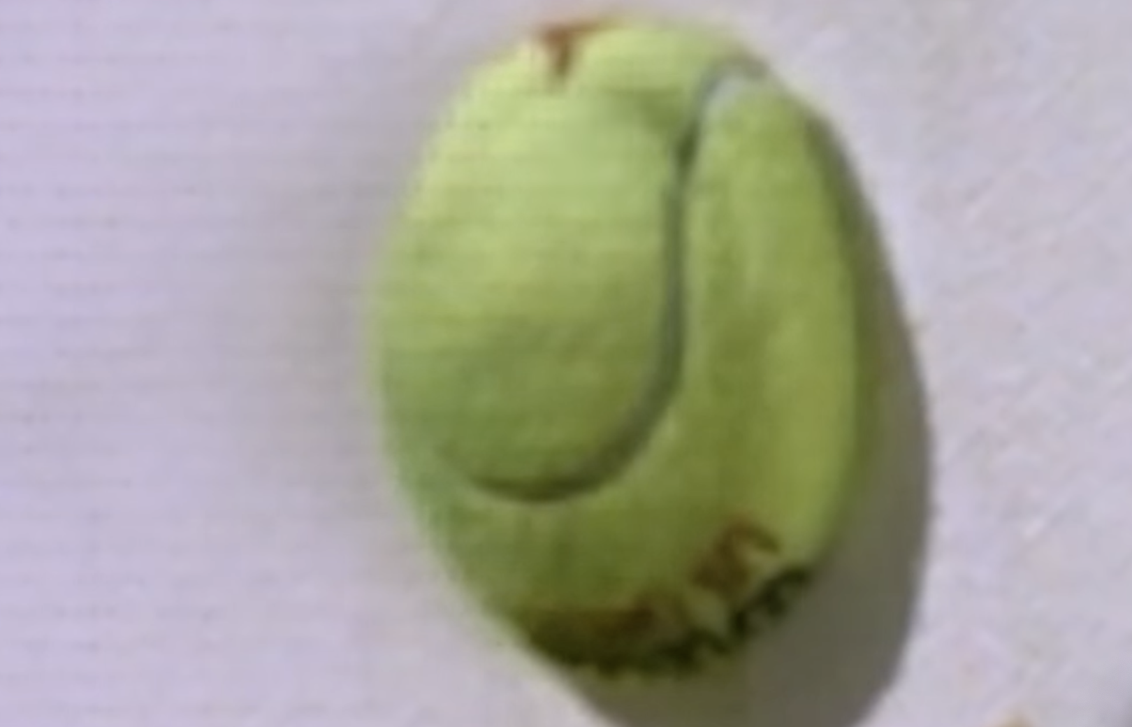
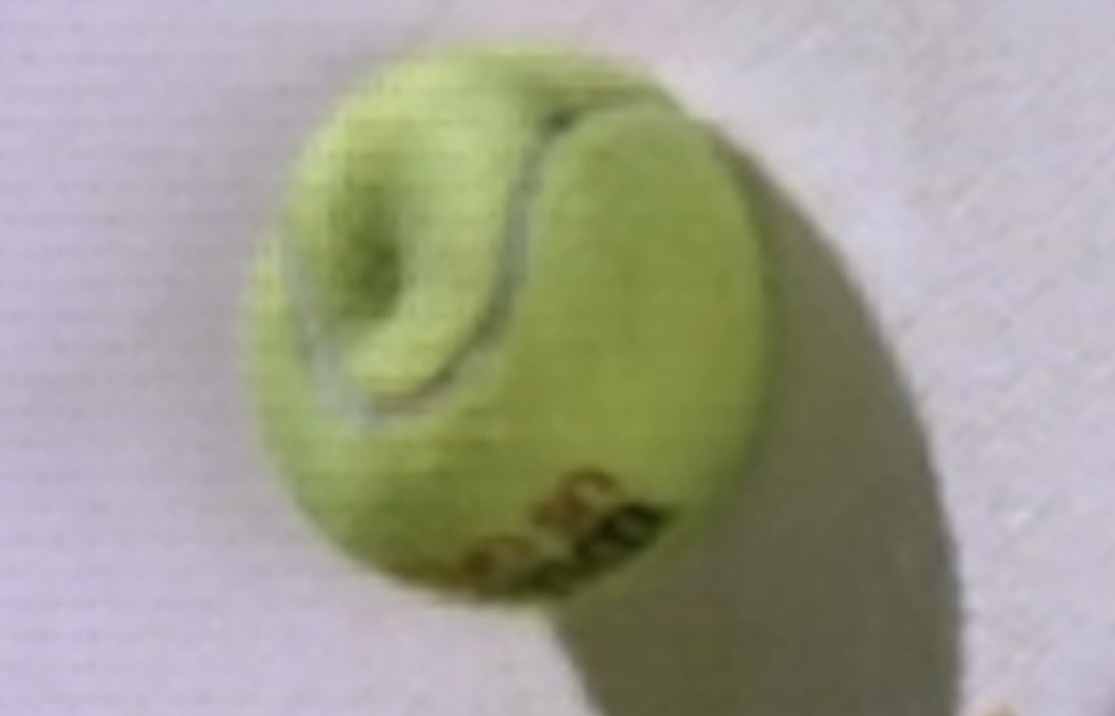
Figure 9. Highspeed tennis ball collision. Simulated hollow tennis ball collides against a wall at 100mph. The deformation here closely resembles that of a real tennis ball as captured by Anderson (2018).

Tennis ball dynamics is a prime example of all methods proposed in this paper. We launch a tennis ball at a wall at 100 mph (44.7 m/s) to reproduce accurate slow motion deformation. Tennis balls are typically pressurized to approximately 1 atm above atmospheric pressure to increase longevity and to produce a livelier bounce during play. In Figure 9 we show how deformation changes when the ball is pressurized and compare the result with live footage. The simulation contains 100K tetrahedra and 92K vertices. The ball is hollow with a stiff inner core ($E=6$ MPa, $\nu=0.4995$ and $\rho=934$ kg/m³) and a light outer felt material ($E=5.4$ MPa, $\nu=0.3$ and $\rho=4.69$ kg/m³). The volume change penalty is applied to the interior of the ball. This 1000 frame simulation took 4.89 seconds per frame and a total of 11.33 GB in memory.

Next, a tennis ball is dropped from a 254 cm height to evaluate its bounce with and without pressurization. We show how pressurization and choice of integrator can drastically affect the height of the bounce in Figure 10.

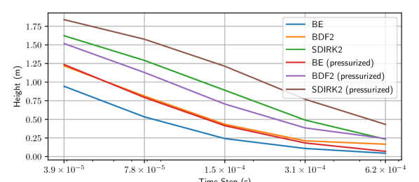
Figure 10. Tennis ball drop. A pressurized and non-pressurized tennis ball dropped from a 254 cm height, is simulated using different integrators. The pressurized ball bounces higher than the corresponding non-pressurized ball as expected for each integrator. BE and BDF2 produce a much lower bounce than SDIRK2 across a range of different time steps highlighting the significance of higher-order integration in this test. Higher-order integrators are defined in the supplemental document.

5.3.2. Tire wrinkling

We model an inflated tire used by top fuel dragsters to show the folding phenomenon at the start of the race. The tires are deliberately inflated at a low pressure of 0.68 atm above atmospheric pressure, which allows them to better grip the asphalt for a better head start. As a result the soft tire tends to wrinkle as the wheels start to turn. This phenomenon allows for a larger contact patch between the tire and the ground for better traction, which translates to a larger acceleration. In Figure 11 we demonstrate this phenomenon in simulation with a shell model tire inflated using our volume change penalty. The outer side of the tire is initially stuck to the ground and then dragged while maintaining consistent contact. Accurate simulation of stick-slip transitions of the tire is critical in determining its performance since traction transfers torque into forward acceleration of the vehicle, which ultimately determines the outcome of a race. The tire is simulated using 18K triangles and 9K vertices. The tire mesh is split into an outer stiffer part that is in contact with the ground and a softer inner part where the label is printed. Here $\mu=0.8$, and $\nu=0.49$ everywhere, while $E=400$ KN/m, $\rho=200$ kg/m² and bending stiffness set at $0.1$ on the outer part, and $E=200$ KN/m, $\rho=50$ kg/m², and bending stiffness set at $0.01$ on the inner part. The simulation ran with $h=0.00125$ s for $3.63$ seconds per frame using the damped Newton solver.

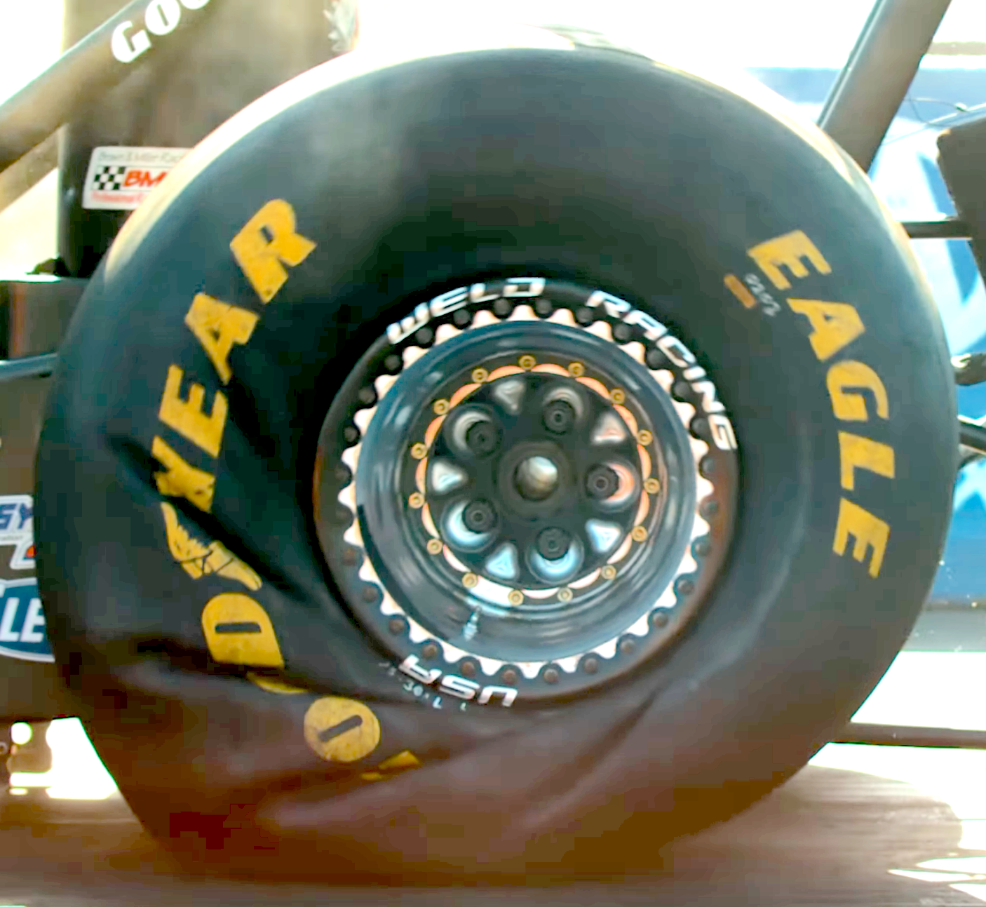
Figure 11. Dragster tire wrinkle. A soft tire spins against the ground with a large friction coefficient, causing the rubber to wrinkle. Left: simulation of the tire being rotated in place causing the wrinkle due to a high coefficient of friction ($\mu=0.8$) with the ground. Right: a real dragster tire exhibiting the wrinkle phenomenon at the start of the race (Goodyear, 2020).

6. Conclusions and Limitations

Smooth contact

An important detail of our formulation is that it requires a smooth contact surface representation in order to guarantee local convergence of Newton’s method. This also implies that for each step the collision detection algorithm must capture all potential collisions within distance $\delta$. Otherwise, a collision detected after it has become closer than $\delta$ away from the contact surface will cause a discontinuity in contact forces. This may occasionally cause oscillations in Newton’s iterations if the root lies near the discontinuity.

Local minima

Solving for roots of nonlinear momentum equations allows one to resolve friction forces accurately, however, this comes with a trade-off. Optimization theory allows one to reliably find a descent direction even when the objective Hessian is indefinite via projection or filtering techniques. Although computing the descent direction for finding roots of nonlinear equations allows one to use the entire unfiltered Jacobian, global convergence can only be theoretically guaranteed when the Jacobian is bounded on the neighborhood of the initial point. For stiff systems, this assumption can become problematic, although the practical implications are unclear.

Hydrostatic equilibrium

Our volume change penalty model expects hydrostatic equilibrium, which may not always be a good approximation given the rate of change of volume during a simulation. For quickly deforming objects like in our tennis ball and tire wrinkling example, some details of the deformation may be missing due to this approximation. This is because the object deforms faster than the air moves inside the volume, creating non-uniform pressure distribution throughout the volume. The comparison of our hydrostatic model to a fully dynamic fluid simulation remains as future work.

In conclusion, we presented a fully implicit method for simulating hyperelastic objects subject to frictional contacts. This method generalizes the popular optimization framework for simulating hyperelastics with contact and lagged friction potentials. We demonstrate how integrators like trapezoid rule or higher order integrators can be applied in our method as well as in IPC-style frameworks. Our method addresses the lack of friction convergence in lagged friction formulations by evaluating contacts, friction forces as well as tangential bases implicitly.

Furthermore, we propose a physically-based volume change penalty that can be used to simulate compressible as well as nearly incompressible solids in a single framework without additional complex constraint solvers.

Our system is entirely smooth, featuring unique gradients, which are ideal for differentiable simulation.

Appendix A 2D Analysis

To simplify our analysis and better illustrate the problem, consider a simple 2D example. A mass is attached by an idealized spring to the origin resting on a conveyor belt, which moves left at a constant velocity as illustrated in Figure 12.

Figure 12. Springy rod example in 2D. A rod with spring constant $k$ is fixed at the top (filled circle) and rests on the belt with the free end (hollow circle) experiencing a contact force $\boldsymbol{\mathrm{f}}_{c}$. The belt moves to the left at a constant velocity $\boldsymbol{\mathrm{v}}_{s}$ causing a friction force $\boldsymbol{\mathrm{f}}_{f}$ on the free end of the rod.

Using this example we analytically evaluate the conditioning of single point frictional contacts, and demonstrate potential issues that can arise in the formulation.

We evaluate our methods on the simple 2D example proposed in Section 1. We developed the following 2D simulations in the Julia programming language (Bezanson et al., 2012) using Jupyter notebooks. The 2D equations of motion (1) for this problem can be written as

$$\boldsymbol{\mathrm{M}}\dot{\boldsymbol{\mathrm{v}}}=\boldsymbol{\mathrm{K}}\boldsymbol{\mathrm{q}}-\boldsymbol{\mathrm{D}}\boldsymbol{\mathrm{v}}+\mu b^{\prime}(q_{y})\boldsymbol{\mathrm{\eta}}(\boldsymbol{\mathrm{v}}-\boldsymbol{\mathrm{v}}_{s})+\boldsymbol{\mathrm{f}}_{c}+\boldsymbol{\mathrm{M}}\boldsymbol{\mathrm{g}},$$

where $\boldsymbol{\mathrm{q}}$ and $\boldsymbol{\mathrm{v}}$ are the 2D position and velocity of the free end respectively, $\boldsymbol{\mathrm{K}}=-k(l_{0}-\|\boldsymbol{\mathrm{q}}\|)/\|\boldsymbol{\mathrm{q}}\|$, $l_{0}$ is the rest length of the spring, $\boldsymbol{\mathrm{f}}_{c}=(0,-b^{\prime}(q_{y}))^{\top}$ and $\boldsymbol{\mathrm{g}}$ is gravitational acceleration.

In this case the gap function is simplified to $\boldsymbol{\mathrm{d}}(\boldsymbol{\mathrm{q}})=(0,q_{y})$, and $\boldsymbol{\mathrm{T}}$ is the projection onto the $x$-axis.

A.1. Jacobian conditioning

First we demonstrate the asymmetry of $\boldsymbol{\mathrm{J}}$ for this problem to illustrate why we need solvers for non-symmetric linear systems. Here we will investigate backward Euler, however, the same findings should also apply for other integrators.

When the contact is not activated (i.e. $q_{y}\geq\delta$ in the 2D problem), both friction and contact forces are zero, reducing the problem to damped elastodynamics. In this case it is well known that $\boldsymbol{\mathrm{J}}$ is symmetric and often even positive definite, a thorough eigenanalysis of this case is explored by Smith et al. (2018).

For the activated case (i.e. $q_{y}<\delta$), we will use Eq. (15) to analyze the 2D example. It models sticking, pre-sliding and sliding stages of friction with a single smooth function.

The derivative of Eq. (23) for our 2D problem is a $2\times 2$ matrix

$$\boldsymbol{\mathrm{J}}_{\scriptscriptstyle\mathrm{BE}}=\boldsymbol{\mathrm{J}}_{\scriptscriptstyle\mathrm{BE}}^{\text{inactive}}+\begin{bmatrix}J_{xx}&J_{xy}\\ J_{yx}&J_{yy}\end{bmatrix},$$

where $\boldsymbol{\mathrm{J}}_{\scriptscriptstyle\mathrm{BE}}^{\text{inactive}}$ identifies the part without friction or contact. When the contact is not active, we simply have $\boldsymbol{\mathrm{J}}_{\scriptscriptstyle\mathrm{BE}}=\boldsymbol{\mathrm{J}}_{\scriptscriptstyle\mathrm{BE}}^{\text{inactive}}$. For active contacts, we have

$$J_{xx} =-J_{yy}\frac{\mu\epsilon(q_{y}-\delta+1)}{2h(\epsilon+|v_{s}|)^{2}}, J_{xy} =J_{yy}\frac{\mu v_{s}}{\epsilon+|v_{s}|},$$

$$J_{yx} =0, J_{yy} =-\frac{6h^{2}\kappa}{m\delta}(q_{y}-\delta+1),$$

assuming that the velocity at the free end is zero. Here $m$ is the mass of the free end. Other quantities are as defined in previous sections. These expressions demonstrate a couple of interesting properties of frictional contact:

• Asymmetry of the Jacobian is due only to friction. Frictionless contact ($\mu=0$) produces a symmetric system. Optimization based methods (Li et al., 2020; Larionov et al., 2021) work around this asymmetry using time splitting or explicit integration, where friction is solved separately from the main elasticity equations. This is problematic because friction, contact and elasticity produce comparable impulses for large time steps, especially for large elastic moduli.

• When $v_{s}$ vanishes (i.e. sticking), $J_{xx}$ becomes very sensitive to the stick-slip parameter $\epsilon$, which suggests potentially poor conditioning.

We can symbolically compute the singular values of $\boldsymbol{\mathrm{J}}_{\scriptscriptstyle\mathrm{BE}}$ to evaluate how the conditioning of this matrix depends on $h$, $\kappa$, $\delta$, and $\epsilon$ parameters. As mentioned before we are especially interested in the case where $v_{s}=0$, the sticking case, where conditioning is poor. The following properties can be computed symbolically:

(28) $$\lim_{\kappa\to\infty}\mathrm{cond}(\boldsymbol{\mathrm{J}}_{\scriptscriptstyle\mathrm{BE}}) =\max\left(\frac{2h\epsilon}{\delta\mu},\frac{\delta\mu}{2h\epsilon}\right)$$

(29) $$\mathrm{cond}(\boldsymbol{\mathrm{J}}_{\scriptscriptstyle\mathrm{BE}}) \in O(\min(\tfrac{1}{\delta},\kappa)) \text{ as }\delta\to 0\text{ and }\kappa\to\infty$$

(30) $$\mathrm{cond}(\boldsymbol{\mathrm{J}}_{\scriptscriptstyle\mathrm{BE}}) \in O(\tfrac{1}{\epsilon}) \text{ as }\epsilon\to 0$$

In consequence, we know that:

1. For arbitrarily large $\kappa$, the conditioning of $\boldsymbol{\mathrm{J}}_{\scriptscriptstyle\mathrm{BE}}$ is bounded above by a function of $\delta$ by Eq. (28).

2. Conditioning will not degrade further when $\kappa$ is increased if $\kappa>1/\delta$ by Eq. (29).

3. $\mathrm{cond}(\boldsymbol{\mathrm{J}}_{\scriptscriptstyle\mathrm{BE}})$ can grow linearly with $1/\epsilon$ by Eq. (30).

This analysis further expands on the tradeoffs introduced by the smoothed friction formulation. We can use these relationships to pick appropriate values of $\epsilon$ and $\delta$ for a particular application.

A.2. Stability

Our 2D problem can exhibit instabilities, two of which we will address here.

We can rewrite the balance equation (1) with $\boldsymbol{\mathrm{v}}=\dot{\boldsymbol{\mathrm{q}}}$ as a single system where $\boldsymbol{\mathrm{u}}=(\boldsymbol{\mathrm{q}},\boldsymbol{\mathrm{v}})^{\top}$ and

$$\dot{\boldsymbol{\mathrm{u}}}=\boldsymbol{\mathrm{F}}(\boldsymbol{\mathrm{u}})=\begin{bmatrix}\boldsymbol{\mathrm{v}}\\ \boldsymbol{\mathrm{f}}(\boldsymbol{\mathrm{q}},\boldsymbol{\mathrm{v}})\end{bmatrix}.$$

Although $\boldsymbol{\mathrm{F}}$ is non-linear, we can evaluate the local stability of the system by analyzing the eigenvalues of $\partial\boldsymbol{\mathrm{F}}/\partial\boldsymbol{\mathrm{u}}$ (Ascher and Petzold, 1998, Ch. 2). The presence of positive eigenvalues suggests local areas of instability.

To start, let’s consider the case where $\boldsymbol{\mathrm{q}}=(0,-1)^{\top}$, meaning the rod is compressed and vertical, $\boldsymbol{\mathrm{v}}=(0,0)^{\top}$, and the conveyor belt is still, $v_{s}=0$. This scenario demonstrates an unstable equilibrium or bifurcation, which is bound to generate a positive eigenvalue. We further assume no damping (i.e. $\alpha=\beta=0$) to simplify analysis. The four eigenvalues of $\partial\boldsymbol{\mathrm{F}}/\partial\boldsymbol{\mathrm{u}}$ in this scenario are

(31) $$\left(\frac{-3\delta\kappa\mu\pm\sqrt{(4\sqrt{2}-4)km\epsilon^{2}+9\delta^{2}\kappa^{2}\mu^{2}}}{2m\epsilon},\pm\frac{i\sqrt{k+6\kappa}}{\sqrt{m}}\right).$$

Here we see that the right pair of eigenvalues are purely imaginary, while on the left, there is a single positive eigenvalue which vanishes as $\epsilon\to 0$. In this case smaller values of $\epsilon$ will improve the stability of the problem but will not completely stabilize it.

This type of scenario is not particularly special to our formulation but it demonstrates that our friction formulation will not completely eliminate this type of instability.

Now suppose that $\boldsymbol{\mathrm{q}}=(-1,-1+\delta)^{\top}$, meaning the rod is on the left side and $\delta$ away from the contact surface. As before, $\boldsymbol{\mathrm{v}}=(0,0)^{\top}$ and $v_{s}=0$. In this case the contact is transitioning between active and inactive states. Assuming the contact is still active, we can compute the eigenvalues of $\partial\boldsymbol{\mathrm{F}}/\partial\boldsymbol{\mathrm{u}}$:

(32) $$\left(\pm\sqrt{\frac{k}{m}\left(\sqrt{\frac{2}{(\delta-1)^{2}+1}}-1\right)},\pm i\sqrt{\frac{k}{m}}\right).$$

Here we notice that while the right pair of eigenvalues are purely imaginary as before, one of the left eigenvalues is positive for all $0<\delta<2$. This is a case of instability that is uniquely characteristic of the smoothed friction formulation.

Configuring the rod spring to start in the starting configuration giving eigenvalues (32) such that the free end repeatedly goes in and out of contact, we plot the eigenvalues of $\partial\boldsymbol{\mathrm{F}}/\partial\boldsymbol{\mathrm{u}}$ against the shaded unstable region for BE in Figure 13 with $h=$ 4e-5 s.

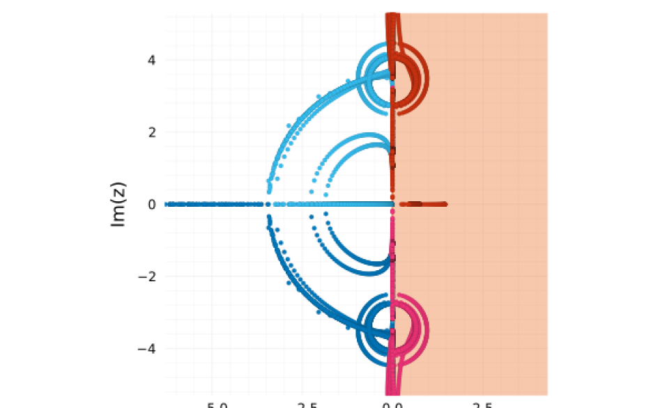
Figure 13. Friction instability. Eigenvalues of $\partial\boldsymbol{\mathrm{F}}/\partial\boldsymbol{\mathrm{u}}$ are plotted on the complex plane against the stability region of BE with $h=$ 4e-5 s. Each frame of the simulation corresponds to 4 eigenvalues, plotted here in 4 different colors, although some eigenvalues lie well outside the plotted region. Here $k=10$ N/m, $m=1$ kg, $\mu=1.2$, $\kappa=100$ N/m, $\delta=0.4$ m and $\epsilon=0.01$ m/s so that the free end of the rod repeatedly goes in and out of contact. This transition causes eigenvalues to fall into the unstable region, however it does not destabilize the overall simulation.

Increasing the time step, will reduce the number of eigenvalues in the unstable region for BE as errors are damped and the stability region expands, however, for non-L-stable integrators like TR, the errors are not damped with time step increase and so more eigenvalues remain in the unstable region throughout the simulation.

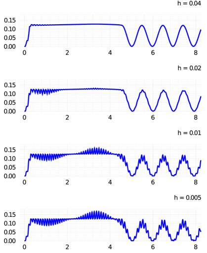
Time (s) A smooth energy plot at the top is shown h = 0.04 seconds, followed by 3 plots for h = 0.02, 0.01, and 0.005 seconds, which show more vertical zig-zags in the plot.

Figure 14. Kinetic energy of the 2D rod example is plotted for different time steps. High frequency oscillations emerge as time step $h$ is decreased. We used TR-BDF2 here, although other converging integrators exhibit similar behavior. TR will exhibit the high frequency oscillations even for $h=0.04$ s, while BE requires time steps as low as $h=$ 1e-4 s before these artifacts become visible.

In the next instance we disable damping and set $v_{s}=-0.5$ m/s, $k=15$ N/m, $m=1$ kg, $\mu=0.2$, $\kappa=10^{3}$ N/m, $\delta=0.01$ m, and $\epsilon=0.01$ m/s to demonstrate how the 2D elastic rod behaves when subject to smooth frictional contacts. In Figure 14 we plot the kinetic energy of the system as $h$ is decreased to reveal the high frequency oscillations that characterize smooth frictional contact. Consider the latter part of the animation in Figure 14, when the rod is dragged. As the conveyor belt pulls on the rod, the elastic force pulls the mass up, thus decreasing the normal force experienced. As a result, the friction force is decreased and eventually the rod accelerates in the positive direction. This causes the “large” oscillations in Figure 14. Now because our contact is enabled by a smooth but steep potential, the rod is effectively bouncing up and down at a very high frequency, which causes high frequency changes to the friction force. This causes the “small” oscillations.

Appendix B Volume change penalty formulas

In this section we briefly describe how to derive the volume penalties for ideal gas and nearly incompressible fluid given in Eqs. (18) and (19) respectively.

Assuming hydrostatic equilibrium, the mechanical potential of a fluid body can be expressed as the work done on the system when being compressed or expanded from $V$ to $V+dV$.

$$dW=-PdV,$$

where $P$ is the pressure of the fluid. Since we simulate objects in an atmosphere, the work done on a system is offset by the atmospheric pressure acting on the system. At the scale of our simulations, the atmospheric pressure is approximately constant, so the work that can affect the rest of the simulation is given by

(33) $$dW=-P+P_{0}\,dV,$$

where $P_{0}=$ 1 atm is the atmospheric pressure.

B.1. Ideal gas

For an ideal gas, Boyle’s law dictates that $PV$ is constant, which implies that it can be computed from atmospheric pressure and rest volume $PV=P_{0}V_{0}$. Thus, from Eq. (33), the energy of the system undergoing a change of volume from $V_{0}$ to $V_{1}$ can be written as

$$W(V_{1}) =\int_{V_{0}}^{V_{1}}\!-P(V)+P_{0}\,dV=P_{0}\int_{V_{0}}^{V_{1}}\!1-\frac{V_{0}}{V}\,dV$$

$$=P_{0}\left(V_{1}-V_{0}\left(1+\ln\frac{V_{1}}{V_{0}}\right)\right).$$

B.2. Nearly incompressible fluid

Recall the compressibility coefficient $\kappa_{v}$ defined by Eq. (17) for nearly incompressible fluids. The pressure change of a bounded fluid caused by volume change from $V_{0}$ to $V_{1}$ can be expressed in terms of $\kappa_{v}$ as

$$P(V_{1})-P(V_{0})=\int_{V_{0}}^{V_{1}}\!\frac{\partial P}{\partial V}dV=-\int_{V_{0}}^{V_{1}}\!\frac{dV}{\kappa_{v}V}=-\frac{1}{\kappa_{v}}\ln\frac{V_{1}}{V_{0}}.$$

With $P_{0}=P(V_{0})$, we can then derive the expression for energy directly as follows

$$W(V_{1}) =\int_{V_{0}}^{V_{1}}\!-P(V)+P_{0}\,dV=\int_{V_{0}}^{V_{1}}\frac{1}{\kappa_{v}}\ln\frac{V}{V_{0}}\,dV$$

$$=\frac{1}{\kappa_{v}}\left(\int_{V_{0}}^{V_{1}}\!\ln V\,dV-(V_{1}-V_{0})\ln V_{0}\right)$$

$$=\frac{1}{\kappa_{v}}\left(V_{0}-V_{1}\left(1-\ln\frac{V_{1}}{V_{0}}\right)\right).$$

References

- (1)
- Anderson (2018) Matt Anderson. 2018. Tennis ball hitting the wall at 100 mph. https://www.youtube.com/watch?v=FC8Tpi3U0H0
- Ascher et al. (2022) Uri M. Ascher, Egor Larionov, Seung Heon Sheen, and Dinesh K. Pai. 2022. Simulating deformable objects for computer animation: A numerical perspective. Journal of Computational Dynamics 9, 2 (2022), 47–68.
- Ascher and Petzold (1998) Uri M Ascher and Linda R Petzold. 1998. Computer methods for ordinary differential equations and differential-algebraic equations. Vol. 61. Siam.
- Awrejcewicz et al. (2008) J Awrejcewicz, D Grzelczyk, and Yu Pyryev. 2008. 404. A novel dry friction modeling and its impact on differential equations computation and Lyapunov exponents estimation. Journal of Vibroengineering 10, 4 (2008).
- Baraff and Witkin (1998) David Baraff and Andrew Witkin. 1998. Large steps in cloth simulation. In Proceedings of the 25th annual conference on Computer graphics and interactive techniques. ACM, 43–54.
- Bender et al. (2017) Jan Bender, Matthias Müller, and Miles Macklin. 2017. A Survey on Position Based Dynamics, 2017. In EUROGRAPHICS 2017 Tutorials. Eurographics Association.
- Bertails-Descoubes et al. (2011) Florence Bertails-Descoubes, Florent Cadoux, Gilles Daviet, and Vincent Acary. 2011. A nonsmooth Newton solver for capturing exact Coulomb friction in fiber assemblies. ACM Transactions on Graphics (TOG) 30, 1 (2011), 6.
- Bezanson et al. (2012) Jeff Bezanson, Stefan Karpinski, Viral B Shah, and Alan Edelman. 2012. Julia: A fast dynamic language for technical computing. arXiv preprint arXiv:1209.5145 (2012).
- Bouaziz et al. (2014) Sofien Bouaziz, Sebastian Martin, Tiantian Liu, Ladislav Kavan, and Mark Pauly. 2014. Projective Dynamics: Fusing Constraint Projections for Fast Simulation. ACM Trans. Graph. 33, 4, Article 154 (July 2014), 11 pages. https://doi.org/10.1145/2601097.2601116
- Brown et al. (2018) George E. Brown, Matthew Overby, Zahra Forootaninia, and Rahul Narain. 2018. Accurate Dissipative Forces in Optimization Integrators. ACM Trans. Graph. 37, 6, Article 282 (dec 2018), 14 pages. https://doi.org/10.1145/3272127.3275011
- Ciarlet (1983) Philippe G. Ciarlet. 1983. Lectures on three-dimensional elasticity. Vol. 71.;71;. published for the Tata Institute of Fundamental Research [by] Springer, Berlin.
- Daviet et al. (2011) Gilles Daviet, Florence Bertails-Descoubes, and Laurence Boissieux. 2011. A hybrid iterative solver for robustly capturing coulomb friction in hair dynamics. ACM Transactions on Graphics (TOG) 30, 6, 139.
- De Saxcé and Feng (1998) G. De Saxcé and Z. Q. Feng. 1998. The bipotential method: A constructive approach to design the complete contact law with friction and improved numerical algorithms. Mathematical and Computer Modelling 28, 4 (Aug. 1998), 225–245. https://doi.org/10.1016/S0895-7177(98)00119-8
- Eisenstat and Walker (1996) Stanley C. Eisenstat and Homer F. Walker. 1996. Choosing the Forcing Terms in an Inexact Newton Method. SIAM Journal on Scientific Computing 17, 1 (1996), 16–32. https://doi.org/10.1137/0917003 arXiv:https://doi.org/10.1137/0917003
- Erleben (2017) Kenny Erleben. 2017. Rigid Body Contact Problems Using Proximal Operators. In Proceedings of the ACM SIGGRAPH / Eurographics Symposium on Computer Animation (Los Angeles, California) (SCA ’17). ACM, New York, NY, USA, Article 13, 12 pages. https://doi.org/10.1145/3099564.3099575
- Geilinger et al. (2020) Moritz Geilinger, David Hahn, Jonas Zehnder, Moritz Bächer, Bernhard Thomaszewski, and Stelian Coros. 2020. ADD: analytically differentiable dynamics for multi-body systems with frictional contact. ACM Transactions on Graphics 39, 6 (Nov. 2020), 1–15. https://doi.org/10.1145/3414685.3417766
- Géradin et al. (1993) Michel Géradin, Daniel Rixen, M Géradin, and D Rixen. 1993. Théorie des vibrations: application à la dynamique des structures. Vol. 2. Masson Paris.
- Goodyear (2020) Goodyear. 2020. NHRA Drag Race Tire Wrinkle in Slow Motion — Top Fuel and Funny Car. https://www.youtube.com/watch?v=gXp2QgY1OB8
- Hughes and Knovel (2000) Thomas J. R. Hughes and General Engineering & Project Administration Knovel, Academic. 2000. The finite element method: linear static and dynamic finite element analysis. Dover Publications, Mineola, NY.
- Kane et al. (2000) C. Kane, J. E. Marsden, M. Ortiz, and M. West. 2000. Variational integrators and the Newmark algorithm for conservative and dissipative mechanical systems. Internat. J. Numer. Methods Engrg. 49, 10 (2000), 1295–1325. https://doi.org/10.1002/1097-0207(20001210)49:10<1295::AID-NME993>3.0.CO;2-W
- Kaufman et al. (2008) Danny M. Kaufman, Shinjiro Sueda, Doug L. James, and Dinesh K. Pai. 2008. Staggered Projections for Frictional Contact in Multibody Systems. ACM Transactions on Graphics (SIGGRAPH Asia 2008) 27, 5 (2008), 164:1–164:11.
- Kaufman et al. (2014) Danny M. Kaufman, Rasmus Tamstorf, Breannan Smith, Jean-Marie Aubry, and Eitan Grinspun. 2014. Adaptive nonlinearity for collisions in complex rod assemblies. ACM Transactions on Graphics (TOG) 33, 4 (2014), 123.
- Kikuuwe et al. (2005) R. Kikuuwe, N. Takesue, A. Sano, H. Mochiyama, and H. Fujimoto. 2005. Fixed-step friction simulation: from classical Coulomb model to modern continuous models. In 2005 IEEE/RSJ International Conference on Intelligent Robots and Systems. IEEE, Edmonton, Alta., Canada, 1009–1016. https://doi.org/10.1109/IROS.2005.1545579
- Larionov (2022) Egor Larionov. 2022. autodiff. https://github.com/elrnv/autodiff
- Larionov et al. (2021) Egor Larionov, Ye Fan, and Dinesh K. Pai. 2021. Frictional Contact on Smooth Elastic Solids. ACM Trans. Graph. 40, 2, Article 15 (April 2021), 17 pages. https://doi.org/10.1145/3446663
- Li et al. (2018) Jie Li, Gilles Daviet, Rahul Narain, Florence Bertails-Descoubes, Matthew Overby, George E Brown, and Laurence Boissieux. 2018. An implicit frictional contact solver for adaptive cloth simulation. ACM Transactions on Graphics (TOG) 37, 4 (2018), 52.
- Li et al. (2020) Minchen Li, Zachary Ferguson, Teseo Schneider, Timothy Langlois, Denis Zorin, Daniele Panozzo, Chenfanfu Jiang, and Danny M. Kaufman. 2020. Incremental Potential Contact: Intersection- and Inversion-free Large Deformation Dynamics. ACM Transactions on Graphics 39, 4 (2020).
- Löschner et al. (2020) Fabian Löschner, Andreas Longva, Stefan Jeske, Tassilo Kugelstadt, and Jan Bender. 2020. Higher‐Order Time Integration for Deformable Solids. Computer Graphics Forum 39, 8 (Dec. 2020), 157–169. https://doi.org/10.1111/cgf.14110
- Macklin et al. (2019) Miles Macklin, Kenny Erleben, Matthias Müller, Nuttapong Chentanez, Stefan Jeschke, and Viktor Makoviychuk. 2019. Non-smooth Newton Methods for Deformable Multi-body Dynamics. ACM Transactions on Graphics 38, 5 (Oct 2019), 1–20. https://doi.org/10.1145/3338695
- Macklin et al. (2016) Miles Macklin, Matthias Müller, and Nuttapong Chentanez. 2016. XPBD: Position-Based Simulation of Compliant Constrained Dynamics. In Proceedings of the 9th International Conference on Motion in Games (Burlingame, California) (MIG ’16). Association for Computing Machinery, New York, NY, USA, 49–54. https://doi.org/10.1145/2994258.2994272
- Mandl (1971) F. Mandl. 1971. Statistical physics. Wiley, London;New York;.
- Müller et al. (2007) Matthias Müller, Bruno Heidelberger, Marcus Hennix, and John Ratcliff. 2007. Position based dynamics. Journal of Visual Communication and Image Representation 18, 2 (2007), 109–118.
- Newmark (1959) Nathan M. Newmark. 1959. A Method of Computation for Structural Dynamics. Journal of the Engineering Mechanics Division 85, 3 (1959), 67–94. https://doi.org/10.1061/JMCEA3.0000098 arXiv:https://ascelibrary.org/doi/pdf/10.1061/JMCEA3.0000098
- Nocedal and Wright (2006) Jorge Nocedal and Stephen J. Wright. 2006. Numerical Optimization (second ed.). Springer New York, New York, NY.
- Online Community (2021) Blender Online Community. 2021. Blender - a 3D modelling and rendering package. Blender Foundation, Stichting Blender Foundation, Amsterdam. http://www.blender.org
- Sheen et al. (2021) Seung H. Sheen, Egor Larionov, and Dinesh K. Pai. 2021. Volume Preserving Simulation of Soft Tissue with Skin. Proceedings of the ACM on computer graphics and interactive techniques 4, 3 (2021), 1–23.
- Sifakis and Barbic (2012) Eftychios Sifakis and Jernej Barbic. 2012. FEM Simulation of 3D Deformable Solids: A Practitioner’s Guide to Theory, Discretization and Model Reduction. In ACM SIGGRAPH 2012 Courses (Los Angeles, California) (SIGGRAPH ’12). ACM, New York, NY, USA, Article 20, 50 pages. https://doi.org/10.1145/2343483.2343501
- Smith et al. (2018) Breannan Smith, Fernando De Goes, and Theodore Kim. 2018. Stable Neo-Hookean Flesh Simulation. ACM Trans. Graph. 37, 2, Article 12 (mar 2018), 15 pages. https://doi.org/10.1145/3180491
- Terzopoulos et al. (1987) Demetri Terzopoulos, John Platt, Alan Barr, and Kurt Fleischer. 1987. Elastically Deformable Models. SIGGRAPH Comput. Graph. 21, 4 (aug 1987), 205–214. https://doi.org/10.1145/37402.37427
- van der Vorst (1992) H. A. van der Vorst. 1992. Bi-CGSTAB: A Fast and Smoothly Converging Variant of Bi-CG for the Solution of Nonsymmetric Linear Systems. SIAM J. Sci. Stat. Comput. 13, 2 (March 1992), 631–644. https://doi.org/10.1137/0913035
- Wang et al. (2011) Huamin Wang, James F. O’Brien, and Ravi Ramamoorthi. 2011. Data-driven elastic models for cloth: modeling and measurement. In ACM SIGGRAPH 2011 papers on - SIGGRAPH ’11. ACM Press, Vancouver, British Columbia, Canada, 1. https://doi.org/10.1145/1964921.1964966
- Wojewoda et al. (2008) Jerzy Wojewoda, Andrzej Stefański, Marian Wiercigroch, and Tomasz Kapitaniak. 2008. Hysteretic effects of dry friction: modelling and experimental studies. Philosophical Transactions of the Royal Society A: Mathematical, Physical and Engineering Sciences 366, 1866 (March 2008), 747–765. https://doi.org/10.1098/rsta.2007.2125