Class-Specific Attention (CSA) for Time-Series Classification

Abstract

Most neural network-based classifiers extract features using several hidden layers and make predictions at the output layer by utilizing these extracted features. We observe that not all features are equally pronounced in all classes; we call such features class-specific features. Existing models do not fully utilize the class-specific differences in features as they feed all extracted features from the hidden layers equally to the output layers. Recent attention mechanisms allow giving different emphasis (or attention) to different features, but these attention models are themselves class-agnostic. In this paper, we propose a novel class-specific attention (CSA) module to capture significant class-specific features and improve the overall classification performance of time series. The CSA module is designed in a way such that it can be adopted in existing neural network (NN) based models to conduct time series classification. In the experiments, this module is plugged into five start-of-the-art neural network models for time series classification to test its effectiveness by using 40 different real datasets. Extensive experiments show that an NN model embedded with the CSA module can improve the base model in most cases and the accuracy improvement can be up to 42%. Our statistical analysis show that the performance of an NN model embedding the CSA module is better than the base NN model on 67% of MTS and 80% of UTS test cases and is significantly better on 11% of MTS and 13% of UTS test cases.

I Introduction

Time series analysis (e.g., classification, anomaly detection) is becoming more critical in applications that collect increasing amount of time series data. Different neural network (NN)-based approaches, such as Long Short-Term Memory (LSTM) model [1], Convolutional Neural Networks (CNNs) [2], have been introduced for time series analysis. Fully-Convolutional Networks (FCN) are considered as a strong baseline in time series classification [3]. Most neural network models, either CNN or LSTM based, have several hidden layers (e.g., convolutional layers or LSTM layers) to generate temporal features – only the last several layers (e.g., global pooling layers or fully-connected layers) are used as output layers to make predictions [4, 5, 6, 2, 7].

Naturally, each extracted feature may not equally contribute to the time series classification of instances to different classes [8]: some features may be more effective for one class while other features may be more pronounced in instances of another class. If one feature mostly comes from instances in one specific class, in this paper, we refer to such feature as a class-specific feature.

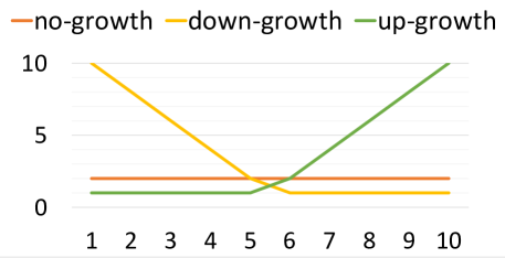
Figure 1: Toy time-series examples from different classes

Example I.1 (Class-specific features).

Fig. 1 shows the stock prices of three companies. The red curve shows the stock prices from a stable performing but no-growth company, without any price changes. The green curve shows the prices from an up-growth company and the yellow curve shows the prices of a down-growth company. It is easy to see that, in this example, the sub-sequences from time step 1 to 5 can easily separate the down-growth company from the other two; sub-sequences from 6 to 10 would be more helpful to differentiate the up-growth company from the other two companies; and the whole time range from 1 to 10 may be needed to differentiate the no-growth company from the down-growth and up-growth companies.

While the existence of class-specific features have been acknowledged and leveraged in the context of improving model explainability [8], unfortunately they are not well-utilized for the primary classification tasks by the neural networks models, which generally feed all the features generated by the hidden layers to the output layers [5, 6, 3]. TapNet [9] is the most recent model that utilizes class-label information to classify time series.

In recent years, attention mechanisms [10, 4, 11] have been introduced and widely leveraged to allow providing different levels of emphasis (or attention) to different features. Extensive research has shown that such attention mechanisms can improve the performance of neural network models in different applications. However, these attention mechanisms themselves tend to be class-agnostic and, to the best of our knowledge, for a general time-series classification task, no existing attention mechanism explicitly incorporates class-specific features for generating emphasis.

To make use of the class-specific features to improve the performance of general NN models to classify time series data, this paper proposes a novel Class-Specific Attention (CSA) module that captures class-specific features to learn class-specific attention, without negatively impacting the testing phase. The CSA is designed to give emphasis (using attention) to different class-specific features and differentiates the features that are particularly important to specific classes from the features that commonly occur in instances for all the classes. The CSA module is different from existing attention designs [10, 11, 4] because CSA utilizes class labels to calculate attention.

The main contributions of this paper are:

• We propose a Class-Specific Attention (CSA) module to capture class-specific features and learn class-specific attention from (multivariate) time series data. This module is general and can be adopted in most neural network based models that are designed for time series classification (with or without attention) to improve their performance.

• We design a Class-differentiation (CD) component to better identify the specific and important features to one class. The CSA module learns class-specific features in the hidden layers during training and can be easily used in testing.

• The CSA module is applied to five state-of-the-art neural network models on 40 real datasets (28 multivariate time-series (MTS) and 12 univariate time-series (UTS)). Extensive experiments show that a model with CSA module provides better overall performance (with accuracy improvement up to $42\%$) compared to the same model without CSA. Statistical analysis shows that the CSA module improves a base model on 67% of MTS tests and 80% of the UTS tests, is significantly better than a base base on 11% of MTS and 13% of UTS tests.

The rest of this paper is organized as follows. Section II discusses the related works. Section III presents the architecture, the learning algorithm, and the utilization of the newly proposed CSA module. Section IV reports our experimental results to evaluate the performance of the CSA module. Section V concludes this work and discusses future directions.

II Related Works

Time series classification is a well-studied problem with extensive literature on the topic. Recently, deep learning models have shown great success in time series classification. Convolutional Neural Networks (CNNs) have been exploited in time series classification because shallow convolutional layers can capture short-term temporal dependencies and deep convolutional layers can encode long-term temporal dependencies. Various CNN models are designed to classify multivariate time series data [2, 7]. In [3], a Fully-Convolutional Network (FCN) is proposed. It is considered as a strong baseline for time series classification. Different from traditional CNN models, FCN contains a group of convolutional layers without any pooling operations to prevent overfitting. Features from the convolutional layers are fed into a global averaged pooling layer to make predictions.

Other than neural networks using convolutional operations, the Long Short-Term Memory (LSTM) [1, 12, 13] and Gated Recurrent Unit (GRU) [14] based models are also widely used in temporal analysis. LSTM is one specific type of Recurrent Neural Network (RNN) models and GRU is a simpler and faster version of LSTM with similar performance. Both LSTM and GRU capture temporal features and makes predictions by using gating functions in their dynamics states.

To make good use of the FCN and LSTM models, Karim et al. [5, 6] further propose two state-of-the-art models, LSTM-FCN and MLSTM-FCN, by combining both FCN and LSTM to classify uni-variate and multivariate time series.

Recently, the attention mechanism [10] has been widely deployed on neural network classifiers to solve various types of problems. The design of the attention mechanism is motivated by human visual attention. For example, when looking at an image or reading a sentence, a human can focus on some regions (with “high resolution”) in an image or some keywords in a sentence. Similarly, utilizing attention design in neural networks can help the model to focus on more important features and pay less attention to other features. Attention is first designed in image recognition domain because it is motivated by how a human pays visual attention to different regions of an image. In recent years, attention mechanisms have been applied to language translation [11], speech recognition [15], and time series analysis [4, 5, 6, 13]. In attention mechanisms, the features of input data are kept in a hidden key space and a hidden value space (e.g., key-value pairs for a database of research articles). Given a user request (e.g., target sentence in natural language translation domain) or query (e.g., user queries in retrieval systems), the request features are represented in the hidden query space. Attention values are calculated using the similarity of the key features and the query features and are applied to adjust the features in the hidden value space. Given a group of features, attention can be used to evaluate the feature importance based on different queries. Despite all the success that attention mechanisms bring, existing attention mechanisms cannot be directly applied to capture class-specific features.

Using class-label information in classification models has been explored. Some works ([8] and [16]) apply class information for well-trained models to improve either the model explainability or the classification performance. TapNet [9] uses class label information to build a prototype (a component inside their model) for each class; they average the features of the instances for the same class label and apply softmax on the different prototypes. This is different from our design of calculating attention from class-specific key and query features [10].

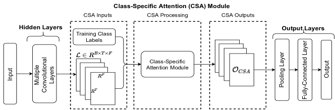
Figure 2: The overview of a FCN Model, extended with Class-Specific Attention (CSA)

III Class-Specific Attention (CSA)

It is possible that features generated from hidden layers of neural network models do not equally contribute to classifying different classes. Furthermore, features that are important to classify instances belonging to one class may not be useful in classifying instances belonging to other classes [8]. This phenomenon becomes more obvious in time-series classification when a sub-sequence of a time series, instead of the whole sequence, is more useful to classify instances from specific classes (as in Eg. I.1). In this section, we describe a Class-Specific Attention (CSA) module that builds on the above observations to identify and leverage class-specific features in time series classification.

III-A Overall Design

We explain the core idea and overall design of the CSA module using Fig. 2. The CSA module is designed in a way such that it can be adopted in existing neural network (NN) based time series classification models. Without loss of generality, we use the FCN [3] model as a representative NN model to explain the design of our newly proposed CSA module. In this figure, the CSA module is used to extend the FCN model for time series classification for illustration purposes. The CSA module is shown in the three dotted-line boxes at the center of the figure. Note that, while CSA can be placed after any hidden layer of a neural network model, in this figure (and in the experiments reported in the paper), we place it after the last hidden layer of the neural model, as later layers capture more higher-level features than the previous layers [8]. CSA takes a special form of input that leverages the class label information of training instances – such labels are generally used by existing neural network models for evaluating the loss value from the output layer, but are not explicitly utilized for learning hidden features. In contrast to the state-of-the-art, the CSA input data integrates class label information of training instances with the features learned from previous hidden layers.

CSA gives different attention (or emphasis) to features generated in the hidden layers to learn class-specific features, which are then used to evaluate the probabilities of the data instances belonging to different classes. The design of CSA adopts the basic idea of self-attention mechanism [11] where the features in the three hidden spaces (key, value, query) are learned from the same input data. On the other hand, CSA differs from self-attention mechanisms in two major aspects:

• First, CSA is designed to learn the class-specific features in the training stage and preserve these features in the hidden query space. Yet, the design of the query space, which encodes the class-specific features, can be directly utilized in the testing stage without knowing the class labels of testing instances.

• Typical attention mechanisms calculate attention values by using the similarity between the key features and the query features; however, such a calculation cannot differentiate features that commonly exist in all the instances from the class-specific features that only exist in instances of specific classes. In contrast, attention calculation in the CSA module differentiates the importance of class-specific features from other features.

Table I lists the symbols used in the method description.

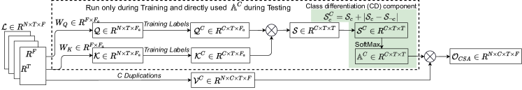
$\otimes$ denotes matrix multiplication and $\oplus$ denotes matrix addition

Figure 3: The architecture of the Class-Specific Attention (CSA) Module – notation convention: (1) A symbol using AMS blackboard bold font ($\mathbb{A}^{C}$) represents a tensor learned from training instances, and directly used for testing; (2) the other tensors are represented using math calligraphic font style (e.g., $\mathcal{L}$, $\mathcal{K}$, $\mathcal{V}$, $\mathcal{S}$); (3) class-specific tensors are denoted with a superscript $C$ (e.g., $\mathcal{Q}^{C}$, $\mathcal{K}^{C}$, $\mathcal{V}^{C}$, $\mathcal{S}^{C}$); (4) kernel weights are represented using $W$ with a subscript ($W_{Q}$, $W_{K}$); (5) dimension sizes are represented as superscript for $R$ (e.g., $R^{N\times T}$).

Symbol	Meaning
$N$	# of instances in a TS dataset
$C$	# of distinct classes in a dataset
$V$	# of variables in a TS dataset
$T$	# of time points of one time series in $X$
$\mathcal{L}$	Feature matrix from hidden layers
$F$	# of features at each time point in $X$
$F_{a}$	# of features in the hidden key and query spaces
$B$	# of instances in one batch

TABLE I: Symbols used in this paper

Algorithm 1 CSA_Calculation

Input: $\mathcal{L}\in R^{N\!\times\!T\!\times\!F}$: feature tensor from the hidden layers
Output: $\mathcal{O}_{CSA}\in R^{N\!\times\!C\!\times\!T\!\times F}$: feature tensor adjusted using class-specific attention

1:   $\mathcal{K}=\mathcal{L}\cdot W_{K}$ where $W_{K}\in R^{F\times F_{a}}$

2:   $\mathcal{Q}=\mathcal{L}\cdot W_{Q}$ where $W_{Q}\in R^{F\times F_{a}}$

3:  Initialize $\mathcal{K}^{C}\in R^{C\!\times T\!\times F},\mathcal{Q}^{C}\in R^{C\!\times T\!\times F}$

4:  for each class label $c$ do

5:     $\mathcal{L}_{c}$ = all the instances belonging to class $c$.

6:      $\mathcal{K}^{C}[c,:,:]=average(\mathcal{K}[\mathcal{L}_{c},:,:]$) on the first dimension

7:      $\mathcal{Q}^{C}[c,:,:]=average(\mathcal{Q}[\mathcal{L}_{c},:,:])$ on the first dimension

8:  end for

9:  $\mathcal{S}=\mathcal{K}^{C}\cdot(\mathcal{Q}^{C})^{T}$ where $\mathcal{S}\in R^{C\times T\times T}$

10:  Initialize $\mathcal{S}^{C}\in R^{C\!\times T\!\times T}$

11:  for each class label $c$ do

12:     $\mathcal{S}_{c}=\mathcal{S}[c,:,:]$

13:     $\mathcal{S}_{\neg c}=\frac{SUM(\mathcal{S})-\mathcal{S}_{c}}{C-1}$

14:      $\mathcal{S}^{C}[c,:,:]=\mathcal{S}_{c}+abs(\mathcal{S}_{c}-\mathcal{S}_{\neg c})$

15:  end for

16:   $\mathbb{A}^{C}=SoftMax(\mathcal{S}^{C})\in R^{C\!\times T\!\times T}$

17:   $\mathcal{V}=\mathcal{L}\cdot W_{V}$, where $W_{V}\in R^{F\times F}$

18:  $\mathcal{V}^{C}=$ shape $C$ copies of $\mathcal{V}$ to $R^{N\times C\times T\times F}$

19:  $\mathcal{L}^{C}=$ shape $C$ copies of $\mathcal{L}$ to $R^{N\times C\times T\times F}$

20:  $\mathcal{O}_{CSA}=\mathcal{L}^{C}+\sigma\times(\mathbb{A}^{C}\cdot\mathcal{V}^{C})$

21:  return $\mathcal{O}_{CSA}$

III-B Overview of the CSA Architecture

The features from the hidden layers of the FCN model are fed as input to the CSA module – in particular, we assume that features are generated by the hidden layers that are immediately before the CSA module in the architecture.

The CSA architecture outlined in Fig. 3 embodies our key design decisions:

Design Decision $\#1$. Unlike the existing self-attention mechanisms, CSA introduces the class-specific attention $\mathbb{A}^{C}$ to differentiate class-specific features from other features. In particular, after learning the features $\mathcal{Q}$ and $\mathcal{K}$ in the latent query and key spaces, CSA aggregates the instances in the same class in these two feature spaces to get two class-specific feature tensors $\mathcal{Q}^{C}$ and $\mathcal{K}^{C}$ so that they can be further utilized in calculating the class-specific attention $\mathbb{A}^{C}$ and the updated features $\mathcal{O}_{CSA}$.

Design Decision $\#2$. The class-specific attention $\mathbb{A}^{C}$ is designed to be a global tensor. It is updated during the training stage and can be directly used in testing. Consequently, the CSA design avoids the need for the testing instances to have class labels.

III-C Training Process

The ultimate goal of the CSA training is to convert regular features (denoted as $\mathcal{L}$ in Fig. 3) to class-specific features ($\mathcal{O}_{CSA}$ in Fig. 3). This conversion utilizes the class-specific attention $\mathbb{A}^{C}$.

The CSA_Calculation algorithm, shown in Algorithm 1, provides an overview of the learning process for CSA training. First, for the training instances, the features in the hidden query space ($\mathcal{Q}$) and key space ($\mathcal{K}$) are learned (Lines 1-2). Then, these two feature tensors are transformed to class-specific query features $\mathcal{Q}^{C}$ and class-specific key $\mathcal{K}^{C}$ features (Lines 4-8). Next, $\mathcal{Q}^{C}$ are combined with $\mathcal{K}^{C}$ to calculate the class-specific attention $\mathbb{A}^{C}$ (Lines 9-16). Finally, the attention $\mathbb{A}^{C}$ is applied to the value features $\mathcal{V}^{C}$ (which is reshaped from the original feature tensor $\mathcal{L}$) to get $\mathcal{O}_{CSA}$ (Line 20).

In what follows, we provide details of the learning processes for calculating the class-specific attention $\mathbb{A}^{C}$.

III-C1 Generating Class-Specific Features $\mathcal{Q}^{C}$ and $\mathcal{K}^{C}$

Using the similar mechanism to learn attention models [10, 11, 4], we learn the hidden features in query space ($\mathcal{Q}$) and key space ($\mathcal{K}$). Then, the class-specific features ($\mathcal{Q}^{C}$ and $\mathcal{K}^{C}$) are generated as follows. From $\mathcal{Q}$ (or $\mathcal{K}$), the algorithm finds instances from a specific class label $c$ and averages their features to be $\mathcal{Q}^{C}$ (or $\mathcal{K}^{C}$) (Line 6-7). The first dimension of $\mathcal{Q}^{C}$ is not the number of instances ($N$) as that in $\mathcal{Q}$. It becomes the number of classes ($C$). This process can be demonstrated using an example in Fig. 4. It explains how the features specific to class 1 and class 2 are calculated.

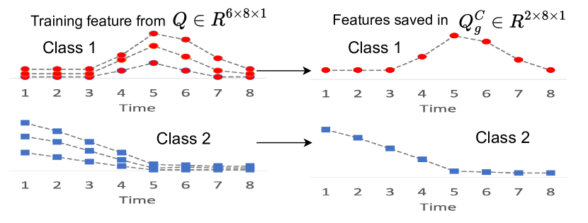
Figure 4: Example from $\mathcal{Q}$ to $\mathcal{Q}^{C}$ (The points with the same color represent the features for one specific class)

III-C2 Learning Process for $\mathbb{A}^{C}$

The calculation of the class-specific attention $\mathbb{A}^{C}$ utilizes the class-specific query features $\mathcal{Q}^{C}$ and the key features $\mathcal{K}^{C}$.

To calculate the similarity between $\mathcal{Q}^{C}$ and $\mathcal{K}^{C}$, a feature matrix is calculated as $\mathcal{S}=\mathcal{K}^{C}\cdot(\mathcal{Q}^{C})^{T}$. Different from existing attention mechanisms, we introduce a class differentiation (CD) component to post-process the feature matrix $\mathcal{S}$, as shown as the right shaded area in Fig. 3. Existing attention mechanisms calculate the attention values directly from $\mathcal{S}$. However, calculating the similarity between the key and query features is not sufficient for CSA. If a feature is learned from instances in multiple (or all) classes, finding this feature may not be very helpful when making predictions. To better separate instances from one class, CSA needs to identify specific features from instances within this class, which are not commonly found from instances belonging to other classes. By adding the absolute differences between features for class $c$ and all the other classes ($\neg c$) (Lines 11-15), we seek features that can differentiate instances from class $c$ and instances from other classes ($\neg c$) while still making use of the original features. The significant class-specific features are kept in $\mathcal{S}^{C}$. $\mathcal{S}^{C}$ is further used to calculate the class-specific attention $\mathbb{A}^{C}$ (Line 16).

III-C3 Updating of $\mathcal{L}$ to $\mathcal{O}_{CSA}$

Class-specific attention $\mathbb{A}^{C}$ is used to adjust the value features $\mathcal{V}$ from $\mathcal{L}$ to get $\mathcal{O}_{CSA}$ (Lines 17-21).

The value features $\mathcal{V}$ and the features in $\mathcal{L}$ are transformed to $\mathcal{V}^{C}$ and $\mathcal{L}^{C}$ by repeat $C$ copies. The output features in $\mathcal{O}_{CSA}$ are calculated using $\mathcal{O}_{CSA}=\mathcal{L}^{C}+\sigma\times(\mathbb{A}^{C}\cdot\mathcal{V}^{C})$ where $\sigma$ is a learnable scalar value.

III-D Utilization of CSA for the Output of NN

In the CSA-embedded FCN model (i.e., FCN model that embeds the CSA module, as shown in Figure 2), the features in $\mathcal{O}_{CSA}$ are adjusted using class-specific attention and are fed to output layers (global pooling layers and fully connected layers). More specifically, the output layers of the CSA-embedded FCN consist of one global pooling layer and one fully connected layer. The design of the global pooling layer follows the common design practice in existing models [5, 6, 3]: $\mathcal{O}_{CSA}$ ($\in R^{N\!\times\!C\!\times\!T\!\times\!F}$) is converted to a condensed feature tensor $\mathcal{G}\!\in\!R^{N\!\times\!C\!\times\!F}$ by averaging the features in the time dimension.

Dataset	$N$	$C$	$V$	T
ArtWordRec	575	25	9	144
BasicMotions	80	4	6	100
CharTraj	2858	20	3	182
Cricket	180	12	6	1197
DuckDuckGeese	100	5	270	1345
EigenWorms	259	5	6	17984
Epilepsy	275	4	3	206
EthanolConc	1751	4	3	1751
FaceDetection	9414	2	62	144
FingerMovements	416	2	28	50
HandMovement	234	4	10	400
Handwriting	1000	26	3	152
Heartbeat	409	2	61	405
InsectWingbeat	50000	10	30	200
JapaneseVowels	640	10	26	12
LSST	4925	14	6	36
Libras	360	15	2	45
MotorImagery	378	2	64	3000
NATOPS	360	6	24	51
PEMS-SF	440	7	963	144
PenDigits	10992	10	2	8
Phoneme	6668	39	11	217
RacketSports	303	4	6	30
SelfRegSCP1	561	2	6	896
SelfRegSCP2	380	2	7	1152
SpokenArab	8798	10	13	93
StandWalkJump	27	3	4	2500
UWaveGesture	440	8	3	315
MedicalImages	1141	10	1	99
MelPedestrian	3633	10	1	24
MidPhalanxoutGrp	554	3	1	80
MidPhalanxoutCor	891	2	1	80
MidPhalanxtw	553	6	1	80
OsuLeaf	442	6	1	427
PhalangesCor	2658	2	1	80
Powercons	360	2	1	144
ProximalPhaGrp	605	3	1	80
ProximalPhaCor	891	2	1	80
ProximalPhaTw	605	6	1	80
RefrigerationDev	750	3	1	720

TABLE II: Statistics of 28 MTS and 12 UTS Datasets

Where CSA differs from the conventional design is in the fully connected layer: the features in $\mathcal{G}$, if directly fed to a traditional fully connected layer, cannot make good use of the features from specific classes because fully-connected layers directly combine all features without considering their differences. Instead, we design a layer by introducing class-specific weights and biases to better utilize class-specific features. In particular, for each class $c$, a weight matrix $\Omega\in R^{F\!\times\!1}$ and a bias $\beta$ are used to calculate a value for this class ($val=\mathcal{G}\cdot\Omega\!+\!\beta$). This value is used to get the probability of an instance belonging to class $c$. Compared with the traditional fully-connected layer, this design can make better use of the class-specific features from $\mathcal{O}_{CSA}$ because features from different classes are not combined. Instead, the probability of an instance belonging to one class is calculated only using features specific to this class for most cases. Meanwhile, the weight parameters (in $\Omega$ and $\beta$) are not more than those in a traditional fully-connected layer – therefore, the training time for this fully-connected layer does not increase.

Prediction for a testing instance. The class-specific features $\mathcal{O}_{CSA}$ for a testing instance are calculated by directly utilizing the global class-specific attention $\mathbb{A}^{C}$ and the value features of this instance. Note that the testing instance does not need any class label to leverage class-specific attention. Next, these class-specific features $\mathcal{O}_{CSA}$ are passed to the specially designed fully connected layer described above to make class predictions.

IV Experiments

In this section, we evaluate the effectiveness of the proposed CSA module. In particular, we aim to answer the following questions:
(Q1) Does the CSA module improve the performance of a baseline neural network model (which may or may not implement a general attention mechanism) to classify time series data?
(Q2) Does the CD component contribute to improving the performance of the CSA module? and
(Q3) Will the CSA module introduce dramatic overheads (regarding training time) in the model learning process?

All methods are implemented using $Python~{}3.7$ and tested on a server with Intel Xeon Gold 5218 2.3G CPUs, 192GB RAM, and one Nvidia Tesla V100 GPU with 32GB memory. PyTorch 1.10 is used to build all the models. To acquire stable results, every number (accuracy or running time) we report is an average of five runs.

IV-A Experimental Settings

Datasets. We report results on 40 datasets, where 28 MTS datasets are from the UEA repository [17] and 12 UTS datasets are from the UCR repository [18]. Two datasets from the UEA are not utilized because they have too few instances and the UTS datasets are randomly chosen.

Methods for Comparison. The CSA module is designed to be compatible with, and improve the time series classification performance of, existing neural network (NN) models. Many neural network models exist to classify time series, it is not realistic to embed CSA to all of them for testing. In our experiments, we embed the CSA module in five representative state-of-the-art models, namely (1) Fully Convolutional Networks (FCN) [3], (2) Multivariate Long Short-Term Memory (MLSTM) [1], (3) MLSTM-FCN [6], (4) CNN with attention (CNN-ATN) [4], and (5) TapNet [9]. The first three models are widely used NN models without attention mechanism, while CNN-ATN leverages attention in MTS classification, TapNet incorporates both attention and class label information in training. For these five models, we get their implementation from the published source code. If the code version is not comparable, we convert the code to PyTorch. Recall that the CSA module implements a CD component. To evaluate the effectiveness of the CD component of the CSA module, we implement a CSA module without the CD component for testing.

Hyper-Parameter Setting. We use the hyper-parameter settings reported in [6], and [4]: the convolutional layers of the FCN model contain three 1D kernels with sizes 8, 5, 3 – the corresponding numbers of kernels are 128, 256, and 128. The pooling filter in the global pooling layer has the same as the length as the time series output from the previous layer. The 2D kernels in the CNN-ATN model have sizes ($8\times 1$), ($5\times 1$), and ($3\times 1$). The number of the hidden states of MLSTM model is 128. The $F$ parameter for $\mathcal{L}$ (Fig. 3) for all the models is set to 128. For TapNet, the number of variable subsets is set to 3. We do not test the effect of these hyper-parameters because they are intrinsic in the base models, but not the CSA module. Tuning the parameters to get good performance is not the focus of this paper. We use settings that are the same or similar to their original papers.

Evaluation Measure. We report a commonly used classification performance measure, accuracy ($Acc\in[0,1]$), because most datasets are balanced. We also compute and report the accuracy improvement, $AI$, to compare two models, $A$ and $B$, with accuracy values $Acc_{A}$ and $Acc_{B}$:

$$AI(A,B)=\frac{Acc_{A}-Acc_{B}}{Acc_{B}}$$ (1)

Since we are generally interested in measuring the improvement provided by the CSA module over the conventional baselines, we use $AI_{\text{\em Model}}$ to denote $AI(\text{{\em Model-CSA}},\text{{\em Model}})$. Each experiment were run five times on each dataset and the average accuracy and improvements for each dataset are reported.

We also conduct statistical analysis, the null hypothesis testing [19], to gain a more in-depth understanding of the effectiveness of the CSA module. Given one dataset, the null hypothesis is that the Model-CSA performs similarly with (not significantly better than) the base Model. The $p$-value is calculated using the Chi-Square Test [20]. If $p$-value is bigger than a threshold (a commonly used threshold is 0.05), the null hypothesis is rejected and we consider the model with higher accuracy is significantly better than the other model.

IV-B Effectiveness Analysis

This section presents the effectiveness of the CSA module.

IV-B1 MTS datasets

We first study the effectiveness of plugging CSA to a neural network model on classifying MTS datasets. We report the detailed accuracy/AI values in Table III. For each model, the first two columns (‘w/o CSA’ and ‘w CSA’ show the accuracy of the models and the third column (‘AI’) shows the accuracy improvement of Model-CSA over the base Model. Table V also uses this convention.

In this table, the results on several datasets for TapNet and CNN-ATN model are missing (denoted with ’-’) because these models cannot finish utilizing the GPU memory. CNN-ATN uses 2D convolutional operations, as well as attentions over variable and temporal dimensions, which requires a large memory space. TapNet generates an $\mathcal{L}$ tensor from three subsets of the input MTS data, thus utilizes much more space.

	FCN			MLSTM			MLSTM-FCN
Datasets	w/o CSA	w CSA	AI	w/o CSA	w CSA	AI	w/o CSA	w CSA	AI
ArtWordRec	0.980	0.982	0.204	0.816	0.856	4.902	0.972	0.982	1.029
BasicMotions	0.968	0.966	-0.207	0.844	0.852	0.948	0.966	0.968	0.207
CharTraj	0.990	0.990	0.000	0.974	0.980	0.616	0.992	0.996	0.403
Cricket	0.910	0.910	0.000	0.704	0.708	0.568	0.878	0.896	2.050
DuckDuckGeese	0.740	0.766	3.514	0.672	0.694	3.274	0.722	0.734	1.662
EigenWorms	0.544	0.552	1.471	0.464	0.464	0.000	0.526	0.574	9.125
Epilepsy	0.794	0.842	6.045	0.666	0.686	3.003	0.864	0.874	1.157
EthanolConc	0.624	0.658	5.449	0.342	0.346	1.170	0.622	0.654	5.145
FaceDetection	0.562	0.562	0.000	0.578	0.582	0.692	0.556	0.562	1.079
FingerMovements	0.648	0.656	1.235	0.614	0.614	0.000	0.642	0.642	0.000
HandMovement	0.468	0.488	4.274	0.370	0.414	11.892	0.466	0.492	5.579
Handwriting	0.284	0.288	1.408	0.208	0.224	7.692	0.282	0.296	4.965
Heartbeat	0.812	0.818	0.739	0.818	0.820	0.244	0.810	0.816	0.741
InsectWingbeat	0.108	0.138	27.778	0.124	0.124	0.000	0.116	0.136	17.241
JapaneseVowels	0.882	0.890	0.907	0.938	0.952	1.493	0.932	0.934	0.215
LSST	0.444	0.456	2.703	0.528	0.530	0.379	0.530	0.558	5.283
Libras	0.902	0.906	0.443	0.552	0.708	28.261	0.906	0.902	-0.442
MotorImagery	0.640	0.648	1.250	0.608	0.624	2.632	0.638	0.638	0.000
NATOPS	0.886	0.898	1.354	0.792	0.820	3.535	0.882	0.898	1.814
PEMS-SF	0.930	0.946	1.720	0.576	0.704	22.222	0.928	0.944	1.724
PenDigits	0.984	0.982	-0.203	0.976	0.976	0.000	0.980	0.980	0.000
Phoneme	0.088	0.092	4.545	0.100	0.106	6.000	0.096	0.114	18.750
RacketSports	0.748	0.774	3.476	0.778	0.790	1.542	0.770	0.804	4.416
SelfRegSCP1	0.872	0.874	0.229	0.898	0.904	0.668	0.884	0.888	0.452
SelfRegSCP2	0.568	0.586	3.169	0.572	0.596	4.196	0.592	0.592	0.000
SpokenArab	0.974	0.982	0.821	0.960	0.960	0.000	0.982	0.986	0.407
StandWalkJump	0.400	0.400	0.000	0.692	0.652	-5.780	0.428	0.414	-3.271
UWaveGesture	0.624	0.618	-0.962	0.814	0.820	0.737	0.768	0.766	-0.260
Averaged			2.549			3.603			2.838

	TapNet			CNN-ATN
Datasets	w/o CSA	w CSA	AI	w/o CSA	w CSA	AI
ArtWordRec	0.980	0.988	0.816	0.984	0.988	0.407
BasicMotions	1.000	0.994	-0.600	0.982	1.000	1.833
CharTraj	0.990	0.990	0.000	0.990	0.990	0.000
Cricket	0.950	0.932	-1.895	0.808	0.826	2.228
DuckDuckGeese	0.724	0.676	-6.630	-	-	-
EigenWorms	0.600	0.580	-3.333	-	-	-
Epilepsy	0.870	0.822	-5.517	0.950	0.954	0.421
EthanolConc	0.322	0.364	13.043	0.520	0.510	-1.923
FaceDetection	0.562	0.570	1.423	-	-	-
FingerMovements	0.614	0.636	3.583	0.602	0.620	2.990
HandMovement	0.464	0.520	12.069	0.422	0.442	4.739
Handwriting	0.198	0.278	40.404	0.296	0.298	0.676
Heartbeat	0.748	0.732	-2.139	0.820	0.820	0.000
InsectWingbeat	-	-	-	-	-	-
JapaneseVowels	0.988	0.992	0.405	0.990	0.990	0.000
LSST	0.450	0.642	42.667	0.664	0.674	1.506
Libras	0.790	0.820	3.797	0.790	0.790	0.000
MotorImagery	0.636	0.614	-3.459	-	-	-
NATOPS	0.890	0.890	0.000	0.946	0.950	0.423
PEMS-SF	0.912	0.912	0.000	-	-	-
PenDigits	0.940	0.940	0.000	0.970	0.970	0.000
Phoneme	0.164	0.216	31.707	-	-	-
RacketSports	0.704	0.816	15.909	0.888	0.888	0.000
SelfRegSCP1	0.736	0.636	-13.587	0.830	0.878	5.783
SelfRegSCP2	0.578	0.590	2.076	0.546	0.558	2.198
SpokenArab	0.982	0.982	0.000	0.990	0.990	0.000
StandWalkJump	0.508	0.588	15.748	-	-	-
UWaveGesture	0.882	0.874	-0.907	0.838	0.834	-0.477
Averaged			5.392			1.040

TABLE III: Comparison of models with and w/o CSA on MTS

	Model-CSA is Better
Base Model	Significantly	Not Significantly	Total
FCN	3/28	18/28	21/28
MLSTM	2/28	20/28	22/28
MLSTM-FCN	4/28	17/28	21/28
TapNet	5/27	8/27	13/27
CNN-ATN	1/20	10/20	11/20
Percentages	15/131	73/131	88/131
of test cases	=11.45%	=55.73%	=67.18%

TABLE IV: Statistical significance analysis for all the models on MTS datasets ($p$-value threshold: 0.05; Each test case is for one dataset being applied with a base model and its CSA counterpart.

	FCN			LSTM			LSTM-FCN
Datasets	w/o CSA	w CSA	AI	w/o CSA	w CSA	AI	w/o CSA	w CSA	AI
MedicalImages	0.792	0.794	0.253	0.522	0.580	11.111	0.786	0.790	0.509
MelPedestrian	0.660	0.666	0.909	0.830	0.900	8.434	0.796	0.798	0.251
MidPhalanxoutGrp	0.604	0.636	5.298	0.428	0.580	35.514	0.618	0.616	-0.323
MidPhalanxoutCor	0.814	0.816	0.246	0.570	0.570	0.000	0.810	0.812	0.247
MidPhalanxtw	0.516	0.516	0.000	0.458	0.554	20.961	0.500	0.516	3.200
OsuLeaf	0.966	0.974	0.828	0.210	0.210	0.000	0.964	0.976	1.245
PhalangesCor	0.804	0.806	0.249	0.600	0.600	0.000	0.798	0.806	1.003
Powercons	0.926	0.930	0.432	0.940	0.952	1.277	0.926	0.932	0.648
ProximalPhaGrp	0.838	0.846	0.955	0.590	0.738	25.085	0.840	0.842	0.238
ProximalPhaCor	0.846	0.864	2.128	0.690	0.720	4.348	0.834	0.860	3.118
ProximalPhaTw	0.744	0.728	-2.151	0.734	0.824	12.262	0.718	0.744	3.261
RefrigerationDev	0.520	0.516	-0.769	0.408	0.464	13.725	0.528	0.536	1.515
Averaged			0.644			11.251			1.175

	TapNet			CNN-ATN
Datasets	w/o CSA	w CSA	AI	w/o CSA	w CSA	AI
MedicalImages	0.750	0.752	0.267	0.766	0.774	1.044
MelPedestrian	0.792	0.822	3.788	0.850	0.862	1.412
MidPhalanxoutGrp	0.658	0.662	0.608	0.668	0.682	2.096
MidPhalanxoutCor	0.844	0.848	0.474	0.826	0.828	0.242
MidPhalanxtw	0.618	0.610	-1.294	0.540	0.542	0.370
OsuLeaf	0.972	0.982	1.029	0.898	0.916	2.004
PhalangesCor	0.772	0.790	2.332	0.806	0.822	1.985
Powercons	0.944	0.960	1.695	0.918	0.928	1.089
ProximalPhaGrp	0.856	0.854	-0.234	0.850	0.852	0.235
ProximalPhaCor	0.894	0.900	0.671	0.918	0.908	-1.089
ProximalPhaTw	0.794	0.800	0.756	0.818	0.828	1.222
RefrigerationDev	0.584	0.584	0.000	0.582	0.568	-2.405
Averaged			0.776			0.631

TABLE V: Comparison of models with and w/o CSA on UTS

The table clearly show that the AI values is bigger than zero for most datasets for each base model. This means that the CSA module helps improve all these different base models. The average AI for the different models ranges from 1.04% to 5.39%. There are a few cases where the base models show slightly better performance than their corresponding CSA model; we conjecture that this is due to the increase in the number of model parameters when using the CSA extension.

The accuracy improvement over the TapNet method is the highest. This is because TapNet generates the $\mathcal{L}$ tensor from three subsets of the input MTS data, which is three times larger than the $\mathcal{L}\in R^{N\times T\times F}$ from other models. The large $\mathcal{L}$ provides more information for our CSA module to utilize.

The statistical analysis is conducted on all 28 MTS datasets. Table IV presents the results. The first five rows present the percentage of datasets and the last row shows the percentage of all test cases, where each test case is for one dataset being applied with a base model and its CSA counterpart. There are $28$ MTS datasets with 5 different base NN models. Ideally, the total number of test cases is $28\times 5=140$. However, TapNet can only finish 27 datasets and CNN-ATN can only finish 20 datasets. The total number of available test cases is 131 ($28+28+28+27+20$). Among all the 131 cases, in $11.45\%$ (15/131) cases, the Model-CSA significantly outperform the base Model. The Model-CSA is better but not statistically significant better than the Model in $55.73\%$ cases. Overall, Model-CSA is better than Model in $67.18\%$ cases.

IV-B2 UTS datasets

Table V presents the accuracy/AI values on UTS for all the models. The results show that the proposed CSA module can also improve the classification performance of all the base models on UTS datasets. The average AI for the different models ranges from 0.6% to 11% Compared with the results on the MTS datasets, the AI results are slightly smaller on UTS datasets. This is because MTS datasets normally have more features than the UTS datasets.

	Model-CSA is Better
Base Model	Significantly	Not Significantly	Total
FCN	0/12	9/12	9/12
LSTM	7/12	2/12	9/12
LSTM-FCN	0/12	11/12	11/12
TapNet	1/12	8/12	9/12
CNN-ATN	0/12	10/12	10/12
Percentages	8/60	40/60	48/60
of test cases	=13.33%	=66.67%	=80.00%

TABLE VI: Statistical significance analysis for all the models on UTS datasets ($p$-value threshold: 0.05; Each test case is for one dataset being applied with a base model and its CSA counterpart)

We want to particular mention that the improvement on the TapNet model is low on UTS. The reason is that there is only one variable in a UTS. Thus, we cannot create multiple variable subsets to generate $\mathcal{L}$. The best improvement is observed on the LSTM model (which corresponds to the MLSTM model for MTS). This is because LSTM is the worst performing base model on UTS, which can be observed from the accuracy values in the ‘LSTM w/o CSA’ column .

We also conduct the null hypothesis test on the UTS datasets. We run the tests on all the 12 UTS datasets and present the results in Table VI. Again, since we test on five models, there are 60 test cases ($5\times 12$). In about $13.33\%$ cases, a model with CSA significantly outperforms the base model and, in $66.67\%$ cases, there is improvement (although not statistically significant). The total percentage of benefited cases from the CSA module is $80\%$. On UTS datasets, the majority improvements are from the LSTM model, it might be because that the LSTM model has relatively lower performance on the 12 UTS datasets.

Similar with the conclusion on MTS datasets, Model-CSA reports better performance than the base Model on UTS datasets. In the rest of the experimental sections, we present the results from tests on the MTS datasets to avoid redundant contents.

IV-C Ablation Study

	FCN-CSA
Datasets	w/o CD	w CD	AI
ArtWordRec	0.980	0.982	0.204
BasicMotions	0.962	0.966	0.416
CharTraj	0.990	0.990	0.000
Cricket	0.914	0.910	-0.438
DuckDuckGeese	0.742	0.766	3.235
EigenWorms	0.562	0.552	-1.780
Epilepsy	0.818	0.842	2.997
EthanolConc	0.658	0.658	0.000
FaceDetection	0.560	0.562	0.357
FingerMovements	0.653	0.656	0.536
HandMovement	0.475	0.488	2.737
Handwriting	0.280	0.288	2.857
Heartbeat	0.813	0.818	0.677
InsectWingbeat	0.134	0.138	2.985
JapaneseVowels	0.890	0.890	0.000
LSST	0.478	0.456	-4.50
Libras	0.896	0.906	1.116
MotorImagery	0.642	0.648	0.935
NATOPS	0.898	0.898	0.000
PEMS-SF	0.943	0.946	0.371
PenDigits	0.980	0.982	0.204
Phoneme	0.086	0.092	6.977
RacketSports	0.764	0.774	1.309
SelfRegSCP1	0.886	0.874	-1.354
SelfRegSCP2	0.573	0.586	2.358
SpokenArab	0.972	0.982	1.029
StandWalkJump	0.418	0.400	-4.192
UWaveGesture	0.612	0.618	0.980
Averaged			0.715
Wins			19/28

TABLE VII: Comparison for FCN-CSA models with and w/o CD component on MTS datasets

CSA relies on a class-differentiation (CD) component to detect the features that can differentiate a class $c$ and the remaining ones $\neg c$. In order to assess the impact of the CD component, we implement a version of CSA without CD, Model-CSA-NoCD as follows. We calculate the CSA outputs by applying the SoftMax function directly on $\mathcal{S}$ to calculate $\mathcal{A}^{C}$, without calculating the feature differences between class $c$ and classes $\neg c$ (i.e., without computing $\mathcal{S}^{C}_{c}$ and $\mathcal{S}^{C}$ in Fig. 3). Without loss of generality, we choose one base model (FCN model) and run FCN-CSA and FCN-CSA-NoCD over all the MTS datasets. As we expect, for most data sets, the CD component helps improve the performance. As shown in Table VII, on average, FCN-CSA increase the accuracy of FCN-CSA-NoCD with 0.72%. Despite that this number is not big, we note that among all the MTS datasets, FCN-CSA outperforms FCN-CSA-NoCD on 19 datasets and they have same performance on 4 datasets. These results show that the CD component helps improve the time series classification performance in general.

	K Nearest Neighbor
Dataset	classifier with DTWd	MLSTM-FCN-CSA
ArtWordRec	0.987	0.982
BasicMotions	0.975	0.968
CharTraj	0.99	0.996
Cricket	1	0.896
DuckDuckGeese	0.6	0.734
EigenWorms	0.618	0.574
Epilepsy	0.964	0.874
EthanolConc	0.323	0.654
FaceDetection	0.529	0.562
FingerMovements	0.53	0.642
HandMovement	0.231	0.492
Handwriting	0.607	0.296
Heartbeat	0.717	0.816
InsectWingbeat	0.12	0.136
JapaneseVowels	0.949	0.934
LSST	0.872	0.558
Libras	0.551	0.902
MotorImagery	0.5	0.638
NATOPS	0.883	0.898
PEMS-SF	0.711	0.944
PenDigits	0.977	0.98
Phoneme	0.151	0.114
RacketSports	0.803	0.804
SelfRegSCP1	0.775	0.888
SelfRegSCP2	0.539	0.592
SpokenArab	0.963	0.986
StandWalkJump	0.2	0.414
UWaveGesture	0.903	0.766
Averaged	0.677	0.715
Wins		18/28

TABLE VIII: Accuracy comparison between K nearest neighbor classifier (with DTW_d for distance calculation) and MLTSM-FCN-CSA on MTS datasets

IV-D Case Study: Comparison with non-NN methods

The propose CSA module can help improve the performance of neural network-based models, but cannot be leveraged in the traditional time-series classification methods, such as the K-Nearest-Neighbor classifier [21], Dynamic Time Warping (DTW) [22]. The K-Nearest-Neighbor approach has shown excellent performance in classifying time series [23, 17]. In particular, 1-Nearest-Neighbor classifier with dimension-dependent DTW (DTW_d) [17] is considered as a strong baseline for the non-NN based method to classify MTS datasets. In this section, we compare the performance of one neural network model which embeds the CSA module and the 1-Nearest-Neighbor classifier (with DTW_d) to show that the neural network based models with CSA generally outperform the Nearest-Neighbor approaches. Without loss of generality and to save space, we use MLSTM-FCN-CSA as a representative for the neural network models with the CSA module. Note that the performance of the other NN-CSA models can be obtained from Table III.

Table VIII shows the classification accuracy values of the two models. As shown in the table, the MLSTM-FCN-CSA performs better than the Nearest-Neighbor method (DTW_d) on most datasets (18/28) and has better averaged accuracy. Please be aware that optimizing the training of an NN-based model is not the focus of this paper. The results in this section are from a relatively small number of training epochs (400). The effect of the training epochs is analyzed in Section IV-F.

IV-E Case Study: Visual Examples of Class-Specific Features

We conduct a case study to present the class-specific features using an example. It is challenging to generate user friendly feature examples from deep learning models. Please note that optimally visualizing deep learning features is not the focus of this work.

We present two feature matrices ($P^{L}$ and $P^{O}$), before and after the CSA module, to show how the CSA module changes the regular features to class-specific features in one training batch (with batch size $B$). $P^{L}$ and $P^{O}$ are post-processed from $\mathcal{L}$ and $\mathcal{O}^{CSA}$ in Fig. 3. $P^{L}$ is obtained by conducting an average pooling over the $T$ dimension of $\mathcal{L}\in R^{B\times T\times F}$. Thus, its size is $B\times F$. Similarly, $P^{O}$ is generated from the average pooling over the $T$ dimension on $\mathcal{Q_{CSA}}$, and has size $B\times C\times F$. For each training instance, $P^{O}$ has $C$ feature sequences whose length is $F$, while $P^{L}$ has only one feature sequence with length $F$.

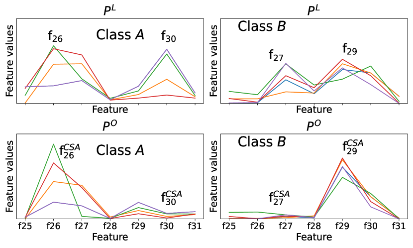
(a) Feature comparisons for class A and B

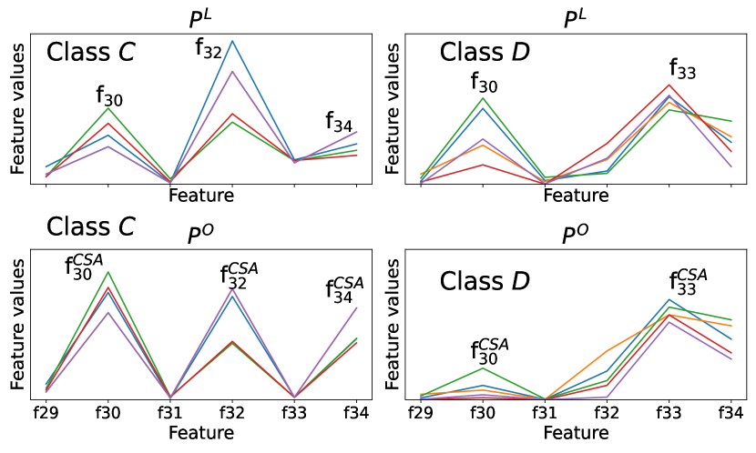
(b) Feature comparisons for class C and D

Figure 5: Feature comparisons (5 random instances are drawn in different colors; first row plots regular features, second row plots class-specific features.)

For a specific class $c$, we compare the differences between the $c$th feature sequences (for $B$ instances) in $P^{O}$ with the feature sequences (for the same $B$ instances) in $P^{L}$. Fig. 5 presents the comparison between two pairs of example classes. To improve the readability, we randomly pick 5 instances (in one batch) from classes $A$ and $B$, and only show a subset of features ($f_{25}$ to $f_{31}$).

We can see from the plotted features that the CSA module can emphasize some features (with higher values) and weaken other features (with lower values). E.g., In Fig. 5(a), feature $f_{30}$ is weakened (lower values) by the CSA module for class A and feature $f_{29}$ is emphasized by the CSA module for class B. The CSA module may change the importance of features. For example, in Fig. 5(b), $f_{30}$ was less important (smaller) than $f_{32}$ in the original feature space. However, the CSA module makes the $f_{30}^{CSA}$ more important (with higher value) than $f_{32}^{CSA}$.

	FCN trained with 400 epochs			FCN trained with 800 epochs			FCN trained with 1200 epochs
Datasets	w/o CSA	w CSA	AI	w/o CSA	w CSA	AI	w/o CSA	w CSA	AI
ArtWordRec	0.980	0.982	0.204	0.980	0.986	0.612	0.980	0.986	0.612
BasicMotions	0.968	0.966	-0.207	0.956	0.974	1.883	0.968	0.980	1.240
CharTraj	0.990	0.990	0.000	0.990	0.990	0.000	0.990	0.990	0.000
Cricket	0.910	0.910	0.000	0.900	0.928	3.111	0.912	0.928	1.754
DuckDuckGeese	0.740	0.766	3.514	0.750	0.746	-0.533	0.750	0.750	0.000
EigenWorms	0.544	0.552	1.471	0.566	0.586	3.534	0.580	0.590	1.724
Epilepsy	0.794	0.842	6.045	0.828	0.832	0.483	0.844	0.856	1.422
EthanolConc	0.624	0.658	5.449	0.646	0.674	4.334	0.660	0.686	3.939
FaceDetection	0.562	0.562	0.000	0.562	0.564	0.356	0.566	0.568	0.353
FingerMovements	0.648	0.656	1.235	0.640	0.646	0.938	0.642	0.650	1.246
HandMovement	0.468	0.488	4.274	0.472	0.474	0.424	0.456	0.484	6.140
Handwriting	0.284	0.288	1.408	0.290	0.302	4.138	0.290	0.298	2.759
Heartbeat	0.812	0.818	0.739	0.812	0.820	0.985	0.814	0.818	0.491
InsectWingbeat	0.108	0.138	27.778	0.104	0.130	25.000	0.100	0.142	42.000
JapaneseVowels	0.882	0.890	0.907	0.880	0.891	1.250	0.886	0.894	0.903
LSST	0.444	0.456	2.703	0.462	0.472	2.165	0.476	0.488	2.521
Libras	0.902	0.906	0.443	0.908	0.908	0.000	0.896	0.908	1.339
MotorImagery	0.640	0.648	1.250	0.642	0.646	0.623	0.658	0.680	3.343
NATOPS	0.886	0.898	1.354	0.898	0.900	0.223	0.900	0.904	0.444
PEMS-SF	0.930	0.946	1.720	0.942	0.948	0.637	0.946	0.950	0.423
PenDigits	0.984	0.982	-0.203	0.984	0.982	-0.203	0.982	0.980	-0.204
Phoneme	0.088	0.092	4.545	0.094	0.098	4.255	0.100	0.092	-8.000
RacketSports	0.748	0.774	3.476	0.776	0.788	1.546	0.770	0.788	2.338
SelfRegSCP1	0.872	0.874	0.229	0.886	0.866	-2.257	0.870	0.874	0.460
SelfRegSCP2	0.568	0.586	3.169	0.572	0.586	2.448	0.574	0.582	1.394
SpokenArab	0.974	0.982	0.821	0.976	0.984	0.820	0.976	0.980	0.410
StandWalkJump	0.400	0.400	0.000	0.414	0.480	15.942	0.440	0.522	18.636
UWaveGesture	0.624	0.618	-0.962	0.612	0.614	0.327	0.622	0.612	-1.608
Averaged			2.549			2.609			3.074

TABLE IX: Comparison of FCN and FCN-CSA with different number of epochs

IV-F Study of the Effect of Parameters

In this section, we study the effectiveness of the proposed CSA with different training epochs. There are many other neural network parameters, such as the number of layers, and the number of neurons, which are used to define the model architecture. We do not study the architecture parameters since optimizing the network structure is an open question and is not the focus of this paper. With the same model architecture (Model and Model-CSA), we would like to examine whether the AI improves with the increase of the number of epochs. We use FCN in this section as a representative neural network model.

In addition to the initial number of epochs (400) used in the training (to report all the previous results), we increase the epoch number to 800 and 1200. Table IX presents the accuracy and AI results from FCN and FCN-CSA models. The results show that the performance improvements from the CSA module are consistent with all 3 epoch numbers. It means that the CSA module indeed learns novel and helpful features, which cannot be well learned by the base FCN model even with more training epochs.

For a given individual dataset, it is not guaranteed that the model has better performance with higher epoch numbers. The CSA improvements (accuracy and AI) are not monotonically increasing with the increase of epoch numbers. This is caused by the slight instability of deep-learning models after the model converges. However, the overall (averaged) results over all MTS datasets (last row in Table IX) with higher epoch number get better than the results with lower epoch.

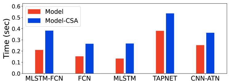
(a) Training time per iteration
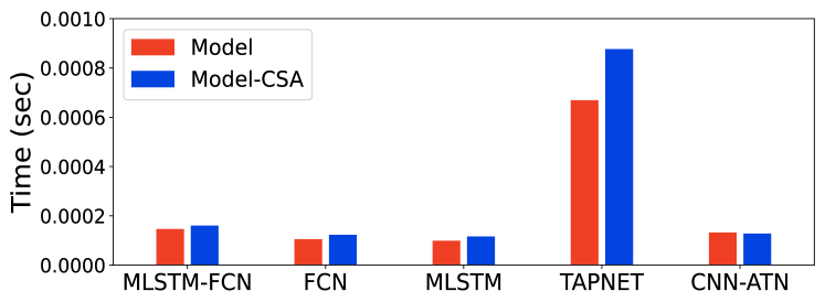
(b) Testing time per instance

Figure 6: Running time (averaged on all the datasets)

IV-G Efficiency Analysis

The above results show that class-specific attention generally has positive impact on classification accuracy. In this section, we examine the efficiency of the proposed CSA module.

Fig. 6 (a) reports the training time for the baseline models (i.e., Model) and Model-CSA per iteration. As we would expect, CSA requires additional time to calculate the tensors and learning parameters in the CSA architecture. Model-CSA uses up to 0.2 seconds more than Model to train the models in one iteration. While class-specific attention has an impact on training times, there are no significant differences between the testing times of baseline models with models extended with CSA. Fig. 6 (b) shows Model-CSA uses almost the same time as Model to make predictions for one instance for all models except TapNet. TapNet has a bigger difference because it has more features (three times) than other models to learn in the CSA module. This confirms that class-specific attention can be used effectively in practice for accurate time series classification.

V Conclusions and Future Works

This paper presents a class-specific attention (CSA) module to improve the performance of neural network models for time series classification. The proposed module can be embedded to neural network models for time series classification (including those that leverage other forms of attention) to automatically capture significant features to differentiate instances of one class from the instances of the other classes. CSA identifies class-specific features leveraging training labels, while avoiding the need to access label information during testing phase. To the best of our knowledge, this is the first attention design that leverages the class label information in the hidden layers to generate class-specific features. Experiments on 40 real datasets have shown that CSA generally boosts accuracy – in the experiments, we have seen performance improvements up to 42%. Statistical analysis shows that the CSA module improves a base neural network model on 67% of MTS tests and 80% of the UTS tests, is significantly better than a base base on 11% of MTS and 13% of UTS tests.

To make the tests more extensive, we can apply the models on more time series datasets (e.g., all the UTS datasets in the UCR repository). As a further step, the same design principle of CSA module can be utilized to improve the classification performance of other types of data such as images.

References

- [1] S. Hochreiter and J. Schmidhuber, “Long short-term memory,” Neural Computation, vol. 9, no. 8, pp. 1735–1780, 1997. [Online]. Available: https://doi.org/10.1162/neco.1997.9.8.1735
- [2] J. Yang, M. N. Nguyen, P. P. San, X. Li, and S. Krishnaswamy, “Deep convolutional neural networks on multichannel time series for human activity recognition,” in IJCAI, 2015, pp. 3995–4001. [Online]. Available: http://ijcai.org/Abstract/15/561
- [3] Z. Wang, W. Yan, and T. Oates, “Time series classification from scratch with deep neural networks: A strong baseline,” in International Joint Conference on Neural Networks (IJCNN), 2017, pp. 1578–1585. [Online]. Available: https://doi.org/10.1109/IJCNN.2017.7966039
- [4] Y. Hao and H. Cao, “A new attention mechanism to classify multivariate time series,” in IJCAI, 2020, pp. 1999–2005. [Online]. Available: https://doi.org/10.24963/ijcai.2020/277
- [5] F. Karim, S. Majumdar, H. Darabi, and S. Chen, “LSTM fully convolutional networks for time series classification,” IEEE Access, vol. 6, pp. 1662–1669, 2018. [Online]. Available: https://doi.org/10.1109/ACCESS.2017.2779939
- [6] F. Karim, S. Majumdar, H. Darabi, and S. Harford, “Multivariate lstm-fcns for time series classification,” Neural Networks, vol. 116, pp. 237–245, 2019. [Online]. Available: https://doi.org/10.1016/j.neunet.2019.04.014
- [7] Y. Zheng, Q. Liu, E. Chen, Y. Ge, and J. L. Zhao, “Exploiting multi-channels deep convolutional neural networks for multivariate time series classification,” Frontiers Comput. Sci., vol. 10, no. 1, pp. 96–112, 2016. [Online]. Available: https://doi.org/10.1007/s11704-015-4478-2
- [8] Y. Hao, H. Cao, A. Mueen, and S. Brahma, “Identify significant phenomenon-specific variables for multivariate time series,” IEEE Trans. Knowl. Data Eng., vol. 31, pp. 1–13, 2019.
- [9] X. Zhang, Y. Gao, J. Lin, and C. Lu, “Tapnet: Multivariate time series classification with attentional prototypical network,” in The Thirty-Fourth Conference on Artificial Intelligence, AAAI 2020, February 7-12, 2020, 2020, pp. 6845–6852. [Online]. Available: https://aaai.org/ojs/index.php/AAAI/article/view/6165
- [10] D. Bahdanau, K. Cho, and Y. Bengio, “Neural machine translation by jointly learning to align and translate,” in ICLR, 2015. [Online]. Available: http://arxiv.org/abs/1409.0473
- [11] A. Vaswani, N. Shazeer, N. Parmar, J. Uszkoreit, L. Jones, A. N. Gomez, L. Kaiser, and I. Polosukhin, “Attention is all you need,” in Annual Conference on Neural Information Processing Systems 2017, 2017, pp. 5998–6008. [Online]. Available: http://papers.nips.cc/paper/7181-attention-is-all-you-need
- [12] R. Pascanu, Ç. Gülçehre, K. Cho, and Y. Bengio, “How to construct deep recurrent neural networks,” in 2nd International Conference on Learning Representations (ICLR), 2014. [Online]. Available: http://arxiv.org/abs/1312.6026
- [13] Y. Qin, D. Song, H. Chen, W. Cheng, G. Jiang, and G. W. Cottrell, “A dual-stage attention-based recurrent neural network for time series prediction,” in IJCAI, 2017, pp. 2627–2633. [Online]. Available: https://doi.org/10.24963/ijcai.2017/366
- [14] K. Cho, B. van Merrienboer, D. Bahdanau, and Y. Bengio, “On the properties of neural machine translation: Encoder-decoder approaches,” CoRR, vol. abs/1409.1259, 2014. [Online]. Available: http://arxiv.org/abs/1409.1259
- [15] C. Shan, J. Zhang, Y. Wang, and L. Xie, “Attention-based end-to-end speech recognition in mandarin,” CoRR, vol. abs/1707.07167, 2017. [Online]. Available: http://arxiv.org/abs/1707.07167
- [16] Y. Hao, H. Cao, and E. Draayer, “Cnn approaches to classify multivariate time series using class-specific features,” in 2020 IEEE International Conference on Smart Data Services (SMDS), 2020, pp. 1–8.
- [17] A. Bagnall, H. A. Dau, J. Lines, M. Flynn, J. Large, A. Bostrom, P. Southam, and E. Keogh, “The UEA multivariate time series classification archive, 2018,” 2018.
- [18] Y. Chen, E. Keogh, B. Hu, N. Begum, A. Bagnall, A. Mueen, and G. Batista, “The ucr time series classification archive,” July 2015, www.cs.ucr.edu/~eamonn/time_series_data/.
- [19] C. Pernet, “Null hypothesis significance testing: a short tutorial,” F1000Research, vol. 4, 08 2015.
- [20] K. Pearson, “X. on the criterion that a given system of deviations from the probable in the case of a correlated system of variables is such that it can be reasonably supposed to have arisen from random sampling,” The London, Edinburgh, and Dublin Philosophical Magazine and Journal of Science, vol. 50, no. 302, pp. 157–175, Jul. 1900. [Online]. Available: https://doi.org/10.1080/14786440009463897
- [21] A. Mucherino, P. J. Papajorgji, and P. M. Pardalos, k-Nearest Neighbor Classification. New York, NY: Springer New York, 2009, pp. 83–106. [Online]. Available: https://doi.org/10.1007/978-0-387-88615-2_4
- [22] T. Giorgino, “Computing and visualizing dynamic time warping alignments in R: The dtw package,” Journal of Statistical Software, vol. 31, no. 7, pp. 1–24, 2009.
- [23] H. Ding, G. Trajcevski, P. Scheuermann, X. Wang, and E. J. Keogh, “Querying and mining of time series data: experimental comparison of representations and distance measures,” Proc. VLDB Endow., vol. 1, no. 2, pp. 1542–1552, 2008. [Online]. Available: http://www.vldb.org/pvldb/vol1/1454226.pdf