Eigenvalue Analysis and Applications of the Legendre Dual-Petrov-Galerkin Methods for Initial Value Problems

Abstract.

In this paper, we show that the eigenvalues and eigenvectors of the spectral discretisation matrices resulted from the Legendre dual-Petrov-Galerkin (LDPG) method for the $m$th-order initial value problem (IVP): $u^{(m)}(t)=\sigma u(t),\,t\in(-1,1)$ with constant $\sigma\not=0$ and usual initial conditions at $t=-1,$ are associated with the generalised Bessel polynomials (GBPs). The essential idea of the analysis is to properly construct the basis functions for the solution and its dual spaces so that the matrix of the $m$th derivative is an identity matrix, and the mass matrix is then identical or approximately equals to the Jacobi matrix of the three-term recurrence of GBPs with specific integer parameters. This allows us to characterise the eigenvalue distributions and identify the eigenvectors. As a by-product, we are able to answer some open questions related to the very limited known results on the collocation method at Legendre points (studied in 1980s) for the first-order IVP, by reformulating it into a Petrov-Galerkin formulation. Moreover, we present two stable algorithms for computing zeros of the GBPs, and develop a general space-time spectral method for evolutionary PDEs using either the matrix diagonalisation, which is restricted to a small number of unknowns in time due to the ill-conditioning but is fully parallel, or the QZ decomposition which is numerically stable for a large number of unknowns in time but involves sequential computations. We provide ample numerical results to demonstrate the high accuracy and robustness of the space-time spectral methods for some interesting examples of linear and nonlinear wave problems.

1. Introduction

Spectral methods are a class of numerical methods which use global orthogonal polynomials/functions as basis functions, and have gained much popularity due to its high accuracy for problems with solutions that are smooth in suitable functional spaces [2, 3, 20]. However, spectral methods are mostly used in spatial discretisations, while time discretisations are usually done with traditional approaches such as implicit-explicit schemes or explicit Runge-Kutta methods which are of fixed-order convergence rates, thus creating a mismatch between spectral accuracy in space and usually lower-order accuracy in time. In practice, space-time spectral methods are attractive for problems with dynamics that require high resolution in both space and time, e.g., oscillatory wave propagations.

Several attempts have been made in developing spectral methods in time. Tal-Ezer [23, 24] first studied Chebyshev spectral methods in time for linear hyperbolic and parabolic problems. Tang and Ma [25] presented a Legendre-tau spectral method in time for parabolic PDEs with periodic boundary conditions in space; and later in [26] for hyperbolic problems in a similar setting. Shen and Wang [10] proposed a Fourierization space-time Legendre spectral method for parabolic equations. Recently, Lui [13] investigated a space-time Legendre spectral collocation method for the heat equation. Shen and Sheng [19] developed a space-time dual-Petrov-Galerkin method for fractional (in time) subdiffusion equations and adopted a QZ decomposition technique to overcome the extreme ill-conditioning when the eigen-decomposition is used. However, a theoretical foundation for such methods is still lacking. It is known that the eigenvalue distribution of the spectral differentiation matrices plays a central role in the stability and round-off error of the underlying spectral method. While the eigenvalue distribution of spectral approximation to second-order BVPs were well established [7, 30, 1, 31], very little is known about the eigenvalue distribution of spectral approximation to IVPs; particularly no results appear available for higher-order IVPs.

Unlike the second-order operators for BVPs, spectral approximations to the derivative operators of IVPs can be problematic. In particular, the derivative matrices are usually non-normal, which typically require more stringent conditions for the stability. We refer to Gottlieb and Orszag [8] for insightful stability analysis of spectral approximations to first-order hyperbolic problems, and briefly review the existing findings (mostly on asymptotic eigenvalue analysis of first-order spectral discretisation matrices in 1980s). Dubiner [6] conducted an asymptotic analysis of the spectral-tau method for a prototype problem: find $\lambda\in{\mathbb{C}}$ and $u_{N}\in{\mathbb{P}}_{N}={\rm span}\{x^{k}:0\leq k\leq N\}$ such that

$$u_{N}^{\prime}(x)-\lambda u_{N}(x)=p_{N}(x),\;\;\;x\in(-1,1);\quad u_{N}(1)=0,$$ (1.1)

where $p_{N}(x)$ is a polynomial of degree $N.$ In particular, for the Jacobi-tau approximation:

$$\int_{-1}^{1}\big{(}u_{N}^{\prime}-\lambda u_{N}\big{)}(x)v(x)(1-x)^{\alpha}(1+x)^{\beta}{\rm d}x=0,\quad\forall\,v\in{\mathbb{P}}_{N-1},$$

we have $p_{N}(x)=\tau P_{N}^{(\alpha,\beta)}(x)$ (with any constant $\tau\not=0$), in view of the orthogonality of Jacobi polynomials and $u_{N}^{\prime}-\lambda u_{N}\in{\mathbb{P}}_{N}.$ Dubiner [6] showed that for $\beta>-1,$

$$\lambda_{i}^{N}=O(N^{2}),\;\;{\rm if}\;\;\alpha\in(-1,1];\quad\lambda_{i}^{N}=O(N),\;\;{\rm if}\;\;\alpha=0.$$

According to [4], all eigenvalues lie in the left half-plane. Following [6], Wang and Waleffe [28] further proved the existence of unstable eigenvalues for $\alpha>1$ and the eigenvalues of the Legendre case are zeros of the modified Bessel function $k_{N}(z)$, drawn from the property $k_{N}(z)=z^{-1}{{\rm e}^{-z}}\sum_{k=0}^{N}{P_{N}^{(k)}(1)}{z^{-k}}$ and its relation with the characteristic polynomial of (1.1).

Tal-Ezer [22], and Trefethen and Trummer [27] discovered that eigenvalues of the spectral differentiation matrix of the collocation methods for the first-order IVP at the Legendre points (see (3.11)) behave like $\lambda_{i}^{N}=O(N),$ but $\lambda_{i}^{N}=O(N^{2})$ at Chebyshev and other Jacobi points. Accordingly, the allowable time-step size in the explicit time discretisation of the hyperbolic problem is $O(N^{-1}),$ rather than $O(N^{-2})$ for the Chebyshev and other Jacobi collocation methods. However, numerical evidences in [27] indicated that the Legendre collocation approximation with $O(N^{-1})$ time-step constraint appeared only in theory, but subject to an $O(N^{-2})$ restriction in practice. Moreover, the computation of the eigenvalues is precision-dependent, and is extremely sensitive to perturbations/round-off errors, e.g., the use of EISPACK could produce reliable eigenvalues for $N\leq 28$ with double-precision calculations [27]. Here, we demonstrate in Figure 1.1 the eigenvalues computed by eig($\boldsymbol{D}$) in Matlab, where the reference eigenvalues are computed by the algorithm in Pasquini [16] for computing the zeros of the GBP (see Theorem 3.2 and Section 6). The numerical study in [27] gave rise to open questions, e.g., on the identifications of eigenvalues and eigenvectors, and rigorous proof of the exponential growth of the condition number of the eigenvector matrix.

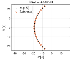
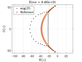
Figure 1.1. Eigenvalue distributions of the first-order differentiation matrix on Legendre points with $N=28$ (left) and $N=56$ (right). The red circles denote the reference values, and the black dots denote the eigenvalues computed in double precision.

The objective of this paper is to conduct rigorous eigenvalue analysis of the spectral matrices resulted from LDPG spectral methods for the first-order and general $m$th order IVPs. The argument of the analysis and main findings are summarized as follows.

• We properly construct the basis polynomials for the solution and dual approximation spaces so that the matrix of the highest derivative term is an identity matrix, but the mass matrix is a non-normal sparse matrix. This enables us to associate the mass matrix with the Jacobi matrix corresponding to the three-term recurrence relation of the Bessel or generalised Bessel polynomials, and then identify the eigenvalues and eigenvectors.

• We reformulate the collocation method on Legendre points (cf.​​ [22, 27]) as a Petrov-Galerkin formulation that allows us to identify eigen-pairs of the spectral differentiation matrix via the usual Bessel polynomials (BPs). Then we can answer some open questions in [27] and locate the eigenvalues from an approach different from [28].

• We introduce two techniques to effectively deal with the (fully implicit) time-discretisation by the LDPG spectral method, which include (i) diagonalisation technique; and (ii) QZ decomposition. Due to the severe ill-conditioning of the eigenvector matrix, the diagonalisation technique, which involves the inverse of the eigenvector matrix, is only numerically stable for small $N,$ so combine it with a multi-domain spectral method to march in time sequentially. On the other hand, the QZ decomposition for such non-normal matrices is numerically stable for large $N,$ and we can solve the resulted linear systems simply by backward substitutions.

Finally, we remark that there has been a continuing interest in solving evolutionary equations in a parallel-in-time (PinT) manner based on the diagonalisation technique initiated by Maday and Rønquist [14], see, for instance, a recent work [12] on a well-conditioned parallel-in-time algorithm involving the diagonalisation of a nearly skew-symmetric matrix resulted with a modified time-difference scheme. Our LDPG method with diagonalisation can be directly applied in a parallel-in-time manner, although in practice we also need to combine it with a multi-time-domain approach, since we can only deal with a relatively short time interval in parallel due to the ill-conditioning limitation mentioned above.

The rest of this paper is organised as follows. In Section 2, we collect some related properties of the GBPs and Legendre polynomials. In Section 3, we conduct eigenvalue analysis for the LDPG spectral method for the first-order IVP, and reformulate the collocation method on Legendre points [22, 27] as a Petrov-Galerkin formulation to precisely characterise the eigenvalue distributions and the associated eigenvectors. We extend the analysis to the second-order IVPs in Section 4, and higher-order IVPs in Section 5. We present two stable algorithms for computing zeros of the GBPs in Section 6. In Section 7, we develop a general framework for space-time spectral methods, and apply it to solve linear and nonlinear wave problems. We conclude the paper with some final remarks in Section 8.

2. Properties of GBPs and Legendre polynomials

The forthcoming eigenvalue analysis relies much on the GBPs, so we collect below some relevant properties, which can be found in [11, 9, 16]. We also review some properties of Legendre polynomials to be used later on. Throughout this paper, let $\mathbb{C}$ (resp. $\mathbb{R}$) be the set all complex (resp. real) numbers, and further let $\mathbb{N}=\{1,2,\cdots\}$ and $\mathbb{N}_{0}=\{0,1,2,\cdots\}.$

2.1. Generalised Bessel polynomials

For $\alpha,\beta\in{\mathbb{C}},-\alpha\not\in{\mathbb{N}}_{0}$ and $\beta\not=0,$ the GBP, denoted by $B_{n}^{(\alpha,\beta)}(z),z\in{\mathbb{C}}$, is a polynomial of degree $n$ that satisfies the second-order differential equation

$$z^{2}y^{\prime\prime}(z)+(\alpha z+\beta)y^{\prime}(z)=n(n+\alpha-1)y(z),\quad n\in{\mathbb{N}}_{0},$$ (2.1)

which has the explicit representation

$$B_{n}^{(\alpha,\beta)}(z)=\sum_{k=0}^{n}\binom{n}{k}\frac{\Gamma(n+k+\alpha-1)}{\Gamma(n+\alpha-1)}\Big{(}\frac{z}{\beta}\Big{)}^{k}.$$ (2.2)

The GBPs can be generated by the three-term recurrence relation

$$\begin{dcases}B_{n+1}^{(\alpha,\beta)}(z)=\Big{(}a_{n}^{(\alpha)}\frac{z}{\beta}+b_{n}^{(\alpha)}\Big{)}B_{n}^{(\alpha,\beta)}(z)+c_{n}^{(\alpha)}B_{n-1}^{(\alpha,\beta)}(z),\quad n\geq 1,\\ B_{0}^{(\alpha,\beta)}(z)=1,\quad B_{1}^{(\alpha,\beta)}(z)=1+\alpha\frac{z}{\beta},\end{dcases}$$ (2.3)

where

$$\begin{split}&a_{n}^{(\alpha)}=\frac{(2n+\alpha)(2n+\alpha-1)}{n+\alpha-1},\quad b_{n}^{(\alpha)}=\frac{(\alpha-2)(2n+\alpha-1)}{(n+\alpha-1)(2n+\alpha-2)},\quad\\ &c_{n}^{(\alpha)}=\frac{n(2n+\alpha)}{(n+\alpha-1)(2n+\alpha-2)}.\end{split}$$ (2.4)

Here the normalization $B_{n}^{(\alpha,\beta)}(0)=1$ is adopted.

The GBPs are orthogonal on the unit circle (see [9, p. 30]):

$$\frac{1}{2\pi{\rm i}}\int_{|z|=1}B_{m}^{(\alpha,\beta)}(z)B_{n}^{(\alpha,\beta)}(z)\rho^{(\alpha,\beta)}(z){\rm d}z=\gamma_{n}^{(\alpha,\beta)}\delta_{mn},$$ (2.5)

where the weight function and the normalization constant are given by

$$\begin{split}&\rho^{(\alpha,\beta)}(z):=\sum_{k=0}^{\infty}\frac{\Gamma(\alpha)}{\Gamma(k+\alpha-1)}\Big{(}\!-\frac{\beta}{z}\Big{)}^{k}={{}_{1}F_{1}}(1,\alpha-1;-\beta/z),\\ &\gamma_{n}^{(\alpha,\beta)}:=\frac{(-1)^{n+1}\beta\Gamma(\alpha)n!}{(2n+\alpha-1)\Gamma(n+\alpha-1)}.\end{split}$$ (2.6)

Here ${{}_{1}F_{1}}(\,)$ is the hypergeometric function.

Observe from (2.2)-(2.3) that the parameter $\beta$ plays a role as a scaling factor, and there holds

$$B_{n}^{(\alpha,-\beta)}(z)=B_{n}^{(\alpha,\beta)}(-z).$$

For simplicity, we denote the GBP with $\beta=2$ by $B_{n}^{(\alpha)}(z):=B_{n}^{(\alpha,2)}(z).$ When $\alpha=\beta=2$, the GBPs reduce to the classical Bessel polynomials (BPs), denoted by $B_{n}(z):=B_{n}^{(2,2)}(z).$ Accordingly, the recurrence relation (2.3)-(2.4) becomes

$$\begin{dcases}B_{n+1}(z)=(2n+1)zB_{n}(z)+B_{n-1}(z),\quad n\geq 1,\\ B_{0}(z)=1,\quad B_{1}(z)=1+z.\end{dcases}$$ (2.7)

Moreover, the orthogonality (2.5)-(2.6) simply reads

$$\frac{1}{2\pi{\rm i}}\int_{|z|=1}B_{m}(z)B_{n}(z){\rm e}^{-2/z}{\rm d}z=(-1)^{n+1}\frac{2}{2n+1}\delta_{mn}.$$

We summarize the most important properties on zero distributions of GBPs below.

Theorem 2.1.

Let $\alpha\in{\mathbb{R}}$ and $n+\alpha-1>0.$ Then we have the following properties.

• All zeros of $B_{n}^{(\alpha)}(z)$ are simple and conjugate of each other.

• For $\alpha\geq-1$ and $n\geq 2,$ all zeros of $B_{n}^{(\alpha)}(z)$ are in the open left half-plane.

• For $n\geq 2,$ all zeros are located in the crescent-shaped region

  $${\mathcal{R}}_{n,\alpha}^{-}:=\Big{\{}z=\rho{\rm e}^{{\rm i}\theta}\in\mathbb{C}:\frac{2}{2n+\alpha-\frac{2}{3}}<\rho\leq\frac{1-\cos\theta}{n+\alpha-1},\;\;\theta\in(-\pi,-\Theta_{n,\alpha})\cup(\Theta_{n,\alpha},\pi]\Big{\}},$$ (2.8)

  where the equal sign can be attained only $\theta=\pi,$ and

  $$\Theta_{n,\alpha}:=\arccos\Big{(}\frac{-\alpha}{2n+\alpha-2}\Big{)}.$$ (2.9)

Proof.

According to [9, Theorem 1^′], all zeros of $B_{n}^{(\alpha)}(z)$ are simple. As $B_{n}^{(\alpha)}(z)$ is a polynomial of real coefficients, its zeros are conjugate of each other. The second statement is presented in [5, Theorem 4.3]. In fact, this result is sharp in the sense that for $\alpha<-1$, the polynomial $B_{n}^{(\alpha)}(z)$ has at least one zero in the right half-plane. Moreover, as stated in [5, Theorem 5.1], all zeros of $B_{n}^{(\alpha)}(z)$ lie in the annulus

$$A(n,\alpha):=\Big{\{}z\in{\mathbb{C}}:\frac{2}{2n+\alpha-2/3}<|z|\leq\frac{2}{n+\alpha-1}\Big{\}}.$$

More precisely, they are in the left half-annulus in view of (ii). An improved upper enclosure is given by [5, Theorem 3.1]: all zeros of $B_{n}^{(\alpha)}(z)$ are confined in the cardioidal region

$$C(n,\alpha):=\Big{\{}z=r\mathrm{e}^{{\rm i}\theta}\in\mathbb{C}:0<r<\frac{1-\cos\theta}{n+\alpha-1}\Big{\}}\cup\Big{\{}\frac{-2}{n+\alpha-1}\Big{\}}.$$

Moreover, from [5, Theorem ​ 4.1], we have that all zeros of $B_{n}^{(\alpha)}(z)$ with $n\geq 2$ are in the sector

$$S(n,\alpha):=\Big{\{}z=\rho{\rm e}^{{\rm i}\theta}\in\mathbb{C}:|\theta|>\arccos\Big{(}\frac{-\alpha}{2n+\alpha-2}\Big{)},\;\;-\pi<\theta\leq\pi\Big{\}}.$$

Then we define

$${\mathcal{R}}_{n,\alpha}^{-}:=A(n,\alpha)\cap C(n,\alpha)\cap S(n,\alpha),$$

which leads to the statement (iii). ∎

Remark 2.1.

It is also noteworthy of the following properties.

• If $n\not=m,$ no zero of $B_{n}^{(\alpha)}(z)$ can be a zero of $B_{m}^{(\alpha)}(z)$, see [9, Theorem 1(b^′)].

• For any fixed $\alpha$ and for odd $n,$ let $Z_{n,\alpha}$ be the unique (negative) real zero of $B_{n}^{(\alpha)}(z).$ We find from [5, Theorem ​ 4.1] the asymptotic behaviour

  $$Z_{n,\alpha}\approx-\frac{2}{1.3254868n+1.00628995\alpha-1.34983648+O((2n+\alpha-2)^{-1})},\quad n\gg 1.$$ (2.10)

  In particular, for the BP $B_{n}(z),$ its unique real zero for odd $n$ behaves like $Z_{n,2}=-\nu n^{-1}+O(n^{-2})$ with $\nu\approx 1.50888\ldots.$

2.2. Legendre polynomials

The Legendre polynomials, denoted by $P_{n}(x)$, $x\in I:=(-1,1),$ are defined by the three-term recurrence relation (cf. [20, p.​ 94]):

$$\begin{split}(n+1)P_{n+1}(x)=(2n+1)xP_{n}(x)-nP_{n-1}(x),\quad n\geq 1,\end{split}$$

with $P_{0}(x)=1$ and $P_{1}(x)=x$. They satisfy the orthogonality

$$\int_{-1}^{1}P_{m}(x)P_{n}(x){\rm d}x=\gamma_{n}\delta_{mn},\quad\gamma_{n}=\frac{2}{2n+1}.$$ (2.11)

The derivatives of $P_{n}(x)$ satisfy [20, p.​ 95]:

$$\begin{split}P_{n}^{\prime}(x)&=\sum_{\begin{subarray}{c}k=0\\ k+n\mbox{ odd}\end{subarray}}^{n-1}(2k+1)P_{k}(x),\\ P_{n}^{\prime\prime}(x)&=\sum_{\begin{subarray}{c}k=0\\ k+n\mbox{ even}\end{subarray}}^{n-2}(k+1/2)(n(n+1)-k(k+1))P_{k+1}(x).\end{split}$$ (2.12)

A very useful property is

$$(2n+1)P_{n}^{\prime}(x)=P_{n+1}(x)-P_{n-1}(x),\quad n\geq 1.$$ (2.13)

Moreover, we have the special values

$$P_{n}(\pm 1)=(\pm 1)^{n},\quad P_{n}^{\prime}(\pm 1)=\frac{1}{2}(\pm 1)^{n-1}n(n+1).$$ (2.14)

3. Eigenvalue analysis of Petrov-Galerkin methods for first-order IVPs

In this section, we conduct eigenvalue analysis of the LDPG spectral method for the first-order IVP, and then precisely characterise the eigenvalue distributions of the collocation differentiation matrix at Legendre points in [22, 27] by reformulating it as a Petrov-Galerkin form.

3.1. Legendre dual Petrov-Galerkin method

To fix the idea, we consider the model problem

$$u^{\prime}(t)=\sigma u(t),\;\;\;t\in I:=(-1,1);\quad u(-1)=u_{0},$$ (3.1)

for given constants $\sigma\not=0$ and $u_{0}\not=0.$ It is a prototype problem for testing the stability of various numerical schemes, and a good example to involve both the derivative and mass matrices.

We adopt the LDPG scheme (cf.​ [18, 21]) and define the dual approximation spaces

$${}_{0}{\mathbb{P}_{N}}:=\{\phi\in\mathbb{P}_{N}:\phi(-1)=0\},\quad{}^{0}{\mathbb{P}_{N}}:=\{\psi\in\mathbb{P}_{N}:\psi(1)=0\}.$$

We seek $u_{N}=u_{0}+v_{N}\in{\mathbb{P}_{N}}$ with $v_{N}\in{}_{0}{\mathbb{P}}_{N}$ such that

$$(v_{N}^{\prime},\psi)-\sigma(v_{N},\psi)=\sigma(u_{0},\psi),\quad\forall\,\psi\in{}^{0}{\mathbb{P}}_{N}.$$ (3.2)

Choose the basis functions for the trial function space ${}_{0}{\mathbb{P}_{N}}$ as

$$\phi_{k}(t)=\frac{k+1}{\sqrt{2}}(P_{k}(t)+P_{k+1}(t)),\quad 0\leq k\leq N-1,$$ (3.3)

and for the test function space ${}^{0}{\mathbb{P}_{N}}$ as

$$\phi_{j}^{*}(t)=\frac{1}{\sqrt{2}(j+1)}(P_{j}(t)-P_{j+1}(t)),\quad 0\leq j\leq N-1.$$ (3.4)

Write and denote

$$v_{N}(t)=\sum_{k=0}^{N-1}\tilde{v}_{k}\phi_{k}(t),\quad\tilde{\boldsymbol{v}}=(\tilde{v}_{0},\cdots,\tilde{v}_{N-1})^{\top}.$$

The corresponding linear system of (3.2) reads

$$\big{(}{\boldsymbol{I}}_{N}-\sigma\boldsymbol{M}\big{)}\tilde{\boldsymbol{v}}=\sqrt{2}\sigma u_{0}\boldsymbol{e}_{1},$$ (3.5)

where $\boldsymbol{I}_{\!N}$ is the ${N\times N}$ identity matrix and $\boldsymbol{e}_{1}$ is its first column. Note that with the above choice, we can verify readily from (2.11)-(2.12) that $(\phi_{k}^{\prime},\phi_{j}^{*})=\delta_{jk},$ and the mass matrix $\boldsymbol{M}\in\mathbb{R}^{N\times N}$ is a tri-diagonal (but non-symmetric) matrix with nonzero entries given by

$$\boldsymbol{M}_{jk}=(\phi_{k},\phi_{j}^{*})=\begin{dcases}\frac{j}{(j+1)(2j+1)},&k=j-1,\;\;\;1\leq j\leq N-1,\\ \frac{1}{2j+1}-\frac{1}{2j+3},&k=j,\;\;0\leq j\leq N-1,\\ -\frac{j+2}{(j+1)(2j+3)},&k=j+1,\;\;0\leq j\leq N-2.\end{dcases}$$ (3.6)

Notably, the matrix $-\boldsymbol{M}$ is identical to the Jacobi matrix associated with the three-term recurrence relation of $B_{N}^{(3)}(z)$, so we can characterise the eigenvalues and eigenvectors of $\boldsymbol{M}$ as follows.

Theorem 3.1.

Let $\{\lambda_{j}:=\lambda_{N,j}\}_{j=1}^{N}$ be the eigenvalues of the tri-diagonal matrix $\boldsymbol{M}$ with $N\geq 2$ given in (3.6). Then we have the following properties of the eigenvalues.

• The eigenvalues $\big{\{}\lambda_{j}=-z_{j}^{(3)}\big{\}}_{j=1}^{N}$ with $\big{\{}z_{j}^{(3)}:=z_{N,j}^{(3)}\big{\}}$ being zeros of the generalised Bessel polynomial $B_{N}^{(3)}(z)$ defined in (2.3) with $\alpha=3,\beta=2$, so the eigenvalues are all simple and conjugate of each other. For odd $N,$ its unique real eigenvalue behaves like $-Z_{N,3}$ in (2.10).

• All the eigenvalues lie in the open right half-plane, and are located in a crescent-shaped region:

  $$\lambda_{j}\in\mathcal{R}_{N,3}^{+}:=\Big{\{}z=\rho{\rm e}^{{\rm i}\theta}\in\mathbb{C}:\frac{1}{N+7/6}<\rho\leq\frac{1+\cos\theta}{N+2},\;\;|\theta|<\pi-\Theta_{N,3}\Big{\}},$$ (3.7)

  for $1\leq j\leq N,$ where $\Theta_{N,3}$ is given in (2.9) and the equal sign can be only attainable at $\theta=0$.

The corresponding eigenvectors are

$$\boldsymbol{v}_{j}=\frac{\boldsymbol{b}_{j}}{|\boldsymbol{b}_{j}|},\quad\boldsymbol{b}_{j}:=\big{(}B_{0}^{(3)}(-\lambda_{j}),B_{1}^{(3)}(-\lambda_{j}),\cdots,B_{N-1}^{(3)}(-\lambda_{j})\big{)}^{\top},\;\;1\leq j\leq N.$$ (3.8)

Proof.

From the three-term recurrence relation (2.3) with $\alpha=3,\beta=-2,$ we obtain

$$\begin{dcases}-zB_{0}^{(3)}(z)=\frac{2}{3}B_{0}^{(3)}(z)-\frac{2}{3}B_{1}^{(3)}(z),\\ -zB_{j}^{(3)}(z)=\frac{j}{(j+1)(2j+1)}B_{j-1}^{(3)}(z)+\frac{2}{(2j+1)(2j+3)}B_{j}^{(3)}(z)\\ \qquad\qquad\quad-\frac{j+2}{(j+1)(2j+3)}B_{j+1}^{(3)}(z),\quad 1\leq j\leq N-1.\end{dcases}$$ (3.9)

Then we can rewrite (3.9) as the matrix form and find from (3.6) that

$$-\!z\boldsymbol{b}(z)=\boldsymbol{M}\boldsymbol{b}(z)-\frac{N+1}{N(2N+1)}B_{N}^{(3)}(z)\boldsymbol{e}_{N},$$ (3.10)

where

$$\boldsymbol{b}(z):=\big{(}B_{0}^{(3)}(z),B_{1}^{(3)}(z),\cdots,B_{N-1}^{(3)}(z)\big{)}^{\top},\quad\boldsymbol{e}_{N}:=(0,\cdots,0,1)^{\top}\in{\mathbb{R}}^{N}.$$

Taking $z=z_{j}^{(3)}=-\lambda_{j}$ in (3.10), we derive immediately that $\lambda_{j}\boldsymbol{v}_{j}=\boldsymbol{M}\boldsymbol{v}_{j}$ for $1\leq j\leq N.$ Then the properties and distribution of the eigenvalues stated in (i)-(ii) are direct consequences of Theorem 2.1 with $\alpha=3$. In view of Remark 2.1, the unique real eigenvalue of $\boldsymbol{M}$ for odd order $N$ has the asymptotic behaviour as in (2.10). ∎

We depict in Figure 3.1 (left) the distributions of the eigenvalues $\{\lambda_{j}\}_{j=1}^{N}$ of $\boldsymbol{M}$ with $N=51$, where we highlight the crescent-shaped region $\mathcal{R}_{N,3}^{+}$ in (3.7), and also plot the cardioid curve ${\mathcal{C}}_{N,3}:\rho=\frac{1+\cos\theta}{N+2}$ for $|\theta|\leq\pi.$ It is evident from (3.7) that

$$\frac{1}{N+7/6}<|\lambda_{j}|=|\lambda_{N,j}|\leq\frac{2}{N+2},\quad 1\leq j\leq N,$$

so all $\{|\lambda_{N,j}|\}_{j=1}^{N}$ behave like $O(N^{-1}).$ Indeed, we observe from Figure 3.1 (middle) that the “radii” of the “semi-circles” decay with respect to $N.$ In Figure 3.1 (right), we demonstrate the behaviour of the eigenvalues with the smallest and largest magnitudes from which we speculate

$$\min_{j}|\lambda_{j}|\simeq\frac{C_{\rm min}}{N},\quad\max_{j}|\lambda_{j}|\simeq\frac{C_{\rm max}}{N},\quad$$

and $C_{\rm min}\to 1,C_{\rm max}\to 1.5$ for $N\gg 1.$

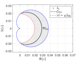
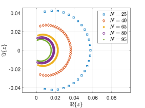
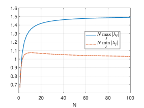
Figure 3.1. Eigenvalues of $\boldsymbol{M}$ in (3.6). Left: Distribution of $\lambda_{j}=\lambda_{N,j}$ with $N=51$ in the crescent-shaped region (left). Middle: Distributions of the eigenvalues with various $N$. Right: Behaviour of the eigenvalues with the smallest and largest magnitudes for $1\leq N\leq 100.$

In the above derivations, we chose the basis functions in (3.3)-(3.4) with proper coefficients so that the derivative matrix in the linear system (3.5) became an identity matrix, but as a matter of fact, the eigenvalues are independent of the choice of basis functions. More precisely, consider any two sets of bases:

$${}_{0}{\mathbb{P}_{N}}={\rm span}\big{\{}\psi_{k}\,:\,0\leq k\leq N-1\big{\}},\quad{}^{0}{\mathbb{P}_{N}}={\rm span}\big{\{}\psi_{k}^{*}\,:\,0\leq k\leq N-1\big{\}}.$$

Let $\boldsymbol{P},\boldsymbol{Q}$ be the corresponding transformation matrices such that

$$\psi_{k}(t)=\sum_{j=0}^{N-1}\boldsymbol{P}_{jk}\phi_{j}(t),\quad\psi_{k}^{*}(t)=\sum_{j=0}^{N-1}\boldsymbol{Q}_{kj}\phi_{j}^{*}(t).$$

Further, let $\widehat{\boldsymbol{S}},\widehat{\boldsymbol{M}}$ be the related derivative and mass matrices, that is, $\widehat{\boldsymbol{S}}_{jk}=(\psi_{k}^{\prime},\psi_{j}^{*})$ and $\widehat{\boldsymbol{M}}_{jk}=(\psi_{k},\psi_{j}^{*}).$ It can be shown by direct manipulations the following results, so we leave its proof to the interested readers.

Corollary 3.1.

The eigenvalues $\{\lambda_{j}:=\lambda_{N,j}\}_{j=1}^{N}$ of the matrix $\boldsymbol{M}$ in (3.6) are also the eigenvalues of the generalised eigenvalue problem:

$$\widehat{\boldsymbol{S}}\hat{\boldsymbol{v}}=\lambda\widehat{\boldsymbol{M}}\hat{\boldsymbol{v}},$$

where the corresponding eigenvectors are

$$\hat{\boldsymbol{v}}_{j}=\frac{(\boldsymbol{Q}\boldsymbol{P})^{-1}\boldsymbol{v}_{j}}{|(\boldsymbol{Q}\boldsymbol{P})^{-1}\boldsymbol{v}_{j}|},\quad 1\leq j\leq N,$$

with $\{\boldsymbol{v}_{j}\}_{j=1}^{N}$ being the eigenvectors of $\boldsymbol{M}$ given in (3.8).

3.2. Collocation scheme at Legendre points

Trefethen and Trummer [27] studied the collocation scheme for hyperbolic problems on the nodes consisting of $N$ Legendre-Gauss points and an endpoint (to impose the underlying one-sided boundary condition). In what follows, we employ this scheme to the model problem (3.1), and show that it can be reformulated into a Petrov-Galerkin scheme. We can then characterise the eigenvalues of the spectral differentiation matrix through zeros of the BP.

Let $t_{0}=-1$ and $t_{1}<t_{2}<\cdots<t_{N}$ be the Legendre-Gauss points, i.e., zeros of $P_{N}(t)$, and let $\{h_{j}\}_{j=0}^{N}\subseteq{\mathbb{P}}_{N}$ be the corresponding Lagrange interpolating basis polynomials such that $h_{j}(t_{i})=\delta_{ij}.$ The collocation scheme in [27] adapted to (3.1) is to find $u_{N}\in{\mathbb{P}_{N}}$ such that

$$u_{N}^{\prime}(t_{j})=\sigma u_{N}(t_{j}),\;\;1\leq j\leq N;\quad u_{N}(t_{0})=u_{0}.$$ (3.11)

Since ${}_{0}{\mathbb{P}_{N}}={\rm span}\{h_{j}:1\leq j\leq N\},$ we write and denote

$$u_{N}(t)=\sum_{j=0}^{N}u_{N}(t_{j})h_{j}(t),\quad\boldsymbol{u}=(u_{N}(t_{1}),\cdots,u_{N}(t_{N}))^{\top}.$$

Then we obtain the linear system

$$\big{(}\boldsymbol{D}-\sigma\boldsymbol{I}_{N}\big{)}\boldsymbol{u}=-u_{0}\boldsymbol{h}_{0}^{\prime},$$ (3.12)

where $\boldsymbol{h}_{0}^{\prime}=(h_{0}^{\prime}(t_{1}),\cdots,h_{0}^{\prime}(t_{N}))^{\top},$ and the spectral differentiation matrix $\boldsymbol{D}\in{\mathbb{R}}^{N\times N}$ with the entries ${\boldsymbol{D}}_{ij}=h_{j}^{\prime}(t_{i})$ for $1\leq i,j\leq N.$ One verifies readily that

$$h_{0}(t)=(-1)^{N}P_{N}(t),\quad h_{j}(t)=\frac{1+t}{1+t_{j}}l_{j}(t),\quad 1\leq j\leq N,$$

where $\{l_{j}(t)\}_{j=1}^{N}\subseteq{\mathbb{P}}_{N-1}$ are the Lagrange interpolating basis polynomials at the Legendre-Gauss points $\{t_{j}\}_{j=1}^{N}.$ Thus, we can compute the entries of $\boldsymbol{D}$ via

$${\boldsymbol{D}}_{ij}=h_{j}^{\prime}(t_{i})=\frac{1}{1+t_{j}}\delta_{ij}+\frac{1+t_{i}}{1+t_{j}}l_{j}^{\prime}(t_{i}),\quad 1\leq i,j\leq N,$$ (3.13)

where $\{l_{j}^{\prime}(t_{i})\}$ can be computed by the formulas in [20, Ch.​ 3].

To facilitate the eigenvalue analysis of $\boldsymbol{D}$, we reformulate (3.11) as a pseudospectral scheme. Let $\{\omega_{j}\}_{j=1}^{N}$ be the Legendre-Gauss quadrature weights corresponding to $\{t_{j}\}_{j=1}^{N},$ and denote the induced discrete inner product by $\langle\cdot,\cdot\rangle_{N}.$ Then we obtain from (3.11) that

$$\langle u_{N}^{\prime},\psi\rangle_{N}=\sigma\langle u_{N},\psi\rangle_{N},\;\;u_{N}(-1)=u_{0},\;\;\forall\psi\in{\mathbb{P}}_{N-1},$$ (3.14)

As the Legendre-Gauss quadrature rule has a degree of precision $2N-1,$ the scheme (3.14) is equivalent to the Petrov-Galerkin scheme: find $u_{N}=u_{0}+v_{N}\in{\mathbb{P}_{N}}$ with $v_{N}\in{{}_{0}\mathbb{P}_{N}}$ such that

$$(v_{N}^{\prime},\psi)-\sigma(v_{N},\psi)=\sigma(u_{0},\psi),\;\;\forall\psi\in{\mathbb{P}}_{N-1}.$$ (3.15)

It is essential to choose the basis functions for ${}_{0}{\mathbb{P}_{N}}$ as

$$\phi_{0}(t)=\frac{1}{\sqrt{2}}(t+1),\quad\phi_{k}(t)=\frac{1}{\sqrt{2}}(P_{k+1}(t)-P_{k-1}(t)),\quad 1\leq k\leq N-1,$$ (3.16)

and choose $\{\psi_{j}(t)=\frac{1}{\sqrt{2}}P_{j}(t)\}_{j=0}^{N-1}$ as the basis polynomials for the test function space. One verifies from (2.11) and (2.13)-(2.14) that $(\phi_{k}^{\prime},\psi_{j})=\delta_{jk}$ and

$$\hbox to0.0pt{\hskip 2.89581pt\leavevmode\hbox{\set@color$\overline{\hbox{}}$}\hss}{\leavevmode\hbox{\set@color$\boldsymbol{M}$}}_{jk}=(\phi_{k},\psi_{j})=\begin{dcases}1,&k=j=0,\\ -\frac{1}{2j+1},&k=j+1,\\ \frac{1}{2j+1},&k=j-1,\\ 0,&{\rm otherwise}.\end{dcases}$$ (3.17)

Then the system corresponding to (3.15) reads

$$\big{(}\boldsymbol{I}_{N}-\sigma\hbox to0.0pt{\hskip 2.89581pt\leavevmode\hbox{\set@color$\overline{\hbox{}}$}\hss}{\leavevmode\hbox{\set@color$\boldsymbol{M}$}}\big{)}\bar{\boldsymbol{v}}=\sqrt{2}\sigma u_{0}\boldsymbol{e}_{1},$$ (3.18)

where

$$v_{N}(t)=\sum_{k=0}^{N-1}\bar{v}_{k}\phi_{k}(t),\quad\bar{\boldsymbol{v}}=(\bar{v}_{0},\cdots,\bar{v}_{N-1})^{\top}.$$

Lemma 3.1.

The spectral differentiation matrix $\boldsymbol{D}$ in (3.12) is similar to the inverse $\hbox to0.0pt{\hskip 2.89581pt\leavevmode\hbox{\set@color$\overline{\hbox{}}$}\hss}{\leavevmode\hbox{\set@color$\boldsymbol{M}$}}^{-1},$ i.e.,

$$\boldsymbol{D}=\boldsymbol{\Phi}\,\hbox to0.0pt{\hskip 2.89581pt\leavevmode\hbox{\set@color$\overline{\hbox{}}$}\hss}{\leavevmode\hbox{\set@color$\boldsymbol{M}$}}^{-1}\,\boldsymbol{\Phi}^{-1},$$

where $\boldsymbol{\Phi}\in{\mathbb{R}}^{N\times N}$ has the entries $\{\boldsymbol{\Phi}_{ik}=\phi_{k}(t_{i})\}_{1\leq i\leq N}^{0\leq k\leq N-1}$ and the basis $\{\phi_{k}\}$ is given in (3.16).

Proof.

We first show that

$$\boldsymbol{D}\boldsymbol{\Phi}=\boldsymbol{\Phi}^{\prime},\quad\boldsymbol{\Phi}^{\prime}_{ik}=\phi_{k}^{\prime}(t_{i}).$$ (3.19)

For any $p\in{}_{0}{\mathbb{P}_{N}},$ we have the exact differentiation

$$p^{\prime}(t)=\sum_{j=1}^{N}p(t_{j})h_{j}^{\prime}(t),\;\;\;{\rm so}\;\;\;\boldsymbol{p}^{\prime}=\boldsymbol{D}\boldsymbol{p},$$

where $\boldsymbol{p}=(p(t_{1}),\cdots,p(t_{N}))^{\top}$ and $\boldsymbol{p}^{\prime}=(p^{\prime}(t_{1}),\cdots,p^{\prime}(t_{N}))^{\top}.$ Taking $p$ to be columns of $\boldsymbol{\Phi},$ yields

$$\boldsymbol{\Phi}^{\prime}=(\boldsymbol{\phi}_{0}^{\prime},\cdots,\boldsymbol{\phi}_{N-1}^{\prime})=\boldsymbol{D}(\boldsymbol{\phi}_{0},\cdots,\boldsymbol{\phi}_{N-1})=\boldsymbol{D}\boldsymbol{\Phi}.$$

We now introduce the matrix related to the dual basis functions: $\boldsymbol{\Psi}\in\mathbb{R}^{N\times N}$ with $\boldsymbol{\Psi}_{jk}=\psi_{j}(t_{k})\omega_{k}$. One verified readily from (3.14) that

$$(\boldsymbol{\Psi}\boldsymbol{\Phi})_{jk}=\sum_{l=0}^{N-1}\boldsymbol{\Psi}_{jl}\boldsymbol{\Phi}_{lk}=\sum_{l=0}^{N-1}\psi_{j}(t_{l})\phi_{k}(t_{l})\omega_{l}=\langle\phi_{k},\psi_{j}\rangle_{N}=(\phi_{k},\psi_{j})=\hbox to0.0pt{\hskip 2.89581pt\leavevmode\hbox{\set@color$\overline{\hbox{}}$}\hss}{\leavevmode\hbox{\set@color$\boldsymbol{M}$}}_{jk},$$

and

$$(\boldsymbol{\Psi}\boldsymbol{\Phi}^{\prime})_{jk}=\langle\phi_{k}^{\prime},\psi_{j}\rangle_{N}=(\phi_{k}^{\prime},\psi_{j})=\delta_{jk},$$

so we have

$$\boldsymbol{\Psi}\boldsymbol{\Phi}=\hbox to0.0pt{\hskip 2.89581pt\leavevmode\hbox{\set@color$\overline{\hbox{}}$}\hss}{\leavevmode\hbox{\set@color$\boldsymbol{M}$}},\quad\boldsymbol{\Psi}\boldsymbol{\Phi}^{\prime}=\boldsymbol{I}_{N}.$$ (3.20)

Then from (3.19)-(3.20), we obtain immediately that

$$\boldsymbol{D}=\boldsymbol{\Phi}^{\prime}\,\boldsymbol{\Phi}^{-1}=\boldsymbol{\Psi}^{-1}\,\boldsymbol{\Phi}^{-1}=\boldsymbol{\Phi}\,\hbox to0.0pt{\hskip 2.89581pt\leavevmode\hbox{\set@color$\overline{\hbox{}}$}\hss}{\leavevmode\hbox{\set@color$\boldsymbol{M}$}}^{-1}\,\boldsymbol{\Phi}^{-1}.$$

This ends the proof. ∎

Remarkably, we can show that the eigenvalues of the matrix  $\overline{\hbox{}}$$\boldsymbol{M}$ are zeros of the classical BP, which together with Lemma 3.1 allows us to characterise the distribution of eigenvalues of $\boldsymbol{D}$.

Theorem 3.2.

Let $\{\bar{\lambda}_{j}:=\bar{\lambda}_{N,j}\}_{j=1}^{N}$ be the eigenvalues of the matrix  $\overline{\hbox{}}$$\boldsymbol{M}$ with $N\geq 2.$

• The eigenvalues $\{\bar{\lambda}_{j}=-z_{j}\}_{j=1}^{N}$ with $\big{\{}z_{j}:=z_{N,j}\big{\}}$ being zeros of the Bessel polynomial $B_{N}(x)$ defined in (2.7), so the eigenvalues are all simple and conjugate of each other. For odd $N,$ its unique real eigenvalue behaves like $-Z_{N,2}$ in (2.10).

• All the eigenvalues are in the open right half-plane and located in crescent-shaped region:

  $$\bar{\lambda}_{j}\in\mathcal{R}_{N}^{+}:=\left\{z=\rho{\rm e}^{{\rm i}\theta}\in\mathbb{C}:\frac{1}{N+2/3}<\rho\leq\frac{1+\cos\theta}{N+1},\;\;|\theta|<\pi-\Theta_{N,2}\right\},$$

  for $1\leq j\leq N$, where $\Theta_{N,2}$ is given in (2.9) and the equal sign can be only attainable at $\theta=0.$

The corresponding eigenvector are

$$\boldsymbol{\bar{v}}_{j}=\frac{\boldsymbol{\bar{b}}_{j}}{|\boldsymbol{\bar{b}}_{j}|},\quad\boldsymbol{\bar{b}}_{j}=\big{(}B_{0}(-\bar{\lambda}_{j}),B_{1}(-\bar{\lambda}_{j}),\cdots,B_{N-1}(-\bar{\lambda}_{j})\big{)}^{\top},\quad 1\leq j\leq N.$$ (3.21)

Proof.

We rewrite the three-term recurrence relation (2.3) as

$$\begin{dcases}-zB_{0}(z)=B_{0}(z)-B_{1}(z),\\ -zB_{j}(z)=\frac{1}{2j+1}B_{j-1}(z)-\frac{1}{2j+1}B_{j+1}(z),\;\;\;1\leq j\leq N-1,\end{dcases}$$ (3.22)

and denote

$$\bar{\boldsymbol{b}}(z):=(B_{0}(z),B_{1}(z),\cdots,B_{N-1}(z))^{\top},\quad\boldsymbol{e}_{N}:=(0,\cdots,0,1)^{\top}\in{\mathbb{R}}^{N}.$$

In view of (3.17), we can reformulate (3.22) as the matrix form

$$-z\boldsymbol{\bar{b}}(z)=\hbox to0.0pt{\hskip 2.89581pt\leavevmode\hbox{\set@color$\overline{\hbox{}}$}\hss}{\leavevmode\hbox{\set@color$\boldsymbol{M}$}}\boldsymbol{\bar{b}}(z)-\frac{1}{2N-1}B_{N}^{(2)}(z)\boldsymbol{e}_{N}.$$ (3.23)

Taking $z=z_{j}=-\bar{\lambda}_{j}$ in (3.23), we obtain immediately that $\bar{\lambda}_{j}\boldsymbol{v}_{j}=\hbox to0.0pt{\hskip 2.89581pt\leavevmode\hbox{\set@color$\overline{\hbox{}}$}\hss}{\leavevmode\hbox{\set@color$\boldsymbol{M}$}}\boldsymbol{v}_{j}$ for $1\leq j\leq N$ with the corresponding eigenvectors $\{\boldsymbol{\bar{b}}_{j}:=\boldsymbol{\bar{b}}(-\bar{\lambda}_{j})\}$ given in (3.21). With this, we claim these properties from Theorem 2.1 and Remark 2.1 with $\alpha=2$. ∎

In Figure 3.2 (left), we plot the region $\mathcal{R}_{N}^{+}$ with $N=51$ confined by the cardioid curve:

$$\mathcal{C}_{N}^{+}=\Big{\{}z=\rho{\rm e}^{{\rm i}\theta}\in\mathbb{C}:\rho=\frac{1+\cos\theta}{N+1},\;\;-\pi<\theta\leq\pi\Big{\}},$$

and the semi-circle: $|z|={1}/(N+2/3)$ with $\theta\in[-\pi/2,\pi/2].$ Like Figure 3.1, we also illustrate the distributions of the eigenvalues for various $N,$ and examine the behaviour of the eigenvalues with the smallest and largest magnitudes, from which we observe similar asymptotic properties.

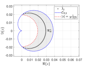
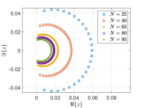
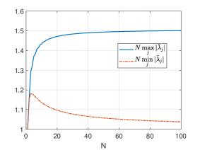
Figure 3.2. Eigenvalues of  $\overline{\hbox{}}$$\boldsymbol{M}$ in (3.17). Left: Distribution of $\bar{\lambda}_{j}=\bar{\lambda}_{N,j}$ with $N=51$ in the crescent-shaped region. Middle: Distributions of the eigenvalues for different $N$. Right: Behaviour of the eigenvalues with the smallest and largest magnitudes for $1\leq N\leq 100$.

As a direct consequence of Lemma 3.1 and Theorem 3.2, we have the following important result on the eigenvalues and eigenvectors of $\boldsymbol{D}.$

Corollary 3.2.

The eigenvalues $\{\lambda_{j}^{D}\}_{j=1}^{N}$ of $\boldsymbol{D}$ in (3.12)-(3.13) are reciprocal of the eigenvalues $\{\bar{\lambda}_{j}\}_{j=1}^{N}$ of  $\overline{\hbox{}}$$\boldsymbol{M}$ in (3.17)-(3.18), so they are distinct, and conjugate of each other, except for one real eigenvalue when $N$ is odd. Moreover, all the eigenvalues satisfy $\Re\{\lambda_{j}^{D}\}>0,$ and lie in the region

$$\widehat{{\mathcal{R}}}_{N}^{+}:=\Big{\{}z=\rho e^{{\rm i}\theta}\in\mathbb{C}:\frac{N+1}{1+\cos\theta}\leq\rho<N+\frac{2}{3},\,\,|\theta|<\pi-\Theta_{N,2}\Big{\}},\quad 1\leq j\leq N.$$ (3.24)

The corresponding eigenvector of $\lambda_{j}^{D}$ is

$$\boldsymbol{v}_{j}^{D}=\frac{\boldsymbol{b}_{j}^{D}}{|\boldsymbol{b}_{j}^{D}|},\quad\boldsymbol{b}_{j}^{D}=\boldsymbol{\Phi}\boldsymbol{\bar{b}}_{j},\quad 1\leq j\leq N,$$

where the matrix $\boldsymbol{\Phi}$ is given in Lemma 3.1 and $\{\boldsymbol{\bar{b}}_{j}\}$ is given by (3.21).

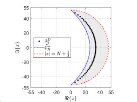
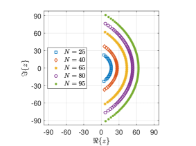
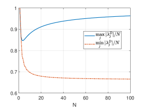
Figure 3.3. Eigenvalues of $\boldsymbol{D}$ in (3.12) with the same setting as Figure 3.2. Here $\widehat{\mathcal{C}}_{N}^{+}$ denotes the left boundary curve in (3.24).

Remark 3.1.

The Bessel polynomial directly bears on the modified Bessel function (cf. [9]):

$$B_{N}(z)=\sqrt{\frac{2}{\pi z}}{\rm e}^{1/z}K_{N+\frac{1}{2}}(1/z),$$

which agrees with the identification in [28]. However, we can also identify the eigenvectors through our approach.

We illustrate in Figure 3.3 the eigenvalues of $\boldsymbol{D}$ in the same setting as in Figure 3.2. It is seen from (3.24) that $|\lambda_{j}^{D}|=O(N).$ Indeed, by Remark 2.1, the unique real eigenvalue for odd $N$ behaves like

$$\lambda_{(N+1)/2}^{D}=\frac{N}{\nu}+O(1),\;\;\;\nu\approx 1.50888.$$

4. Eigenvalue analysis of LDPG methods for second-order IVPs

In this section, we extend the eigenvalue analysis to the second-order IVP:

$$u^{\prime\prime}(t)=\sigma u(t),\;\;\;t\in I;\quad u(-1)=u_{0},\quad u^{\prime}(-1)=u_{1},\quad$$ (4.1)

where the constants $\sigma\neq 0,$ and $u_{0},u_{1}$ are given. Introduce the dual approximation spaces

$$V_{N}=\big{\{}\phi\in\mathbb{P}_{N+1}:\phi(-1)=\phi^{\prime}(-1)=0\big{\}},\quad V_{N}^{*}=\big{\{}\psi\in\mathbb{P}_{N+1}:\psi(1)=\psi^{\prime}(1)=0\big{\}}.$$

Here, we set the highest degree to be $N+1$ so that ${\rm dim}(V_{N})={\rm dim}(V_{N}^{*})=N.$ Let $\{t_{i},\omega_{i}\}_{i=0}^{N+1}$ be the Legendre-Gauss-Lobatto quadrature nodes and weights with the discrete inner product and the exactness of quadrature

$$\langle f,g\rangle_{N}:=\sum_{i=0}^{N+1}f(t_{i})g(t_{i})\omega_{i};\quad\langle f,g\rangle_{N}=(f,g),\quad\forall\,f\cdot g\in{\mathbb{P}}_{2N+1}.$$ (4.2)

The Legendre pseudospectral dual-Petrov-Galerkin scheme for (4.1) is to find $u_{N}=u_{0}+(1+t)u_{1}+v_{N}\in\mathbb{P}_{N+1}$ with $v_{N}\in V_{N}$ such that

$$\langle v_{N}^{\prime},\psi^{\prime}\rangle_{N}+\sigma\langle v_{N},\psi\rangle_{N}=-\sigma\langle u_{0}+(1+t)u_{1},\psi\rangle_{N},\quad\forall\,\psi\in V_{N}^{*}.$$ (4.3)

Choose the basis functions for $V_{N}$ and $V_{N}^{*}$ as

$$\begin{split}\phi_{k}(t)&=c_{k}\big{(}P_{k}(t)+a_{k}P_{k+1}(t)+b_{k}P_{k+2}(t)\big{)}\in V_{N},\\ \phi_{k}^{*}(t)&=d_{k}\big{(}P_{k}(t)-a_{k}P_{k+1}(t)+b_{k}P_{k+2}(t)\big{)}\in V_{N}^{*},\end{split}$$

for $0\leq k\leq N-1,$ where

$$a_{k}=\frac{2k+3}{k+2},\quad b_{k}=\frac{k+1}{k+2},\quad c_{k}=\frac{k+2}{\sqrt{2}},\quad d_{k}=\frac{1}{\sqrt{2}(k+1)(2k+3)}.$$

Write and denote

$$v_{N}(t)=\sum_{k=0}^{N-1}\tilde{v}_{k}\phi_{k}(t),\quad\tilde{\boldsymbol{v}}=(\tilde{v}_{0},\cdots,\tilde{v}_{N-1})^{\top}.$$

The matrix form of (4.3) reads

$$\big{(}\boldsymbol{I}_{\!N}-\sigma\boldsymbol{{M}}^{(2)}\big{)}\tilde{\boldsymbol{v}}=\sigma\boldsymbol{g},\;\;{\rm where}\;\;\boldsymbol{g}:=\frac{2u_{0}+u_{1}}{3\sqrt{2}}\boldsymbol{e}_{1}+\frac{u_{1}}{15\sqrt{2}}\boldsymbol{e}_{2}.$$ (4.4)

Thanks to (4.2), we verify from the properties (2.11)-(2.12) readily that

$$\langle\phi_{k}^{\prime\prime},\phi_{j}^{*}\rangle_{N}=(\phi_{k}^{\prime\prime},\phi_{j}^{*})=\delta_{jk},\quad 0\leq j,k\leq N-1,$$

and the mass matrix $\boldsymbol{{M}}^{(2)}\in\mathbb{R}^{N\times N}$ is a penta-diagonal (non-symmetric) matrix with nonzero entries given by

$$\boldsymbol{M}_{jk}^{(2)}=\langle\phi_{k},\phi_{j}^{*}\rangle_{N}=\begin{dcases}\frac{2(j-1)}{j(2j+1)}d_{j}c_{j-2},&k=j-2,\;\;2\leq j\leq N-1,\\ \frac{4}{(j+1)(j+2)}d_{j}c_{j-1},&k=j-1,\;\;1\leq j\leq N-1,\\ \Big{(}\frac{2}{2j+1}-\frac{2(2j+3)}{(j+2)^{2}}+\Big{(}\frac{j+1}{j+2}\Big{)}^{2}\frac{2}{2j+5}\Big{)}d_{j}c_{j},&k=j,\;\;0\leq j\leq N-2,\\ \frac{-N^{3}-2N^{2}+4N+2}{N(N+1)^{2}(2N-1)(2N+1)},&k=j=N-1,\\ -\frac{4}{(j+2)(j+3)}d_{j}c_{j+1},&k=j+1,\;\;0\leq j\leq N-2,\\ \frac{2(j+1)}{(j+2)(2j+5)}d_{j}c_{j+2},&k=j+2,\;\;0\leq j\leq N-3.\end{dcases}$$ (4.5)

Note that for $j=k=N-1$, the LGL quadrature is not exact, so we obtain this entry via

$$\begin{split}\langle\phi_{N-1},&\phi_{N-1}^{*}\rangle_{N}=c_{N-1}d_{N-1}\big{\{}\|P_{N-1}\|^{2}-a_{N-1}^{2}\|P_{N}\|^{2}+b_{N-1}^{2}\langle P_{N+1},P_{N+1}\rangle_{N}\big{\}}\\ &=\frac{N+1}{N(2N-1)(2N+1)}-\frac{1}{N(N+1)}+\frac{N}{2(N+1)(2N+1)}\langle P_{N+1},P_{N+1}\rangle_{N}\\ &=\frac{-N^{3}-2N^{2}+4N+2}{N(N+1)^{2}(2N-1)(2N+1)},\end{split}$$ (4.6)

where we used the property (see [20, p.​ 101]):

$$\langle P_{N+1},P_{N+1}\rangle_{N}=\frac{2}{N+1}.$$

Remarkably, we can exactly characterise the eigenvalues of $\boldsymbol{M}^{(2)}$ as follows.

Theorem 4.1.

There holds the relation

$$\boldsymbol{M}^{(2)}=\widetilde{\boldsymbol{M}}\times\widetilde{\boldsymbol{M}},$$ (4.7)

where $\widetilde{\boldsymbol{M}}$ is the Jacobi matrix of the three-term recurrence relation of the GBPs $\{B_{n}^{(4)}(z)\},$ i.e., (2.3) with $\alpha=4,\beta=2.$ Consequently, the eigenvalues of $\boldsymbol{{M}}^{(2)}$ are

$$\mu_{j}=\big{(}z_{j}^{(4)}\big{)}^{2},\quad 1\leq j\leq N,$$

where $\{z_{j}^{(4)}\}$ are zeros of the GBP $B_{N}^{(4)}(z).$ They are simple, conjugate of each other and lie in the region

$$\mu_{j}\in\mathcal{R}_{N,4}^{(2)}:=\Big{\{}z=\rho{\rm e}^{{\rm i}\theta}\in\mathbb{C}:\frac{1}{(N+\frac{5}{3})^{2}}<\rho\leq\Big{(}\frac{1+\cos(\theta/2)}{N+3}\Big{)}^{2},\;\;|\theta|\leq 2(\pi-\Theta_{N,4})\Big{\}},$$ (4.8)

for $1\leq j\leq N,$ where $\Theta_{N,4}$ is given in (2.9) and the equal sign can be only attained at $\theta=0.$ Furthermore, the corresponding eigenvectors are

$$\tilde{\boldsymbol{v}}_{j}=\frac{\tilde{\boldsymbol{b}}_{j}}{|\tilde{\boldsymbol{b}}_{j}|},\quad\tilde{\boldsymbol{b}}_{j}:=\big{(}B_{0}^{(4)}(z_{j}^{(4)}),B_{1}^{(4)}(z_{j}^{(4)}),\cdots,B_{N-1}^{(4)}(z_{j}^{(4)})\big{)}^{\top},\quad 1\leq j\leq N.$$ (4.9)

Proof.

We write the recurrence relation (2.3) with $\alpha=4,\beta=2$ and $j=0,\cdots,N-2$ as the matrix form

$$-z\tilde{\boldsymbol{b}}(z)=\widetilde{\boldsymbol{M}}\tilde{\boldsymbol{b}}(z)-\frac{N+2}{(N+1)(2N+1)}B_{N}^{(4)}(z)\boldsymbol{e}_{N},$$ (4.10)

where $\tilde{\boldsymbol{b}}(z)=\big{(}B_{0}^{(4)}(z),B_{1}^{(4)}(z),\cdots,B_{N-1}^{(4)}(z)\big{)}^{\top}$ and $\widetilde{\boldsymbol{M}}$ is the tri-diagonal Jacobi matrix with nonzero entries given by

$$\widetilde{\boldsymbol{M}}_{jk}=\begin{dcases}\frac{j}{(j+1)(2j+3)},&k=j-1,\;\;\;1\leq j\leq N-1,\\ \frac{1}{j+1}-\frac{1}{j+2},&k=j,\;\;0\leq j\leq N-1,\\ -\frac{j+3}{(j+2)(2j+3)},&k=j+1,\;\;0\leq j\leq N-2.\end{dcases}$$ (4.11)

We conclude from (4.10) that the eigenvalues of $\widetilde{\boldsymbol{M}}$ are $N$ zeros of $B_{N}^{(4)}(z)$ with the corresponding unit eigenvectors given by (4.9).

Notably, we can directly verify from (4.5) and (4.11) that $\boldsymbol{M}^{(2)}=\widetilde{\boldsymbol{M}}\times\widetilde{\boldsymbol{M}}.$ In view of Theorem 2.1 with $\alpha=4$, we complete the proof. ∎

In Figure 4.1 (left), we depict the distribution of eigenvalues of $\boldsymbol{M}^{(2)}$ and the region $\mathcal{R}_{N,4}^{(2)}$ given in (4.8) with $N=51$. Apparently, they are all distributed within the shaded region as shown in Theorem 4.1. We also demonstrate the eigenvalues for various $N,$ and illustrate behaviours of the maximum and the minimum magnitudes in the other two sub-figures in Figure 4.1. As predicted by Theorem 4.1, we have $|\mu_{j}|=O(N^{-2}).$

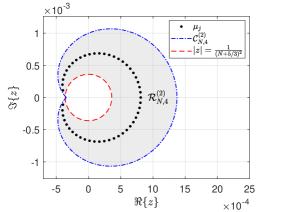
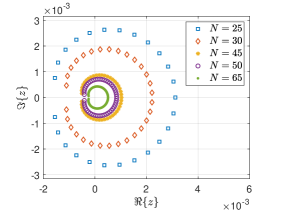
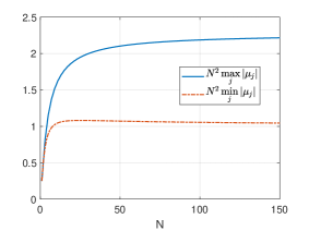
Figure 4.1. Eigenvalues of $\boldsymbol{M}^{(2)}$ in (4.5) with the same setting as Figure 3.2.

It is seen from the above discussions that with the appropriate choice of basis functions, we were able to associate the mass matrix of the pseudospectral scheme (4.3) with the GBP through (4.7). However, for the spectral Petrov-Galerkin scheme, the eigenvalues in magnitude appear an $O(N^{-3})$ perturbation of those for the pseudospectral ones. To demonstrate this, we replace the discrete inner product in (4.3) by the continuous inner product, leading to the spectral dual-Petrov-Galerkin scheme for (4.1): find $u_{N}=u_{0}+(1+t)u_{1}+v_{N}\in\mathbb{P}_{N+1}$ with $v_{N}\in V_{N}$ such that

$$(v_{N}^{\prime},\psi^{\prime})+\sigma(v_{N},\psi)=-\sigma(u_{0}+(1+t)u_{1},\psi),\quad\forall\psi\in V_{N}^{*}.$$ (4.12)

The only difference is to modify the last entry of $\boldsymbol{M}^{(2)}$ in the linear system (4.4), i.e., (4.6) by

$$(\phi_{N-1},\phi_{N-1}^{*})=-\frac{2(N^{2}+N-3)}{N(N+1)(2N-1)(2N+3)}=\langle\phi_{N-1},\phi_{N-1}^{*}\rangle_{N}+O(N^{-2}).$$

Numerically, we find from Figure 4.2 that the eigenvalues $\{\tilde{\mu}_{j}\}$ of the modified matrix are a $O(N^{-3})$ perturbation of the eigenvalues $\{\mu_{j}\}$ of $\boldsymbol{M}^{(2)}$.

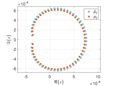
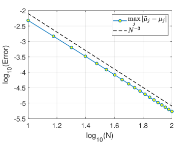
Figure 4.2. Eigenvalues of $\boldsymbol{M}^{(2)}$ in the pseudospectral scheme (4.3) and the spectral scheme (4.12). Left: Distributions with $N=54.$ Right: Asymptotic order $O(N^{-3})$.

5. Eigenvalue analysis of LDPG methods for higher-order IVPs

In this section, we extend the eigenvalue analysis to higher-order IVPs with a focus on the third-order IVPs. We also consider the reformulation of the high-order IVPs as a system of first-order equations for which we can precisely characterise the eigenvalues.

5.1. Third-order IVPs

To fix the idea, we consider the third-order IVP:

$$u^{\prime\prime\prime}(t)=\sigma u(t),\quad t\in I;\;\quad u(-1)=u_{0},\;\;u^{\prime}(-1)=u_{1},\;\;u^{\prime\prime}(-1)=u_{2},$$ (5.1)

where $\sigma\not=0,u_{0},u_{1}$ and $u_{2}$ are given constants.

Define the dual approximation spaces

$$\begin{split}&V_{N}=\{\phi\in\mathbb{P}_{N+2}:\phi(-1)=\phi^{\prime}(-1)=\phi^{\prime\prime}(-1)=0\},\\ &V_{N}^{*}=\{\phi\in\mathbb{P}_{N+2}:\phi(1)=\phi^{\prime}(1)=\phi^{\prime\prime}(1)=0\},\end{split}$$

with ${\rm dim}(V_{N})={\rm dim}(V_{N}^{*})=N.$ Then the LDPG scheme for (5.1) is

$$\begin{dcases}\text{Find}\;u_{N}=u_{0}+(1+t)u_{1}+\frac{1}{2}(1+t)^{2}u_{2}+v_{N}\in\mathbb{P}_{N+2}\;\;\text{with}\;\;v_{N}\in V_{N}\;\;\text{s.t.}\\ (v_{N}^{\prime},\psi^{\prime\prime})-\sigma(v_{N},\psi)=\sigma(u_{0}+u_{1}(1+t)+\frac{u_{2}}{2}(1+t)^{2},\psi),\quad\forall\psi\in V_{N}^{*}.\end{dcases}$$ (5.2)

Choose the basis functions

$$\begin{split}\phi_{k}(t)&=d_{k}\big{(}P_{k}(t)+a_{k}P_{k+1}(t)+b_{k}P_{k+2}(t)+c_{k}P_{k+3}(t)\big{)}\in V_{N},\\ \phi_{k}^{*}(t)&=e_{k}\big{(}P_{k}(t)-a_{k}P_{k+1}(t)+b_{k}P_{k+2}(t)-c_{k}P_{k+3}(t)\big{)}\in V_{N}^{*},\end{split}$$

for $0\leq k\leq N-1$, where

$$a_{k}=\frac{3(2k+3)}{2k+5},\quad b_{k}=\frac{3(k+1)}{k+3},\quad c_{k}=\frac{(k+1)(2k+3)}{(k+3)(2k+5)},$$

$$d_{k}=\frac{(k+2)(k+3)}{2(2k+3)},\quad e_{k}=\frac{1}{(k+1)(k+2)(2k+3)}.$$

Then we can write and denote

$$v_{N}(t)=\sum_{k=0}^{N-1}\tilde{v}_{k}\phi_{k}(t),\quad\tilde{\boldsymbol{v}}=(\tilde{v}_{0},\cdots,\tilde{v}_{N-1})^{\top}.$$

Substituting $v_{N}$ into (5.2) and taking $\psi=\phi_{j}^{*}$ for $0\leq j\leq N-1$ lead to

$$(\boldsymbol{I}_{N}-\sigma\boldsymbol{M}^{(3)})\tilde{\boldsymbol{v}}=\sigma\boldsymbol{g},$$ (5.3)

where the elements of the column-$N$ vector $\boldsymbol{g}$ is given by

$$\boldsymbol{g}_{j}=(u_{0}+u_{1}(1+t)+\frac{u_{2}}{2}(1+t)^{2},\phi_{j}^{*}),\quad 0\leq j\leq N-1.$$

Using the properties of Legendre polynomials, we find that the nonzero entries of the seven-diagonal (non-symmetric) matrix $\boldsymbol{M}^{(3)}$ are given by

$$\begin{split}\boldsymbol{M}_{jk}^{(3)}=(\phi_{k},\phi_{j}^{*})=\begin{dcases}e_{j}d_{j-3}c_{j-3}\gamma_{j},&k=j-3,\\ e_{j}d_{j-2}\big{(}b_{j-2}\gamma_{j}-c_{j-2}a_{j}\gamma_{j+1}\big{)},&k=j-2,\\ e_{j}d_{j-1}\big{(}a_{j-1}\gamma_{j}-b_{j-1}a_{j}\gamma_{j+1}+c_{j-1}b_{j}\gamma_{j+2}\big{)}&k=j-1,\\ e_{j}d_{j}\big{(}\gamma_{j}-a_{j}^{2}\gamma_{j+1}+b_{j}^{2}\gamma_{j+2}-c_{j}^{2}\gamma_{j+3}\big{)},&k=j,\\ e_{j}d_{j+1}\big{(}-a_{j}\gamma_{j+1}+a_{j+1}b_{j}\gamma_{j+2}-b_{j+1}c_{j}\gamma_{j+3}\big{)},&k=j+1,\\ e_{j}d_{j+2}\big{(}b_{j}\gamma_{j+2}-a_{j+2}c_{j}\gamma_{j+3}\big{)},&k=j+2,\\ -e_{j}d_{j+3}c_{j}\gamma_{j+3},&k=j+3,\end{dcases}\end{split}$$

where $\gamma_{j}=2/(2j+1)$ as in (2.11), and the matrix of the third derivative is an identity matrix as

$$(\phi_{k}^{\prime\prime\prime},\phi_{j}^{*})=-(\phi_{k}^{\prime\prime},(\phi_{j}^{*})^{\prime})=(\phi_{k}^{\prime},(\phi_{j}^{*})^{\prime\prime})=\delta_{jk}.$$

We can directly verify the following properties and omit the details.

Proposition 5.1.

The matrix $\boldsymbol{M}^{(3)}$ is only different from $(\breve{\boldsymbol{M}})^{3}$ in three entries:

$$(j,k)=(N-2,N-1),\;(N-1,N-2),\;(N-1,N-1),$$ (5.4)

where $\breve{\boldsymbol{M}}$ is the tri-diagonal Jacobi matrix of the three-term recurrence relation for the GBPs $\{B_{n}^{(5)}(z)\}$ with nonzero entries given by

$$\breve{\boldsymbol{M}}_{jk}=\begin{dcases}\frac{j}{(j+2)(2j+3)},&k=j-1,\;\;\;1\leq j\leq N-1,\\ \frac{6}{(2j+3)(2j+5)},&k=j,\;\;0\leq j\leq N-1,\\ -\frac{j+4}{(j+2)(2j+5)},&k=j+1,\;\;0\leq j\leq N-2.\end{dcases}$$

Moreover, for these $(j,k)$ in (5.4),

$$|{\boldsymbol{M}}^{(3)}_{jk}-\big{(}\breve{\boldsymbol{M}}^{3}\big{)}_{jk}|=O(N^{-3}).$$

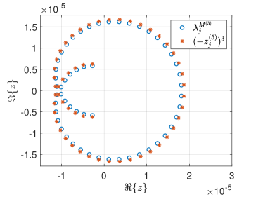
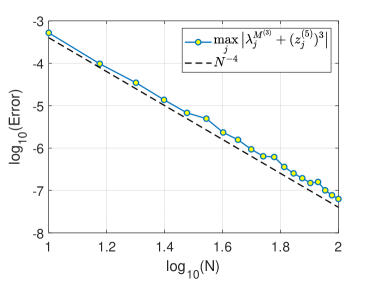
Figure 5.1. Left: Distributions of the eigenvalues of $\boldsymbol{M}^{(3)}$ and the cubic power of the Jacobi matrix of the GBPs $\{B_{n}^{(5)}\}$ with $N=54.$ Right: Numerical verification of (5.5).

Note that in Theorem 4.1, the matrix of the pseudospectral scheme (4.3) corresponds exactly to the Jacobi matrix of the GBPs $\{B_{n}^{(4)}(z)\}$. However, in the third-order case, it seems not possible to construct a pseudospectral scheme built upon a suitable quadrature rule so that $\boldsymbol{M}^{(3)}=(\breve{\boldsymbol{M}})^{3}.$ The numerical evidence in Figure 5.1 indicates

$$\max_{j}\big{|}\lambda_{j}^{\boldsymbol{M}^{(3)}}-(-z_{j}^{(5)})^{3}\big{|}=O(N^{-4}),$$ (5.5)

where $\{z_{j}^{(5)}\}_{j=1}^{N}$ are zeros of the GBP: $B_{N}^{(5)}(z).$

5.2. General $m$th-order IVPs

In general, we consider the $m$th-order IVP:

$$u^{(m)}(t)=\sigma u(t),\quad t\in I;\;\quad u^{(l)}(-1)=u_{l},\;\;\;l=0,\cdots,m-1,$$ (5.6)

where $\sigma\not=0$ and $\{u_{l}\}$ are given constants. Interestingly, we observe from the previous analysis of the LDPG method for (5.6) with $m=1,2,3$ the following pattern:

• As shown in Theorem 3.1 for the first-order IVP, the eigenvalues of the mass matrix can be exactly characterised by zeros of the GBP: $B_{N}^{(3)}(z).$

• For the second-order IVP, the eigen-pairs of the matrix for the pseudospectral scheme (4.3) can be exactly characterised by (square of) zeros of the GBP: $B_{N}^{(4)}(z)$ (see Theorem 4.1). However, the corresponding matrix of the spectral scheme differs from that of the pseudospectral version in the last entry (i.e., $j=k=N-1$), which leads to a perturbation in the eigenvalues of order $O(N^{-3})$ (from numerical evidences).

• For the third-order IVP, the mass matrix of the spectral dual-Petrov-Galerkin scheme differs from the cube of the Jacobi matrix corresponding to the GBPs: $B_{j}^{(5)}(z)$ in the last three entries, where the perturbation is of order $O(N^{-3}),$ see Proposition 5.1. However, a dual pseudospectral version with the exact correspondence to zeros of $B_{N}^{(5)}(z)$ might not exist.

For the general $m$-th order IVP (5.6), it is natural to speculate that the eigenvalues of the mass matrix be associated with the GBP: $B_{N}^{(m+2)}(z).$ More specifically, define the dual approximation spaces

$$\begin{split}&V_{N}=\big{\{}\phi\in\mathbb{P}_{N+m-1}:\phi^{(l)}(-1)=0,\;\;l=0,\cdots,m-1\big{\}},\\ &V_{N}^{*}=\big{\{}\psi\in\mathbb{P}_{N+m-1}:\psi^{(l)}(1)=0,\;\;l=0,\cdots,m-1\big{\}},\end{split}$$

with ${\rm dim}(V_{N})={\rm dim}(V_{N}^{*})=N.$ Then, as in the previous cases, we choose suitable compact combinations of Legendre polynomials as basis functions denoted by $\{\phi_{k},\phi_{k}^{*}\}_{k=0}^{N-1},$ respectively, such that $(\phi_{k}^{(m)},\phi_{j}^{*})=\delta_{jk}.$ Denote the $N$-by-$N$ mass matrix by $\boldsymbol{M}^{(m)}$ with entries $\boldsymbol{M}^{(m)}_{jk}=(\phi_{k},\phi_{j}^{*}).$ We conjecture that for $m<N,$ the matrix $\boldsymbol{M}^{(m)}$ differs from $(\breve{\boldsymbol{M}})^{m}$ in $2m-3$ entries, where $\breve{\boldsymbol{M}}$ is the tri-diagonal Jacobi matrix corresponding to the GBPs: $B_{j}^{(m+2)}(z).$ Moreover, we speculate that

$$\|\boldsymbol{M}^{(m)}-(\breve{\boldsymbol{M}})^{m}\|_{\infty}=O(N^{-m}),\quad\max_{1\leq j\leq N}\big{|}\lambda_{j}^{\boldsymbol{M}^{(m)}}-\big{(}\!\!-z_{j}^{(m+2)}\big{)}^{m}\big{|}=O(N^{-(m+1)}),$$

where $\{z_{j}^{(m+2)}\}$ are zeros of $B_{N}^{(m+2)}(z).$

5.3. LDPG method for $m$th-order IVP based on first-order system

Remarkably, we can show that if we rewrite the underlying IVP as a system of first-order equations, then we are able to exactly characterise the eigenvalues through zeros of the GBP: $B_{N}^{(3)}(z).$

To fix the idea, we still consider the third-order IVP (5.1), and reformulate it as the system

$$\begin{dcases}v_{0}^{\prime}(t)=v_{1}(t),\;\;v_{1}^{\prime}(t)=v_{2}(t),\;\;v_{2}^{\prime}(t)=\sigma v_{0}(t),\quad t\in I=(-1,1),\\ v_{0}(-1)=u_{0},\;\;v_{1}(-1)=u_{1},\;\;v_{2}(-1)=u_{2},\end{dcases}$$

where we introduced the unknowns: $v_{i}=u^{(i)}$ for $i=0,1,2$. For each first-order equation, we apply the Legendre dual-Petrov-Galerkin scheme (3.2): find $v_{i,N}=u_{i}+w_{i,N}\in\mathbb{P}_{N}$ with $w_{i,N}\in{{}_{0}\mathbb{P}}_{N}$ such that for all $\psi\in{{}^{0}\mathbb{P}_{N}}$,

$$\begin{dcases}(w_{0,N}^{\prime},\psi)-(w_{1,N},\psi)=(u_{1},\psi),\\ (w_{1,N}^{\prime},\psi)-(w_{2,N},\psi)=(u_{2},\psi),\\ (w_{2,N}^{\prime},\psi)-\sigma(w_{0,N},\psi)=\sigma(u_{0},\psi).\end{dcases}$$ (5.7)

Choosing the basis functions for ${{}^{0}\mathbb{P}_{N}}$ and ${{}_{0}\mathbb{P}_{N}}$ as in (3.3)-(3.4), we write and denote

$$w_{i,N}=\sum_{k=0}^{N-1}\hat{w}_{i,k}\phi_{k}(t),\quad\hat{\boldsymbol{w}}_{i}=(\hat{w}_{i,0},\cdots,\hat{w}_{i,N-1})^{\top},\quad i=1,2,3.$$

Taking $\psi=\phi_{j}^{*}$ in (5.7), we immediately obtain the corresponding linear systems:

$$\begin{split}\hat{\boldsymbol{w}}_{0}-\boldsymbol{M}\hat{\boldsymbol{w}}_{1}=\hat{\boldsymbol{g}}_{1},\;\;\hat{\boldsymbol{w}}_{1}-\boldsymbol{M}\hat{\boldsymbol{w}}_{2}=\hat{\boldsymbol{g}}_{2},\;\;\hat{\boldsymbol{w}}_{2}-\sigma\boldsymbol{M}\hat{\boldsymbol{w}}_{0}=\sigma\hat{\boldsymbol{g}}_{0},\end{split}$$ (5.8)

where the tri-diagnal matrix $\boldsymbol{M}$ is given in (3.6) and the column-$N$ vectors $\hat{\boldsymbol{g}}_{i}$ have the entries $\hat{\boldsymbol{g}}_{i,j}=(u_{i},\phi_{j}^{*})$ for $0\leq j\leq N-1$ and $i=0,1,2$. We eliminate $\hat{\boldsymbol{w}}_{1}$ and $\hat{\boldsymbol{w}}_{2}$ from (5.8), leading to

$$\big{(}\boldsymbol{I}_{N}-\sigma\boldsymbol{M}^{3}\big{)}\hat{\boldsymbol{w}}_{0}=\sigma\boldsymbol{M}^{2}\hat{\boldsymbol{g}}_{0}+\boldsymbol{M}\hat{\boldsymbol{g}}_{2}+\hat{\boldsymbol{g}}_{1}.$$ (5.9)

In practice, we directly solve (5.9) and then obtain the numerical solution of the IVP (5.1) by

$$u(t)\approx u_{N}(t):=u_{0}+w_{0,N}(t)=u_{0}+\sum_{k=0}^{N-1}{\hat{w}}_{0,k}\phi_{k}(t).$$ (5.10)

Remark 5.1.

This approach should be in contrast to the (direct) LDPG scheme (5.2)-(5.3). In fact, the scheme (5.9)-(5.10) is easier to implement and extend to higher-order IVPs, as it only involves the matrix of the first-order IVP. However the initial conditions of derivatives are not exactly imposed, while the solution of the scheme (5.2) exactly meets all initial conditions.

As a direct consequence of Theorem 3.1, we have the following exact characterisation.

Corollary 5.3.

The eigenvalues of $\boldsymbol{M}^{3}$ are $\{\lambda_{N,j}^{3}\}_{j=1}^{N},$ where $\{\lambda_{N,j}\}_{j=1}^{N}$ are the eigenvalues of the tri-diagonal matrix $\boldsymbol{M}$ with $N\geq 2$ as in Theorem 3.1. The corresponding eigenvectors are given by (3.8).

It is straightforward to extend the above approach to the general $m$th-order IVP (5.6). Following the same lines as for the third-order case, we look for the numerical solution (5.10) that satisfies

$$\big{(}\boldsymbol{I}_{N}-\sigma\boldsymbol{M}^{m}\big{)}\hat{\boldsymbol{w}}_{0}=\sigma\boldsymbol{M}^{m-1}\hat{\boldsymbol{g}}_{0}+\sum_{l=1}^{m-1}\boldsymbol{M}^{l-1}\hat{\boldsymbol{g}}_{l},$$

where the vectors $\hat{\boldsymbol{g}}_{l}$ are defined similarly with the entries $\hat{\boldsymbol{g}}_{l,j}=(u_{l},\phi_{j}^{*})$ for $0\leq j\leq N-1$ and $l=0,1,\cdots,m-1$. Then the eigenvalue distributions in Corollary 5.3 for $m=3$ can be directly extended to general $m\geq 4.$ We omit the details.

6. Computing zeros of GBPs

It is seen from the previous sections that the eigenvalue distributions could be precisely characterized or approximately described by zeros of GBPs. Thus accurate computation of zeros of GBPs becomes crucial as a naive evaluation of the eigenvalues of the aforementioned non-symmetric, even tri-diagonal, matrices with double precision may suffer from severe instability even for small $N.$

Observe from (2.2) that for $\beta\not=0,$ we can obtain zeros of $B_{n}^{(\alpha,\beta)}(z)$ from those of $B_{n}^{(\alpha)}(z)$ (i.e., $\beta=2$) through a simple scaling. Here, we restrict our attention to $B_{n}^{(\alpha)}(z)$ with the parameter $\alpha$ satisfying the conditions in Theorem 2.1. We denote its $n$ distinct zeros by $\{z_{j}^{(\alpha)}\}_{j=1}^{n},$ which are conjugate pairs, so it suffices to compute half of them.

6.1. Algorithm in Pasquini [15, 16]

The algorithm introduced by Pasquini [15, 16] is for finding zeros of polynomials that satisfy a class of second-order differential equations, like (2.1) for the GBPs. The basic idea is to convert the polynomial root-finding problem into solving a suitable system of nonlinear equations so that their zeros are identical. Such a reformulation appears fairly effective for the GBPs as the three-term recurrence (2.3) is sensitive to the range of $z$ in the complex plane and the normalization. Here, we outline the algorithm in [16] below.

Introduce the complex coordinates $\boldsymbol{z}=(z_{1},\cdots,z_{n})\in{\mathbb{C}}^{n}$ and define the nonlinear vector-valued function

$$\boldsymbol{F}(\boldsymbol{z}):=(F_{1}(\boldsymbol{z}),\cdots,F_{n}(\boldsymbol{z}))^{\top},\quad\boldsymbol{z}\in{\mathbb{A}}^{\!n}\subset{\mathbb{C}}^{n},$$

where the nonlinear complex-valued functions and admissible set are respectively given by

$$\begin{split}&F_{i}(\boldsymbol{z}):=\frac{\alpha}{2z_{i}}+\frac{1}{z_{i}^{2}}+\sum_{j=1,\ j\neq i}^{n}\frac{1}{z_{i}-z_{j}},\quad 1\leq i\leq n,\\ &{\mathbb{A}}^{\!n}:=\big{\{}\boldsymbol{z}\in{\mathbb{C}}^{n}\,:\,z_{i}\not=z_{j},\;\text{if}\;\;i\not=j;\;{\rm and}\;\;z_{i}\not=0,\;i,j=1,\cdots,n\big{\}}.\end{split}$$

According to Pasquini [16, Theorem 4.1], the vector $\boldsymbol{z}^{(\alpha)}_{*}=(z_{1}^{(\alpha)},\cdots,z_{n}^{(\alpha)})^{\top}$ contains $n$ zeros of $B_{n}^{(\alpha)}(z)$ if and only if $\boldsymbol{F}(\boldsymbol{z}^{(\alpha)}_{*})=\boldsymbol{0}.$ Moreover, the Jacobian matrix of $\boldsymbol{F}$ is nonsingular at $\boldsymbol{z}=\boldsymbol{z}^{(\alpha)}_{*}.$ Then a suitable iterative solver, e.g. the Newton’s method, can be employed to solve the nonlinear system. In practice, one can choose the initial guess within the region given in (2.8).

6.2. Algorithm in Segura [17]

Segura [17] proposed accurate algorithms for computing complex zeros of solutions of second-order linear ODEs: $w^{\prime\prime}(z)+A(z)w(z)=0$ with $A(z)$ meromorphic, based on qualitative study of the solution structures. Through suitable substitutions and connections with Laguerre functions, the ODE of the GBPs can be transformed into this form. The Maple worksheets in symbolic computation are available on the author’s website.

6.3. Numerical tests

We implement the above algorithms in Matlab (with double precision computation), but generate the reference zeros (i.e., the eigenvalues of the Jacobi matrix for the three-term recurrence relation of the GBPs) using the Multiprecision Computing Toolbox with a sufficiently large number of digits. Here, we denote the reference zeros by $\{z_{j}^{\texttt{mp}}\}$ and name the above two algorithms in order as Method 1 and Method 2, respectively.

In Figure 6.1 we depict the relative errors between the eigenvalues computed by the two methods and the reference values for different $\alpha$. We observe that both Pasquini’s algorithm and Segura’s algorithm are stable with large $N$, and the former performs slightly better than the latter.

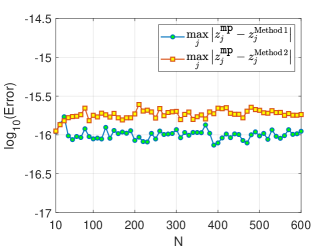
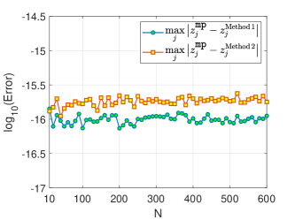
Figure 6.1. Errors between the eigenvalues computed by two algorithms (with double precision) and reference values (with multiple precision) for $\alpha=2$ (left) and $\alpha=4$ (right).

7. Space-time spectral methods

The findings from previous eigenvalue analysis have deep implications in spectral methods in time. In this section, we first present a general framework for the LDPG time discretisation of evolutionary PDEs with a focus on two techniques: (i) matrix diagonalisation and (ii) QZ decomposition (or generalised Schur decomposition) to effectively deal with the resulted matrices. We then apply the space-time spectral methods to some interesting linear and nonlinear wave problems that require high accuracy in both space and time.

7.1. A general framework for the LDPG spectral method in time

We demonstrate the algorithm via the system of linear ODEs:

$$\boldsymbol{u}^{\prime}(t)+\boldsymbol{A}\boldsymbol{u}(t)=\boldsymbol{f}(t),\;\;t\in(-1,1);\quad\boldsymbol{u}(-1)=\boldsymbol{u}_{0},$$ (7.1)

where $\boldsymbol{u},\boldsymbol{f},\boldsymbol{u}_{0}\in{\mathbb{R}}^{N_{x}}$ and $\boldsymbol{A}\in{\mathbb{R}}^{N_{x}\times N_{x}}$ (which might be resulted from spatial discretisations).

Using the LDPG scheme described in Subsection 3.1 to (7.1), we seek the LDPG spectral approximation in terms of the basis (3.3),

$$\boldsymbol{u}(t)\approx\boldsymbol{u}_{*}(t)=\boldsymbol{u}_{0}+\sum_{k=0}^{N_{t}-1}\hat{\boldsymbol{u}}_{k}\phi_{k}(t),$$

and denote the matrix of unknowns by $\widehat{\boldsymbol{U}}=(\hat{\boldsymbol{u}}_{0},\cdots,\hat{\boldsymbol{u}}_{N_{t}-1})^{\top}\in{\mathbb{R}}^{N_{t}\times N_{x}}.$ Then the corresponding linear system reads

$$\widehat{\boldsymbol{U}}+\boldsymbol{M}_{t}\,\widehat{\boldsymbol{U}}\boldsymbol{A}^{\top}=\boldsymbol{F},$$ (7.2)

where $\boldsymbol{M}_{t}\in{\mathbb{R}}^{N_{t}\times N_{t}}$ is the same as in (3.5) and

$$\boldsymbol{F}=\boldsymbol{U}_{0}\boldsymbol{A}^{\top}+(\boldsymbol{\hat{f}}_{0},\cdots,\boldsymbol{\hat{f}}_{N_{t}-1})^{\top}\in{\mathbb{R}}^{N_{t}\times N_{x}},\quad\boldsymbol{U}_{0}=\sqrt{2}\boldsymbol{e}_{1}\boldsymbol{u}_{0}^{\top},\;\;\boldsymbol{\hat{f}}_{j}=(\boldsymbol{f},\phi_{j}^{*}),$$

with the basis functions $\{\phi_{j}^{*}\}$ given in (3.4).

The linear system (7.2) in a moderate scale can be solved directly by rewriting it in the Kronecker product form, but it is costly in particular for multiple spatial dimensions in space, as the time discretisation is globally implicit. In the following, we introduce two techniques to alleviate this burden.

7.1.1. Matrix diagonalisation

Let

$$\boldsymbol{E}=(\boldsymbol{v}_{1},\cdots,\boldsymbol{v}_{N_{t}}),\quad\boldsymbol{\Lambda}={\rm diag}(\lambda_{1},\cdots,\lambda_{N_{t}}),\;\;\;\text{so}\;\;\;\boldsymbol{M}_{t}\,\boldsymbol{E}=\boldsymbol{E}\boldsymbol{\Lambda},$$

where $\{\lambda_{j},\boldsymbol{v}_{j}\}_{j=1}^{N_{t}}$ are eigen-pairs of $\boldsymbol{M}_{t}$ given in Theorem 3.1. Introducing the substitution $\widehat{\boldsymbol{U}}=\boldsymbol{E}\boldsymbol{W},$ we obtain from (7.2) that

$$\boldsymbol{W}-\boldsymbol{\Lambda}\boldsymbol{W}\boldsymbol{A}^{\top}=\boldsymbol{E}^{-1}\boldsymbol{F}=:{\boldsymbol{G}},$$ (7.3)

which can be decoupled and solved in parallel

$$\big{(}\boldsymbol{I}_{\!N_{x}}-\lambda_{j}\boldsymbol{A}\big{)}\boldsymbol{w}_{j}=\boldsymbol{g}_{j},\quad 1\leq j\leq N_{t},$$ (7.4)

where $\boldsymbol{w}_{j},\boldsymbol{g}_{j}$ are the $j$th column of $\boldsymbol{W}^{\top},\boldsymbol{G}^{\top},$ respectively.

Remark 7.1.

Different from a normal matrix, we see from (7.3) that the diagonalisation of a non-normal matrix involves the inverse of the eigenvector matrix $\boldsymbol{E}$. In practice, we can evaluate $\boldsymbol{G}$ by solving the linear system $\boldsymbol{E}{\boldsymbol{G}}=\boldsymbol{F}$ via a suitable iterative solver. It is known that the stability and round-off errors essentially rely on the conditioning of $\boldsymbol{E}.$ Unfortunately, this eigenvector matrix is extremely ill-conditioned with an exponential growth condition number, see Figure 7.2 below. As a result, this technique needs to be implemented in a multi-domain manner with relatively small $N_{t}$ on each sub-domain.

7.1.2. QZ (or generalised Schur) decomposition

Recall that given square matrices $\boldsymbol{A}$ and $\boldsymbol{B}$, the QZ decomposition factorizes both matrices as $\boldsymbol{Q}\boldsymbol{A}\boldsymbol{Z}=\boldsymbol{S}$ and $\boldsymbol{Q}\boldsymbol{B}\boldsymbol{Z}=\boldsymbol{T},$ where $\boldsymbol{Q}$ and $\boldsymbol{Z}$ are unitary (i.e., $\boldsymbol{Q}^{-1}=\boldsymbol{Q}^{\rm H},\boldsymbol{Z}^{-1}=\boldsymbol{Z}^{\rm H},$ where $\boldsymbol{Q}^{\rm H}$ stands for the conjugate transpose or Hermitian transpose of $\boldsymbol{Q}$), and $\boldsymbol{S}$ and $\boldsymbol{T}$ are upper triangular.

We now apply the QZ decomposition to $\boldsymbol{A}=\boldsymbol{I}_{\!N_{t}}$ and $\boldsymbol{B}=\boldsymbol{M}_{t},$ and obtain

$$\boldsymbol{Q}\boldsymbol{Z}=\boldsymbol{S},\quad\boldsymbol{Q}\boldsymbol{M}_{\!t}\boldsymbol{Z}=\boldsymbol{T}.$$ (7.5)

Introducing $\widehat{\boldsymbol{U}}=\boldsymbol{Z}\boldsymbol{W},$ and multiplying both sides of (7.2) by $\boldsymbol{Q},$ we obtain from (7.5) that

$$\boldsymbol{S}\boldsymbol{W}-\boldsymbol{T}\boldsymbol{W}\boldsymbol{A}^{\top}=\boldsymbol{Q}\boldsymbol{F}=:\boldsymbol{G}.$$ (7.6)

As $\boldsymbol{S},\boldsymbol{T}$ are upper triangular matrices, direct backward substitution reduces (7.6) to

$$\boldsymbol{w}_{j}\big{(}S_{jj}\boldsymbol{I}_{\!N_{x}}-T_{jj}\boldsymbol{A}^{\top}\big{)}=\boldsymbol{g}_{j}-\boldsymbol{r}_{j},\quad j=N_{t},N_{t}-1,\cdots,1,$$ (7.7)

where $\boldsymbol{w}_{j},\boldsymbol{g}_{j}$ are the $j$th row of $\boldsymbol{W},\boldsymbol{G}$, and

$$\boldsymbol{r}_{N_{t}}=\boldsymbol{0},\quad\boldsymbol{r}_{j}=\sum_{k=j+1}^{N_{t}}\boldsymbol{w}_{k}\big{(}S_{jk}\boldsymbol{I}_{\!N_{x}}-T_{jk}\boldsymbol{A}^{\top}\big{)},\;\;\;j=N_{t}-1,\cdots,1.$$

Here, $S_{jk},T_{jk}$ with $j\leq k$ are the entries of $\boldsymbol{S},\boldsymbol{T},$ respectively.

Remark 7.2.

The QZ decomposition is stable for large $N_{t}$ and different from (7.3), the step (7.6) does not involve any matrix inversion. Moreover, this technique can be assembled into a multi-domain approach and march sequentially in time. However, as $\{\boldsymbol{r}_{j}\}$ involves $\boldsymbol{w}_{k}$ with $k>j,$ the linear systems (7.7) can only be solved sequentially.

7.2. Space-time spectral methods for linear and nonlinear wave propagations

7.2.1. A linear wave-type equation

As the first example of applications, we consider the linear wave-type equation

$$\begin{dcases}\partial_{xt}^{2}u(x,t)+\sigma u(x,t)=0,\quad x\in\Omega:=(x_{L},x_{R}),\;\;t\in(0,T],\\ u(x,0)=u_{0}(x),\;\;x\in\Omega;\quad u(x_{L},t)=0,\;\;t\in[0,T],\end{dcases}$$ (7.8)

for a given constant $\sigma>0.$ It is of hyperbolic type since under the transformation, we have

$$\partial_{xt}^{2}u(x,t)=\partial_{\xi}^{2}v(\xi,\eta)-\partial_{\eta}^{2}v(\xi,\eta),\quad u(x,t):=v(x+t,x-t).$$

As shown in [29], it is related to the linear Kadomtsev-Petviashvili (KP) model, and the wave propagates along one side if the initial data is compactly supported. More precisely, if $\sigma>0$ and the initial value $u_{0}(x)$ is compactly supported in $(x_{0},\infty),$ then $u(x,t)=0$ for all $x<x_{0}$ and $t\geq 0.$ Thus, we can impose the left-sided boundary condition in (7.8), and then simulate the waves in a finite domain. We transform (7.8) in $\Omega\times(0,T)$ to the reference square $\Lambda:=(-1,1)^{2}$ by simple linear transformations that lead to the same equation but with $\hat{\sigma}={4\sigma}/((x_{R}-x_{L})T)$ in place of $\sigma.$

Applying the LDPG method in Subsection 3.1 for spatial discretisation, we can obtain the system (7.1) of the form

$$\boldsymbol{u}^{\prime}(t)+\hat{\sigma}\boldsymbol{M}_{x}\boldsymbol{u}(t)=\boldsymbol{0},\;\;t\in(-1,1);\quad\boldsymbol{u}(-1)=\boldsymbol{u}_{0},$$ (7.9)

where $\boldsymbol{M}_{x}\in{\mathbb{R}}^{N_{x}\times N_{x}}$ is given in (3.5). Then the general setup detailed in Subsection 7.1 directly carries over to (7.9). We now test the proposed LDPG space-time spectral method and choose

$$u_{0}(x)={\rm sech}^{2}\big{(}\sqrt{3}(x+35)/6\big{)}-{\rm sech}^{2}(5\sqrt{3}/2),\quad x\in\Omega=(-50,50).$$ (7.10)

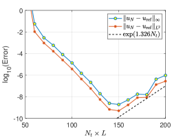
(a) Diagonalisation (multi-domain in $t$)

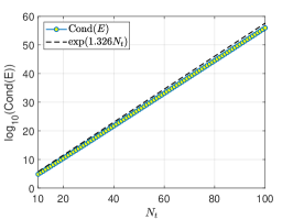
(b) Conditioning of $\boldsymbol{E}$

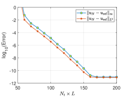
(c) QZ (multi-domain in $t$)

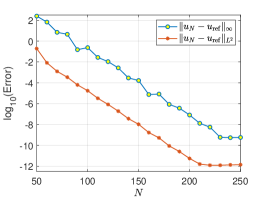
(d) QZ (single domain in $t$)

Figure 7.1. Convergence of space-time spectral methods and conditioning of the eigenvector matrix (in (b)).​ (a) Diagonalisation technique; (c) QZ decomposition with a multi-domain implementation: $L=10$ subintervals of $t\in[0,40]$ with various $N_{t}\in[5,20]$ and $N_{x}=400.$ (d) Single domain space-time spectral method with various $N=N_{t}=N_{x}.$

We first check the accuracy of the solvers with the reference solution (denoted by $u_{\rm ref}$) obtained from the scheme with sufficiently large $N_{t}=N_{x}=400$ and up to $T=40$ in time. As the diagonalisation technique works for small $N_{t}$, we partition the time interval $[0,T]$ equally into $L$ sub-intervals (but with the same $N_{t}$ on each subinterval). Now, we vary $N_{t}$ from $5$ to $20$ and fix $L=10$ and $N_{x}=400.$ We plot in Figure 7.1 (a) (resp. Figure 7.1 (c)) the discrete $L^{\infty}$- and $L^{2}$-errors for the spectral solver with diagonalisation (resp. QZ decomposition) in the semi-log scale. We observe from Figure 7.1 (a) that the errors of the diagonalisation technique for $N_{t}$ up to $15$ decay exponentially, but grow exponentially for $16\leq N_{t}\leq 20.$ Surprisingly, the growth rate agrees well with that of the condition number of the eigenvector matrix $\boldsymbol{E},$ illustrated in Figure 7.1 (b). However, the QZ decomposition in the same setting is stable and accurate for all samples of $N_{t},$ as shown in Figure 7.1 (c). We also depict in Figure 7.1 (d) the errors of the QZ decomposition with a single domain in $t$ and $N=N_{t}=N_{x}$ for various $N,$ from which we observe an exponential convergence rate.

We now use the space-time spectral solver with QZ decomposition in time to simulate the wave propagations. In the computation, we take $N_{t}=N_{x}=400.$ Observe from Figure 7.2 (a) that the initial input (7.10) immediately disperses and spreads in both space and time that leads to oscillations and the waves decay in space at certain algebraic rate (refer to [29] for detailed analysis).

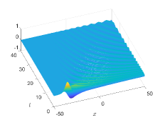
(a) $u_{N}(x,t)$ with $\sigma=1$

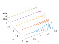
(b) $u_{N}(x,40)$ with different $\sigma$

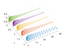
(c) $u_{N}(50,t)$ with different $\sigma$

Figure 7.2. Numerical solutions $u_{N}(x,t)$ obtained by (7.8) given the initial profile (7.10) with $N_{x}=N_{t}=400$ and different values of the parameter $\sigma.$ (a) Numerical solution with $\sigma=1$; (b)-(c) Profiles of the numerical solution at fixed $t$ or $x$ but with different $\sigma.$

It is important to point out that the coefficient matrices of linear systems (7.4) and (7.7) in space are well-conditioned. In Table 7.1, we tabulate the condition numbers and eigenvalues with the minimum and maximum moduli of the matrix $\boldsymbol{A}:=\boldsymbol{I}_{\!N_{x}}+\boldsymbol{M}_{x}.$

Table 7.1. Conditioning and eigenvalues of $\boldsymbol{A}=\boldsymbol{I}_{\!N_{x}}+\boldsymbol{M}_{x}.$

$N_{x}$	$20$	$30$	$40$	$50$	$100$	$200$
${\rm Cond}(\boldsymbol{A})$	1.8730	1.8730	1.8730	1.8730	1.8730	1.8730
$\min_{j}|\lambda_{j}^{\boldsymbol{A}}|$	1.0143	1.0071	1.0043	1.0029	1.0009	1.0003
$\max_{j}|\lambda_{j}^{\boldsymbol{A}}|$	1.0708	1.0513	1.0539	1.0533	1.0513	1.0514

7.2.2. A nonlinear KdV-type equation

As a second example, we apply the space-time LDPG method to the KdV-type equation:

$$\begin{dcases}\partial_{t}U+\alpha U\partial_{x}U+\epsilon^{2}\partial_{x}^{3}U+\sigma\partial_{x}^{-1}U=0,\quad&x\in\Omega:=(x_{L},x_{R}),\;\;t\in(0,T]\\ U(x_{L},t)=U(x_{R},t)=\partial_{x}U(x_{R},t)=0,\quad&t\in[0,T],\\ U(x,0)=U_{0}(x),\quad&x\in\bar{\Omega},\end{dcases}$$ (7.11)

where $\alpha\geq 0,\epsilon>0$ and $\sigma\not=0$ are constants, and

$$\partial_{x}^{-1}U(x,t)=\frac{1}{2}\Big{(}\int_{x_{L}}^{x}U(y,t){\rm d}y-\int_{x}^{x_{R}}U(y,t){\rm d}y\Big{)}.$$

It also relates to the reduced KP equations [29]. Like before, we covert (7.11) to the reference square $(-1,1)^{2},$ and then follow Shen [18] to formulate the LDPG in space involving the pair of dual spaces

$$\begin{split}{\mathbb{V}}_{\!N_{x}}&:=\big{\{}\phi\in\mathbb{P}_{N_{x}+2}:\phi(-1)=\phi(1)=\phi^{\prime}(1)=0\big{\}},\\ {\mathbb{V}}_{\!N_{x}}^{*}&:=\big{\{}\psi\in\mathbb{P}_{N_{x}+2}:\psi(-1)=\psi(1)=\psi^{\prime}(-1)=0\big{\}}.\end{split}$$

We omit the details on the expressions of the basis functions and formulation of the matrix form. In the numerical tests, we use the Newton’s iteration to solve the resulting nonlinear system when $\alpha\not=0.$ Consider (7.11) with the initial condition given by

$$U_{0}(x)={\rm sech}^{2}\big{(}\sqrt{3}(x+5)/6\big{)},\quad x\in\Omega=(-50,50),$$ (7.12)

taken from the soliton solution of the KdV equation (i.e., (7.11) with $\alpha=\epsilon=1$ and $\sigma=0$):

$$U(x,t)={\rm sech}^{2}\big{(}\sqrt{3}(x-t/3+5)/6\big{)}.$$

We first show the accuracy by solving the KdV equation in the domain $\Omega\times(0,20).$ In Figure 7.3, we plot the numerical solution and the discrete $L^{\infty}$- and $L^{2}$-errors with $N_{t}=80$ and various $N_{x}=50:10:200,$ which shows a spectral accuracy.

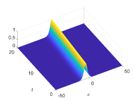
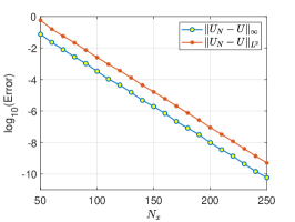
Figure 7.3. Left: numerical solution $u_{N}(x,t)$ (with $N_{x}=250,N_{t}=80$) of the KdV equation (i.e., (7.11) with $\alpha=\epsilon=1$ and $\sigma=0$) for given initial input in (7.12). Right: Errors against $N_{x}=50:10:250$ and fixed $N_{t}=80$ in semi-log scale.

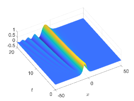
(a) Linear KdV

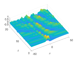
(b) KdV with a nonlocal term

Figure 7.4. Numerical solutions with $N_{x}=250,N_{t}=80$ and the initial input $U_{0}(x)$ given in (7.12). (a) Linear KdV equation (i.e., (7.11) with $\epsilon=1$ and $\alpha=\sigma=0$). (b) KdV-type equation with a nonlocal term (i.e., (7.11) with $\alpha=0,\epsilon=1$ and $\sigma=0.1$).

Using the accurate space-time spectral solver, we simulate the wave propagations for the linear KdV equation and (7.11) with a nonlocal term under the same setting. We plot the numerical solutions in Figure 7.4 and find that for the linear KdV equation, the initial wave spreads out only on the left side of the soliton wave of the nonlinear KdV equation (see Figure 7.3 (left)) and induces some wiggles. However, when there is a nonlocal integral term, the initial wave immediately propagates chaotically without a clear pattern.

8. Concluding remarks

In this paper, we showed that the eigen-pairs of spectral discretisation matrices resulted from the LDPG methods for prototype $m$th-order IVPs are associated with the GBPs. More precisely, we were able to exactly characterize the eigenvalues and eigenvectors for $m=1,2$, and approximately characterize the eigenvalues and eigenvectors for $m=3$. We also showed that by reformulating of the $m$th-order ($m>3$) IVP as a first-order system, the eigenvalues and eigenvectors of the matrix can be exactly characterized by zeros of the GBP: $B_{N}^{(3)}(z).$

As a by-product, we identified the eigen-pairs of the spectral-collocation differentiation matrix at the Legendre points by reformulating the collocation scheme into a Petrov-Galerkin formulation, and provided answers to some open questions in literature related to this special collocation method.

The findings in this paper have direct implication on developing LDPG spectral methods in time. As an application, we proposed a general framework to construct space-time spectral methods for a class of time dependent PDEs, and presented two alternatives, matrix diagonalisation which is fully parallel but is limited to a small number of unknowns in time due to the ill conditioning and QZ decomposition which is stable at large size but involves sequential computations, for their efficient implementation.

References

- [1] T.Z. Boulmezaoud and J.M. Urquiza. On the eigenvalues of the spectral second order differentiation operator and application to the boundary observability of the wave equation. J. Sci. Comput., 31(3):307–345, 2007.
- [2] C. Canuto, M.Y. Hussaini, A. Quarteroni, and T.A. Zang. Spectral Methods in Fluid Mechanics. Springer-Verlag, New York, 1988.
- [3] C. Canuto, M.Y. Hussaini, A. Quarteroni, and T.A. Zang. Spectral Methods: Fundamentals in Single Domains. Springer, Berlin, 2006.
- [4] G. Csordas, M. Charalambides, and F. Waleffe. A new property of a class of Jacobi polynomials. Proc. Amer. Math. Soc., 133(12):3551–3560, 2005.
- [5] M.G. de Bruin, E.B. Saff, and R.S. Varga. On the zeros of generalized Bessel polynomials. I and II. Indag. Math., 43(1):1–25, 1981.
- [6] M. Dubiner. Asymptotic analysis of spectral methods. J. Sci. Comput., 2(1):3–31, 1987.
- [7] D. Gottlieb and L. Lustman. The spectrum of the Chebyshev collocation operator for the heat equation. SIAM J. Numer. Anal., 20:909–921, 1983.
- [8] D. Gottlieb and S.A. Orszag. Numerical Analysis of Spectral Methods: Theory and Applications. SIAM-CBMS, Philadelphia, 1977.
- [9] E. Grosswald. Bessel Polynomials. Springer Berlin Heidelberg, 1978.
- [10] J. Shen and L.-L. Wang. Fourierization of the Legendre-Galerkin method and a new space-time spectral method. Appl. Numer. Math., 57:710–720, 2007.
- [11] H. L. Krall and O. Frink. A new class of orthogonal polynomials: The Bessel polynomials. Trans. Am. Math. Soc., 65(1):100–115, 1949.
- [12] J. Liu, X. Wang, S. Wu, and T. Zhou. A well-conditioned direct PinT algorithm for first-and second-order evolutionary equations. Adv. Comput. Math., 48:16, 2022.
- [13] S. H. Lui. Legendre spectral collocation in space and time for PDEs. Numer. Math., 136(1):75–99, 2016.
- [14] Y. Maday and E. M. Rønquist. Parallelization in time through tensor-product space-time solvers. C. R. Acad. Sci. Paris, Ser. I, 346(1-2):113–118, 2008.
- [15] L. Pasquini. On the computation of the zeros of the Bessel polynomials. In Approximation and Computation: A Festschrift in Honor of Walter Gautschi, pages 511–534. Birkhäuser Boston, 1994.
- [16] L. Pasquini. Accurate computation of the zeros of the generalized Bessel polynomials. Numer. Math., 86(3):507–538, 2000.
- [17] J. Segura. Computing the complex zeros of special functions. Numer. Math., 124(4):723–752, 2013.
- [18] J. Shen. A new dual-Petrov-Galerkin method for third and higher odd-order differential equations: Application to the KDV equation. SIAM J. Numer. Anal, 41(5):1595–1619, 2003.
- [19] J. Shen and C.-T. Sheng. An efficient space-time method for time fractional diffusion equation. J. Sci. Comput., 81(2):1088–1110, 2019.
- [20] J. Shen, T. Tang, and L.-L. Wang. Spectral Methods: Algorithms, Analysis and Applications. Springer-Verlag, New York, 2011.
- [21] J. Shen and L.-L. Wang. Legendre and Chebyshev dual-Petrov-Galerkin methods for hyperbolic equations. Comput. Methods Appl. Mech. Eng., 196(37-40):3785–3797, 2007.
- [22] H. Tal-Ezer. A pseudospectral Legendre method for hyperbolic equations with an improved stability condition. J. Comput. Phys., 67(1):145–172, 1986.
- [23] H. Tal-Ezer. Spectral methods in time for hyperbolic equations. SIAM J. Numer. Anal., 23(1):11–26, 1986.
- [24] H. Tal-Ezer. Spectral methods in time for parabolic problems. SIAM J. Numer. Anal., 26(1):1–11, 1989.
- [25] J.-G. Tang and H.-P. Ma. Single and multi-interval Legendre -methods in time for parabolic equations. Adv. Comput. Math., 17(4):349–367, 2002.
- [26] J.-G. Tang and H.-P. Ma. A Legendre spectral method in time for first-order hyperbolic equations. Appl. Numer. Math., 57(1):1–11, 2007.
- [27] L.N. Trefethen and M.R. Trummer. An instability phenomenon in spectral methods. SIAM J. Numer. Anal., 24(5):1008–1023, 1987.
- [28] J. Wang and F. Waleffe. The asymptotic eigenvalues of first-order spectral differentiation matrices. J. Appl. Math. Phys., 02(05):176–188, 2014.
- [29] X. P. Wang, D. S. Kong, and L.-L. Wang. Numerical study of the linear KdV and Kadomtsev-Petviashvili equations in oscillatory regimes. In preparation, 2022.
- [30] J.A.C. Weideman and L.N. Trefethen. The eigenvalues of second-order spectral differentiation matrices. SIAM J. Numer. Anal., 25(6):1279–1298, 1988.
- [31] Z. Zhang. How many numerical eigenvalues can we trust? J. Sci. Comput., 65(2):455–466, 2014.