The Information-State Based Approach to Linear System Identification

Abstract

This paper considers the problem of system identification for linear systems. We propose a new system realization approach that uses an “information-state” as the state vector, where the “information-state” is composed of a finite number of past inputs and outputs. The system identification algorithm uses input-output data to fit an autoregressive moving average model (ARMA) to represent the current output in terms of finite past inputs and outputs. This information-state-based approach allows us to directly realize a state-space model using the estimated ARMA or time-varying ARMA parameters for linear time invariant (LTI) or linear time varying (LTV) systems, respectively. The paper develops the theoretical foundation for using ARMA parameters-based system representation using only the concept of linear observability, details the reasoning for exact output modeling using only the finite history, and shows that there is no need to separate the free and the forced response for identification. The proposed approach is tested on various different systems, and the performance is compared with state-of-the-art system identification techniques.

I Introduction

In this paper, we consider the system identification of linear systems. The motivation for the work arose while we were trying to accomplish the data-based optimal control of nonlinear systems where we had introduced a linear time varying (LTV) system identification technique based on an auto regressive moving average (ARMA) model of the input output map of an LTV system [1]. Nonlinear dynamical systems can be approximated either as a linear time-invariant (LTI) system around an equilibrium or a linear time-varying (LTV) system around a trajectory. System identification has to be done to design control laws for such systems [2, 3]. System identification techniques have also been used for parameter identification and for generating reduced-order models [4, 5]. The technique discussed in this paper, building upon the preliminary idea introduced in [1], uses a novel system realization that is based on the “information-state” as the state vector. An ARMA model which can represent the current output in terms of inputs and outputs from $q$ steps in the past, is found by solving a linear regression problem relating the input and output data. Defining the state vector to be the past $q$ inputs and outputs, as the information-state, lets us realize a state-space model directly using the estimated time-varying ARMA parameters.

The pioneering work in system identification for LTI systems is the Ho-Kalman realization theory [6] of which the Eigensystem Realization Algorithm (ERA) algorithm is one of the most popular  [4]. Another system identification method, namely, q-Markov covariance equivalent realization, generates a stable LTI system model which matches the first “q” Markov parameters of the underlying system and also matches the equivalent steady-state covariance response/ parameters of the identified system [7, 8]. These algorithms assume stable systems so that the response can be modeled using only a small finite set of parameters relating the past inputs to the current output (moving-average (MA) model). For lightly damped and marginally stable systems, the length of history to be considered and the parameters to be estimated becomes very long, leading to numerical issues when solving for the parameters. To overcome this issue, the observer Kalman identification algorithm (OKID) [9] uses an ARMA model, rather than an MA model, consisting of past outputs and controls to model the current output. The time-varying counterparts of the ERA and OKID - TV-ERA and TV-OKID - were developed in [10] and [11], respectively. The identification of time varying linear systems (TV-ERA and TV-OKID) also builds on the earlier work on time-varying discrete time system identification [5, 12]. The OKID and TV-OKID explain the usage of an ARMA model to be equivalent to an observer in the loop system, and postulate that the identified observer is a deadbeat observer similar to the work in [13].

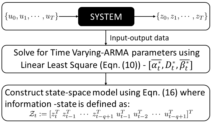
Figure 1: Steps involved in system identification using Information-state approach.

All the algorithms mentioned above start by estimating the Markov parameters of the system from input-output data: the ERA type techniques directly from the MA model and the OKID methods from recursively solving a set of linear equations involving the ARMA/ observer Markov parameters. A Hankel matrix is built using the estimated Markov parameters, and a singular value decomposition (SVD) of the Hankel matrix is used to find the system matrices. Most of them either require the experiments to be performed from zero-initial conditions or wait sufficiently long enough for the initial condition response to die out. The time-varying systems also need an additional step of coordinate transformation, as the realized matrices at different time steps are in different coordinate frames [10]. These Hankel SVD-based approaches for LTV systems also require separate experiments - forced response with zero-initial conditions and a free-response with random initial conditions, where the free response experiments are required to identify the system in the first and last few steps.

Contributions: The main contributions of this work are: (i) the usage of “information-state” as the state-vector which helps to arrive at the state-space realization directly from the ARMA parameters for both time-invariant and time-varying cases, without the need for the formation of a Hankel matrix and its SVD. The time-varying case is especially interesting, as the system realization method is exactly the same as the time-invariant case, and doesn’t require any coordinate transformations as required in the previous literature [10, 11]; (ii) a new explanation of why the ARMA model can predict the output from a finite history of inputs and outputs for any linear system based on linear observability, without recourse to a hypothesized deadbeat observer as in [9, 11]; and (iii) the approach avoids the need to perform separate experiments for the forced response from zero initial conditions and the free-response from random initial conditions, i.e., there is no need to separate the forced and the free response for identification.
The rest of the paper is structured as follows: Section II introduces the problem; Section III develops the theory for the information-state approach and provides new insight for the ARMA parameters; Owing to the similarities of our work with the OKID/ TV-OKID approaches, Section IV is dedicated to show the relationship and differences between the approaches, in particular, the non-necessity of using an observer in the loop to explain the ARMA model; In section V, we show examples where we apply the approach to a true LTV system and also show its capability of identifying nonlinear systems along a finite trajectory; while Section VI draws conclusions about our work.

II Problem Formulation

Consider a linear time-varying system given as:

$$x_{t+1} =A_{t}x_{t}+B_{t}u_{t},$$

$$z_{t} =C_{t}x_{t}+D_{t}u_{t},$$ (1)

where $x_{t}\in\mathbb{R}^{n}$ is the state, $u_{t}\in\mathbb{R}^{r}$ is the input, and $z_{t}\in\mathbb{R}^{m}$ is the output of the system, defined for $\forall\ t\geq 0$. Given the input-output data from such a system with unknown initial conditions, the problem of system identification deals with finding matrices $\mathcal{A}_{t}$, $\mathcal{B}_{t}$, $\mathcal{C}_{t}$, $D_{t}$ such that the new system:

$$\tilde{x}_{t+1} =\mathcal{A}_{t}\tilde{x}_{t}+\mathcal{B}_{t}u_{t},$$

$$z_{t} =\mathcal{C}_{t}\tilde{x}_{t}+D_{t}u_{t},$$ (2)

has the same input-output and transient response as the original system (given in Eq. (1)). The dimension of state $\tilde{x}_{t}$ for the identified system need not be necessarily the same as the dimension of state $x_{t}$, and thus the dimension of the system matrices $\mathcal{A}_{t},\mathcal{B}_{t}$ and $\mathcal{C}_{t}$ can also be different from the underlying system matrices.

III Information-State based System Identification: Theory

In this section, we shall present the theoretical foundation for the information-state based approach for the identification of linear time-varying systems described in Eq. (1).

Definition 1

Information-state. The information-state of the system in Eq. (1) of order $``q"$ (at time $t$) is defined as $\mathcal{Z}_{t}={[z_{t-1},z_{t-2},\cdots,z_{t-q},u_{t-1},u_{t-2},\cdots,u_{t-q}]}^{\mathsf{T}}$.

First, we show the following basic result that is key to the entire development.

Assumption 1

Observability. We assume that the system in Eq. (1) is uniformly observable for all time $t$, i.e., the observability matrix:

$$O^{q}_{t-1}=\begin{bmatrix}C_{t-1}A_{t-2}\cdots A_{t-q}\\ C_{t-2}A_{t-3}\cdots A_{t-q}\\ \vdots\\ C_{t-q}\\ \end{bmatrix},$$ (3)

is rank $n$ for any $q$ such that $mq\geq n$.

Proposition 1

Given the linear system in Eq. (1), under Assumption 1, there exists an ARMA model such that:

$$z_{t} =\alpha^{(q)}_{t-1}z_{t-1}+\alpha^{(q)}_{t-2}z_{t-2}+\cdots+\alpha^{(q)}_{t-q}z_{t-q}$$

$$~{}~{}~{}~{}+\beta^{(q)}_{t-1}u_{t-1}+\beta^{(q)}_{t-2}u_{t-2}+\cdots+\beta^{(q)}_{t-q}u_{t-q},$$ (4)

for any $q\leq t$, and for time $t$ such that $mt\geq n$.

$$\underbrace{\begin{bmatrix}z_{t-1}\\ z_{t-2}\\ \vdots\\ z_{t-q}\end{bmatrix}}_{Z^{q}_{t-1}}=\underbrace{\begin{bmatrix}C_{t-1}A_{t-2}\cdots A_{t-q}\\ C_{t-2}A_{t-3}\cdots A_{t-q}\\ \vdots\\ C_{t-q}\end{bmatrix}}_{O_{t-1}^{q}}x_{t-q}+\underbrace{\begin{bmatrix}D_{t-1}&C_{t-1}B_{t-2}&\cdots&\cdots&C_{t-1}A_{t-2}...B_{t-q}\\ 0&D_{t-2}&C_{t-2}B_{t-3}&\cdots&C_{t-2}A_{t-3}...B_{t-q}\\ \vdots&\vdots&\ddots&\cdots&\vdots\\ 0&0&0&\cdots&D_{t-q}\end{bmatrix}}_{G_{t-1}^{q}}\underbrace{\begin{bmatrix}u_{t-1}\\ u_{t-2}\\ \vdots\\ u_{t-q}\end{bmatrix}}_{U^{q}_{t-1}}.$$ (5)

Proof:

Note that the outputs of the system can be written as shown in Eq. (5) (next page). From Eq. (5), it follows that (under Assumption 1 and for $mt\geq n$):

$$x_{t-q}=(O_{t-1}^{q})^{\dagger}(Z^{q}_{t-1}-G_{t-1}^{q}U^{q}_{t-1}),$$

since $O_{t-1}^{q}$ has rank $n$ owing to Assumption 1. The symbol $\dagger$ represents the Moore-Penrose inverse. Then,

$$z_{t} =C_{t}A_{t-1}...A_{t-q}x_{t-q}$$

$$+[C_{t}B_{t-1},\cdots,C_{t}A_{t-1}\cdots B_{t-q}]U^{q}_{t-1}+D_{t}u_{t},$$ (6)

$$z_{t} =C_{t}A_{t-1}...A_{t-q}(O_{t-1}^{q})^{\dagger}Z^{q}_{t-1}+([C_{t}B_{t-1},\cdots,$$

$$C_{t} A_{t-1}\cdots B_{t-q}]-C_{t}A_{t-1}...A_{t-q}(O_{t-1}^{q})^{\dagger}G_{t-1}^{q})U^{q}_{t-1}+D_{t}u_{t}.$$ (7)

From Eq. (7), it is clear that the ARMA model is given by:

$$z_{t} =\alpha_{t-1}z_{t-1}+\cdots+\alpha_{t-q}z_{t-q}$$

$$+D_{t}u_{t}+\beta_{t-1}u_{t-1}+\cdots+\beta_{t-q}u_{t-q},$$ (8)

where,

$$[\alpha_{t-1}\cdots\alpha_{t-q}] =C_{t}A_{t-1}...A_{t-q}(O_{t-1}^{q})^{\dagger},$$

$$[\beta_{t-1}\cdots\beta_{t-q}] =([C_{t}B_{t-1},\cdots,C_{t}A_{t-1}\cdots B_{t-q}]$$

$$-C_{t}A_{t-1}...A_{t-q}(O_{t-1}^{q})^{\dagger}G_{t-1}^{q}).$$ (9)

This concludes the proof. ∎

Next, we show that the above “TV-ARMA” model is capable of predicting the output $z_{t}$ for any time $t$ s.t. $mt\geq n$.

Corollary 1

For any time $t$, s.t. $mt\geq n$, the TV-ARMA model (Eq. (8)) can perfectly predict the output $``z_{t}"$ of the linear system (Eq. (1)).

Proof:

By construction, TV-ARMA (Eq. (8)) is capable of predicting $z_{t}$. Noting that $O_{t-1}^{q}$ becomes rank “$n$” for time $t$, for $mt\geq n$, the result follows. ∎

Next, we show how to find the TV-ARMA model of order $q$ by setting up the problem. We may write

$$\underbrace{\begin{bmatrix}z_{t}^{(1)}~{}\cdots~{}z_{t}^{(N)}\end{bmatrix}}_{Z_{t}^{(1:N)}}=\underbrace{\begin{bmatrix}\alpha^{q}_{t,t-1}~{}\cdots~{}\alpha^{q}_{t,t-q}\end{bmatrix}}_{\bar{\alpha}_{t}}\begin{bmatrix}z_{t-1}^{(1)}&\cdots&z_{t-1}^{(N)}\\ z_{t-2}^{(1)}&\cdots&z_{t-2}^{(N)}\\ \vdots&\ddots&\vdots\\ z_{t-q}^{(1)}&\cdots&z_{t-q}^{(N)}\\ \end{bmatrix}$$

$$~{}~{}~{}~{}~{}~{}+\begin{bmatrix}D_{t}~{}\underbrace{\beta^{q}_{t,t-1}~{}\cdots~{}\beta^{q}_{t,t-q}}_{\bar{\beta}_{t}}\end{bmatrix}\begin{bmatrix}u^{(1)}_{t}&\cdots&u^{(N)}_{t}\\ u^{(1)}_{t-1}&\cdots&u^{(N)}_{t-1}\\ \vdots&\ddots&\vdots\\ u^{(1)}_{t-q}&\cdots&u^{(N)}_{t-q}\\ \end{bmatrix},$$ (10)

where ${z^{(i)}_{t},u^{(i)}_{t}}$ represent the observation and inputs for the $``i^{\text{th}}"$ rollout/experiment.
The order of the state-space model can then be found using the following approach. Let the concatenated data matrix be represented as :

$$\mathcal{X}^{q}_{t}=\begin{bmatrix}z_{t-1}^{(1)}&\cdots&z_{t-1}^{(N)}\\ \vdots&\ddots&\vdots\\ z_{t-q}^{(1)}&\cdots&z_{t-q}^{(N)}\\ u^{(1)}_{t}&\cdots&u^{(N)}_{t}\\ \vdots&\ddots&\vdots\\ u^{(1)}_{t-q}&\cdots&u^{(N)}_{t-q}\end{bmatrix}\in\mathbb{R}^{mq+(q+1)r\times N}.$$ (11)

The data matrix $\mathcal{X}^{q}_{t}$ is a full row rank matrix for $mq<n$, with $n$ being the order of the underlying system. Therefore, the minimum order of the ARMA parameters $q$ is obtained by increasing the order $q$ till the data matrix $\mathcal{X}^{q}_{t}$ becomes row rank deficient. In particular, we can do an SVD of $\mathcal{X}^{q}_{t}$ for some suitably large $q$. The rank of the $\mathcal{X}^{q}_{t}$ is going to be $``n+(q+1)r"$, and thus, the minimal order ARMA model can be found by setting $q^{*}$ s.t. $mq^{*}\geq n$. In particular, for single-output system $(m=1)$, the minimal order $q^{*}=n$. However, in general owing to the fact that $m$ and $n$ need not be integer multiples, i.e., $n\neq mq$ for some integer $q$, the order $q$ of the ARMA model is going to be larger than the state order $n$. The above development may now be summarized as follows.

Proposition 2

Given a data matrix $\mathcal{X}^{q}_{t}$ of order $q$ as in Eq. (11), with $mq>n$, the minimal order ARMA model for system (Eq. (1)) is given by choosing $q^{*}$ s.t. $mq^{*}\geq n$, where $(n+(q+1)r)$ is the rank of $\mathcal{X}^{q}_{t}$.

III-A Solving for the ARMA parameters:

Consider the linear problem:

$$Z^{(1:N)}_{t}=\begin{bmatrix}\bar{\alpha}_{t}&D_{t}&\bar{\beta}_{t}\end{bmatrix}\mathcal{X}^{q}_{t}.$$ (12)

where $Z^{(1:N)}_{t}\in\mathbb{R}^{m\times N}$ indicate the outputs from $N$ rollouts, and $\mathcal{X}^{q}_{t}\in\mathbb{R}^{mq+(q+1)r\times N}$ is the data matrix containing the past outputs and inputs as shown in Eq. (11). The ARMA parameters can be solved by minimizing the least-squares error.
For $q$ s.t. $mq\geq n$, Eq. (12) does not have a unique solution, owing to the row rank-deficiency of $\mathcal{X}^{q}_{t}$. The least-squares solution is the Moore-Penrose inverse of Eq. (12), assuming $N>2q$. Let $\mathcal{X}^{q}_{t}=U\Sigma{V}^{\mathsf{T}}$ where $\Sigma=\begin{bmatrix}\Sigma_{n+(q+1)r}&\\ &\mathbf{0}\\ \end{bmatrix}$, $\Sigma_{n+(q+1)r}=\begin{bmatrix}\sigma_{1}&&0\\ &\ddots&\\ 0&&\sigma_{n+(q+1)r}\end{bmatrix}$, and $V=[V_{1}\ V_{2}]$, $U=[U_{1}\ U_{2}]$, where $(U_{1},\ V_{1})$ are the singular vectors corresponding to the non-zero singular values $\Sigma_{n+(q+1)r}$ and $(U_{2},\ V_{2})$ are the singular vectors corresponding to the zero-singular values, i.e., the singular vectors spanning the nullspace of $\mathcal{X}^{q}_{t}$. The least-squares (LS) solution is:

$$\begin{bmatrix}\bar{\alpha}^{*}_{t}&D^{*}_{t}&\bar{\beta}^{*}_{t}\end{bmatrix}=\sum_{i=1}^{n+(q+1)r}\sigma^{-1}_{i}(Z^{(1:N)}_{t}\mathrm{v}_{i}){\mathrm{u}_{i}}^{\mathsf{T}},$$ (13)

where $\mathrm{u}_{i}$ and $\mathrm{v}_{i}$ are the singular vectors corresponding to $\sigma_{i}$.
A natural question that arises is: What is the relationship between the ARMA model of Eq. (9) and the least-squares problem given by Eq. (12)? First, we show that the ARMA solution (Eq. (9)) satisfies the LS-problem Eq. (12).

Proposition 3

The ARMA solution given by Eq. (9) is a solution of the LS-equation (12).

Proof:

By construction, $z_{t}=\alpha^{\#}_{t,t-1}z_{t-1}+\cdots+D_{t}u_{t}+\beta^{\#}_{t,t-1}u_{t-1}+\cdots+\beta^{\#}_{t,t-q}u_{t-q},$ where $(\alpha^{\#}_{t,t-k},\beta^{\#}_{t,t-k})$ are the solution (9), and it holds for all ${z^{(i)}_{t}}$ ∎

Thus, given the system (1), after time $t$, s.t. $mt\geq n$, the output $z_{t}$ can be predicted by both the LS-solution (13) as well as the ARMA-solution (9). This is summarized in the following corollary.

Corollary 2

Let the solution of Eq. (9) be denoted by $(\bar{\alpha}^{\#}_{t},\bar{\beta}^{\#}_{t})$. Then for any time $t$ s.t. $mt\geq n$,

$$z_{t} =\alpha^{\#}_{t,t-1}z_{t-1}+\cdots+\alpha^{\#}_{t,t-q}z_{t-q}$$

$$+D_{t}u_{t}+\beta^{\#}_{t,t-1}u_{t-1}+\cdots+\beta^{\#}_{t,t-q}u_{t-q}$$ (14)

$$=\alpha^{*}_{t,t-1}z_{t-1}+\cdots+\alpha^{*}_{t,t-q}z_{t-q}$$

$$+D_{t}u_{t}+\beta^{*}_{t,t-1}u_{t-1}+\cdots+\beta^{*}_{t,t-q}u_{t-q}.$$ (15)

An immediate consequence of the above result is that the LS-ARMA model (13) also predicts the response of the linear system (1).

We note here that the LS-solution (13) and the “fundamental solution” (9) need not be the same, nonetheless, both can predict the initial + forced response of the linear system (1) after time $t$ s.t. $mt\geq n$, under the observability assumption 1.
The information-state based state-space model can then be written as in Eq. (16)(next page).

$$\underbrace{\begin{bmatrix}z_{t}\\ z_{t-1}\\ z_{t-2}\\ \vdots\\ z_{t-q+1}\\ \hline\cr u_{t-1}\\ u_{t-2}\\ u_{t-3}\\ \vdots\\ u_{t-q+1}\end{bmatrix}}_{\mathcal{Z}_{t}} =\underbrace{\setcounter{MaxMatrixCols}{11}\begin{bmatrix}\alpha_{t-1}&\alpha_{t-2}&\cdots&\alpha_{t-q+1}&\alpha_{t-q}&\vline&\beta_{t-2}&\beta_{t-3}&\cdots&\beta_{t-q+1}&\beta_{t-q}\\ I_{m\times m}&0&\cdots&0&0&\vline&0&0&\cdots&0&0\\ 0&I&\cdots&0&0&\vline&0&0&\cdots&0&0\\ \vdots&&\ddots&&\vdots&\vline&\vdots&&\ddots&\vdots&0\\ 0&0&\cdots&I&0&\vline&0&0&\cdots&0&0\\ \hline\cr 0&0&\cdots&0&0&\vline&0&0&\cdots&0&0\\ 0&0&\cdots&0&0&\vline&I_{r\times r}&0&\cdots&0&0\\ 0&0&\cdots&0&0&\vline&0&I&\cdots&0&0\\ \vdots&&\ddots&&\vdots&\vline&\vdots&&\ddots&&\vdots\\ 0&0&\cdots&0&0&\vline&0&0&\cdots&I&0\end{bmatrix}}_{\mathcal{A}_{t-1}}\underbrace{\begin{bmatrix}z_{t-1}\\ z_{t-2}\\ \vdots\\ z_{t-q+1}\\ z_{t-q}\\ \hline\cr u_{t-2}\\ u_{t-3}\\ \vdots\\ u_{t-q+1}\\ u_{t-q}\end{bmatrix}}_{\mathcal{Z}_{t-1}}+\underbrace{\begin{bmatrix}\beta_{t-1}\\ 0\\ \vdots\\ 0\\ 0\\ \hline\cr I\\ 0\\ \vdots\\ 0\\ 0\end{bmatrix}}_{\mathcal{B}_{t-1}}u_{t-1}$$ (16)

$$z_{t} =\underbrace{\begin{bmatrix}I_{m\times m}&0&\cdots&0\end{bmatrix}}_{\mathcal{C}_{t}}\mathcal{Z}_{t}+D_{t}u_{t}$$ (17)

It can now be seen that the information-state $\mathcal{Z}_{t}$ is indeed a state of the system (1). In particular, the following result holds:

Proposition 4

Under assumption 1, and for any time $t$, s.t. $mt\geq n$, the output $z^{\prime}_{t}$ of the information-state model in Eq. (16) is equal to the output of the linear state-space model (1), given the same inputs, and regardless of the “unknown” initial condition $x_{0}$.

Proof:

By corollary 2, we know that the output of the linear system (1) after time $t$ s.t. $mt\geq n$ may be written as: $z_{t}=\alpha^{*}_{t,t-1}z_{t-1}+\cdots+\alpha^{*}_{t,t-q}z_{t-q}+D_{t}u_{t}+\beta^{*}_{t,t-1}u_{t-1}+\cdots+\beta^{*}_{t,t-q}u_{t-q}.$ Further $\mathcal{Z}_{t}$ is a state of the system owing to its definition, and thus, noting the definition of the output $z^{\prime}_{t}$ of the information-state system (17), the result immediately follows. ∎

Linear Time Invariant (LTI) Case:

A further simplification of the information-state model is possible if the linear system (1) is LTI (we ignore the $D$ term for sake of simplicity). Since the system is LTI, Eq. (8) becomes $z_{t}=\alpha_{1}z_{t-1}+\alpha_{2}z_{t-2}+\cdots+\alpha_{q}z_{t-q}+\beta_{1}u_{t-1}+\cdots+\beta_{q}u_{t-q}$ regardless of time $t$. Let us define:

$$X^{(1)}_{t}:=z_{t}=\alpha_{1}X^{(1)}_{t-1}+X^{(2)}_{t-1}+\beta_{1}u_{t-1},$$ (18)

where,

$$X^{(2)}_{t-1} :=\alpha_{2}z_{t-2}+\cdots+\alpha_{q}z_{t-q}+\beta_{2}u_{t-2}+\cdots+\beta_{q}u_{t-q},$$

$$X^{(2)}_{t} :=\alpha_{2}z_{t-1}+\cdots+\alpha_{q}z_{t-q+1}$$

$$+\beta_{2}u_{t-1}+\cdots+\beta_{q}u_{t-q+1},.$$ (19)

Let us also define:

$$X^{(3)}_{t-1} :=\alpha_{3}z_{t-2}+\cdots+\alpha_{q}z_{t-q+1}+$$

$$\beta_{3}u_{t-2}+\cdots+\beta_{q}u_{t-q+1}.$$

Now, we can write $X^{(2)}_{t}$ as:

$$X^{(2)}_{t}=\alpha_{2}X^{(1)}_{t-1}+X^{(3)}_{t-1}+\beta_{2}u_{t-1}.$$ (20)

Continuing in this way till $X^{(q)}_{t}$, we obtain:

$$X^{(q)}_{t}=\alpha_{q}X^{(1)}_{t-1}+\beta_{q}u_{t-1}.$$ (21)

Putting Eq. (18) - (21) together, we obtain the information-state dynamics in the “observer canonical form”:

$$\underbrace{\begin{bmatrix}X^{(1)}_{t}\\ \vdots\\ X^{(q)}_{t}\end{bmatrix}}_{\bar{X}_{t}} =\begin{bmatrix}\alpha_{1}&I&0&\cdots&0\\ \alpha_{2}&0&I&\cdots&0\\ \vdots&&\ddots&&\vdots\\ \alpha_{q}&0&0&\cdots&0\\ \end{bmatrix}\begin{bmatrix}X^{(1)}_{t-1}\\ \vdots\\ X^{(q)}_{t-1}\end{bmatrix}+\begin{bmatrix}\beta_{1}\\ \beta_{2}\\ \vdots\\ \beta_{q}\end{bmatrix}u_{t-1},$$ (22)

$$z_{t} =\begin{bmatrix}I&0&\cdots&0\end{bmatrix}\bar{X}_{t}.$$ (23)

We note that the above formulation to create the information state and the linear state space model in observer canonical form is restricted to the LTI case, as the simplification in equations (18-21) are feasible only in the LTI case: since, in the LTV case, the coefficients $\alpha,\beta$ are also time dependent, we cannot obtain Eq. (20) from Eq. (19). Therefore, the information-state in the LTV case needs to include the past inputs $\{u_{t-1},\cdots,u_{t-q}\}$ as part of the information-state.

IV Relationship of the Information-State Approach to OKID

The idea of using an ARMA model to describe the input-output data of an LTI system was first introduced in a series of papers related to the Observer/Kalman filter identification (OKID) algorithm [9, 14, 13], and the time-varying case was later considered in [11]. The credit for using an ARMA model for system identification goes to the authors of the papers mentioned above, however, the explanation for the ARMA parameters given in their work is not exact, and does not apply in general as we will show empirically. This section will summarize the OKID algorithm and discuss why the information-state approach is computationally much simpler and the theory discussed in section III based on observability is the correct explanation for the ARMA parameters.

IV-A The LTI Case.

Let us consider an LTI system:

$$x_{t+1} =Ax_{t}+Bu_{t},$$

$$z_{t} =Cx_{t}+Du_{t},$$ (24)

with state $x_{t}\in\mathbb{R}^{n}$, input $u_{t}\in\mathbb{R}^{r}$ and output $z_{t}\in\mathbb{R}^{m}$. The input-output description for system (24) can be written as a function of the past inputs, a.k.a. a moving average model, after waiting long enough for the initial condition response to die out. If the system under consideration is lightly damped, then a long history of control inputs has to be used to predict the current output accurately, as $CA^{i}B\approx 0,\forall i\geq q$, only for very large values of $q$. To mitigate this issue, the OKID approach adds a “hypothetical” observer $M$ to the system which results in:

$$x_{t+1} =Ax_{t}+Bu_{t}+My_{t}-My_{t},$$

$$x_{t+1} =\underbrace{(A+MC)}_{\bar{A}}x_{t}+\underbrace{[(B+MD),-M]}_{\bar{B}}\begin{bmatrix}u_{t}\\ y_{t}\end{bmatrix}.$$ (25)

The input-output description of the system in Eq. (25) can be written as in Eq. (IV-A).

$$\underbrace{\begin{bmatrix}z_{t}^{(q)}&z_{t}^{(q+1)}&\cdots&z_{t}^{(N)}\end{bmatrix}}_{Z_{t}}=$$

$$\underbrace{\begin{bmatrix}D&C\bar{B}&C\bar{A}\bar{B}&\cdots&C\bar{A}^{q-1}\bar{B}\end{bmatrix}}_{\bar{Y}}V,$$ (26)

where $V$ is the data matrix having all the past controls and observations stacked accordingly. For $q$, such that $mq\geq n$, the current observation can be predicted from the past $q$ observations and controls, assuming $C\bar{A}^{i}\bar{B}=0,\forall\ i\geq q$. Adding an observer moves the poles of $\bar{A}$ which dampens the system and greatly reduces the number of past inputs and observations needed.
The least-squares solution to estimate $\bar{Y}$ - “Observer Markov parameters” (as defined in [9]) of this observer system is given by $\bar{Y}=Z_{t}V^{\dagger}$. The open-loop Markov parameters, $CA^{k}B$, are then calculated from $\bar{Y}$ (Eq. 20 in [9]), which are then used to find $\hat{A},\hat{B},\hat{C}$ using the eigen realization algorithm (ERA) [4]. The observer $M$ is then calculated using $\hat{M}={({\mathcal{O}}^{\mathsf{T}}\mathcal{O})}^{\mathsf{-1}}{\mathcal{O}}^{\mathsf{T}}Y^{o},$ where, $\mathcal{O}$ is the observability matrix, constructed using $\hat{A},\hat{C}$ and $Y^{o}$ is a matrix containing the observer gain Markov parameters calculated using $\bar{Y}$ as defined in [9].
OKID starts with the hypothesis that the ARMA parameters can be explained using the observer system (25), in particular that the identified linear system $\hat{A},\hat{B},\hat{C}$, and the identified observer $\hat{M}$, explain the identified ARMA parameters, i.e., $\hat{C}(\hat{A}+\hat{M}\hat{C})^{i}[\hat{B}+\hat{M}\hat{D},-\hat{M}]=\bar{Y}_{i}$. However, in general, the reconstructed observer Markov parameters using the identified $\hat{A},\hat{B},\hat{C},\hat{D},\hat{M}$ don’t match the ARMA parameters estimated from Eq. (IV-A), as shown in Fig. 2.

Remark 1

The special case in which OKID’s observer Markov parameters match the ARMA parameters is when the observer is deadbeat (Ch. 9.3.4 [15]), i.e. eigenvalues of $\hat{A}+\hat{M}\hat{C}$ are in the origin, which results in $(\hat{A}+\hat{M}\hat{C})^{q}=0$. But the deadbeat condition is not satisfied in the general case.

To summarize, OKID and our information-state approach both try to explain the ARMA model, and in particular, why only a finite past $q$ steps are enough. OKID tries to justify that the ARMA parameters can be modeled as an observer system, which our experiments contradict by showing that the observer doesn’t accurately explain the ARMA parameters. While, the information-state approach, as discussed in sec. III, uses observability to implicitly reconstruct the state $q$ steps in the past, which helps it model both the initial condition response as well as the forced response exactly after an initial transient of $q$ steps. The reason the open-loop Markov parameters $CA^{k}B$ match the true Markov parameters in OKID, is not because of the hypothesized observer $M$, rather it is due to the development in the following Sec. IV-B, which is based on the theory discussed in Sec. III. Finally, the construction of the information-state model doesn’t need any additional steps beyond the calculation of the ARMA parameters whereas OKID has to calculate the open-loop Markov parameters, calculate $\hat{A},\hat{B},\hat{C},$ by doing an SVD of the Hankel matrix, and then calculate $\hat{M}$ to construct the observer system.

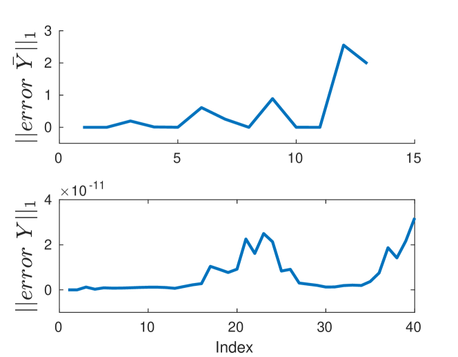
Figure 2: The errors in the observer Markov parameters $\bar{Y}$ for $q=4$, and the open-loop Markov parameters $Y$ calculated on a 3-DoF Spring Mass system used in [9]. The plotted errors are normalized by the true values and the 1-norm of the two channels is calculated. Error $Y$ is the error between the true open-loop Markov parameters of the system and the calculated open-loop parameters from the OKID algorithm. The error $\bar{Y}$ is the error between the estimated ARMA parameters ($\bar{Y}=Z_{t}V^{\dagger}$) and the observer Markov parameters reconstructed from the $\hat{A},\hat{B},\hat{C},\hat{D},\hat{M}$ resulting from the OKID algorithm. The takeaway from this experiment is that the open-loop Markov parameters and the calculated $\hat{A},\hat{B},\hat{C},\hat{D}$, match the true system, but the calculated observer $\hat{M}$ doesn’t explain the ARMA parameters as the reconstructed observer Markov parameters using $\hat{M}$ don’t match the ARMA parameters. We also see that the reconstructed $C\bar{A}^{q}\bar{B}\neq 0$ from the experiment, invalidating the deadbeat assumption.

IV-B Calculation of the open-loop Markov parameters from the ARMA parameters

Restating Eq. (9) for the LTI case:

$$[\alpha_{1}\cdots\alpha_{q}] =CA^{q}(O^{q})^{\dagger}$$

$$[\beta_{1}\cdots\beta_{q}] =([CB,\cdots,CA^{q-1}B]-CA^{q}(O^{q})^{\dagger}G^{q})$$ (27)

Substituting the first equation into the second and rearranging, we get,

$$[CB,\cdots,CA^{q-1}B]=[\beta_{1}\cdots\beta_{q}]+[\alpha_{1}\cdots\alpha_{q}]G^{q}.$$ (28)

Then,

$$Y_{0}:=CB =\beta_{1}+\alpha_{1}D,$$

$$Y_{1}:=CAB =\beta_{2}+\alpha_{1}Y_{0}+\alpha_{2}D,$$

$$Y_{k-1}:=CA^{k-1}B =\beta_{k}+\alpha_{k}D+\sum_{i=1}^{k-1}\alpha_{i}Y_{k-i-1}.$$ (29)

The Markov parameters can be calculated to any length by setting $\alpha_{k}$ and $\beta_{k}$ to $0,\ \forall\ k>q$. The equations used to derive the open-loop Markov parameters from the ARMA parameters are identical to OKID, but they originate from Eq. (5) and (9), which do not require OKID’s hypothesized observer $M$.

Requirements/Issues	TV-OKID	Information-state
ARMA parameters	Yes	Yes
Observability	Yes	Yes
$mq\geq n$	Yes	Yes
$rq\geq n$	Yes	No
Computing open-loop Markov
parameters and Hankel	Yes	No
Experiments to be performed
with zero-initial condition	Yes	No
Free-response experiment	Yes	No
Coordinate transformations	Yes	No
Issue in calculating final $q$ steps	Yes	No

TABLE I: Difference between TV-OKID and Information-state model

IV-C LTV case - Time-varying Observer/Kalman Filter Identification:

The time-varying OKID algorithm (TV-OKID) [11] generalizes the OKID approach by estimating the time-varying ARMA parameters, and goes on to calculate the open-loop Markov parameters from the TV-ARMA parameters. Using the open-loop Markov parameters, ERA is used to calculate $\hat{A}_{t},\hat{B}_{t},\hat{C}_{t}$, and the observer $\hat{M}_{t}=\mathcal{\hat{O}}_{t+1}^{\dagger}P_{k+1}$, where $P_{k+1}$ is a matrix containing the observer gain Markov parameters. The hypothesis is that the calculated system and observer fit the TV-ARMA parameters. The TV-OKID algorithm is complex compared to the time-invariant case, as the calculated $\hat{A}_{t},\hat{B}_{t},\hat{C}_{t},\hat{M}_{t}$ matrices are in a different coordinate system at every time-step $t$. A coordinate transformation has to be performed to bring them to a reference coordinate system [10]. The same issues discussed in the time-invariant case were seen in the time-varying case as well. The Markov parameters of the observer system do not match the TV-ARMA parameters. In addition to needing more computational steps to construct the model, it also requires the experiments to be carried out strictly from zero-initial conditions. In addition to that, another free-response experiment, which involves collecting responses of the system from random non-zero initial conditions with zero forcing, has to be performed to identify models for the first few time-steps and the last few time-steps. Finally, the last $q$ steps cannot be identified for finite-time problems, as the response has to be recorded for $q$ steps after the final time interval.
The Information-state based model doesn’t suffer from any of the above mentioned issues. It is simple, as the state-space model can be arrived at, immediately after calculating the TV-ARMA parameters, courtesy of the information-state. On the other hand, the TV-OKID has to compute the open-loop Markov parameters, build the Hankel matrix to calculate $\hat{A}_{t},\hat{B}_{t},\hat{C}_{t}$, and then transform them to a common reference coordinate system. For prediction, the initial condition has to be explicitly reconstructed after collecting observations in the first $q$ steps, for which it relies on observability - which the information-state model is inherently built upon. The additional requirements and issues pertaining to TV-OKID are tabulated in Table I.
The objective of OKID/TV-OKID to find the open-loop parameters from the ARMA parameters might have been influenced from the traditional Kalman-Ho realization/ ERA procedure and the conventional definition of the state. In essence, the open-loop parameters model the impulse response/forced response, while, the ARMA captures both the initial condition response and the forced response, after an initial transient. The method used to calculate the open-loop parameters from ARMA parameters, strips away the initial condition response to arrive at the impulse response parameters. This is overcome in our method, by using the information-state and constructing the state-space model directly from the ARMA parameters.

V Empirical Results

We tested the information-state technique on the oscillator system used in [10, 11] and on the cart-pole and fish systems available in the open-source MuJoCo simulator [16]. The details of the systems are given in Table II. While the oscillator system is a true LTV system, the cart-pole and the fish are nonlinear systems.

(a)

(b)

Figure 3: Models simulated in MuJoCo.

System	Horizon	$q$	State	Output	Input
			dim. ($n$)	dim. ($m$)	dim. ($r$)
3 DoF Spring-
mass (LTI) [9]	40	4	6	2	1
Oscillator [10]	30	4	4	2	2
Cart-pole	31	4	4	2	1
Fish	30	5	27	11	6

TABLE II: Simulation details

For the oscillator, the identification is straightforward. The system was perturbed with random inputs from a normal distribution and the corresponding output responses were recorded. For nonlinear systems, the system identification has to be carried out along a trajectory about which the system can be linearized. Given a nonlinear system of the form $x_{t+1}=F(x_{t},u_{t}),\ z_{t}=C_{t}x_{t}+D_{t}u_{t}$, it can be linearized along a trajectory $\{\bar{x}_{t},\bar{u}_{t}\}^{T}_{t=0}$. The resulting LTV system is given by: $\delta x_{t+1}\approx A_{t}\delta x_{t}+B_{t}\delta u_{t}$, where $\delta x_{t}=x_{t}-\bar{x}_{t}$, $\delta u_{t}=u_{t}-\bar{u}_{t}$ and $A_{t}=\frac{\partial F}{\partial x}|_{\bar{x},\bar{u}}$ , $B_{t}=\frac{\partial F}{\partial u}|_{\bar{x},\bar{u}}$. And, $\delta z_{t}=C_{t}\delta x_{t}+D_{t}\delta u_{t}.$ The nominal trajectory was computed using the iLQR algorithm [17] and the perturbed system is identified around that trajectory using the input-output responses for every $t$ from $N$ independent experiments/rollouts $\{\delta u_{t}^{(1:N)},\delta z_{t}^{(1:N)}\}$.
Using the input-output responses from the experiments, the TV-ARMA parameters were estimated, from which the information-state based state-space model (Eq. (16)) is constructed. TV-OKID was also implemented to compare its performance. In addition to the forced response experiment, TV-OKID requires a free-response experiment. So, a set of random initial conditions are taken for the system under consideration, and the unforced responses are recorded to identify the system matrices for the first $q$ steps. TV-OKID algorithm computes the system matrices $\hat{A}_{t},\hat{B}_{t},\hat{C}_{t},\hat{D}_{t},\hat{M}_{t}$ from the TV-ARMA parameters and the free-response experiment, using the procedure discussed in [11]. The initial state is estimated using the observations from the first $q$ steps. In order to empirically test the performance of TV-OKID and its inherent observer in the loop hypothesis, we plot two responses: one with the observer in the loop, and one without. The state is propagated using the system matrices and the observer in the first response. The inputs to this observer in the loop system are the control input $u_{t}$ and the true observation $z_{t}$ recorded at that time-step. We also plot the response of the system without including the observer (labeled TV-OKID (without obs.)), to show its performance. For the oscillator, two experiments were performed - one with zero-initial conditions and another with non-zero initial conditions and the results are shown in Fig. 4. The results for the nonlinear systems are shown in Fig 5. The error shown in the figures is the 1-norm of the mean error between true response and the predicted response from 100 independent simulations, across all the output channels.

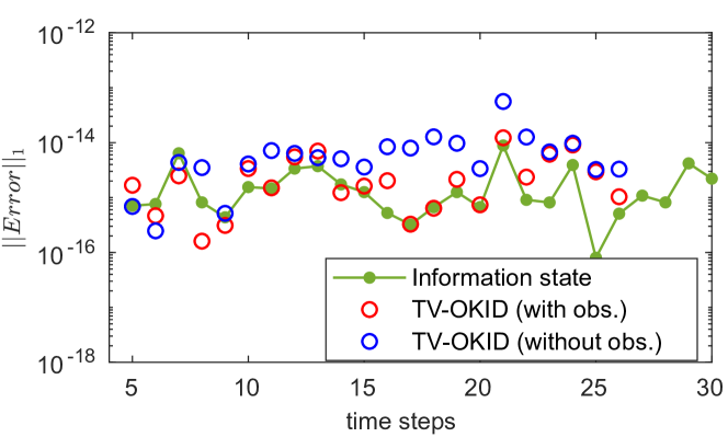
(a) Model calculated using responses from zero initial conditions

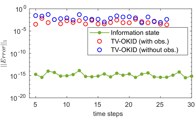
(b) Model calculated using responses from non-zero initial conditions

Figure 4: Results on the oscillator model. OKID requires the data used for identification to have zero-initial conditions, to calculate the first few Markov parameters accurately. The plot ‘TV-OKID (without obs.)’ uses the identified $\hat{A}_{t},\hat{B}_{t},\hat{C}_{t},\hat{D}_{t}$ matrices for prediction, without the observer $\hat{M}_{t}$ in the loop.

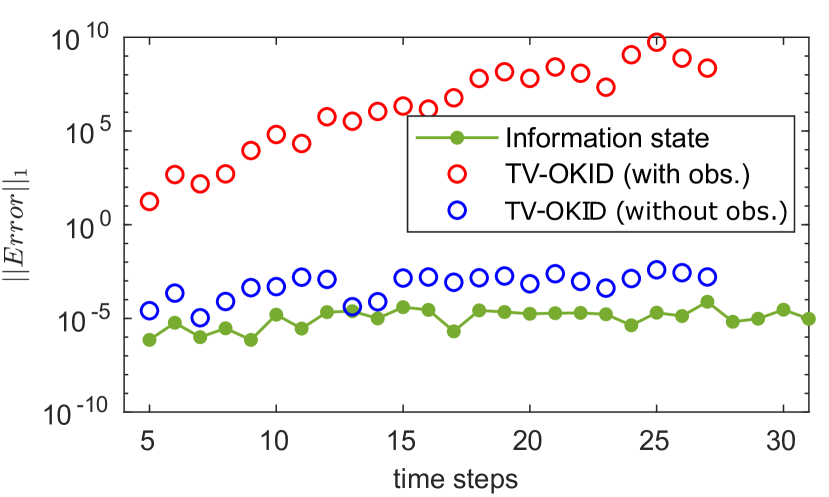
(a) Cart-pole

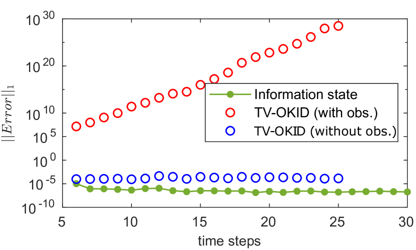
(b) Fish

Figure 5: Results on the nonlinear models. The experiments for identifying the system were performed from zero-initial conditions. The identified observer in both cases is sensitive. Even small errors between the true response and the predicted response in the first few steps are amplified, leading to instability.

The results show that the information-state model can predict the responses accurately. The TV-OKID approach also can predict the response well for both the observer in the loop and without in the oscillator experiment, when the experiments have zero initial conditions, but it suffers from inaccuracy if the experiments have non-zero initial conditions as seen in Fig. 4b. It also fails with the observer in the loop when used for the cart-pole and the fish systems. We found that albeit the identified open-loop Markov parameters predict the response well, when the observer is introduced, the prediction diverges from the truth, further validating the hypothesis that the ARMA model cannot be explained by an observer in the loop system. The last $q$ steps in OKID are ignored, as there is not sufficient data to calculate models for the last few steps, as discussed in sec. IV-C. There is also the potential for numerical errors to creep in due to the additional steps taken in TV-OKID: determination of the time varying Markov parameters from the time varying observer Markov parameters, calculating the SVD of the resulting Hankel matrices and the calculation of the system matrices from these SVDs, as mentioned in [11]. On the other hand, the effort required to identify systems using the information-state approach is negligible compared to other techniques as the state-space model can be set up by just using the ARMA parameters. More examples can be found in [1], where the authors use the information-state model for optimal feedback control synthesis in complex nonlinear systems.

VI Conclusion

This paper describes a new system realization technique for the system identification of linear time-invariant as well as time-varying systems. The system identification method proceeds by modeling the current output of the system using an ARMA model comprising of the finite past outputs and inputs. A theory based on linear observability is developed to justify the usage of an ARMA model, which also provides the minimum number of inputs and outputs required from history for the model to fit the data exactly. The method uses the information-state, which simply comprises of the finite past inputs and outputs, to realize a state-space model directly from the ARMA parameters. This is shown to be universal for both linear time-invariant and time-varying systems that satisfy the observability assumption. The method is tested on various systems in simulation, and the results show that the models are accurately identified. Future work will explore on how to account for both process and sensor noise acting on the system, and its implications for whether an accurate model can be estimated without knowledge of the process noise.

References

- [1] Ran Wang, Raman Goyal, Suman Chakravorty and Robert E. Skelton “Data-based Control of Partially-Observed Robotic Systems” In IEEE International Conference on Robotics and Automation (ICRA), 2021, pp. 8104–8110 DOI: 10.1109/ICRA48506.2021.9561001
- [2] Lennart Ljung “System identification” In Signal analysis and prediction Springer, 1998, pp. 163–173
- [3] Jer-Nan Juang “Applied system identification” Prentice-Hall, Inc., 1994
- [4] Jer-Nan Juang and Richard S Pappa “An eigensystem realization algorithm for modal parameter identification and model reduction” In Journal of guidance, control, and dynamics 8.5, 1985, pp. 620–627
- [5] Shahriar Shokoohi and Leonard M Silverman “Identification and model reduction of time-varying discrete-time systems” In Automatica 23.4 Elsevier, 1987, pp. 509–521
- [6] B.. Ho and R.. Kalman “Effective construction of linear state-variable models from input/output functions” In Proceedings of the 3rd Annual Allerton Conference on Circuit and System Theory 14.1-12, 1965, pp. 545–548 DOI: doi:10.1524/auto.1966.14.112.545
- [7] Manoranjan Majji “Time Varying Covariance Equivalent Realizations” In 2018 Annual American Control Conference (ACC), 2018, pp. 283–287 IEEE
- [8] Andrew M King, Uday B Desai and Robert E Skelton “A generalized approach to q-Markov covariance equivalent realizations for discrete systems” In Automatica 24.4 Elsevier, 1988, pp. 507–515
- [9] Jer-Nan Juang, Minh Phan, Lucas G. Horta and Richard W. Longman “Identification of observer/Kalman filter Markov parameters - Theory and experiments” In Journal of Guidance, Control, and Dynamics 16.2, 1993, pp. 320–329 DOI: 10.2514/3.21006
- [10] M. Majji, J. Juang and J.. Junkins “Time-Varying Eigensystem Realization Algorithm” In Journal of Guidance, Control, and Dynamics 33.1, 2010, pp. 13–28 DOI: 10.2514/1.45722
- [11] Manoranjan Majji, Jer-Nan Juang and John L. Junkins “Observer/Kalman-Filter Time-Varying System Identification” In Journal of Guidance, Control, and Dynamics 33.3, 2010, pp. 887–900 DOI: 10.2514/1.45768
- [12] Michel Verhaegen and Xiaode Yu “A class of subspace model identification algorithms to identify periodically and arbitrarily time-varying systems” In Automatica 31.2, 1995, pp. 201–216 DOI: https://doi.org/10.1016/0005-1098(94)00091-V
- [13] Jer-Nan Juang and Minh Phan “Deadbeat predictive controllers”, 1997
- [14] Minh Phan, Lucas G Horta, Jer-Nan Juang and Richard W Longman “Linear system identification via an asymptotically stable observer” In Journal of Optimization Theory and Applications 79.1 Springer, 1993, pp. 59–86
- [15] Panos J. Antsaklis and Anthony N. Michel “Linear systems” New York: McGraw-Hill,, 1997
- [16] Emanuel Todorov, Tom Erez and Yuval Tassa “MuJoCo: A physics engine for model-based control” In 2012 IEEE/RSJ International Conference on Intelligent Robots and Systems, 2012, pp. 5026–5033 DOI: 10.1109/IROS.2012.6386109
- [17] Raman Goyal, Ran Wang, Suman Chakravorty and Robert E. Skelton “Partially-Observed Decoupled Data-based Control (POD2C) for Complex Robotic Systems” In ArXiv 2107.08086, 2022 DOI: 10.48550/ARXIV.2107.08086