Normal Transformer: Extracting Surface Geometry from LiDAR Points Enhanced by Visual Semantics

Abstract

High-quality estimation of surface normal can help reduce ambiguity in many geometry understanding problems, such as collision avoidance and occlusion inference. This paper presents a technique for estimating the normal from 3D point clouds and 2D colour images. We have developed a transformer neural network that learns to utilise the hybrid information of visual semantic and 3D geometric data, as well as effective learning strategies. Compared to existing methods, the information fusion of the proposed method is more effective, which is supported by experiments.

We have also built a simulation environment of outdoor traffic scenes in a 3D rendering engine to obtain annotated data to train the normal estimator. The model trained on synthetic data is tested on the real scenes in the KITTI dataset. And subsequent tasks built upon the estimated normal directions in the KITTI dataset show that the proposed estimator has advantage over existing methods.

Introduction

Decoding interesting 3D geometric information of an environment using observations from a specific viewpoint is challenging. The primary difficulty arises from the inherent insufficiency of information to capture a 3D scene from one viewpoint. For example, image pixels lack depth information and are subject to perspective ambiguity. On the other hand, in a point cloud, individual points contain the distance to the ego-device in 3D space. The neighbourhood of points could help estimate the local geometry of the object surface. However, the 3D points are unorganised. The topological and geometrical information of the surfaces is not directly available.

Surface normal has proven helpful for many 3D computer vision applications such as reconstruction (Kazhdan, Bolitho, and Hoppe 2006), point cloud registration (Pomerleau, Colas, and Siegwart 2015), scene rendering (Kovac and Zalik 2010), etc. In the context of self-driving, point clouds with accurate normal vectors can provide richer information for understanding urban environments’ internal spatial relationships. Compared to the raw point cloud, the mid-level surface normal prediction can contribute to the interpretability and the reliability of performing the tasks. For example, based on predicted distances to object surface, the decision of performing collision avoidance could be better understood. We consider the problem of estimating the normal vectors of object surface from point clouds. The classical regression-based methods (Hoppe et al. 1992) formulate surface normal estimation as a least-squares optimisation problem. However, traditional methods could easily become fragile in real scenarios because they are sensitive to noise and manually selected parameters. Recently, learning-based techniques have demonstrated promises to outperform traditional methods (Qi et al. 2017a). However, such methods take uniform, dense point clouds from scanned/synthetic objects. They do not apply to more realistic scenarios, such as the LiDAR scans in autonomous driving.

In real-life LiDAR scans, the points are distributed unevenly. One of the major challenges in geometry reconstruction is the scarcity of scan points in areas of interest, especially in middle/long-range fields. The scan becomes sparser with growing distance from the device and often leaves broken/missing surfaces. On the other hand, an image is an observation of a high-resolution dense pixel array of the scene. Such images also imply the scene geometry – biological and machine vision can perform effective geometric inference from images. Therefore, our motivation is to utilise the rich semantic information in images to assist the recovery of surface normal directions from point clouds.

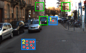
Figure 1: Semantic information in related regions can help estimate surface normals. The figure shows estimation of normal in two regions R-1: faraway, R-2: near. R-1 is more challenging due to sparse 3D points. The estimation can be assisted by visual information in close/related regions (light green boxes).

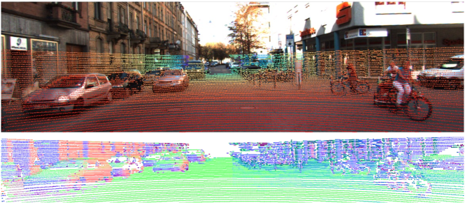
Figure 2: Normal estimation on KITTI data. (top) LiDAR scans projected to images. (bottom) Surface normal estimated by Hybrid Geometry Transformer.

The normal of a point on a smooth surface is directly determined by a small neighbouring area. Theoretically, one only needs to collect sufficient points of a small region around a point ${\boldsymbol{x}}$ to recover the corresponding normal vector ${\boldsymbol{v}}^{(x)}$. In practice, the sensory data can be scarce at some point. Hence it is helpful to exploit cues from regions related to the target point ${\boldsymbol{x}}$, where those regions may or may not immediately touch ${\boldsymbol{x}}$. The relationship could be of high level and has semantic meaning, and is to be discovered through learning-based methods.

Figure 1 shows an example of the proposed method. The masked region 1 and 2 are both road surfaces (transparent light blue in the figure). R-2 is close to the device. And given a small area in R-2, the LiDAR points falling in the area are multitude. The surface geometry could be directly computed using the points. On the other hand, R-1 is faraway. The points are sparse. At one location in R-1, a small neighbourhood may contain only one or a few points. No reliable geometric information can be directly extracted from the small set of scan points. However, if one considers the image regions marked by green boxes, the geometry in R1 could be implied by the visual information:

Q: ”What could be a flat surface lying between two buildings and supporting a vehicle beside it?”

A: ”Perhaps a patch of road.”

A naive approach would be adopting convolutional operators to extract local features from the sensory data to represent relevant geometric information, including variants of sparse or graph-based local operators (Yan, Mao, and Li 2018; Pareja et al. 2020). However, determining the scale of a “local” area at every point on a manifold is a non-trivial task. And manually crafted procedures also tend to be fragile to deal with complex geometric structures.

To automatically identify and utilise relevant information in the sensory data, this work presents the following insights and innovations:

• We present a transformer neural network-based model, Hybrid Geometry Transformer (HGT), to extract geometric information and estimate normal directions from hybrid data (Figure 2).

• We propose an effective training technique for self-attention nets on large-scale outdoor data.

• We release a data collection toolkit for the Urban environment built on the Unity 3D platform.

• The evaluation results show that HGT outperforms previous methods. Furthermore, the tests on KITTI benchmark reveal that our method has excellent generalisation.

Related Work

Normal estimation is an essential task in 3D scene understanding. The simplest and best-known approach is to fit a least-squares local plane using principal component analysis (PCA) (Hoppe et al. 1992). Although this method is efficient and well-understood, it is sensitive to noise and density variations and tends to smoothen sharp details (Mitra, Nguyen, and Guibas 2004). To address these challenges, some techniques were proposed to achieve more robust estimation, such as Voronoi cells (Amenta and Bern 1999; Alliez et al. 2007; Mérigot, Ovsjanikov, and Guibas 2011), distance-weighted approaches (Pauly et al. 2003) and algebraic spheres’ fitting (Guennebaud and Gross 2007). 3F2N (Fan et al. 2020) is a fast and accurate normal estimator performing three filtering operations on an inverse depth or a disparity image. However, both these traditional methods still depend heavily on the hyper-parameters like neighbourhood size.

Researchers have applied data-driven deep neural networks widely in the field of 3D shape analysis. In particular, we can group models presented for normal estimation into several categories depending on the data sources.

Based on Image: This kind of work takes a single depth/colour image or both as input and then performs the pixel-wise normal estimation. For a single RGB image, Eigen et al. (Eigen, Puhrsch, and Fergus 2014) designed a three-scale convolution network to produce better results than traditional methods. Bansal et al. (Bansal, Russell, and Gupta 2016) and Zhang et al.(Zhang et al. 2017) adopted the skip-connected structure and U-Net structure to improve performance. Very recently, GeoNet (Qi et al. 2018) and GeoNet++ (Qi et al. 2020) use two-stream CNNs to predict both depth and surface normal maps from a single RGB image. Some works utilise both depth and RGB images (C. et al. 2013; Gong et al. 2013; Liu, Gong, and Liu 2012). Recently, Zeng et al. (Zeng et al. 2019) presented a hierarchical fusion scheme for RGB-D data in a deep learning model and reached state-of-the-art performance.

The common challenge for these image-based methods is the low data efficiency, which means the training procedure requires a large amount of labelled surface normals (Li et al. 2015). In contrast, the point-based approach can improve data efficiency due to the explicit use of intrinsic 3D structure in supervised learning.

Based on Point Cloud: Another group of methods perform 3D scene understanding with point cloud only. Those methods usually use PointNet backbone (Qi et al. 2017a) or Graph neural networks (GNNs) (Wu et al. 2021) to handle unstructured 3D points. Earlier attempts on normal estimation task came from (Guerrero et al. 2018). They use PointNet architecture to extract local 3D shape properties from multi-scale patches of a point cloud. (Ben-Shabat, Lindenbaum, and Fischer 2019) designed an extra module that learns to decide the optimal scale and hence improves performance. The recent method presented by (Lenssen, Osendorfer, and Masci 2020) uses GNNs to model an adaptive anisotropic kernel that iteratively produces point weights for weighted least-squares plane fitting.

It is worth mentioning that the point cloud data used above is mainly gathered from small CAD objects or indoor depth cameras. These point clouds have an even and relatively high density. But In outdoor scenes like urban environments, The heavy interference of the passive illumination (Fanello et al. 2017) usually makes those active depth sensing solutions fail. In distant areas with low resolutions and small triangulation, stereo methods become less accurate. Hence, LiDAR has become the dominating reliable depth solution in the outdoor environment. But LiDAR still has the drawback of being too expensive and having notorious low-resolution (Lingfors et al. 2017). So the point cloud gathered from LiDAR is generally sparse, with noise and a nonuniform point density. Due to the limitations of LiDAR data and the complexity in an outdoor environment, approaches suitable for a dense indoor dataset are often incapable of estimating accurate normals for outdoor data.

Based on colour Image and Sparse LiDAR scans: Few investigations have looked into estimating normal from image and sparse point cloud. Most related to this field, DeepLiDAR (Qiu et al. 2019) uses LiDAR projection maps and images as input and then feeds them into a CNN-based encoder-decoder for normal estimation.

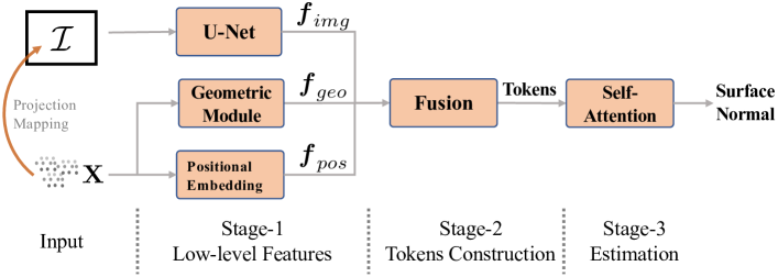
Figure 3: Diagram of the pipeline of estimating normal from image and LiDAR points.

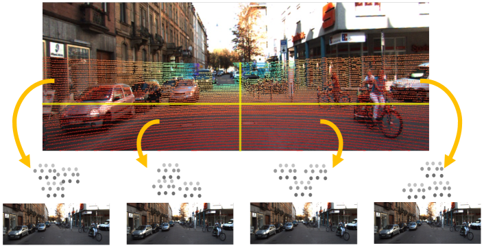
Figure 4: Making small sample by partitioning point clouds. The LiDAR points are grouped by the projections on the image into 4 panes. Note the entire image is associated with each group of the points to make the input sample, not only the visual contents in the corresponding pane.

Method

In this section, we present the proposed framework to estimate normal directions on 3D points from hybrid observation of LiDAR point clouds and images. The computational model is derived from the attention transformers.

Figure 3 shows the workflow of the framework. The input data consist of two parts: an image $\mathcal{I}$ and a point cloud $\mathbf{X}$, where $\mathbf{X}$ is an $[N\times 3]$ array containing the coordinates of a set of 3D points. The point cloud is a subset of raw LiDAR scans. Each point within it has a projection on the image. The desired output of the model is the surface normal vectors at points in $\mathbf{X}$. The relative pose of the LiDAR device and the camera is known. Image and geometric features are extracted from $\mathcal{I}$ and $\mathbf{X}$, respectively. The features and encoded positions of the points are fed to an attentional transformer to estimate the normal directions at the points.

The details of the computational steps and the learning of the model are discussed in the remaining of this section.

Low-level features

As shown in Figure 3, low-level features are descriptors of the 3D points, carrying three pieces of information: local image content, local point cloud geometry and location.

For each 3D point ${\boldsymbol{x}}_{i}$, a Euclidean neighbourhood, $\mathcal{N}_{i}$, is extracted. The following image and geometric features at the neighbour points will be aggregated to produce a descriptor $\phi({\boldsymbol{x}}_{i})$ at ${\boldsymbol{x}}_{i}$.

$$\phi(x_{i}) \leftarrow R(\{{\boldsymbol{f}}_{j}|j\in\mathcal{N}_{i}\})$$ (1)

$${\boldsymbol{f}}_{j} \leftarrow G({\boldsymbol{f}}_{img}(j)\oplus{\boldsymbol{f}}_{geo}(j)\oplus{\boldsymbol{f}}_{pos}(j))$$ (2)

where $R$ is an operator of a reduction, aggregating the features ${\boldsymbol{f}}$ at the neighbour points. A feature vector is the result of fusing (e.g. using a MLP $G$) three-component features: i) image feature, ${\boldsymbol{f}}_{img}$, ii) geometric feature ${\boldsymbol{f}}_{geo}$ and iii) encoded positions ${\boldsymbol{f}}_{pos}$. The image and geometric features are derived from widely applied techniques as follows.

The image features are computed at each image pixel using a U-Net fully convolutional structure (Ronneberger, Fischer, and Brox 2015). The U-Net is known for its capability to extract locally semantic information from an image. The hourglass structure enables the net to utilise the information at multiple scales to make predictions. The attribute is desirable for the motivation of utilising semantics to make the normal estimation more robust.

The geometric features at 3D points are computed using an MLP structure derived from the PointNet++ (Qi et al. 2017b). At each 3D point $\boldsymbol{x}_{i}$, the feature vector is computed using an MLP shared by all points.

The location of a point is encoded by positional embedding layers, which employ MLP structures as well. Following the common practice of encoding 2D coordinates in image processing (Dosovitskiy et al. 2021), we encode every point’s 3D spatial information in the global coordinate system.

Transformer Encoder and Prediction Head

After low-level feature extraction in (2), the model constructs tokens ${\mathbf{T}}:[N\times D]$ that will then be passed into a transformer encoder with multiple self-attention layers. In each layer, ${\mathbf{T}}$ is linearly transformed into three tensors ${\mathbf{Q}}$, ${\mathbf{K}}$, and ${\mathbf{V}}$. Then ${\mathbf{Q}}$ and ${\mathbf{K}}$ are used to represent the relationship between the tokens. One commonly adopted computational model of the relation is to take the inner product:

$${\mathbf{A}}=\text{Norm}({\mathbf{Q}}{\mathbf{K}}^{T})$$ (3)

where Norm means normalisation operation (Guo et al. 2021) over the rows of the matrix ${\mathbf{A}}\in\mathbb{R}^{N\times N}$. The entry $A_{i,j}$ represents how token $i$ in ${\mathbf{Q}}$ is related to the reference token $j$ in ${\mathbf{K}}$ and ${\mathbf{V}}$.

The model then conducts a matrix multiplication ${\mathbf{A}}{\mathbf{Q}}$ for internal feature combinations between tokens. The combined tokens are passed into a batch normalisation and residual connection. Finally, the layer outputs new tokens ${\mathbf{T}}^{\prime}$ serving as the next self-attention block’s input. More details can be found in the appendix.

Following the transformer encoder, an MLP prediction head transforms each encoded token into a 3-dimensional vector representing three components of the surface normal. Finally, we regularise the output to unit 3D vectors to ensure a reasonable surface normal.

Loss function

The loss function for optimising the neural network model is defined as the mean squared error (MSE) between the directions of the predicted and the ground-truth normal vectors. The MSE of the predictions at $N$ points is

$$\mathcal{L}=\frac{1}{N}\sum_{j}^{N}\|\hat{\boldsymbol{v}}_{reg}^{(j)}-\boldsymbol{v}_{gt}^{(j)}\|_{2}^{2}$$ (4)

where $\hat{\boldsymbol{v}}_{reg}^{(j)}$ is the prediction normalised to unit length and $\boldsymbol{v}_{gt}^{(j)}$ is the ground-truth normal vector.

Effective Training of the Attentional Transformer

Batching

The transformer normal estimator is designed to utilise semantic information across the scene by employing large attentional fields. However, the attention model is expensive in terms of computation and storage. The attention weight matrix ${\mathbf{A}}\in\mathbb{R}^{N\times N}$ in (3) grows quadratically with the fused features, which is prohibitive for a complex scene.

More specifically, fully executing the model on one typical training sample ($400\times 400$ image and  10K points) costs about 6 Gigabytes of GPU memory. The cost is about 4x higher for a single frame in the real traffic scene in the KITTI dataset. Although straightforward implementation is viable on modern hardware configurations, the sample number in a batch during training must be compromised. At the same time, the batch size can affect the effectiveness of training (Santurkar et al. 2018).

For effective training, we partition the point cloud in one frame by grouping the points according to their projections on the image. For example, Figure 4 (a) shows partitioning the points into 4 parts. The points of each part make one training sample. Since the input tokens of the transformer net correspond to individual points, the partitioned samples make the size of the weight matrix ${\mathbf{A}}$ decreases quadratically, e.g. from $[N\times N]$ to $[\frac{1}{4}N\times\frac{1}{4}N]$ in the example shown in Figure 4. Within the storage limit, the batch size can be increased correspondingly, see the right pane of the figure. Increased batch is helpful during the training, especially when batch normalisation is employed.

In this paper, we use $\frac{1}{16}$ of each frame’s point cloud, and the batch size is 8. The experimental results in Figure 12 show that our training technique will not lead to a loss of global sensibility during the testing phase. Furthermore, this technique can also be used in the testing phase if the range of scene observation is too extensive.

Synthetic data

Measuring normal directions is difficult in practical applications. And most real-world datasets do not contain annotations of the ground-truth normal directions. A toolkit is developed to produce synthetic data by simulating a city scene in a realistic 3D renderer environment. Artificial cameras and LiDAR devices are planted in the scene. We construct a customised shader to synthesise the normal vectors at points on object surfaces. Data samples are collected in the same form as the actual sensors. More importantly, labels (colours, depth, surface normals) are easily acquired from the simulator. Details about how data is synthesised can be found in the next section. We use this dataset to train and evaluate our model.

Experiments have shown that the model trained only on synthetic data has been able to generalise to practical datasets and obtain impressive results. Further improvement could be achieved if we use real-world data to fine-turn our model.

Experiments

This section presents the experiment results of the proposed technique. We first introduce how the synthetic data has been constructed. We then evaluate our model on this dataset and compare it with other existing works. We add different levels of noise into the data to test whether our model is robust. The model trained on the synthetic dataset is also applied to the real-life KITTI dataset (Geiger et al. 2013). The KITTI dataset does not contain ground-truth normal directions at the LiDAR points. Hence the estimated normal directions are used for 3D reconstruction to assess the estimation.

Data Synthesis

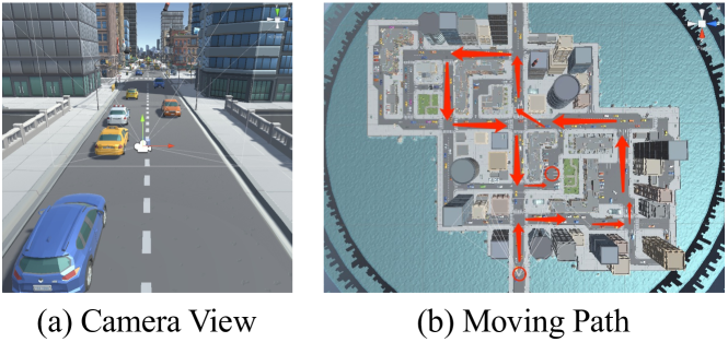
Figure 5: Scene and movement setup for data collection.

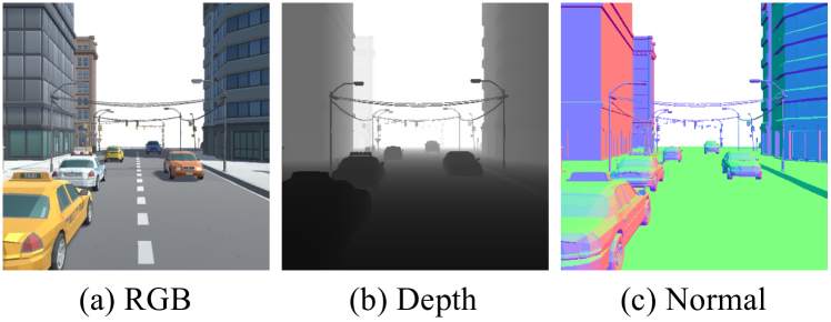
Figure 6: Observations rendered by shaders in the 3D rendering engine.

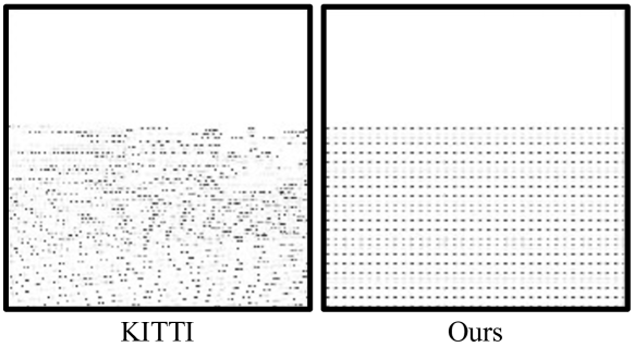
Figure 7: LiDAR points’ projection of KITTI and our synthetic data.

We exploit Unity 3D (Haas 2014) as a simulator and rendering engine to collect data. We first build a high-quality outdoor scene, which contains vehicles, cyclists, pedestrians, and necessary lighting configurations. The details are in the appendix. The scene can be easily changed to others according to practical needs. Our efforts mainly focus on the data collection after setting up a scene. More specifically, we develop in the following aspects.

Sensors and Shaders: The sensors we place in the simulator include a colour camera, depth camera and normal sensor. The depth sensor is utilised to produce LiDAR points in the latter process. As shown in Figure 5 (a), we place these sensors on the roof of the car. We can render the sensor observations by developing engine shaders for the three sensors, as shown in Figure 6.

LiDAR acquisition: We find that the LiDAR projections to the image are mostly uniform. Therefore we take the lower rectangular region of the image and evenly sample rays passing through the image pixels to simulate projected LiDAR points. Note the points are distributed evenly on the image, but not in the 3D scene. The density has been made comparable to that in the KITTI dataset. Figure 7 compares the sampling of the LiDAR points between the synthetic and KITTI datasets.

We then apply the designed mask to the given depth map from the sensor. Finally, the synthetic LiDAR scans can be obtained via inverse projection using camera intrinsic. Unlike other simulators, which spend a lot of time and computational cost on simulating real LiDAR using ray tracing, we simulate LiDAR directly from the depth map.

Dataset generation: With the communication interfaces provided by ML-Agent (Juliani et al. 2018), we deploy scripts in Unity and an external Python-based controller, respectively. The complete pipeline is discussed in appendix.

We follow the preset path shown in Figure 5 (b) and collect $151$ frames’ observations ($121$ for training, $30$ for testing), which contain images with size $400\times 400$, sparse LiDAR points in view, and points’ surface normal ground truth. For convenience, we export the projection relationship arrays between LiDAR points and pixel index and the camera projection matrix.

To evaluate the robustness of the model, we also add different levels of noises to the LiDAR data. Note that we only add a numerical drift to the $z$-coordinate (in front of the camera) of the LiDAR point cloud. The noises follow the settings in (Ben-Shabat, Lindenbaum, and Fischer 2019; Guerrero et al. 2018), see Figure 8.

Implementation Details

We implement our model using PyTorch (Paszke et al. 2019) on a NVIDIA RTX 5000 GPU. We adopts Adam (Kingma and Ba 2015) as optimiser with learning rate $1e^{-4}$, $\beta_{1}=0.9$, $\beta_{2}=0.999$. All models are trained for $200$ epochs from randomly initialised parameters.

In the low-level features extraction, for each point, we randomly select $60$ neighbours, and the radius of the spherical query is $0.75$. If there are fewer points within the sphere, we will pad the results with the querying point itself. The neural networks are introduced in the appendix. The transformer contains three self-attention blocks.

Test on Synthetic Data

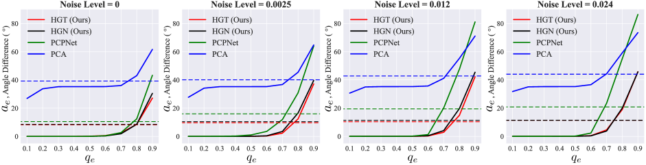
Figure 8: Error distributions on the synthetic dataset. The horizontal axis ($q_{e}$) represents the error quantiles. The vertical axis represents the angle difference $a_{e}$. Lower $a_{e}$ arises later along $q_{e}$ means more accurate predictions. Solid lines in different colours correspond to different techniques under test. The broken lines represent the average error for each method. The panes correspond to different noise levels.

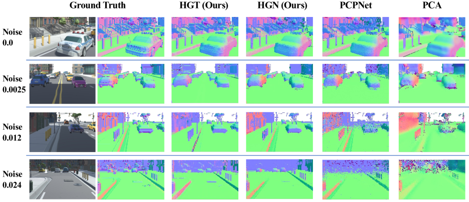
Figure 9: Qualitative Comparison on synthetic dataset

Method	Noise Level
	0	0.0025	0.012	0.024
PCA	39.27	40.10	42.80	44.06
PCPNet	10.50	15.94	19.50	20.83
HGN (Ours)	8.49	10.42	11.31	11.41
HGT (Ours)	8.18	9.61	10.36	11.38

Table 1: Average angle error on synthetic dataset. The comparison include PCA (Hoppe et al. 1992), PCPNet (Guerrero et al. 2018) and our method. The HGN (Hybrid Geometry Network) removes the transformer structure from our final model HGT for ablation study.

Evaluation Metric

To compare two directions, we consider directly measure the angles between the vectors. The following trigonometric evaluation is computed.

$$d_{angle}=\frac{1}{N}\sum_{j}^{N}\arccos(\frac{\lvert\hat{\boldsymbol{v}}_{reg}^{(j)}\cdot\boldsymbol{v}_{gt}^{(j)}\rvert}{\lvert\hat{\boldsymbol{v}}_{reg}^{(j)}\rvert\lvert\boldsymbol{v}_{gt}^{(j)}\rvert})$$ (5)

The angle difference is consistent with MSE.

Performance

Figure 8 compares the prediction accuracy of HGT and existing methods. Specifically, the points are sorted by the estimation errors at each of them in ascending order. For example, the location of $0.5$ on the horizontal axis represents the median of the prediction error. The figure shows HGT is robustly outperforming existing techniques at different noise levels and at all quantiles of error distribution. Table 1 lists the average errors for a numerical comparison, the numbers corresponding to the broken lines in Figure 8.

The results demonstrate that our method can produce lower error estimates. Besides, our method is more robust to LiDAR noise. The error only increases slightly as the noise change from $0$ to $0.024$. In Figure 8, we noticed that the tail of the error distribution is in a high value, which leads to a large mean error and smaller gaps between different methods. We found that these high error estimations appeared in regions like wires and object edges, where normal directions are difficult to extract and have minimal significance. Figure 9 further visualises some of the estimated surface normal maps for qualitative comparison. The full results are included in the appendix. We find that HGT has significant advantages in finely structured objects such as ladders.

The report does not include the results of DeepLiDAR (Qiu et al. 2019) since its pure CNN-Based architecture can not converges well on our small dataset (only $121$ images and point clouds). This also reveals that our hybrid structure is more effective in handling multi-modal data.

Generalisation Test on KITTI

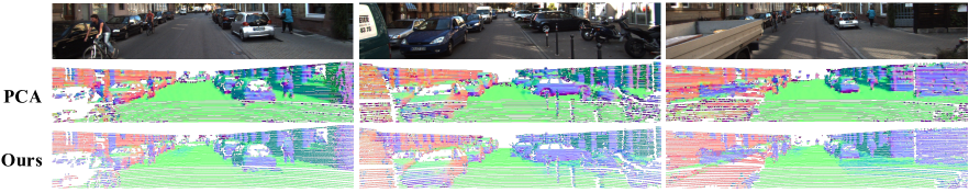
Figure 10: Qualitative results on KITTI.

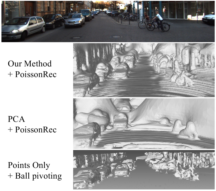
Figure 11: Test on scene reconstruction task.

We use the real-world dataset KITTI (Geiger et al. 2013) in this experiment to investigate the model generalisation. Given a frame of LiDAR scans and camera observations of KITTI, we first compute and save the point-to-pixel projection mapping with calibration parameters provided by the dataset. Then we feed the KITTI frames into the model trained on synthetic data without any fine-turn.

For comparison, we also illustrate the surface normal map produced by the classical PCA used in DeepLiDAR (Qiu et al. 2019) for normal reconstruction. The results are shown in Figure 10. The full results are included in the appendix. HGT has generalised surprisingly well given the fact that no fine-tuning has been conducted on the KITTI dataset. Compare the estimated normal directions of the road surface in Figure 9 for a specific example.

Application on 3D Reconstruction

Given the estimated normal directions at the LiDAR points, we perform Poisson Reconstruction (Kazhdan, Bolitho, and Hoppe 2006) on the KITTI dataset. The 3D reconstruction could serve as an intuitive criterion to compare the normal estimation methods. We also include comparisons to reconstruction w/o normals.

As shown in Figure 11, the point-only method can lead to many mesh holes and is unsuitable for handling practical sparse LiDAR data. The Poisson Reconstruction technique can recover a continuous surface with the help of surface normals. By comparison, we can find that our model has a tremendous normal estimation because the quality of the recovered model is highly dependent on the precision of the surface normals.

Additional Experiments

Figure 12: Headmap visualisation of self-attention weight.

Ablation of transformer structure

To investigate how the transformer structure helps to recover the surface normal, we replace self-attention blocks with a PointNet structure. Specifically, an MLP and max pooling operation is applied to tokens and then generates a global feature. We concatenate this global feature to all tokens and pass them to the prediction head. The ablation results can be found in Figure 8 and 9, revealing that the transformer does bring a performance improvement.

Attention behavior visualisation

One of our arguments is to estimate a position’s surface normal using Non-immediately surrounding regions. One common way to verify whether the transformer can implement this is by visualising the attention map inside the trained network. We draw the first self-attention weight matrix ${\mathbf{A}}$ as in Figure 12.

The visualisation results show that each position’s computation has been connect to interested areas over the whole observation. We can easily find that there is a semantic basis for such connections.

Conclusion

We have presented HGT, a transformer-based model that estimates surface normals from image and sparse LiDAR scans. We release a toolkit for data collection and a batching technique that enable effective training. Multiple evaluations show that our model can achieve superior performance on both synthetic and real-world data. A limitation of HGT is that the prediction is at where the LiDAR point is available. In future developments, it can be considered to predict surface normals and other geometric quantities at arbitrary positions.

References

- Alliez et al. (2007) Alliez, P.; Cohen-Steiner, D.; Tong, Y.; and Desbrun, M. 2007. Voronoi-based variational reconstruction of unoriented point sets. In Proceedings of the Fifth Eurographics Symposium on Geometry Processing, Barcelona, Spain, July 4-6, 2007, volume 257 of ACM International Conference Proceeding Series, 39–48. Eurographics Association.
- Amenta and Bern (1999) Amenta, N.; and Bern, M. W. 1999. Surface Reconstruction by Voronoi Filtering. Discret. Comput. Geom., 22(4): 481–504.
- Bansal, Russell, and Gupta (2016) Bansal, A.; Russell, B. C.; and Gupta, A. 2016. Marr Revisited: 2D-3D Alignment via Surface Normal Prediction. In 2016 IEEE Conference on Computer Vision and Pattern Recognition, CVPR 2016, Las Vegas, NV, USA, June 27-30, 2016, 5965–5974. IEEE Computer Society.
- Ben-Shabat, Lindenbaum, and Fischer (2019) Ben-Shabat, Y.; Lindenbaum, M.; and Fischer, A. 2019. Nesti-Net: Normal Estimation for Unstructured 3D Point Clouds Using Convolutional Neural Networks. In IEEE Conference on Computer Vision and Pattern Recognition, CVPR 2019, Long Beach, CA, USA, June 16-20, 2019, 10112–10120. Computer Vision Foundation / IEEE.
- C. et al. (2013) C., D. H.; Kannala, J.; Ladicky, L.; and Heikkilä, J. 2013. Depth Map Inpainting under a Second-Order Smoothness Prior. In Image Analysis, 18th Scandinavian Conference, SCIA 2013, Espoo, Finland, June 17-20, 2013. Proceedings, volume 7944 of Lecture Notes in Computer Science, 555–566. Springer.
- Dosovitskiy et al. (2021) Dosovitskiy, A.; Beyer, L.; Kolesnikov, A.; Weissenborn, D.; Zhai, X.; Unterthiner, T.; Dehghani, M.; Minderer, M.; Heigold, G.; Gelly, S.; Uszkoreit, J.; and Houlsby, N. 2021. An Image is Worth 16x16 Words: Transformers for Image Recognition at Scale. In 9th International Conference on Learning Representations, ICLR 2021, Virtual Event, Austria, May 3-7, 2021. OpenReview.net.
- Eigen, Puhrsch, and Fergus (2014) Eigen, D.; Puhrsch, C.; and Fergus, R. 2014. Depth Map Prediction from a Single Image using a Multi-Scale Deep Network. In Advances in Neural Information Processing Systems 27: Annual Conference on Neural Information Processing Systems 2014, December 8-13 2014, Montreal, Quebec, Canada, 2366–2374.
- Fan et al. (2020) Fan, R.; Wang, H.; Xue, B.; Huang, H.; Wang, Y.; Liu, M.; and Pitas, I. 2020. Three-Filters-to-Normal: An Accurate and Ultrafast Surface Normal Estimator. CoRR, abs/2005.08165.
- Fanello et al. (2017) Fanello, S. R.; Valentin, J. P. C.; Rhemann, C.; Kowdle, A.; Tankovich, V.; Davidson, P. L.; and Izadi, S. 2017. UltraStereo: Efficient Learning-Based Matching for Active Stereo Systems. In 2017 IEEE Conference on Computer Vision and Pattern Recognition, CVPR 2017, Honolulu, HI, USA, July 21-26, 2017, 6535–6544. IEEE Computer Society.
- Geiger et al. (2013) Geiger, A.; Lenz, P.; Stiller, C.; and Urtasun, R. 2013. Vision meets robotics: The KITTI dataset. Int. J. Robotics Res., 32(11): 1231–1237.
- Gong et al. (2013) Gong, X.; Liu, J.; Zhou, W.; and Liu, J. 2013. Guided depth enhancement via a fast marching method. Image Vis. Comput., 31(10): 695–703.
- Guennebaud and Gross (2007) Guennebaud, G.; and Gross, M. H. 2007. Algebraic point set surfaces. ACM Trans. Graph., 26(3): 23.
- Guerrero et al. (2018) Guerrero, P.; Kleiman, Y.; Ovsjanikov, M.; and Mitra, N. J. 2018. PCPNet Learning Local Shape Properties from Raw Point Clouds. Comput. Graph. Forum, 37(2): 75–85.
- Guo et al. (2021) Guo, M.; Cai, J.; Liu, Z.; Mu, T.; Martin, R. R.; and Hu, S. 2021. PCT: Point cloud transformer. Comput. Vis. Media, 7(2): 187–199.
- Haas (2014) Haas, J. K. 2014. A history of the unity game engine.
- Hoppe et al. (1992) Hoppe, H.; DeRose, T.; Duchamp, T.; McDonald, J. A.; and Stuetzle, W. 1992. Surface reconstruction from unorganized points. In Proceedings of the 19th Annual Conference on Computer Graphics and Interactive Techniques, SIGGRAPH 1992, Chicago, IL, USA, July 27-31, 1992, 71–78. ACM.
- Juliani et al. (2018) Juliani, A.; Berges, V.; Vckay, E.; Gao, Y.; Henry, H.; Mattar, M.; and Lange, D. 2018. Unity: A General Platform for Intelligent Agents. CoRR, abs/1809.02627.
- Kazhdan, Bolitho, and Hoppe (2006) Kazhdan, M. M.; Bolitho, M.; and Hoppe, H. 2006. Poisson surface reconstruction. In Proceedings of the Fourth Eurographics Symposium on Geometry Processing, Cagliari, Sardinia, Italy, June 26-28, 2006, volume 256 of ACM International Conference Proceeding Series, 61–70. Eurographics Association.
- Kingma and Ba (2015) Kingma, D. P.; and Ba, J. 2015. Adam: A Method for Stochastic Optimization. In 3rd International Conference on Learning Representations, ICLR 2015, San Diego, CA, USA, May 7-9, 2015, Conference Track Proceedings.
- Kovac and Zalik (2010) Kovac, B.; and Zalik, B. 2010. Visualization of LIDAR datasets using point-based rendering technique. Comput. Geosci., 36(11): 1443–1450.
- Lenssen, Osendorfer, and Masci (2020) Lenssen, J. E.; Osendorfer, C.; and Masci, J. 2020. Deep Iterative Surface Normal Estimation. In 2020 IEEE/CVF Conference on Computer Vision and Pattern Recognition, CVPR 2020, Seattle, WA, USA, June 13-19, 2020, 11244–11253. IEEE.
- Li et al. (2015) Li, B.; Shen, C.; Dai, Y.; van den Hengel, A.; and He, M. 2015. Depth and surface normal estimation from monocular images using regression on deep features and hierarchical CRFs. In IEEE Conference on Computer Vision and Pattern Recognition, CVPR 2015, Boston, MA, USA, June 7-12, 2015, 1119–1127. IEEE Computer Society.
- Lingfors et al. (2017) Lingfors, D.; Bright, J. M.; Engerer, N. A.; Ahlberg, J.; Killinger, S.; and Widén, J. 2017. Comparing the capability of low- and high-resolution LiDAR data with application to solar resource assessment, roof type classification and shading analysis. Applied Energy, 205: 1216–1230.
- Liu, Gong, and Liu (2012) Liu, J.; Gong, X.; and Liu, J. 2012. Guided inpainting and filtering for Kinect depth maps. In Proceedings of the 21st International Conference on Pattern Recognition, ICPR 2012, Tsukuba, Japan, November 11-15, 2012, 2055–2058. IEEE Computer Society.
- Mérigot, Ovsjanikov, and Guibas (2011) Mérigot, Q.; Ovsjanikov, M.; and Guibas, L. J. 2011. Voronoi-Based Curvature and Feature Estimation from Point Clouds. IEEE Trans. Vis. Comput. Graph., 17(6): 743–756.
- Mitra, Nguyen, and Guibas (2004) Mitra, N. J.; Nguyen, A. T.; and Guibas, L. J. 2004. Estimating surface normals in noisy point cloud data. Int. J. Comput. Geom. Appl., 14(4-5): 261–276.
- Pareja et al. (2020) Pareja, A.; Domeniconi, G.; Chen, J.; Ma, T.; Suzumura, T.; Kanezashi, H.; Kaler, T.; Schardl, T. B.; and Leiserson, C. E. 2020. EvolveGCN: Evolving Graph Convolutional Networks for Dynamic Graphs. In The Thirty-Fourth AAAI Conference on Artificial Intelligence, AAAI 2020, The Thirty-Second Innovative Applications of Artificial Intelligence Conference, IAAI 2020, The Tenth AAAI Symposium on Educational Advances in Artificial Intelligence, EAAI 2020, New York, NY, USA, February 7-12, 2020, 5363–5370. AAAI Press.
- Paszke et al. (2019) Paszke, A.; Gross, S.; Massa, F.; Lerer, A.; Bradbury, J.; Chanan, G.; Killeen, T.; Lin, Z.; Gimelshein, N.; Antiga, L.; Desmaison, A.; Kopf, A.; Yang, E.; DeVito, Z.; Raison, M.; Tejani, A.; Chilamkurthy, S.; Steiner, B.; Fang, L.; Bai, J.; and Chintala, S. 2019. PyTorch: An Imperative Style, High-Performance Deep Learning Library. In Advances in Neural Information Processing Systems 32, 8024–8035. Curran Associates, Inc.
- Pauly et al. (2003) Pauly, M.; Keiser, R.; Kobbelt, L.; and Gross, M. H. 2003. Shape modeling with point-sampled geometry. ACM Trans. Graph., 22(3): 641–650.
- Pomerleau, Colas, and Siegwart (2015) Pomerleau, F.; Colas, F.; and Siegwart, R. 2015. A Review of Point Cloud Registration Algorithms for Mobile Robotics. Found. Trends Robotics, 4(1): 1–104.
- Qi et al. (2017a) Qi, C. R.; Su, H.; Mo, K.; and Guibas, L. J. 2017a. PointNet: Deep Learning on Point Sets for 3D Classification and Segmentation. In 2017 IEEE Conference on Computer Vision and Pattern Recognition, CVPR 2017, Honolulu, HI, USA, July 21-26, 2017, 77–85. IEEE Computer Society.
- Qi et al. (2017b) Qi, C. R.; Yi, L.; Su, H.; and Guibas, L. J. 2017b. PointNet++: Deep Hierarchical Feature Learning on Point Sets in a Metric Space. In Advances in Neural Information Processing Systems 30: Annual Conference on Neural Information Processing Systems 2017, December 4-9, 2017, Long Beach, CA, USA, 5099–5108.
- Qi et al. (2018) Qi, X.; Liao, R.; Liu, Z.; Urtasun, R.; and Jia, J. 2018. GeoNet: Geometric Neural Network for Joint Depth and Surface Normal Estimation. In 2018 IEEE Conference on Computer Vision and Pattern Recognition, CVPR 2018, Salt Lake City, UT, USA, June 18-22, 2018, 283–291. IEEE Computer Society.
- Qi et al. (2020) Qi, X.; Liu, Z.; Liao, R.; Torr, P. H. S.; Urtasun, R.; and Jia, J. 2020. GeoNet++: Iterative Geometric Neural Network with Edge-Aware Refinement for Joint Depth and Surface Normal Estimation. CoRR, abs/2012.06980.
- Qiu et al. (2019) Qiu, J.; Cui, Z.; Zhang, Y.; Zhang, X.; Liu, S.; Zeng, B.; and Pollefeys, M. 2019. DeepLiDAR: Deep Surface Normal Guided Depth Prediction for Outdoor Scene From Sparse LiDAR Data and Single Color Image. In IEEE Conference on Computer Vision and Pattern Recognition, CVPR 2019, Long Beach, CA, USA, June 16-20, 2019, 3313–3322. Computer Vision Foundation / IEEE.
- Ronneberger, Fischer, and Brox (2015) Ronneberger, O.; Fischer, P.; and Brox, T. 2015. U-Net: Convolutional Networks for Biomedical Image Segmentation. In Medical Image Computing and Computer-Assisted Intervention - MICCAI 2015 - 18th International Conference Munich, Germany, October 5 - 9, 2015, Proceedings, Part III, volume 9351 of Lecture Notes in Computer Science, 234–241. Springer.
- Santurkar et al. (2018) Santurkar, S.; Tsipras, D.; Ilyas, A.; and Madry, A. 2018. How Does Batch Normalization Help Optimization? In Advances in Neural Information Processing Systems 31: Annual Conference on Neural Information Processing Systems 2018, NeurIPS 2018, December 3-8, 2018, Montréal, Canada, 2488–2498.
- Wu et al. (2021) Wu, Z.; Pan, S.; Chen, F.; Long, G.; Zhang, C.; and Yu, P. S. 2021. A Comprehensive Survey on Graph Neural Networks. IEEE Trans. Neural Networks Learn. Syst., 32(1): 4–24.
- Yan, Mao, and Li (2018) Yan, Y.; Mao, Y.; and Li, B. 2018. SECOND: Sparsely Embedded Convolutional Detection. Sensors, 18(10): 3337.
- Zeng et al. (2019) Zeng, J.; Tong, Y.; Huang, Y.; Yan, Q.; Sun, W.; Chen, J.; and Wang, Y. 2019. Deep Surface Normal Estimation With Hierarchical RGB-D Fusion. In IEEE Conference on Computer Vision and Pattern Recognition, CVPR 2019, Long Beach, CA, USA, June 16-20, 2019, 6153–6162. Computer Vision Foundation / IEEE.
- Zhang et al. (2017) Zhang, Y.; Song, S.; Yumer, E.; Savva, M.; Lee, J.; Jin, H.; and Funkhouser, T. A. 2017. Physically-Based Rendering for Indoor Scene Understanding Using Convolutional Neural Networks. In 2017 IEEE Conference on Computer Vision and Pattern Recognition, CVPR 2017, Honolulu, HI, USA, July 21-26, 2017, 5057–5065. IEEE Computer Society.