Resolving the puzzle of sound propagation in a dilute Bose-Einstein condensate

Abstract

A unified model of a dilute Bose-Einstein condensate is proposed, combining of the logarithmic and Gross-Pitaevskii nonlinear terms in a wave equation, where the Gross-Pitaevskii term describes two-body interactions, as suggested by standard perturbation theory; while the logarithmic term is essentially non-perturbative, and takes into account quantum vacuum effects. The model is shown to have excellent agreement with sound propagation data in the condensate of cold sodium atoms known since the now classic works by Andrews and collaborators. The data also allowed us to place constraints on two of the unified model’s parameters, which describe the strengths of the logarithmic and Gross-Pitaevskii terms. Additionally, we suggest an experiment constraining the value of the third parameter (the characteristic density scale of the logarithmic part of the model), using the conjectured attraction-repulsion transition of many-body interaction inside the condensate.

I Introduction

The velocity of the ordinary (“first”) sound in a magnetically trapped dilute Bose-Einstein condensate of cold sodium atoms at temperatures below a microkelvin was measured by Andrews et al. akm97 ; akm98 as a function of density (where the second paper presented the corrected data). In essence, the optical dipole force of a focused laser beam was used to modify the trapping potential to induce localized excitations. The measurements were done in the vicinity of the center of the Bose-Einstein condensate cloud, where the axial density varied slowly. The propagation of sound was observed using rapid sequencing of nondestructive phase-contrast images, and the speed of sound was plotted as a function of condensate peak density.

A model-unbiased fitting of the data reveals that sound velocity $c_{s}$ scales as a square root of a linear function of density z21spb :

$$c_{s}\sim\left(n+\nu\right)^{1/2},$$ (1)

where $n$ is a particle density of the condensate, and $\nu$ is a positive constant whose value can be phenomenologically estimated at between $0.77$ and $4.2\,\times\!10^{14}$ cm^-3, depending on the choice of best fit function (linear or quadratic) and the data set used (original akm97 or corrected akm98 , or a union thereof), see Fig. 1 and Table 1. At this stage, we do not assign any physical meaning (such as being related to the particle density) to the constant $\nu$, but regard it as a phenomenological parameter (which allows multiple interpretations, as we shall see in what follows). Similarly, a value of the overall proportionality constant $K$ is estimated between $2.5$ and $4.1\,\times\!10^{-8}$ cm^5/2 s^-1.

Note that although two types of best fit functions (linear and quadratic) were considered for velocity of sound squared in the work z21spb , the quadratic function is used only for confirmation of a non-zero value of $\nu$ being a systematic effect but not an artifact of the fitting procedure. Other than that, one can exclusively deal with linear best fit functions in dilute Bose-Einstein condensates, because the higher-order terms in density come from the multiple-body (three of more) scattering’s perturbative corrections which are usually neglected for low-density condensates at low temperatures.

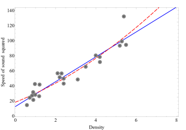
(a) data akm97

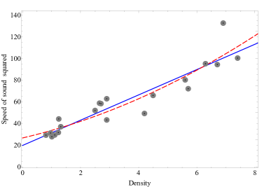
(b) data akm98

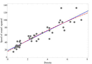
(c) data akm97 $\cup$ akm98

Figure 1: Speed of sound squared (in mm${}^{2}\,$s^-2) versus condensate peak density (in $10^{14}$ cm^-3), for the original data set (a), the corrected data set (b), and their union set (c). The data’s mean values are marked by circles, the curves are their best fits: linear (solid line) and quadratic (dashed curve).

In the formula above, the occurrence of “residual” sound velocity $\bar{c}_{s}\equiv\lim\limits_{n\to\,0}c_{s}=\sqrt{\nu}K$, is surprising; because conventional theory of dilute Bose-Einstein condensates, based on the Gross-Pitaevskii (GP) equation alone gr61 ; pi61 ; gor21 ; psbook , predicts a simpler behaviour $c_{s}\sim n^{1/2}$ (in other words, $\bar{c}_{s}$ would be identically zero in the GP theory). At first look, the difference between these two behaviours is insignificant. However, a nonzero $\bar{c}_{s}$ is not just a curious puzzle; it also raises a profound interpretation problem: if the speed of sound does not vanish when the condensate density decreases down to an infinitesimal value, then what is the physical nature of the matter which remains as $n\to 0$, as compared to a case when no condensate exists ($n\equiv 0$).

An intuitive qualitative answer to this puzzle can be imagined in terms of virtual particles and zero-point fluctuations of the condensate, which is somewhat analogous to the well-known quantum-mechanical phenomenon of non-vanishing energy of a quantum harmonic oscillator in the limit when the number of its modes tends to zero. However, the quantitative description of this phenomenon is more complex, because it requires a model which goes beyond the perturbation theory in general or Gross-Pitaevskii approximation in particular. A working example of such a model in a theory of quantum Bose liquids can be found in Ref. sz19 , but the case of a dilute Bose gas requires some adaption of that framework.

In this paper, we propose a non-perturbative model, which takes into account not only two-body interactions, but also vacuum effects in Bose-Einstein condensates of alkali atoms, and analytically explains the empirical formula (1). In section II we describe a model of a dilute Bose-Einstein condensate, which is expected to resolve the above-mentioned puzzle. In section III we derive the model’s equation of state and hence speed of sound, reproduce the formula (1), and set experimental bounds for the model’s parameters. Conclusions are drawn in section IV.

II The model

We begin by introducing a complex-valued condensate wavefunction $\Psi=\Psi(\textbf{x},t)$, which obeys a normalization condition $\int_{V}|\Psi|^{2}dV=\int_{V}n\,dV={N}$, where $V$ and ${N}$ are, respectively, the total volume and number of particles of the condensate, $n=|\Psi|^{2}$, and $m$ is the mass of the constituent particle (in this case, an alkali atom) psbook .

Aside from this condition, the condensate wavefunction obeys a wave equation, which is defined based on a chosen model. We select the model, which is a special case of the one proposed in Ref. sz19 to describe superfluid helium. Some simplification is possible in the case of the system akm97 ; akm98 , because their cold atom clouds have a much lower density than superfluid helium – which allows us to neglect multiple-body (three or more) interactions. Therefore, in the equations (3) – (6) of Ref. sz19 , one can assume the maximal interaction multiplicity number to be ${\cal N}\equiv 2$. Under these assumptions, we obtain the following wave equation:

$$\left[-i\hbar\,\partial_{t}-\frac{\hbar^{2}}{2m}\vec{\nabla}^{2}+V_{\text{ext}}(\vec{x},\,t)+F(|\Psi|^{2})\right]\Psi=0,$$ (2)

where $V_{\text{ext}}$ is an external/trapping potential, and function $F$ is defined as a sum of two terms

$$F(n)\equiv F_{(\text{ln})}(n)+F_{(2)}(n)=\kappa_{(\text{ln})}\ln{\!\left(n/\bar{n}\right)}+\kappa_{(2)}n,$$ (3)

where we denoted $\kappa_{(\text{ln})}\equiv{\epsilon}C_{(\text{ln})}$, $\kappa_{(2)}\equiv-2{\epsilon}C_{(2)}/\bar{n}$, and ${\epsilon}$ and $\bar{n}$ are scale constants with the dimensions of energy and particle density, respectively, whereas $C$’s are dimensionless coupling coefficients (in notations used in Ref. sz19 ). For the purposes of this paper, in the leading-order approximation the external potential can be neglected, hence we assume the trapless condensate $V_{\text{ext}}\equiv 0$ in what follows, which is a robust approximation for systems of such type kp97 ; z21ijmpb .

Source	Linear best fit					Quadratic best fit
of	$\nu$	$K$	$\kappa_{(\text{ln})}/m$	$\kappa_{(2)}/m$	$\bar{c}_{s}$	$\nu$	$K$	$\kappa_{(\text{ln})}/m$	$\kappa_{(2)}/m$	$\bar{c}_{s}$
data	$(10^{14}\frac{1}{\text{cm}^{3}})$	($10^{-8}\frac{\text{cm}^{5/2}}{\text{s}}$)	($\frac{\text{cm}^{2}}{\text{s}^{2}}$)	($10^{-15}\frac{\text{cm}^{5}}{\text{s}^{2}}$)	($\frac{\text{cm}}{\text{s}}$)	$(10^{14}\frac{1}{\text{cm}^{3}})$	($10^{-8}\frac{\text{cm}^{5/2}}{\text{s}}$)	($\frac{\text{cm}^{2}}{\text{s}^{2}}$)	($10^{-15}\frac{\text{cm}^{5}}{\text{s}^{2}}$)	($\frac{\text{cm}}{\text{s}}$)
akm97	0.77	4.06	0.13	1.65	0.36	1.72	3.27	0.18	1.07	0.43
akm98	1.69	3.42	0.20	1.17	0.44	4.22	2.51	0.27	0.63	0.52
akm97 $\cup$ akm98	1.37	3.63	0.18	1.32	0.42	0.99	3.94	0.15	1.55	0.39

Table 1: Experimental bounds for parameters of the logarithmic-quartic model (2), (3), based on the simplest polynomial best fit functions for $c_{s}^{2}$ data, cf. Fig. 1. The lines refer to, from top to bottom, the original data set akm97 , the corrected data set akm98 , and a union thereof. The quadratic best fit is used only for confirmation of a non-zero value of $\nu$ being a systematic effect, therefore it can be disregarded for the purposes of this paper.

According to these equations, our Bose-Einstein condensate is expected to have a two-part structure (we use the term “part” here to differentiate from physically two-component fluids or mixtures models which use separate wave functions for each component):

First, the part described by the term $F_{(2)}\left(|\Psi|^{2}\right)\propto|\Psi|^{2}$, is responsible for the Gross-Pitaevskii two-body contact interaction discussed above.

The other term $F_{(\text{ln})}\left(|\Psi|^{2}\right)\propto\ln{\left(|\Psi|^{2}/\bar{n}\right)}$ describes the logarithmic fluid part in the wave equation. Nonlinearity of this type often occurs in theories containing quantum Bose liquids and condensates z11appb ; az11 ; z12eb ; z17zna ; z19ijmpb ; sz19 ; z20un1 ; rc21 ; z21ltp ; z21ijmpb . The reason for such universality is that logarithmically nonlinear terms readily emerge in evolution equations for those dynamical systems in which interparticle interaction energies dominate kinetic ones, see Ref. z18zna for more details.

Since the works by Rosen and Bialynicki-Birula and Mycielski ros68 ; bb76 , mathematical properties of (purely) logarithmic nonlinear wave equations have been extensively studied, to mention only very recent literature zsj21 ; itw21 ; ji21 ; liu21 ; liu21fp ; ll21 ; pww21 ; hl21 ; pj21 ; bcs21 ; cf21 ; la21 ; psw21 ; kj22 ; sav22 ; yzq22 ; aea21 ; zsw22 ; pjh22 ; vgm22 ; cs22nu ; pen22 ; but combined logarithmic-polynomial nonlinearities, like the one occurring in our model, still await thorough study.

III Equation of state and speed of sound

Using the Madelung representation of a wavefunction, one can rewrite any nonlinear wave equation of type (2) in hydrodynamic form. One can derive the general expressions for an equation of state and speed of sound $c_{s}$, which become quite simple if we retain only the leading-order terms with respect to the Planck constant z19mat . When evaluated on a function (3), those formulae yield, respectively, an equation of state and speed of sound for our model:

$$P \approx \int nF^{\prime}(n)dn=\kappa_{(\text{ln})}n+\kappa_{(2)}n^{2}/2,$$ (4)

$$c_{s}^{2} \equiv \frac{1}{m}\frac{\partial P}{\partial n}\approx\frac{1}{m}\left(\kappa_{(\text{ln})}+\kappa_{(2)}n\right),$$ (5)

where the approximation symbol means that we kept only the leading-order terms with respect to the Planck constant. In the derived equation of state, one can notice the Bogoliubov term, which is quadratic in density and induced by the Gross-Pitaevskii part of our model, cf. Eq. (3). This is an expected effect of the GP model psbook . However, one can also notice the linear term, which is well-known from ideal gas models. It is interesting that here it comes from the logarithmic part of our model.

Furthermore, formula (5) can be written as

$$c_{s} \approx \sqrt{\frac{\kappa_{(2)}}{m}}\left(n+\frac{\kappa_{(\text{ln})}}{\kappa_{(2)}}\right)^{1/2},$$ (6)

which reproduces the empirical formula (1), once we make the following associations:

$$\nu\Leftrightarrow\kappa_{(\text{ln})}/\kappa_{(2)},\ \ K^{2}\Leftrightarrow\kappa_{(2)}/m,$$ (7)

thus one can see that it is the logarithmic nonlinearity which induces the constant term $\nu$ in an expression for the speed of sound squared. Inverting these formulae, we obtain the following relations between parameters of our model and experimentally measured values:

$$\kappa_{(\text{ln})}=m\,\nu K^{2},\ \ \kappa_{(2)}=mK^{2},$$ (8)

which can be used to place empirical bounds on the model’s parameters.

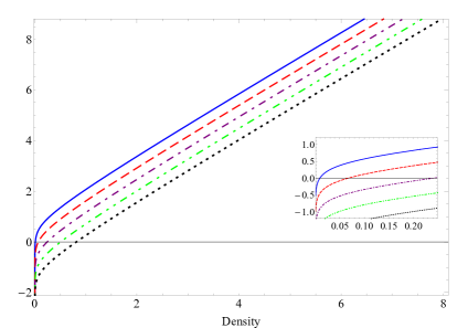
Figure 2: Profile of $F(n)/m$ (in cm${}^{2}\,$s^-2), versus condensate density $n$ (in $10^{14}$ cm^-3), for different scales of $\bar{n}$ (in $10^{14}$ cm^-3): 0.01 (solid), 0.1 (dashed), 1 (dash-dotted), 10 (dash-double-dotted) and 100 (dotted). Values of $\kappa$’s are taken from the linear best bit of data akm98 , see Table 1.

In Table 1, we show these constraints, based on linear and quadratic best fit functions of $c_{s}^{2}$ data, as described in Fig. 1. These are placed on the parameters $\kappa_{(\text{ln})}$ and $\kappa_{(2)}$ of the model (2), (3), but not on the parameter $\bar{n}$ which determines the characteristic density scale of logarithmic nonlinearity. This parameter is thus assumed to be a free parameter of our model for now, but one can think of various ways of how to determine its value in future experiments.

For example, one can think of an experiment which is sensitive to the transition of function $F(n)$ between its positive and negative values’ regimes (the existence of such a transition is theoretically predicted, as it can be seen directly from Fig. 2). If such a transition occurs, the critical density value $n_{c}$ exists at which $F(n)$ momentarily turns to zero before flipping its sign. Then the density scale parameter of the logarithmic nonlinearity would be related to this value as

$$\bar{n}=n_{c}\exp{\left(\kappa_{(2)}n_{c}/\kappa_{(\text{ln})}\right)}=n_{c}\exp{\left(n_{c}/\nu\right)},$$ (9)

according to Eqs. (3) and (8).

IV Conclusion

To summarize, we formulated a two-part Bose-Einstein condensate model, involving both logarithmic and Gross-Pitaevskii nonlinearities, which is a truncated version of the model previously used by us for superfluid helium. In this model, the Gross-Pitaevskii two-body interaction term is suggested by the perturbation theory of dilute Bose-Einstein condensates; whereas the logarithmic term is essentially non-perturbative, and takes into account quantum vacuum effects. Our model has excellent agreement with the sound propagation data in the condensate of cold sodium atoms by Andrews et al., where the logarithmic term induces a shift constant in the asymptotic behaviour of sound velocity at infinitesimal values of density, while the Gross-Pitaevskii term defines a shape of the curve itself. The data also allowed us to place constraints for two of the model’s parameters, which describe the strength of the logarithmic and Gross-Pitaevskii terms. Furthermore, we suggested an experiment constraining the value of the third parameter (the density scale of the logarithmic component of the model); based on the conjectured attraction–repulsion transition of the resulting many-body interaction in the condensate.

- (1) M. R. Andrews, D. M. Kurn, H.-J. Miesner, D. S. Durfee, C. G. Townsend, S. Inouye and W. Ketterle, Phys. Rev. Lett. 79, 553 (1997).
- (2) M. R. Andrews, D. M. Stamper-Kurn, H.-J. Miesner, D. S. Durfee, C. G. Townsend, S. Inouye and W. Ketterle, Phys. Rev. Lett. 80, 2967 (1998).
- (3) K. G. Zloshchastiev, J. Phys.: Conf. Ser. 2103, 012200 (2021).
- (4) E. P. Gross, Nuov. Cim. 20, 454 (1961).
- (5) L. P. Pitaevskii, Sov. Phys. JETP 13, 451 (1961).
- (6) R. A. Van Gorder, Proc. R. Soc. A 477, 20210443 (2021).
- (7) C. J. Pethick and H. Smith, Bose-Einstein Condensation in Dilute Gases (Cambridge University Press, New York, 2008).
- (8) T. C. Scott and K. G. Zloshchastiev, Low Temp. Phys. 45, 1231 (2019).
- (9) G. M. Kavoulakis and C. J. Pethick, Phys. Rev. A 58, 1563 (1997).
- (10) K. G. Zloshchastiev, Int. J. Mod. Phys. B 35, 2150229 (2021).
- (11) K. G. Zloshchastiev, Acta Phys. Polon. 42, 261 (2011).
- (12) A. V. Avdeenkov and K. G. Zloshchastiev, J. Phys. B: At. Mol. Opt. Phys. 44, 195303 (2011).
- (13) K. G. Zloshchastiev, Eur. Phys. J. B 85, 273 (2012).
- (14) K. G. Zloshchastiev, Z. Naturforsch. A 72, 677 (2017).
- (15) K. G. Zloshchastiev, Int. J. Mod. Phys. B 33, 1950184 (2019).
- (16) K. G. Zloshchastiev, Universe 6, 180 (2020).
- (17) O. A. Rodríguez-López and E. Castellanos, J. Low Temp. Phys. 204, 111 (2021).
- (18) K. G. Zloshchastiev, Low Temp. Phys. 47, 89 (2021).
- (19) K. G. Zloshchastiev, Z. Naturforsch. A 73, 619 (2018).
- (20) G. Rosen, J. Math. Phys. 9, 996 (1968).
- (21) I. Bialynicki-Birula and J. Mycielski, Ann. Phys. (N. Y.) 100, 62 (1976).
- (22) F. Zeng, P. Shi and M. Jiang, AIMS Math. 6, 2559 (2021).
- (23) N. Ikoma, K. Tanaka, Z.-Q. Wang and C. Zhang, Nonlinearity 34, 1900 (2021).
- (24) C. Ji, Z. Angew. Math. Phys. 72, 70 (2021).
- (25) C.-S. Liu, Commun. Theor. Phys. 73, 045007 (2021).
- (26) C.-S. Liu, Nonlinear Dyn. 106, 899 (2021).
- (27) C. N. Le and X. T. Le, Math. Bohem. 147, 33 (2022).
- (28) B. Peng, Y. Wang and G. Wei, J. Math. Anal. Appl. 498, 124963 (2021).
- (29) S. He and X. Liu, Partial Differ. Equ. Appl. 2, 70 (2021).
- (30) X. Peng and G. Jia, Z. Angew. Math. Phys. 72, 198 (2021).
- (31) W. Bao, R. Carles, C. Su and Q. Tang, Math. Models Methods Appl. Sci. 32, 101 (2022).
- (32) R. Carles and G. Ferriere, Nonlinearity 34, 8283 (2021).
- (33) F. C. E. Lima and C. A. S. Almeida, Eur. Phys. J. C 81, 1044 (2021).
- (34) L. Peng, H. Suo, D. Wu, H. Feng and C. Lei, Electron. J. Qual. Theory Differ. Equ. 90, 1 (2021).
- (35) Y. Kai, J. Ji and Z. Yin, Nonlinear Dyn. 107, 2745 (2022).
- (36) S. E. Savotchenko, Pramana - J. Phys. 96, 47 (2022).
- (37) J. Yan, H. Zhang, X. Qian, X. Chen and S. Song, Appl. Numer. Math. 176, 19 (2022).
- (38) A. Abolarinwa, J. O. Ehigie and A. H. Alkhaldi, J. Geom. Phys. 170, 104382 (2021).
- (39) Z. Zhou, J. Song, W. Weng and Z. Yan, Appl. Math. Lett. 132, 108131 (2022).
- (40) X. Peng, G. Jia and C. Huang, Math. Meth. Appl. Sci. Online, DOI: 10.1002/mma.8260 (2022).
- (41) R. van Geleuken and A. V. Martin, Phys. Rev. A 105, 1032210 (2021).
- (42) R. Carles and C. Su, Commun. Partial Differ. Equ. Online, DOI: 10.1080/03605302.2022.2050257 (2022).
- (43) X. Peng, J. Math. Anal. Appl. 513, 126249 (2022).
- (44) K. G. Zloshchastiev, J. Theor. Appl. Mech. 57, 843 (2019).