DGRec: Graph Neural Network for Recommendation with Diversified Embedding Generation

Abstract.

Graph Neural Network (GNN) based recommender systems have been attracting more and more attention in recent years due to their excellent performance in accuracy. Representing user-item interactions as a bipartite graph, a GNN model generates user and item representations by aggregating embeddings of their neighbors. However, such an aggregation procedure often accumulates information purely based on the graph structure, overlooking the redundancy of the aggregated neighbors and resulting in poor diversity of the recommended list. In this paper, we propose diversifying GNN-based recommender systems by directly improving the embedding generation procedure. Particularly, we utilize the following three modules: submodular neighbor selection to find a subset of diverse neighbors to aggregate for each GNN node, layer attention to assign attention weights for each layer, and loss reweighting to focus on the learning of items belonging to long-tail categories. Blending the three modules into GNN, we present DGRec (Diversified GNN-based Recommender System) for diversified recommendation. Experiments on real-world datasets demonstrate that the proposed method can achieve the best diversity while keeping the accuracy comparable to state-of-the-art GNN-based recommender systems. We open source DGRec at https://github.com/YangLiangwei/DGRec.

1. Introduction

We live in an era of information overflow (Mayer-Schönberger and Cukier, 2013), with data created every moment too large to digest in time. Recommender systems (Wang et al., 2021, 2014, 2012; Sun et al., 2012) target mitigating the problem by providing people with the most relevant information in the massive data. Recommender systems play an essential role in our daily life, such as the news feed (Wu et al., 2019), music suggestions (Chen et al., 2018a), online advertising (Gao et al., 2021), and shopping recommendations (Gu et al., 2020). To maximize the utility of recommendation systems, accuracy is often the only criterion measuring how likely the users would interact with given items. Companies and researchers have been building sophisticated methods (Wang et al., 2022; Yang et al., 2021) to optimize accuracy during all steps in recommender systems.

However, a well-designed recommender system should be evaluated from multiple perspectives, e.g. diversity (Zheng et al., 2021). Accuracy can only reflect correctness, and pure accuracy-targeted methods may lead to the echo chamber/filter bubble (Ge et al., 2020) effects, trapping users in a small subset of familiar items without exploring the vast majority of others. To break the filter bubble, diversification in recommender systems is receiving increasing attention. Through an online A/B test, research (Huang et al., 2021) shows that the number of users’ engagements and the average time spent greatly benefit from diversifying the recommender systems. Diversified recommendation targets increase the dissimilarity among recommended items to capture users’ varied interests. Nevertheless, optimizing diversity alone often leads to decreases in accuracy. Accuracy and diversity dilemma (Zhou et al., 2010) reflects such a trade-off. Therefore, diversified recommender systems aim to increase diversity with minimal costs on accuracy (Zheng et al., 2021; Ashkan et al., 2015; Chen et al., 2018b).

Graph-based recommender systems (Wang et al., 2021) have attracted more and more research attention. Graph-based methods have several advantages. Representing users’ historical interactions as a user-item bipartite graph can give us easy access to high-order connectivities. Graph neural network (Scarselli et al., 2008) is a family of powerful learning methods for graph-structured data (He et al., 2021; Liang et al., 2018). The common practice of graph-based recommender systems is designing suitable graph neural networks to aggregate information from the neighborhood of every node to generate the node embedding. This procedure also provides opportunities for diversified recommendation (Zheng et al., 2021). Firstly, the user/item embedding is easily affected by its neighbors, and we can manipulate the choice of neighbors to obtain a more diversified embedding representation. Secondly, the unique high-order neighbors of each user/item node can provide us with personalized distant interests for diversification, which can be naturally captured by stacking multiple GNN layers.

Achieving diversified recommendations using GNNs comes with the following challenges. Firstly, how to effectively manipulate the neighborhood to increase diversity is still an open question. The popular ones will submerge the long-tail items if we have a direct aggregation on all neighbors. Secondly, the over-smoothing problem (Liu et al., 2020) occurs when directly stacking multiple GNN layers. Over-smoothing would lead to similar representations among nodes in the graph, dramatically decreasing the accuracy performance. Thirdly, as seen in Figure 1, the item occurrence in data and the number of items within each category both follow the power-law distribution. Training under such distribution would focus on the popular items/categories, which only constitute a small part of the items/categories. Meanwhile, the long-tail items/categories are un-perceptible during the training stage. Researches in graph-based diversified recommendation is very limited. Early endeavors (Zhou et al., 2010) assign different probabilities on edges to boost the information flow of long-tail items. DGCN (Zheng et al., 2021) is the first work to diversify over graph neural networks. It fails to consider the high-order connectivities and the long tail categories.

In this paper, we propose DGRec to cope with the previously mentioned challenges. We design the following three modules. 1. Submodular neighbor selection firstly integrates submodular optimization into GNN. It finds a diversified subset of neighbors by optimizing a submodular function. Information aggregated from the diversified subset can help us uncover the long-tail items and reflect them in the aggregated representation. 2. Layer attention aims to handle the over-smoothing problem. It stabilizes the training on deep GNN layers and enables DGRec to take advantage of high-order connectivities for diversification. 3. Loss reweighting reduces the weight on popular items/categories. It assists the model in focusing more on the long-tail items/categories. Our contributions are summarized as follows:

• We design three modules for the diversified recommendation and propose DGRec that achieves the best trade-off between accuracy and diversity.

• The three modules can be easily applied to graph neural network based methods to increase recommendation diversity with a small cost on accuracy.

• We conduct extensive experiments on real-world datasets to show the effectiveness of DGRec and the influences of different modules.

The remaining paper is organized as follows. Section 2 gives the required preliminaries. Section 3 illustrates DGRec in detail and the three proposed modules for diversification. Section 4 conducts extensive experiments to evaluate the effectiveness of DGRec, and discusses the influence of different modules. Section 5 represents the most related works for reference, and we conclude DGRec and discuss future research directions in Section 6.

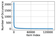
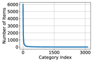
Figure 1. Long tail distribution in Recommender System on TaoBao dataset (Zheng et al., 2021).

2. Preliminaries

This section introduces some work preliminaries, including task formulation, graph neural network, and accuracy-diversity dilemma.

2.1. Problem Statement

For diversified recommendation task, we have a set of users $\mathcal{U}=\{u_{1},u_{2},...,u_{\left|\mathcal{U}\right|}\}$, a set of items $\mathcal{I}=\{i_{1},i_{2},...,i_{\left|\mathcal{I}\right|}\}$, and a mapping function $C(\cdot)$ that maps each item to its category. The observed user-item interactions can be represented as an interaction matrix $\textbf{R}\in\mathbb{R^{\left|\mathcal{U}\right|\times\left|\mathcal{I}\right|}}$, where $R_{u,i}=1$ if user $u$ has interacted with item $i$, or $R_{u,i}=0$ otherwise. For a graph based recommender model, the historical interactions are represented by a user-item bipartite graph $\mathcal{G}=(\mathcal{V},\mathcal{E})$, where $\mathcal{V}=\mathcal{U}\cup\mathcal{I}$ and there is an edge $e_{u,i}\in\mathcal{E}$ between $u$ and $i$ if $R_{u,i}=1$.

Learning from the user-item bipartite graph $\mathcal{G}$, a recommender system aims to recommend top $k$ interested items $\{i_{1},i_{2},...,i_{k}\}$ for each user $u$. The diversified recommendation task requires the top $k$ recommended items to be dissimilar to each other. The dissimilarity (or diversity) of a recommended list is usually measured by the coverage of recommended categories $|\cup_{i\in\{i_{1},\ldots,i_{k}\}}C(i)|$ (Puthiya Parambath et al., 2016; Zheng et al., 2021).

2.2. Graph Neural Network

A Graph Neural Network is a deep learning model that operates on graph structures, and it has achieved great success in the application of many real-world tasks with graph-structured data, including social networks (Yang et al., 2022b; Liu et al., 2022b), email networks (Liu et al., 2022a) and user-item interaction graphs in recommender systems (Yang et al., 2022a). A GNN model learns the representations of node embeddings by aggregating information from their neighbors, so that connected nodes in the graph structure tend to have similar embeddings. The operation of a general GNN computation can be expressed as follows:

(1) $$\mathbf{e}_{u}^{(l+1)}=\mathbf{e}_{u}^{(l)}\oplus\text{AGG}^{(l+1)}(\{\mathbf{e}_{i}^{(l)}\mid i\in\mathcal{N}_{u}\}),$$

where $\mathbf{e}_{u}^{(l)}$ indicates node $u$’s embedding on the $l$-th layer, $\mathcal{N}_{u}$ is the neighbor set of node $u$, $\mbox{AGG}^{(l)}(\cdot)$ is a function that aggregates neighbors’ embeddings into a single vector for layer $l$, and $\oplus$ combines $u$’s embedding with its neighbor’s information. AGG$(\cdot)$ and $\oplus$ can be simple or complicated functions.

2.3. Submodular Function

A submodular function is a set function defined on a ground set $V$ of elements: $f:2^{V}\rightarrow\mathbb{R}$. The key defining property of submodular functions is the diminishing-returns property, i.e.,

(2) $$f(v|A)\geq f(v|B)\quad\forall A\subset B\subset V,\ v\in V\text{ and }v\notin B.$$

Here we use a shorthand notation $f(v|A):=f(\{v\}\cup A)-f(A)$ to represent the gain of an element $v$ conditioned on the set $A$. The diminishing-returns property naturally describes the diversity of a set of elements, and submodular functions have been applied to various diversity-related machine learning tasks with great success in practice, such as text summarization, sensor placement, and training data selection (Zheng et al., 2014; Hoi et al., 2006). Submodular functions are also applied as a re-ranking method to diversify recommendations, which is orthogonal to the relevance prediction model. Submodular functions also exhibit nice theoretical properties to be solved with strong approximation guarantees using efficient algorithms (Nemhauser et al., 1978).

3. Method

In this section, we first present the backbone GNN-based recommender system of DGRec, and then illustrate the three modules to obtain diversified recommendations during the embedding generation procedures. The framework of DGRec is shown in Figure 2. More specifically, it consists of the following components: Submodular neighbor selection, Layer attention and Loss reweighting.

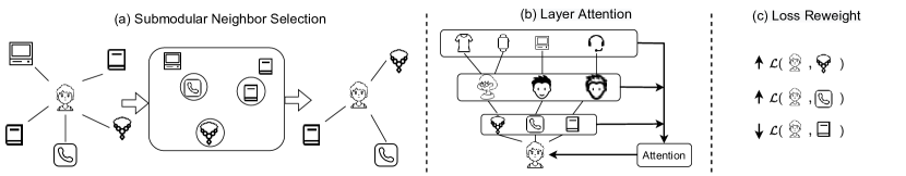
Figure 2. The framework of DGRec. (a) Submodular neighbor selection module (Section 3.2) finds a diversified subset of neighbors on the embedding space for aggregation. (b) Layer attention module (Section 3.3) alleviates the over-smoothing problem from high-order connections. (c) Loss reweighting module (Section 3.4) adjusts weight for each sample to focus on the training of long-tail categories.

3.1. Overall Training Framework

Based on the user-item bipartite graph $\mathcal{G}$, a GNN-based recommender system generates user/item embeddings by graph neural networks to predict user’s preference.

3.1.1. Embedding Layer

Similar to the learning representation of words and phrases, the embedding technique is also widely used in recommender systems (He et al., 2020; Rendle et al., 2012): an embedding layer is a look-up table that maps the user/item ID to a dense vector:

(3) $$\textbf{E}^{(0)}=\left(\textbf{e}_{1}^{(0)},\textbf{e}_{2}^{(0)},\ldots,\textbf{e}_{|\mathcal{U}|+|\mathcal{I}|}^{(0)}\right),\\$$

where $\mathbf{e}^{(0)}\in\mathbb{R}^{d}$ is the $d$-dimensional dense vector for user/item. An embedding indexed from the embedding table is then fed into a GNN for information aggregation. Thus it is noted as the ”zero”-th layer output $\mathbf{e}_{i}^{(0)}$.

3.1.2. Light Graph Convolution

We utilize the light graph convolution (He et al., 2020) (LGC) as the backbone GNN layer. It abandons the feature transformation and nonlinear activation, and directly aggregates neighbors’ embeddings, and is defined as:

(4) $$\mathbf{e}_{u}^{(l+1)}=\sum_{i\in\mathcal{N}_{u}}\frac{1}{\sqrt{|\mathcal{N}_{u}|}\sqrt{|\mathcal{N}_{i}|}}\mathbf{e}_{i}^{(l)},$$

$$\mathbf{e}_{i}^{(l+1)}=\sum_{u\in\mathcal{N}_{i}}\frac{1}{\sqrt{|\mathcal{N}_{i}|}\sqrt{|\mathcal{N}_{u}|}}\mathbf{e}_{u}^{(l)},$$

where $\mathbf{e}_{u}^{(l)}$ and $\mathbf{e}_{i}^{(l)}$ are user $u$’s and item $i$’s embedding at the $l$-th layer, respectively. $\frac{1}{\sqrt{|\mathcal{N}_{u}|}\sqrt{|\mathcal{N}_{i}|}}$ is the normalization term following GCN (Kipf and Welling, 2017). $\mathcal{N}_{u}$ is $u$’s neighborhood that selected by submodular function as illustrated in Section 3.2. Each LGC layer would generate one embedding vector for each user/item node. Embedding generated from different layers are from the different receptive field. The final user/item representation is obtained by layer attention illustrated in Section 3.3:

(5) $$\mathbf{e}_{u}=\text{Layer\_Attention}\left(\mathbf{e}_{u}^{(0)},\mathbf{e}_{u}^{(1)},\ldots,\mathbf{e}_{u}^{\text{(layer num)}}\right),$$

$$\mathbf{e}_{i}=\text{Layer\_Attention}\left(\mathbf{e}_{i}^{(0)},\mathbf{e}_{i}^{(1)},\ldots,\mathbf{e}_{i}^{\text{(layer num)}}\right).$$

3.1.3. Model Optimization

After we obtain $\mathbf{e}_{u}$ and $\mathbf{e}_{i}$, the score of $u$ and $i$ pair is calculated by dot product of the two vectors. For each positive pair $(u,i)$, a negative item $j$ is randomly sampled to compute the Bayesian personalized ranking (BPR) (Rendle et al., 2012) loss. To increase recommendation diversity, we propose to reweight the loss to focus more on the long-tail categories:

(6) $$\mathcal{L}=\sum_{(u,i)\in\mathcal{E}}w_{C(i)}\mathcal{L}_{bpr}(u,i,j)+\lambda{\left\|\Theta\right\|}_{2}^{2},$$

where $w_{C(i)}$ is the weight for each sample based on its category, which is illustrated in Section 3.4. $\lambda$ is the regularization factor. $j$ is a randomly sampled negative item.

3.2. Submodular Neighbor Selection

In GNN-based recommender systems, user/item embedding is obtained by aggregating information from all neighbors. Popular items would overwhelm the long-tail items. In Figure 2(a), the user’s embedding would be much more similar to books if we aggregate all the neighbors. At the same time, the necklace information is overwhelmed in the user’s representation. The submodular neighbor selection module aims to select a set of diverse neighbors for aggregation. In our setting of GNN neighbor selection, the ground set for a user node $u$ consists of all of its neighbors $\mathcal{N}_{u}$. Facility location function (Cornuejols et al., 1977) is a widely used submodular function that evaluates the diversity of a subset of items by first identifying the most similar item in the selected subset $\mathcal{S}_{u}$ to every item $i$ in the ground set ($\max_{i^{\prime}\in\mathcal{S}_{u}}\text{sim}(i,i^{\prime})$ $\forall i\in\mathcal{N}_{u}\backslash\mathcal{S}_{u}$) and then summing over the similarity values. Intuitively, a subset with a high function value indicates that for every item in the ground set, there exists a similar item in the selected subset, or in other words, the selected subset is very diverse and representative of the ground set. The facility location function is formally defined as follows:

(7) $$f(\mathcal{S}_{u})=\sum_{i\in\mathcal{N}_{u}\backslash\mathcal{S}_{u}}\max_{i^{\prime}\in\mathcal{S}_{u}}\text{sim}(i,i^{\prime}),$$

where $\mathcal{S}_{u}$ is the selected neighbor subset of user $u$, and $\text{sim}(i,i^{\prime})$ is the similarity of $i$ and $i^{\prime}$, which is measured by Gaussian kernel parameterized by a kernel width $\sigma^{2}$:

(8) $$\text{sim}(i,i^{\prime})=\text{exp}\left(-\frac{||\mathbf{e}_{i}-\mathbf{e}_{i^{\prime}}||^{2}}{\sigma^{2}}\right).$$

$\mathcal{S}_{u}$ is constrained to having no greater than $k$ items for some constant $k$, i.e., $|\mathcal{S}_{u}|\leq k$. Maximizing the submodular function (7) under cardinality constraint is NP-hard, but it can be approximately solved with $1-e^{-1}$ bound by the greedy algorithm (Nemhauser et al., 1978). The greedy algorithm starts with an empty set $\mathcal{S}_{u}:=\emptyset$, and adds one item $i\in\mathcal{I}\backslash\mathcal{S}_{u}$ with the largest marginal gain to $\mathcal{S}_{u}$ every step:

(9) $$\mathcal{S}_{u}\leftarrow\mathcal{S}_{u}\cup i^{*},$$

$$i^{*}=\operatorname*{arg\,max}_{i\in\mathcal{N}_{u}\backslash\mathcal{S}_{u}}\ [f(\mathcal{S}_{u}\cup i)-f(\mathcal{S}_{u})].$$

After $k$ steps of greedy neighbor selection, we can obtain the diversified neighborhood subset of each user. The subset is then used for aggregation. We also note that our framework works for any choice of a submodular function. We choose the facility location function as it is generally applicable to numerical features (with certain similarity metric). We also discuss other choices of submodular functions in the empirical studies.

3.3. Layer Attention

Different GNN layers generate embeddings based on information from different subsets of nodes: the $l$-th layer would aggregate from the $l$-th hop neighbors. We can reach a diversified embedding by aggregating from the high-order neighbors. However, the direct stack of several GNN layers would cause the over-smoothing problem (Liu et al., 2020). As shown in Figure 2(b), layer attention is designed in DGRec to increase diversity by high-order neighbors and mitigate the over-smoothing problem at the same time.

For each user/item, we have $L$ embeddings generated by $L$ GNN layers. Layer attention aims to get the final representation by learning a Readout function on $[\mathbf{e}^{(0)},\mathbf{e}^{(1)},\ldots,\mathbf{e}^{(L)}]$ by attention (Liu et al., 2021):

(10) $$\mathbf{e}=\text{Readout}([\mathbf{e}^{(0)},\mathbf{e}^{(1)},\ldots,\mathbf{e}^{(L)}])=\sum_{l=0}^{L}a^{(l)}\mathbf{e}^{(l)},$$

where $a^{(l)}$ is the attention weight for $l$-th layer. It is calculated as:

(11) $$a^{(l)}=\frac{\text{exp}(\langle\mathbf{W}_{\text{Att}},\mathbf{e}^{(l)}\rangle)}{\sum_{l^{\prime}=0}^{\text{L}}\text{exp}(\langle\mathbf{W}_{\text{Att}},\mathbf{e}^{(l^{\prime})}\rangle)}.$$

Here $\mathbf{W}_{\text{Att}}\in\mathbb{R}^{d}$ is the parameter for attention computation. The attention mechanism can learn different weights for GNN layers to optimize the loss function. It can effectively alleviate the over-smoothing problem (Liu et al., 2021).

3.4. Loss Reweighting

As shown in Figure 1, the number of items within each category is highly imbalanced and follows the power-law distribution. A small number of categories contains the most items while leaving the large majority of categories with only a limited number of items. Training the model by directly optimizing the mean loss over all samples would leave the training of long-tail categories imperceptible. In DGRec, we propose to reweight the sample loss during training based on its category. As shown in Figure 2(c), DGRec would decrease the weight relatively if the item belongs to popular categories, and increase the weight relatively if it belongs to long-tail categories.

In practice, we borrow the idea of class-balanced loss (Cui et al., 2019) to reweight the sample $(u,i)$ based on the category effective number of items. The weights $w_{C(i)}$ in Equation 6 are calculated by:

(12) $$w_{C(i)}=\frac{1-\beta}{1-\beta^{|C(i)|}},$$

where $\beta$ is the hyper-parameter that decides the weight. A larger $\beta$ would further decrease the weight of popular categories.

4. Experiment

In this section, We conduct extensive experiments on two real-world datasets to answer the following research questions (RQs):

• RQ1: Does DGRec outperform existing methods in the diversified recommendation?

• RQ2: How do the hyper-parameters influence DGRec, and how can we trade off accuracy and diversity in DGRec?

• RQ3: Are the three components in DGRec necessary to boost diversification?

• RQ4: What is the influence of different submodular functions?

4.1. Experimental Setup

4.1.1. Datasets

To evaluate the effectiveness of DGRec, we conduct experiments on two real-world datasets with category information. The statistics of the two datasets are shown in Table 1.

• TaoBao (Zheng et al., 2021): This dataset contains users’ behavior on TaoBao platform, which was provided by Alimama. This dataset contains users’ multiple kinds of behaviors, including clicking, purchasing, adding items to carts, and item favoring. All those behaviors are treated as positive samples. To ensure the quality of the dataset, the 10-core setting is adopted, i.e., only users/items with at least $10$ interactions are retained.

• Beauty (Liang et al., 2021): This dataset contains product review information and metadata from Amazon. Following the setting in (Liang et al., 2021), the 5-core version is adopted to ensure data quality.

For both datasets, we randomly split out $60\%$ for training, $20\%$ for validation, and $20\%$ for testing. Validation sets are used for hyper-parameter tuning and early stopping. We report results on the test set as the final results.

Table 1. Statistics of the Datasets

Dataset	TaoBao	Beauty
Users	82,633	8,159
Items	136,710	5,862
Interactions	4,230,631	98,566
Categories	3,108	41
Average Category Size	43.986	139.595

4.1.2. Baselines

To empirically evaluate and study DGRec, we compare our model with representative recommender system baselines. Note that DGRec is compatible with the re-ranking-based methods such as DPP (Chen et al., 2018b), MMR (Carbonell and Goldstein, 1998), DUM (Ashkan et al., 2015) and Diversified PMF (Sha et al., 2016). Thus we do not compare those methods in the experiments. Selected baselines are shown as follows:

• Popularity: It is a non-personalized recommendation method that only recommends popular items to users.

• MF-BPR (Rendle et al., 2012): It factorizes the interaction matrix into user and item latent factors.

• GCN (Kipf and Welling, 2017): It is one of the most widely used graph neural networks.

• LightGCN (He et al., 2020): It is the state-of-the-art recommender system. LightGCN is a GCN-based model but removes the transformation matrix, non-linear activation, and self-loop.

• DGCN (Zheng et al., 2021): It is the current state-of-the-art diversified recommender system based on GNN.

4.1.3. Evaluation Metrics

Following previous works (Zheng et al., 2021; Chen et al., 2018b; Cheng et al., 2017), we use two different kinds of metrics to evaluate the accuracy and diversity respectively. We aim to get a diversified item set during the retrieval stage, so Recall and Hit Ratio (HR) are used to measure the accuracy. Coverage is used to measure diversity, which counts the number of covered categories of recommended items. To save space, we only report Top-100 and Top-300 retrieval results. We can reach the same conclusion for other top-N retrievals.

4.1.4. Parameter Setting

In experiments, we tune all the baselines using the validation set and report the results on the test set. Adam (Kingma and Ba, 2014) is used as the optimizer. Following the setting of DGCN, we fix the embedding size to be $32$ and randomly sample $4$ negative items for each positive user-item pair for a fair comparison. Other hyper-parameters are tuned by grid search. Early stopping is utilized to alleviate the over-fitting problem. We stop training if the performance on validation set does not improve in $10$ epochs.

4.2. Performance Evaluation (RQ1)

Table 2. Overall comparison on TaoBao dataset, the best and second-best results are in bold and underlined, respectively.

Method	TaoBao
	Recall@100	Recall@300	HR@100	HR@300	Coverage@100	Coverage@300
Popularity	0.0186	0.0357	0.1496	0.2562	38.2449	75.9837
MF-BPR (Rendle et al., 2012)	0.0487	0.0971	0.3103	0.4889	34.0812	71.8802
GCN (Kipf and Welling, 2017)	0.0446	0.0923	0.2840	0.4634	37.2577	79.2985
LightGCN (He et al., 2020)	0.0528	0.1063	0.3261	0.5097	32.7069	69.3502
DGCN (Zheng et al., 2021)	0.0394	0.0831	0.2634	0.4369	38.1183	84.4989
DGRec	0.0472	0.0951	0.3026	0.4817	39.0597	89.1684

Table 3. Overall comparison on Beauty dataset, the best and second-best results are in bold and underlined, respectively.

Method	Beauty
	Recall@100	Recall@300	HR@100	HR@300	Coverage@100	Coverage@300
Popularity	0.1012	0.2096	0.1833	0.3124	16.0213	27.9336
MF-BPR (Rendle et al., 2012)	0.2310	0.3863	0.3404	0.4966	15.8728	25.6659
GCN (Kipf and Welling, 2017)	0.2388	0.3897	0.3423	0.3897	16.5311	25.5634
LightGCN (He et al., 2020)	0.2517	0.4205	0.3688	0.5318	15.0203	23.9421
DGCN (Zheng et al., 2021)	0.2395	0.3790	0.3418	0.4792	18.2876	26.9694
DGRec	0.2399	0.3915	0.3420	0.5021	19.0557	27.5704

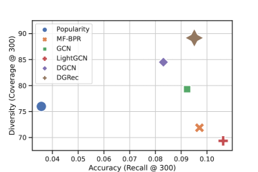
Figure 3. Accuracy-Diversity trade-off comparison on TaoBao dataset. The upper-right model is enlarged.

We report the experiment results in Table 2 (TaoBao dataset) and Table 3 (Beauty dataset). We have the following observations:

• DGRec generally achieves the best on Coverage@100 and Coverage@300 except being second to Popularity in terms of Coverage@300 on the Beauty dataset. Considering Coverage@300 on the Beauty dataset, DGRec is just slightly lower than Popularity. It shows that DGRec can achieve the most diversified recommendation results.

• Though LightGCN always achieves the best Recall and Hit Ratio, its Coverage is always the lowest. It shows that LightGCN can not achieve an accuracy-diversity balance.

• While achieving the best Coverage, DGRec has similar results with the second best on Recall and Hit Ratio. It shows DGRec increases the diversity with a small cost on the accuracy, which well balances the accuracy-diversity trade-off.

• DGRec surpasses DGCN on all metrics. It shows DGRec surpasses the SoTA model, and the design of DGRec is superior in both accuracy and diversity.

To make a clearer comparison of all methods, we illustrate the accuracy-diversity trade-off in Figure 3. Accuracy and diversity are measured by Recall@300 and Coverage@300, respectively. We can clearly observe that DGRec stands in the most upper-right position, which shows DGRec achieves the best trade-off. Compared with DGRec, all other models with similar accuracy (GCN, MF-BPR) have an obvious drop in diversity. Compared with LightGCN, DGRec greatly increases diversity with a small sacrifice on accuracy.

4.3. Parameter Sensitivity (RQ2)

In this section, we study the influence of different hyper-parameters on DGRec, and how to trade-off between accuracy/diversity.

4.3.1. Layer Number.

The layer number is an influential hyper-parameter in the GNN-based recommender system, which indicates the number of GNN layers stacked to generate the user/item embedding. We compare our proposed layer attention with the mean aggregation (He et al., 2020) on both accuracy and diversity. Experimental results are shown in Figure 4. With the mean aggregation, we can see Recall@300 drops quickly with the increase of layers. It reflects the well-known over-smoothing problem (Liu et al., 2020) in GNN. The increase in Coverage@300 verifies our hypothesis that we can obtain a diverse embedding representation by adding more information from higher-order connections. However, mean aggregation does not make an effective trade-off between accuracy and diversity. The sharp drop on Recall@300 makes the increased diversity meaningless. With the proposed layer attention, DGRec does not suffer from the over-smoothing problem and achieves gradually increased Recall@300 with the increase of layers. It shows layer attention can effectively learn different attention weights for each layer to fit the data. At the same time, DGRec generally achieves a high Coverage@300. It shows the layer attention module can retain a good performance on diversity with a different number of layers. When mean aggregation and layer attention achieve similar Recall@300 (2 layers), Coverage@300 of layer attention is much larger than mean aggregation. The case is similar if we compare Recall@300 when they achieve similar Coverage@300. It shows layer attention used in DGRec can achieve a much better accuracy diversity trade-off than mean aggregation.

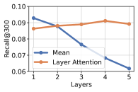
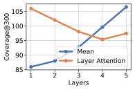
Figure 4. Layer combination experiments on TaoBao dataset. Mean combines embedding learned from different layers by mean average. Layer attention combines these embeddings by the attention module illustrated in Section 3.3.

4.3.2. Hyper-parameter $\beta$.

This hyper-parameter is introduced in Section 3.4 to control the weight on loss calculated on each sample. With a larger $\beta$, DGRec would concentrate more on the items that belong to long-tail categories. The accuracy-diversity trade-off diagram is shown in Figure 5. With the increase of $\beta$, accuracy gradually drops, and diversity increases. It indicates focusing on the training of long-tail categories can greatly increase diversity. We can also observe that the accuracy drops slowly with the increase in diversity. When $\beta=0.95$, DGRec achieves a Coverage@300 of more than $105$ and Recall@300 of more than $0.086$. Experimental results show that by focusing on the training of items belonging to the long-tail categories, $\beta$ can be used effectively to balance between diversity and accuracy.

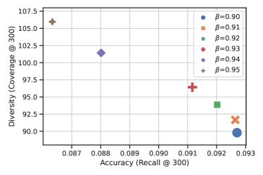
Figure 5. Accuracy-diversity trade-off by loss reweighting.

4.3.3. Hyper-parameter $\sigma$ and $k$

$\sigma$ and $k$ are introduced in Section 3.2. $k$ is the budget for neighbor selection, and $\sigma$ is used to compute the pair-wise similarity of neighbors. Experimental results are shown in Figure 6.

We can observe that DGRec is not that sensitive to $\sigma$. DGRec has a stable good performance on both Recall@300 and Coverage@300 with $\sigma$ varies from $0.01$ to $100$. With different $\sigma$, we can also see the trade-off between accuracy/diversity. When Coverage@300 achieves the best at $10$, Recall@300 is the worst.

$k$ is the number of neighbors for GNN aggregation. Neighbors are selected by submodular function to maximize diversity. As we can see from Figure 6, Recall@300 gradually decreases, and Coverage@300 increases with the increase of $k$. Submodular neighbor selection selects a diversified subset of neighbors. With a larger set, DGRec can aggregate from more diversified neighbors, which would lead to an increase in diversity. At the same time, accuracy would drop as a trade-off. We can also observe that Recall@300 does not drop much with the increase in diversity.

Experiments on $\sigma$ and $k$ show DGRec is not sensitive to the submodular selection module, and DGRec would not have a dramatic change because of this module. Meanwhile, this module can also balance accuracy and diversity by $\sigma$ and $k$.

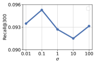
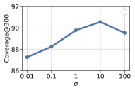
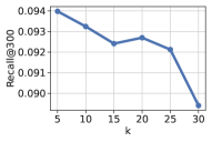
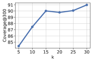
Figure 6. Parameter sensitivity of $\sigma$ and $k$. $\sigma$ controls the similarity computation and $k$ is the number of selected neighbors.

4.4. Ablation Study (RQ3)

In this section, we perform an ablation study on the TaoBao dataset by removing each of the three modules. Experiment results are shown in Table 4. We can have the following observations:

• The intact DGRec achieves the best C@300. The combination of proposed modules can effectively increase diversity.

• When we remove the submodular neighbor selection module, C@300 drops from $89.1684$ to $84.9129$ while there is only a tiny difference on Recall@300 and HR@300. It shows the submodular neighbor selection module can increase the diversity with minimal cost on accuracy.

• When we remove the layer attention module, C@300 decreases with the increase on R@300 and HR@300. It indicates layer attention balances accuracy and diversity.

• When we remove the loss reweighting module, R@300, HR@300, and C@300 all drop greatly. The loss reweighting module has the largest impact on DGRec because it not only balances the training on long-tail categories but also guides the learning of layer attention.

Table 4. Ablation study on TaoBao dataset. We show DGRec’ performance when removing each of the modules.

Method	R@300	HR@300	C@300
DGRec	0.0951	0.4817	89.1684
w/o Submodular selection	0.0982	0.4869	84.9129
w/o Layer attention	0.1009	0.4976	82.9553
w/o Loss reweighting	0.0886	0.4612	79.3286

4.5. Choice of Submodular Functions (RQ4)

In this section, we compare the influence of different submodular functions on model performance. We use two commonly used submodular functions to replace the facility location function. Experimental results are shown in Figure 7. Model A utilizes bucket coverage submodular function (Wei et al., 2015). Before selection, it clusters on each dimension and divides each dimension into buckets. The submodular function counts the gain on covered buckets. Model B utilizes category coverage submodular function (Wei et al., 2015). This function counts the gain on covered categories. Model C is DGRec, which utilizes the facility location function. Among the three models, model A and model C do not need item category information. They directly select neighbors based on neighbor embedding. Model B needs item category information to be able to compute category coverage gain during each selection.

From Figure 7, we observe that compared with the other two models, model A has much higher performance on Recall@300 and much lower performance on Coverage@300. It shows the selection of submodular functions has an influential impact on performance. Model B and model C achieve similar results with respect to Recall@300 and Coverage@300. It indicates the embedding learned by model C can accurately capture the category information, and the facility location function enlarges the category coverage during neighbor selection. We select the facility location function in DGRec for two reasons. Firstly, it can nearly achieve the best diversity compared with other methods. Secondly, it does not need category information during aggregation, which can enlarge the application scenarios when the category information is unobserved.

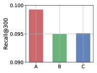
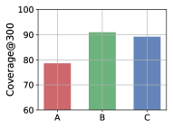
Figure 7. The influence of different submodular functions. A: bucket coverage function, B: category coverage function, and C: facility location function.

5. Related Work

In this section, we introduce the related work of DGRec, which includes Graph Neural Network based recommender system and diversified recommendation.

5.1. Graph Neural Network based Recommender System

With GNN showing excellent performance on graph-structured data, GNN-based recommender systems (Wang et al., 2021) are attracting more and more attention. These methods represent the user’s historical interactions as a user-item bipartite graph with easy access to high-order connectivity. GCMC (Berg et al., 2017) utilizes encoder-decoder structure on graph to complete interaction matrix. SpectralCF (Zheng et al., 2018) is the first to study the spectral domain of the user-item bipartite graph. It proposes spectral convolution operation to find the latent interactions, and greatly increase the recommendation performance on cold-start items. PinSAGE (Ying et al., 2018) designs a special random walk to accelerate the learning on the large-scale bipartite graph, which is applied on the Pinterest platform. NGCF (Wang et al., 2019) directly aggregates information from neighbors in the bipartite graph, and explicitly injects the collaborative signal in the learned embedding. LightGCN (He et al., 2020) simplifies NGCF by removing the overhead computation of linear transformation and non-linear activation. The simplified operation not only achieves better performance but also reduces the training time. UltraGCN (Mao et al., 2021) takes a further step in simplifying graph convolutional network. It skips the finite layers of aggregation, and directly computes the infinite convolution stage as a constraint during training. MetaKRec (Yang et al., 2022c) reconstructs the knowledge graph as edges between items before graph convolution.

Previous GNN-based recommender systems nearly all focus on increasing accuracy while leading to poor diversity. DGRec is also built upon Graph Neural Network. The proposed three modules can be added to previous GNN-based recommender systems and make up for their diversity shortcomings.

5.2. Diversified Recommendation

Diversified recommendation aims to recommend users with a diversified subset of items to help users find unexplored interests. Diversified recommendation is first proposed by Ziegler et al. (2005). They use a greedy method to select items during the retrieval procedure. Zhou et al. (2010) points out the accuracy/diversity dilemma, and propose HeatS/ProbS methods to choose the information propagation probability for each edge in the user/item bipartite graph.  Cheng et al. (2017) introduced a new pairwise accuracy metric and a normalized topic coverage diversity metric to measure the performance of accuracy and diversity. Then several re-ranking-based methods are proposed to diversify recommendation lists after the retrieval procedure. DUM (Ashkan et al., 2015) uses the submodular function to greedy guide the selection of item selection in the re-ranking procedure to maximize the item’s utility. Diversified PMF (Sha et al., 2016) computes $l_{2}$ loss between items as diversity. Determinantal point process (DPP) (Chen et al., 2018b) re-ranks items to achieve the largest determinant on the item’s similarity matrix. Antikacioglu and Ravi (2017) formulate a recommender system as a subgraph selection problem from diversified super graphs, and they use minimum-cost network flow methods to achieve a fast algorithm in diversification. Teo et al. (2016) assign global/local diversification weights in the training of recommender systems. CB2CF (Huang et al., 2021) designs sliding spectrum decomposition to capture user’s diversity perception over long item lists. Through online testing, CB2CF shows diversification can increase the number of engagements and time spent on the Xiaohongshu platform. DDGraph (Ye et al., 2021) selects implicit edges by quantile progressive candidate selection and re-constructs the user-item bipartite graph to increase diversity. DGCN (Zheng et al., 2021) is the first GNN-based diversified recommendation method. It selects node neighbors based on the inverse category frequency for diverse aggregation and further utilizes category-boosted negative sampling and adversarial learning to diverse items in the embedding space.

DGRec focuses on diversifying the GNN-based recommender system in the retrieval stage. Among the previous methods, the re-ranking-based methods such as DPP and DUM are compatible with our method. DGCN is the most similar work with DGRec. We both focus on how to increase diversity on GNN-based methods.

6. Conclusions

In this paper, we target diversifying GNN-based recommender systems with diversified embedding generation. We design three modules that can be easily applied to GNN-based recommender systems to achieve diversification with minimal cost on accuracy. Based on the three modules, we propose DGRec. When considering diversity, it surpasses the state-of-the-art diversified recommender system. It also achieves comparable accuracy with the most advanced accuracy-based recommender system. DGRec enables the trade-off between accuracy and diversity by several hyper-parameters. Extensive experiments on real-world datasets illustrate the influence of different modules.

- (1)
- Antikacioglu and Ravi (2017) Arda Antikacioglu and R Ravi. 2017. Post processing recommender systems for diversity. In Proceedings of the 23rd ACM SIGKDD International Conference on Knowledge Discovery and Data Mining. 707–716.
- Ashkan et al. (2015) Azin Ashkan, Branislav Kveton, Shlomo Berkovsky, and Zheng Wen. 2015. Optimal greedy diversity for recommendation. In Twenty-Fourth International Joint Conference on Artificial Intelligence.
- Berg et al. (2017) Rianne van den Berg, Thomas N Kipf, and Max Welling. 2017. Graph convolutional matrix completion. arXiv preprint arXiv:1706.02263 (2017).
- Carbonell and Goldstein (1998) Jaime Carbonell and Jade Goldstein. 1998. The use of MMR, diversity-based reranking for reordering documents and producing summaries. In Proceedings of the 21st ACM SIGIR conference on Research and development in information retrieval. 335–336.
- Chen et al. (2018b) Laming Chen, Guoxin Zhang, and Eric Zhou. 2018b. Fast greedy map inference for determinantal point process to improve recommendation diversity. Advances in Neural Information Processing Systems 31 (2018).
- Chen et al. (2018a) Yian Chen, Xing Xie, Shou-De Lin, and Arden Chiu. 2018a. WSDM cup 2018: Music recommendation and churn prediction. In Proceedings of the Eleventh ACM International Conference on Web Search and Data Mining. 8–9.
- Cheng et al. (2017) Peizhe Cheng, Shuaiqiang Wang, Jun Ma, Jiankai Sun, and Hui Xiong. 2017. Learning to Recommend Accurate and Diverse Items. In Proceedings of the 26th International Conference on World Wide Web. 183–192.
- Cornuejols et al. (1977) Gerard Cornuejols, Marshall Fisher, and George L Nemhauser. 1977. On the uncapacitated location problem. In Annals of Discrete Mathematics. Vol. 1. Elsevier, 163–177.
- Cui et al. (2019) Yin Cui, Menglin Jia, Tsung-Yi Lin, Yang Song, and Serge Belongie. 2019. Class-balanced loss based on effective number of samples. In Proceedings of the IEEE/CVF conference on computer vision and pattern recognition. 9268–9277.
- Gao et al. (2021) Weihao Gao, Xiangjun Fan, Chong Wang, Jiankai Sun, Kai Jia, Wenzi Xiao, Ruofan Ding, Xingyan Bin, Hui Yang, and Xiaobing Liu. 2021. Learning An End-to-End Structure for Retrieval in Large-Scale Recommendations. In Proceedings of the 30th ACM International Conference on Information & Knowledge Management. 524–533.
- Ge et al. (2020) Yingqiang Ge, Shuya Zhao, Honglu Zhou, Changhua Pei, Fei Sun, Wenwu Ou, and Yongfeng Zhang. 2020. Understanding echo chambers in e-commerce recommender systems. In Proceedings of the 43rd international ACM SIGIR conference on research and development in information retrieval. 2261–2270.
- Gu et al. (2020) Yulong Gu, Zhuoye Ding, Shuaiqiang Wang, and Dawei Yin. 2020. Hierarchical user profiling for e-commerce recommender systems. In Proceedings of the 13th International Conference on Web Search and Data Mining. 223–231.
- He et al. (2021) Chaoyang He, Keshav Balasubramanian, Emir Ceyani, Carl Yang, Han Xie, Lichao Sun, Lifang He, Liangwei Yang, Philip S Yu, Yu Rong, et al. 2021. Fedgraphnn: A federated learning system and benchmark for graph neural networks. arXiv preprint arXiv:2104.07145 (2021).
- He et al. (2020) Xiangnan He, Kuan Deng, Xiang Wang, Yan Li, Yongdong Zhang, and Meng Wang. 2020. Lightgcn: Simplifying and powering graph convolution network for recommendation. In Proceedings of the 43rd International ACM SIGIR conference on research and development in Information Retrieval. 639–648.
- Hoi et al. (2006) Steven CH Hoi, Rong Jin, Jianke Zhu, and Michael R Lyu. 2006. Batch mode active learning and its application to medical image classification. In ICML.
- Huang et al. (2021) Yanhua Huang, Weikun Wang, Lei Zhang, and Ruiwen Xu. 2021. Sliding Spectrum Decomposition for Diversified Recommendation. In Proceedings of the 27th ACM SIGKDD Conference on Knowledge Discovery & Data Mining. 3041–3049.
- Kingma and Ba (2014) Diederik P Kingma and Jimmy Ba. 2014. Adam: A method for stochastic optimization. arXiv preprint arXiv:1412.6980 (2014).
- Kipf and Welling (2017) Thomas N. Kipf and Max Welling. 2017. Semi-Supervised Classification with Graph Convolutional Networks. In 5th International Conference on Learning Representations, ICLR 2017.
- Liang et al. (2018) Jiongqian Liang, Peter Jacobs, Jiankai Sun, and Srinivasan Parthasarathy. 2018. Semi-supervised Embedding in Attributed Networks with Outliers. In Proceedings of the 2018 SIAM International Conference on Data Mining (SDM). 153–161.
- Liang et al. (2021) Yile Liang, Tieyun Qian, Qing Li, and Hongzhi Yin. 2021. Enhancing domain-level and user-level adaptivity in diversified recommendation. In Proceedings of the 44th International ACM SIGIR Conference on Research and Development in Information Retrieval. 747–756.
- Liu et al. (2022a) Kay Liu, Yingtong Dou, Yue Zhao, Xueying Ding, Xiyang Hu, Ruitong Zhang, Kaize Ding, Canyu Chen, Hao Peng, Kai Shu, Lichao Sun, Jundong Li, George H. Chen, Zhihao Jia, and Philip S. Yu. 2022a. BOND: Benchmarking Unsupervised Outlier Node Detection on Static Attributed Graphs. arXiv preprint arXiv:2206.10071 (2022).
- Liu et al. (2020) Meng Liu, Hongyang Gao, and Shuiwang Ji. 2020. Towards deeper graph neural networks. In Proceedings of the 26th ACM SIGKDD international conference on knowledge discovery & data mining. 338–348.
- Liu et al. (2021) Yonghao Liu, Renchu Guan, Fausto Giunchiglia, Yanchun Liang, and Xiaoyue Feng. 2021. Deep attention diffusion graph neural networks for text classification. In Proceedings of the 2021 Conference on Empirical Methods in Natural Language Processing. 8142–8152.
- Liu et al. (2022b) Zhiwei Liu, Liangwei Yang, Ziwei Fan, Hao Peng, and Philip S Yu. 2022b. Federated social recommendation with graph neural network. ACM Transactions on Intelligent Systems and Technology (TIST) 13, 4 (2022), 1–24.
- Mao et al. (2021) Kelong Mao, Jieming Zhu, Xi Xiao, Biao Lu, Zhaowei Wang, and Xiuqiang He. 2021. UltraGCN: ultra simplification of graph convolutional networks for recommendation. In Proceedings of the 30th ACM International Conference on Information & Knowledge Management. 1253–1262.
- Mayer-Schönberger and Cukier (2013) Viktor Mayer-Schönberger and Kenneth Cukier. 2013. Big data: A revolution that will transform how we live, work, and think. Houghton Mifflin Harcourt.
- Nemhauser et al. (1978) George L Nemhauser, Laurence A Wolsey, and Marshall L Fisher. 1978. An analysis of approximations for maximizing submodular set functions—I. Mathematical programming 14, 1 (1978), 265–294.
- Puthiya Parambath et al. (2016) Shameem A Puthiya Parambath, Nicolas Usunier, and Yves Grandvalet. 2016. A coverage-based approach to recommendation diversity on similarity graph. In Proceedings of the 10th ACM Conference on Recommender Systems. 15–22.
- Rendle et al. (2012) Steffen Rendle, Christoph Freudenthaler, Zeno Gantner, and Lars Schmidt-Thieme. 2012. BPR: Bayesian personalized ranking from implicit feedback. arXiv preprint arXiv:1205.2618 (2012).
- Scarselli et al. (2008) Franco Scarselli, Marco Gori, Ah Chung Tsoi, Markus Hagenbuchner, and Gabriele Monfardini. 2008. The graph neural network model. IEEE transactions on neural networks 20, 1 (2008), 61–80.
- Sha et al. (2016) Chaofeng Sha, Xiaowei Wu, and Junyu Niu. 2016. A framework for recommending relevant and diverse items.. In IJCAI, Vol. 16. 3868–3874.
- Sun et al. (2012) Jiankai Sun, Shuaiqiang Wang, Byron J. Gao, and Jun Ma. 2012. Learning to Rank for Hybrid Recommendation. In Proceedings of the 21st ACM International Conference on Information and Knowledge Management. 2239–2242.
- Teo et al. (2016) Choon Hui Teo, Houssam Nassif, Daniel Hill, Sriram Srinivasan, Mitchell Goodman, Vijai Mohan, and SVN Vishwanathan. 2016. Adaptive, personalized diversity for visual discovery. In Proceedings of the 10th ACM conference on recommender systems. 35–38.
- Wang et al. (2021) Shoujin Wang, Liang Hu, Yan Wang, Xiangnan He, Quan Z. Sheng, Mehmet A. Orgun, Longbing Cao, Francesco Ricci, and Philip S. Yu. 2021. Graph Learning based Recommender Systems: A Review. In Proceedings of the Thirtieth International Joint Conference on Artificial Intelligence. 4644–4652.
- Wang et al. (2012) Shuaiqiang Wang, Jiankai Sun, Byron J. Gao, and Jun Ma. 2012. Adapting Vector Space Model to Ranking-Based Collaborative Filtering. In Proceedings of the 21st ACM International Conference on Information and Knowledge Management. 1487–1491.
- Wang et al. (2014) Shuaiqiang Wang, Jiankai Sun, Byron J. Gao, and Jun Ma. 2014. VSRank: A Novel Framework for Ranking-Based Collaborative Filtering. ACM Trans. Intell. Syst. Technol. 5, 3 (2014).
- Wang et al. (2019) Xiang Wang, Xiangnan He, Meng Wang, Fuli Feng, and Tat-Seng Chua. 2019. Neural graph collaborative filtering. In Proceedings of the 42nd international ACM SIGIR conference on Research and development in Information Retrieval. 165–174.
- Wang et al. (2022) Yu Wang, Hengrui Zhang, Zhiwei Liu, Liangwei Yang, and Philip S Yu. 2022. ContrastVAE: Contrastive Variational AutoEncoder for Sequential Recommendation. In Proceedings of the 31st ACM International Conference on Information & Knowledge Management. 2056–2066.
- Wei et al. (2015) Kai Wei, Rishabh Iyer, and Jeff Bilmes. 2015. Submodularity in data subset selection and active learning. In International conference on machine learning. 1954–1963.
- Wu et al. (2019) Chuhan Wu, Fangzhao Wu, Mingxiao An, Jianqiang Huang, Yongfeng Huang, and Xing Xie. 2019. NPA: neural news recommendation with personalized attention. In Proceedings of the 25th ACM SIGKDD international conference on knowledge discovery & data mining. 2576–2584.
- Yang et al. (2021) Liangwei Yang, Zhiwei Liu, Yingtong Dou, Jing Ma, and Philip S Yu. 2021. Consisrec: Enhancing gnn for social recommendation via consistent neighbor aggregation. In Proceedings of the 44th international ACM SIGIR conference on Research and development in information retrieval. 2141–2145.
- Yang et al. (2022a) Liangwei Yang, Zhiwei Liu, Yu Wang, Chen Wang, Ziwei Fan, and Philip S Yu. 2022a. Large-scale Personalized Video Game Recommendation via Social-aware Contextualized Graph Neural Network. In Proceedings of the ACM Web Conference 2022. 3376–3386.
- Yang et al. (2022c) Liangwei Yang, Shen Wang, Jibing Gong, Shaojie Zheng, Shuying Du, Zhiwei Liu, and Philip S Yu. 2022c. MetaKRec: Collaborative Meta-Knowledge Enhanced Recommender System. arXiv preprint arXiv:2211.07104 (2022).
- Yang et al. (2022b) Mingdai Yang, Zhiwei Liu, Liangwei Yang, Xiaolong Liu, Chen Wang, Hao Peng, and Philip S Yu. 2022b. Ranking-based Group Identification via Factorized Attention on Social Tripartite Graph. arXiv preprint arXiv:2211.01830 (2022).
- Ye et al. (2021) Rui Ye, Yuqing Hou, Te Lei, Yunxing Zhang, Qing Zhang, Jiale Guo, Huaiwen Wu, and Hengliang Luo. 2021. Dynamic graph construction for improving diversity of recommendation. In Fifteenth ACM Conference on Recommender Systems. 651–655.
- Ying et al. (2018) Rex Ying, Ruining He, Kaifeng Chen, Pong Eksombatchai, William L Hamilton, and Jure Leskovec. 2018. Graph convolutional neural networks for web-scale recommender systems. In Proceedings of the 24th ACM SIGKDD international conference on knowledge discovery & data mining. 974–983.
- Zheng et al. (2014) Jingjing Zheng, Zhuolin Jiang, Rama Chellappa, and Jonathon P Phillips. 2014. Submodular Attribute Selection for Action Recognition in Video. In NIPS.
- Zheng et al. (2018) Lei Zheng, Chun-Ta Lu, Fei Jiang, Jiawei Zhang, and Philip S Yu. 2018. Spectral collaborative filtering. In Proceedings of the 12th ACM conference on recommender systems. 311–319.
- Zheng et al. (2021) Yu Zheng, Chen Gao, Liang Chen, Depeng Jin, and Yong Li. 2021. DGCN: Diversified Recommendation with Graph Convolutional Networks. In Proceedings of the Web Conference 2021. 401–412.
- Zhou et al. (2010) Tao Zhou, Zoltán Kuscsik, Jian-Guo Liu, Matúš Medo, Joseph Rushton Wakeling, and Yi-Cheng Zhang. 2010. Solving the apparent diversity-accuracy dilemma of recommender systems. Proceedings of the National Academy of Sciences 107, 10 (2010), 4511–4515.
- Ziegler et al. (2005) Cai-Nicolas Ziegler, Sean M McNee, Joseph A Konstan, and Georg Lausen. 2005. Improving recommendation lists through topic diversification. In Proceedings of the 14th international conference on World Wide Web. 22–32.