Compiling Structured Tensor Algebra

Abstract.

Tensor algebra is essential for data-intensive workloads in various computational domains. Computational scientists face a trade-off between the specialization degree provided by dense tensor algebra and the algorithmic efficiency that leverages the structure provided by sparse tensors. This paper presents StructTensor, a framework that symbolically computes structure at compilation time. This is enabled by Structured Tensor Unified Representation (STUR), an intermediate language that can capture tensor computations as well as their sparsity and redundancy structures. Through a mathematical view of lossless tensor computations, we show that our symbolic structure computation and the related optimizations are sound. Finally, for different tensor computation workloads and structures, we experimentally show how capturing the symbolic structure can result in outperforming state-of-the-art frameworks for both dense and sparse tensor algebra.

1. Introduction

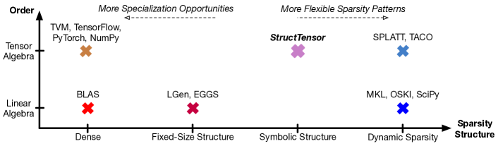
Figure 1. Comparison of different linear and tensor algebra frameworks.

Linear and tensor algebra operations are the key drivers of data-intensive computations in many domains, such as physics simulations (Martín-García, 2008; Ran et al., 2020), computational chemistry (Titov et al., 2013; Hirata, 2006), bioinformatics (Cichocki et al., 2009), and deep learning (Smith and Gray, 2018; Hirata, 2003). Due to their importance, many specialization attempts have been made throughout the entire system stack from hardware to software layers. The tensor accelerators (Hegde et al., 2019) and TPUs (Jouppi et al., 2017) provide efficient tensor processing at the hardware level. On the software level, there have been advances in providing highly-tuned kernels (Dongarra et al., 1990), as well as compilation frameworks that globally optimize tensor computations (Gareev et al., 2018).

There is a trade-off for using tensor algebra frameworks between the specialization degree and the flexibility of the structure such as sparsity (Figure 1). On the one side of the spectrum, extensive research has been done on dense tensors without leveraging any structure. Such tensors appear in deep neural networks and computational physics. As all the memory access patterns are known at compilation time, one can provide heavily-tuned implementations without any knowledge about the content of tensors. As a result, the high-performance engineer or compiler has enough reasoning power to make decisions on parallelization, vectorization, and tiling.

However, many real-world applications involve tensors that exhibit symmetries and, more generally, specific structures which can be exploited to significantly reduce computational costs. Sparse tensor algebra for instance only captures the pattern of zero/non-zero elements in tensors during runtime, and has been at the center of recent interest (Strout et al., 2018; Kjolstad et al., 2017). However, postponing the memory access patterns to the runtime hinders the specialization power of the compiler (Augustine et al., 2019). As a partial remedy, there have been efforts (Tang et al., 2020; Spampinato and Püschel, 2016) to statically determine the structure of matrices during the compilation time. However, these are limited to fixed-size matrices.

To resolve the dilemma between using tensor algebra frameworks focusing on either dense or sparse tensors (Figure 1), this paper introduces StructTensor. StructTensor captures the structure of tensors symbolically at compilation time. On the one hand, the underlying compiler can use this symbolic information to specialize the code at the level of dense computations. On the other hand, the compiler can leverage this symbolic information in order to eliminate unnecessary and redundant computation.

In StructTensor, all tensor computations and structure information are translated to a single intermediate language called Structured Tensor Unified Representation (STUR). STUR propagates the structure knowledge throughout the computation at compile time. This is followed by efficient C++ code generation.

Specifically, we make the following contributions:

• We present StructTensor, the first framework that supports structured computation for tensor algebra (Section 3). For a tensor $T$, the structure handled by StructTensor comes as a pair $(T_{U},T_{R})$, where

  • $T_{U}$ tracks the symbolic sparsity structure of the tensor,

  • $T_{R}$ tracks the redundancy structure, which captures symmetries and repetition patterns.

• We propose STUR, a unified intermediate representation (IR) that can express tensor computations. It allows capturing non-optimized tensors as well as their symbolic structures $T_{U},T_{R}$ in a single IR (Section 4).

• We show how StructTensor uses the structure information in its compilation process (Section 5). It leverages STUR and rewrites tensors in 3 steps (also see Figure 3):

  1. StructTensor propagates the structure information on the syntax tree of tensor computation (Section 5.1)

  2. Several optimizations are applied to the unified representation for tensor computations and their structure leading to computation over a compressed tensor (Section 5.2)

  3. StructTensor generates C++ code for the tensor computation over the compressed form, as well as reconstructing the uncompressed tensor (Section 5.5)

• We give a mathematical view on the problem of lossless tensor computations that we study in this paper, and show the soundness of our rewrites and structure inference in Section 6.

• We experimentally evaluate StructTensor for different tensor computation workloads and structures (Section 7). We show that StructTensor can leverage the structure of tensors to generate computation over compressed tensors in order to outperform state-of-the-art dense and sparse tensor computation frameworks.

2. Background

Structured Linear Algebra. There are several well-known structures for matrices, such as diagonal, symmetric, and lower/upper triangular, that considering them while doing calculations over matrices can reduce computational time. Figure 2 represents a set of linear algebra operations and well-known matrix structures.

Example - Diagonal Matrices. Imagine the case of the Kronecker product between two diagonal matrices $A_{n\times n}$ and $B_{m\times m}$. Typically, the Kronecker product of these matrices is defined as:

(1) $$(A\otimes B)_{mr+v,ms+w}=A_{r,s}\cdot B_{v,w}$$

where the result dimension is $nm\times nm$. Therefore the computational cost would be $O(n^{2}m^{2})$. However, if the computation is structure-aware, one can leverage the fact that all non-zero elements are on the diagonal of matrices. Therefore, it is sufficient to perform the multiplication over only those elements, which results in the following computation:

(2) $$(A\otimes B)_{mr+v,mr+v}=A_{r,r}\cdot B_{v,v}$$

where the result is diagonal as well. As a result, the computational complexity for this Kronecker product reduces to $O(nm)$. Furthermore, since the structure of the result is known (diagonal), this information can be used in further computations efficiently. Figure 2 shows a subset of inference rules to determine the output structure based on input structures.

$e$ $::=$ $e\cdot e$ $\mid$ $e\odot e$ $\mid$ $e\otimes e$ $\mid$ $e+e$ $\mid$ $e\oplus e$ $\mid$ $e^{T}$ $\mathcal{G}$ General dense matrix $\mathcal{S}$ Symmetric matrix $\mathcal{D}$ Diagonal matrix $\mathcal{R}_{n}$ Matrix of non-zeros only at $n^{th}$ row $\mathcal{C}_{n}$ Matrix of non-zeros only at $n^{th}$ column $\mathcal{H}_{n,m}$ Singular matrix at index $n,m$ $\mathcal{Z}$ All zeros matrix

$e$: $\mathcal{C}_{n}$ $e\cdot e^{T}$: $\mathcal{S}$       $e_{1}$: $\mathcal{C}_{n}$    $e_{2}$: $\mathcal{R}_{m}$    $n\neq m$ $e_{1}\cdot e_{2}$: $\mathcal{Z}$ $e_{1}$: $\mathcal{C}_{n}$    $e_{2}$: $\mathcal{R}_{n}$ $e_{1}\cdot e_{2}$: $\mathcal{G}$       $e_{1}$: $\mathcal{R}_{n}$    $e_{2}$: $\mathcal{C}_{m}$ $e_{1}\times e_{2}$: $\mathcal{H}_{n,m}$ $e_{1}$: $\mathcal{R}_{n}$    $e_{2}$: $\mathcal{R}_{m}$ $e_{1}\cdot e_{2}$: $\mathcal{R}_{n}$       $e_{1}$: $\mathcal{C}_{n}$    $e_{2}$: $\mathcal{C}_{m}$ $e_{1}\cdot e_{2}$: $\mathcal{C}_{m}$ $e_{1}$: $\mathcal{D}$    $e_{2}$: $\mathcal{D}$ $e_{1}\odot e_{2}$: $\mathcal{D}$       $e_{1}$: $\mathcal{D}$    $e_{2}$: $\mathcal{D}$ $e_{1}\otimes e_{2}$: $\mathcal{D}$ $e_{1}$: $\mathcal{D}$    $e_{2}$: $\mathcal{D}$ $e_{1}\cdot e_{2}$: $\mathcal{D}$       $e_{1}$: $\mathcal{D}$    $e_{2}$: $\mathcal{D}$ $e_{1}\oplus e_{2}$: $\mathcal{D}$

Figure 2. The grammar for structured linear algebra operations and a subset of structure inference rules.

Sparsity and Redundancy Structures. Structures that distinguish zero and non-zero values are referred to as sparsity structures, such as diagonal and lower/upper triangular. Other structures like symmetric can capture redundancy patterns and are thus referred to as redundancy structures. Because of the redundancy pattern, it is possible to reconstruct the whole matrix by storing half of the data even though they are non-zero. Knowing and propagating structures in many cases helps reduce computational costs (Spampinato and Püschel, 2016).

Intricate Structures. The aforementioned structures cannot cover more complicated patterns. Imagine the case of creating the covariance matrix for the polynomial regression degree two model. Figure 4 shows the covariance matrix created for a polynomial degree two model on a data element with 4 features. Each number and color is associated with distinct elements, and elements with the same number have the same value. As it is represented in Figure 4, there are only 65 distinct elements even though the covariance matrix dimension is $20\times 20$. The redundancy pattern in this matrix is sophisticated and cannot be captured using the existing structures. Utilizing such structure information enhances the performance of machine learning tasks that require covariance matrix creation such as training polynomial regression models.

Tensor Structures. The complicated structure of the mentioned covariance matrix can be captured in the form of a higher-order tensor structure. This covariance matrix contains all degree-2, degree-3, and degree-4 interactions between features in itself. The reason that redundancy happens is that these interactions are computed multiple times. For example, degree-2 interactions inside the matrix form a symmetric structure. Degree-3 and degree-4 interactions have some complex forms of redundancy as well as being symmetric. These interactions cover all the elements inside the covariance matrix. By representing degree $i$ interactions as a tensor of order-$i$, the computation can be done more efficiently. This way, the only unique elements in degree two, three, and four tensors $T2(i,j),T3(i,j,k),T4(i,j,k,l)$ reside in $\{T2(i,j)\mid 1\leq i\leq j\leq n\},\{T3(i,j,k)\mid 1\leq i\leq j\leq k\leq n\},\{T4(i,j,k,l)\mid 1\leq i\leq j\leq k\leq l\leq n\}$ respectively. This structure in the new data format forms a generalized symmetric pattern that is easy to capture and leads to efficient computation. In the following sections, it is explained how StructTensor handles sophisticated structures and generates efficient C++ code for the computations.

3. Overview

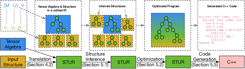
Figure 3. StructTensor architecture overview.

In this section, the overall architecture of StructTensor is described (cf. Figure 3).

Input. StructTensor gets linear algebra and tensor algebra expressions and the structure of their parameters as input. These operations and structures subsume the ones that are mentioned in Figure 2. All tensor expressions, as well as their structures, are represented in the StructTensor unified representation, called STUR. Sparsity and redundancy structures are captured in a unique set and redundancy map, respectively. The unique set contains unique and non-zero elements, and the redundancy map has the mapping from redundant and non-zero elements outside the unique set to their corresponding value in the unique set. These two subsume SInfo and AInfo used in LGen (Spampinato and Püschel, 2016) to model structured matrices.

Structure Inference. Afterward, we infer the structure of the intermediate and output tensor expressions by propagating the structure through STUR. A predefined set of inference rules for operations and structures is provided in STUR. The output structure is inferred in terms of the unique set and redundancy map by using inference rules. The inference rules set is extensible to cover arbitrary operations and structures as well.

Optimizations. Various optimizations are applied to STUR expressions. Throughout the structure inference process, several intermediate unique sets and redundancy maps are created. The tensor inlining optimization removes intermediate sets and maps. Moreover, input structures and previous optimizations by STUR can produce repetitive conditions over iterators. Through logical simplifications, only distinct conditions are kept for the code generation step.

Code Generation. Finally, the optimized STUR is fed to the C++ code generator. The code generator assumes an order for iterators, calculates loop nest boundaries, and generates an efficient structure-aware C++ code. The generated code performs the computations over compressed format with lower computational cost thanks to the unique set. By utilizing the redundancy map, the final output tensor can be reconstructed for the user.

Example - Polynomial Regression Degree-2. We consider the creation of a covariance matrix for polynomial regression degree-2. The covariance matrix for an element with $n$ features is defined as:

$\Sigma(\mathbf{x})=\mathbf{x}\cdot\mathbf{x}^{T}=\mathbf{x}\otimes\mathbf{x}$

This represents the outer product of $\mathbf{x}$ with itself, and thus can be represented using the vector outer product operation $\otimes$. The vector $\mathbf{x}$ is a vector resulting from the concatenation of the feature vector $\mathbf{f}$ with the vector resulting from the interaction of the features. In terms of linear algebra, this is expressed as:

$\mathbf{x}=\mathbf{f}\oplus vec(\mathbf{f}\otimes\mathbf{f})$

Here, $\oplus$ is the vector concatenation, $\otimes$ is the vector outer product, and $vec(M)$ flattens the matrix $M$ of size $n\times m$ into a vector of size $n\cdot m$. By inlining the definition of x and by using the identity for the distribution of vector concatenation and vector outer product, we have:

$\Sigma(\mathbf{x})$	$=$	$(\mathbf{f}\oplus vec(\mathbf{f}\otimes\mathbf{f}))$	$\otimes$	$(\mathbf{f}\oplus vec(\mathbf{f}\otimes\mathbf{f}))$
	$=$	$\big{(}(\mathbf{f}\otimes\mathbf{f})||(\mathbf{f}\otimes vec(\mathbf{f}\otimes\mathbf{f}))\big{)}$	$//$	$\big{(}(vec(\mathbf{f}\otimes\mathbf{f})\otimes\mathbf{f})||(vec(\mathbf{f}\otimes\mathbf{f})\otimes vec(\mathbf{f}\otimes\mathbf{f}))\big{)}$

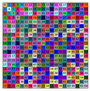
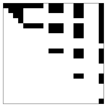
Figure 4. The covariance matrix of Polynomial Regression degree-2. Its redundancy pattern is shown on the left and its unique elements in compressed format are on the right.

The operations $||$ and $//$ correspond to matrix horizontal and vertical concatenation, respectively. StructTensor improves the performance for this computation in two levels of granularity. In a coarse-level of granularity, it detects that $(\mathbf{f}\otimes vec(\mathbf{f}\otimes\mathbf{f}))$ and $(vec(\mathbf{f}\otimes\mathbf{f})\otimes\mathbf{f})$ are computing the same elements but in a different layout. Thus, it only performs one of the computations and it would be sufficient to compute the following vector outer product terms:

$M1$	$=$	$\mathbf{f}\otimes\mathbf{f}$
$M2$	$=$	$\mathbf{f}\otimes vec(\mathbf{f}\otimes\mathbf{f})$
$M3$	$=$	$vec(\mathbf{f}\otimes\mathbf{f})\otimes vec(\mathbf{f}\otimes\mathbf{f})$

In a finer-level of granularity, for each of the terms $M1,M2,M3$, StructTensor detects a generalized symmetric structure. For $M1$ it detects a standard symmetric structure where it is sufficient to only keep the upper half of the matrix. For $M2$ and $M3$, there are $\sim 5\times$ and $\sim 23\times$ redundant elements, the patterns of which can be seen in Figure 4. After inferring such structures, StructTensor generates the following C++ code for each of these terms:

⬇ // Computation for M3 for(int i=0; i<n; ++i){ for(int j=i; j<n; ++j){ for(int k=j; k<n; ++k){ for(int l=k; l<n; ++l){ int r=i*n+j; int c=k*n+l; M3[r][c]=f[i]*f[j]*f[k]*f[l]; }}}}

Note that the nested iterations only cover a subset of the range.

In the next sections, we will thoroughly elaborate on how StructTensor works.

4. STUR: Structured Tensor Unified Language

In this section, the syntax of the unified intermediate representation, STUR, is represented. We elaborately explain the grammar for the unique set, redundancy map, and compressed tensor computation in this section. Moreover, details of how structured linear algebra is represented in STUR can be found in this section.

Program	${p}$	$::=$	${r}$ $\mid$ ${r}$; ${p}$	List of rules.
Rule	${r}$	$::=$	$A$ $:=$ $B$	Head (access) and body (Sum of Products).
Body	$B$	$::=$	${f}$ $\mid$ ${f}$ $+$ $B$	Sum of factor products.
Factor	${f}$	$::=$	${e}$ $\mid$ ${e}$ $*$ ${f}$	Product of expressions.
Expression	${e}$	$::=$	${x}$ $\theta$ ${i}$ $\mid$ ${i}$ $\theta$ ${x}$ $\mid$ $A$	Comparison ($\theta$) or access.
Index	${i}$	$::=$	${x}$ $\mid$ ${c}$ $\mid$ ${i}$ $\diamond$ ${i}$	Variable, constant, or arithmetic ($\diamond$) over indices.
Access	$A$	$::=$	$T$($\overline{\text{${x}$}}$) $\mid$ $T$C($\overline{\text{${x}$}}$) $\mid$	Tensor, compressed tensor,
			$T$U($\overline{\text{${x}$}}$) $\mid$ $T$R($\overline{\text{${x}$}}$)	unique set, and redundancy map access.

Figure 5. Grammar of STUR. The meta variables ${x}$ and $T$ range over the name of index variables and tensors, respectively.

4.1. The syntax of STUR

Grammar. Figure 5 shows STUR grammar which covers the grammar for tensor, unique set, and redundancy map computations. Each program ($P$) is made of several rules ($R$). Each rule is in the form of an assignment from a body ($B$) to an access to a collection ($A$). The collection could be a tensor ($T$), compressed tensor ($T$_C), unique set ($T$_U), or redundancy map ($T$_R), whereas the access index can be multiple index variables ($\overline{X}$), an index variable, or a constant value. The assignment body is represented as a sum of factor products ($F$). Each factor restricts the domain of values that an index variable can have. This is achieved through a collection access or a comparison term.

Example - Simple Tensor Operation. Consider the following STUR program:

$T_{3}(x,y)$	$:=$	$T_{1}(x,y)*T_{2}(x,y)$
$T_{4}(x)$	$:=$	$T_{3}(x,y)*(x=y)$

This program consists of two rules, with two input tensors $T_{1}$ and $T_{2}$. The first rule constructs the tensor $T_{3}$ of order-2, i.e., a matrix, which is computed by performing an element-wise multiplication of the two input matrices. The second rule constructs an order-1 tensor, i.e., a vector, that contains the elements of the diagonal of the matrix $T_{3}$. This is achieved by (1) restricting the range of $x$ and $y$ by the comparison term $x=y$, and (2) existentially quantifying over $y$ by not including it in the head of the rule.

Sum-of-Product Semantics. The addition and multiplication in STUR are defined based on the underlying collection; for unique sets and redundancy maps, the addition and multiplication are defined as set union and intersection, whereas for tensors and compressed tensors they are defined as real number addition and multiplication. Each rule can existentially quantify the free variables of the body by not including them in the rule head. This is known as marginalization in the AI community. All the free variables in the head should already be defined in the body (cf. Figure 6)

Syntactic Sugar. To simplify the presentation, we consider the following syntactic sugar, where $\bm{x}$ corresponds to a list of arguments $x_{1},\ldots,x_{k}$:

$(a\leq x<c)$	$\equiv$	$(a\leq x)*(x<c)$
$(x=y=z)$	$\equiv$	$(x=y)*(y=z)$
$\bm{x}\theta\bm{b}$	$\equiv$	$(x_{1}\theta b_{1})*\ldots*(x_{k}\theta b_{k})$

$T(x_{1},\ldots,x_{n}):=e$ $FV(T(x_{1},\ldots,x_{n}))\subseteq FV(e)$ $FV(T(x_{1},\ldots,x_{n}))=\{x_{1},\ldots,x_{n}\}$

$FV(e1+e2)=FV(e1)\cap FV(e2)$ $FV(e1*e2)=FV(e1)\cup FV(e2)$ $FV(t1\diamond t2)=FV(t1)\cup FV(t2)$

$FV(x\theta t)=\{x\}\cup FV(t)$ $FV(x)=\{x\}$ $FV(c)=\emptyset$

Figure 6. Free variable rules.

Unique sets. The sparsity structure of all the distinct elements of a tensor is encoded in a unique set. The grammar of STUR already captures the definition of unique sets (cf. Figure 5); a unique set is provided as a sum of products of comparison terms or access to other unique sets (and redundancy maps). Unique sets enhance performance by restricting index boundaries.

Example - Chess Pattern Unique Set. The following STUR specifies the unique set of a matrix $T$ of size $m\times n$ with a chess-board pattern for the sparsity:

$T_{U}(i,j)$	$:=$	$(0\leq i^{\prime}<(m/2))*(0\leq j^{\prime}<(n/2))*(i=i^{\prime}*2)*(j=j^{\prime}*2+1)$ $+$
		$(0\leq i^{\prime}<(m/2))*(0\leq j^{\prime}<(n/2))*(i=i^{\prime}*2+1)*(j=j^{\prime}*2)$

The first factor product specifies the elements of the even rows (that have an odd column index), and the second one specifies the ones for odd rows (with an even column index).

Redundancy Maps. The remaining non-zero elements which do not appear in the unique set domain are covered by the redundancy map. A redundancy map keeps the association between these elements’ indices and their corresponding indices in the unique set. Similar to the unique set, it is represented as a sum of products of comparison terms or access to other unique sets and redundancy maps. For a tensor of order-$k$, the redundancy map has $2k$ index variables. The first $k$ index variables correspond to the indices of the redundant element, whereas the second $k$ one corresponds to the indices from the unique set. The redundancy map enables the capability of reconstructing the full matrix from the compressed version that only contains unique elements. Restricting the computations to the elements of the unique set and reconstructing the uncompressed final result once, when all the calculation is over, can significantly improve the performance.

Example - Identical Row Matrix Redundancy Map. Consider a matrix $T$ of size $m\times n$, where all rows are the same. The unique set and redundancy maps for this matrix are defined as follows:

$T_{U}(i,j)$	$:=$	$(i=0)*(0\leq j<n)$
$T_{R}(i,j,i^{\prime},j^{\prime})$	$:=$	$(0<i<m)*(0\leq j<n)*(i^{\prime}=0)*(j^{\prime}=j)$

The first rule specifies that the unique elements are only in the first row ($i=0$). The first term of the second rule $(0<i<m)$ restricts the range of redundant elements to the ones from all the rows except the first one. The last two terms specify the index of the corresponding element from the unique set by specifying the first row ($i^{\prime}=0$) and the same column as the redundant element ($j^{\prime}=j$).

Compressed Tensor. StructTensor leverages the structure for better performance by representing the tensor in a lossless compressed format. This is achieved by combining the original tensor with the unique set in order to extract only the unique elements. The compressed tensor $T_{C}$ for the original tensor $T$ is defined as:

$T_{C}(\bm{x}):=T(\bm{x})*T_{U}(\bm{x})$

Naïvely executing the computation using this formula can even make the performance worse. After performing simplifications, the code generator produces code that iterates over the domain provided by the unique set for operations and excludes all the other elements of that tensor. This way, no extra computational cost is imposed while computing the result. When the computation is done, the uncompressed tensor $T$ is retrievable by using $T_{R}$.

Example - Upper Triangular Matrix Compressed Tensor. A $n\times n$ upper triangular matrix compressed tensor is calculated as follows:

$T_{U}(i,j)$	$:=$	$(0\leq i\leq j<n)$
$T_{C}(i,j)$	$:=$	$T(i,j)*(0\leq i\leq j<n)$

When $T(i,j)$ appears in a computation, the optimizer converts it to $T_{C}(i,j)$ and only uses elements with $0\leq i\leq j<n$. Therefore, only half of the elements are used in the computation, which leads to a $\sim 2\times$ speed up.

$\llbracket$$e^{T}$$\rrbracket$$(i,j)$ $:=$ $\llbracket$$e$$\rrbracket$$(j,i)$ $\llbracket$$e_{1}+e_{2}$$\rrbracket$$(i,j)$ $:=$ $\llbracket$$e_{1}$$\rrbracket$$(i,j)$ $+$ $\llbracket$$e_{2}$$\rrbracket$$(i,j)$ $\llbracket$$e_{1}\cdot e_{2}$$\rrbracket$$(i,j)$ $:=$ $\llbracket$$e_{1}$$\rrbracket$$(i,k)$ $*$ $\llbracket$$e_{2}$$\rrbracket$$(k,j)$ $\llbracket$$e_{1}\odot e_{2}$$\rrbracket$$(i,j)$ $:=$ $\llbracket$$e_{1}$$\rrbracket$$(i,j)$ $*$ $\llbracket$$e_{2}$$\rrbracket$$(i,j)$ $\llbracket$$e_{1}\otimes e_{2}$$\rrbracket$$(i,j)$ $:=$ $\llbracket$$e_{1}$$\rrbracket$$\big{(}i^{\prime},j^{\prime}\big{)}$ $+$ $\llbracket$$e_{2}$$\rrbracket$$\big{(}i^{\prime\prime},j^{\prime\prime}\big{)}$ where $(m,n)=dims(e_{2})$, $i^{\prime}=\big{\lfloor}$ $i/m$ $\big{\rfloor}$, $j^{\prime}=\big{\lfloor}$ $j/n$ $\big{\rfloor}$ $i^{\prime\prime}=i\%m$, $j^{\prime\prime}=j\%n$

$\llbracket$$e_{1}\oplus e_{2}$$\rrbracket$$(i,j)$ $:=$ $\llbracket$$e_{1}$$\rrbracket$$(i,j)$ $+$ $\llbracket$$e_{2}$$\rrbracket$ $\big{(}i^{\prime},j^{\prime}\big{)}$ where $(m,n)=dims(e_{1})$ $i^{\prime}=i-m$ , $j^{\prime}=j-n$ $\llbracket$$e_{1}\cdot e_{2}$$\rrbracket$$()$ $:=$ $\llbracket$$e_{1}$$\rrbracket$$(i)$ $*$ $\llbracket$$e_{2}$$\rrbracket$$(i)$ $\llbracket$$e_{1}+e_{2}$$\rrbracket$$(i)$ $:=$ $\llbracket$$e_{1}$$\rrbracket$$(i)$ $+$ $\llbracket$$e_{2}$$\rrbracket$$(i)$ $\llbracket$$e_{1}\oplus e_{2}$$\rrbracket$$(i)$ $:=$ $\llbracket$$e_{1}$$\rrbracket$$(i)$ $+$ $\llbracket$$e_{2}$$\rrbracket$ $\big{(}i^{\prime}\big{)}$ where $(n)=dims(e_{1})$, $i^{\prime}=i-n$ $\llbracket$$e_{1}\otimes e_{2}$$\rrbracket$$(i,j)$ $:=$ $\llbracket$$e_{1}$$\rrbracket$$(i)$ $*$ $\llbracket$$e_{2}$$\rrbracket$$(j)$

Figure 7. Representation of linear algebra operations in STUR. Here, $\cdot$ and $\otimes$ are overloaded; they correspond to matrix multiplication/Kronecker product for matrices and inner/outer product for vectors, respectively.

$e$: $\mathcal{Z}$

$T_{U}(i,j):=\emptyset$

$e$: $\mathcal{G}$

$T_{U}(i,j):=(0\leq i<m)*(0\leq j<n)$

$e$: $\mathcal{H}_{n1,n2}$     $0\leq n1<m$     $0\leq n2<n$

$T_{U}(i,j):=(i=n1)*(j=n2)$

$e$: $\mathcal{D}$     $m=n$

$T_{U}(i,j):=(0\leq i<n)*(i=j)$

$e$: $\mathcal{R}_{r}$     $0\leq r<m$
$T_{U}(i,j):=(i=r)*(0\leq j<n)$
$e$: $\mathcal{C}_{c}$     $0\leq c<n$
$T_{U}(i,j):=(0\leq i<m)*(j=c)$

$e$: $\mathcal{S}$           $m=n$
$T_{U}(i,j)$	$:=$	$(0\leq i\leq j<n)$
$T_{R}(i,j,i^{\prime},j^{\prime})$	$:=$	$(0\leq j<i<n)$ $*$
		$(i^{\prime}=j)*(j^{\prime}=i)$

Figure 8. Representation of well-known matrix structures in STUR. In all cases, $\llbracket$$e$$\rrbracket$$=T$ and thus $T_{U}$ and $T_{R}$ correspond to its unique set and redundancy map, respectively. Furthermore, we assume that $(m,n)=dims(e)$ for all cases and $T_{R}(i,j,i^{\prime},j^{\prime}):=\emptyset$ unless stated explicitly.

4.2. Translating Structured Linear Algebra to STUR

Operations. The representation of linear algebra operations is shown in Figure 7. Imagine the matrices $M_{1}$ and $M_{2}$ with dimensions $m_{1}\times n_{1}$ and $m_{2}\times n_{2}$ are represented in STUR as $\llbracket$$e_{1}$$\rrbracket$ and $\llbracket$$e_{2}$$\rrbracket$, respectively. The element in $i$-th row and $j$-th column of $M_{1}\mathbin{\vbox{\hbox{\scalebox{0.75}{$\bullet$}}}}M_{2}$ where $\mathbin{\vbox{\hbox{\scalebox{0.75}{$\bullet$}}}}$ is an operator is $\llbracket$$e_{1}\mathbin{\vbox{\hbox{\scalebox{0.75}{$\bullet$}}}}e_{2}$$\rrbracket$$(i,j)$. Each operation is translated to a sum of product format in STUR. For instance, if $\mathbin{\vbox{\hbox{\scalebox{0.75}{$\bullet$}}}}=\oplus$, then the direct sum of $M_{1}$ and $M_{2}$ is translated by the top-right rule in Figure 7. This rule specifies that element $(i,j)$ of the output is taken from $\llbracket$$e1$$\rrbracket$ when $i<m$ and $j<n$ and from $\llbracket$$e2$$\rrbracket$ when $i\geq m$ and $j\geq n$.

Structures. Figure 8 shows the representation of well-known matrix structures in STUR. Structures are translated to a combination of a unique set and a redundancy map. For example, if matrix $M$ has a symmetric structure, the upper triangular section of that is counted as the unique set. Therefore, the lower triangular region is considered as the redundant section; the redundancy map keeps the transformations from the lower triangular region to the corresponding upper region. Hence, if the representation of $M$ in STUR is $T$, the unique set and redundancy map are provided by the last rule of Figure 8. When $j<i$, according to $T_{R}(i,j,i^{\prime},j^{\prime})$, the values of $T(i,j)$ will be retrieved from values in $T(j,i)$.

5. Compilation

In this section, we show how StructTensor symbolically computes and propagates the structure. Optimizing the tensor computation using the inferred structure leads to structure-aware code generation.

5.1. Structure Inference

$T(\bm{x})$	$:=$	$M(\bm{y})*V(\bm{z})$     $\bm{x}=\bm{y}\cup\bm{z}$
$T_{U}(\bm{x})$	$:=$	$M_{U}(\bm{y})*V_{U}(\bm{z})$

$T(\bm{x})$	$:=$	$M(\bm{x})+V(\bm{x})$
$T_{U}(\bm{x})$	$:=$	$M_{U}(\bm{x})+V_{U}(\bm{x})$

$T(\bm{x})$	$:=$	$M(\bm{y})$     $\bm{x}\subseteq\bm{y}$
$T_{U}(\bm{x})$	$:=$	$M_{U}(\bm{y})$

Figure 9. Inference rules for unique set. Here we assume the redundancy maps of inputs are empty.

Inference for unique sets. Figure 9 shows the inference rules for the output structure. These rules follow the assumption that input redundancy maps are empty and only capture sparsity patterns. Since all operations are translated to multiplication, addition, or projection in STUR, providing inference rules only for these operations is sufficient. Moreover, having more than two operands is handled by breaking them into subexpressions with two operands and storing the results in intermediate sets.

In the case of multiplication, the result is non-zero only if both inputs are non-zero values. Having a zero operand in multiplication makes the final result zero. Therefore, the unique set of output is calculated from the intersection of non-zero elements in both operands. Addition on the other hand is non-zero even if one of the operands is non-zero. Hence, any element in the unique set of operands can lead to a non-zero element in output. Consequently, the unique set of output is the union over the unique set of its operands. Since projection is defined by summing up all values, it follows the same rule as addition. Any non-zero element in the unique set of the input can create a non-zero element in the output. So the output unique set for projection is computed by unioning over all unique set values in that dimension.

Example - Unique Set Computation. Consider the following tensor computation:

$A(i,j,k)$

$:=$

$B(i,j,l)*C(i,k)+D(j,k)*E(i,j)$

where input unique sets are

$B_{U}(i,j,l)$	$:=$	$i\leq j,$	$C_{U}(l,k)$	$:=$	$l=k$
$D_{U}(j,k)$	$:=$	$\emptyset,$	$E_{U}(i,k)$	$:=$	$i\leq k$

Output unique set computation is expressed as follows:

$S_{U}(i,j,k,l)$	$:=$	$B_{U}(i,j,l)*C_{U}(l,k)$,	$P_{U}(i,j,k)$	$:=$	$S_{U}(i,j,k,l)$
$Q_{U}(i,j,k)$	$:=$	$D_{U}(j,k)*E_{U}(i,k)$,	$A_{U}(i,j,k)$	$:=$	$P_{U}(i,j,k)*Q_{U}(i,j,k)$

Special cases:
$T(\bm{x})$ $:=$ $M(\bm{y})*M(\bm{z})$     $\bm{x}=\bm{y}\cup\bm{z}$     $\bm{y}\cap\bm{z}=\emptyset$     $\bm{x^{\prime}}=\bm{y^{\prime}}\cup\bm{z^{\prime}}$     $\bm{y^{\prime}}\cap\bm{z^{\prime}}=\emptyset$ $T_{U}(\bm{x})$ $:=$ $M_{U}(\bm{y})*M_{U}(\bm{z})*(\bm{y}\leq\bm{z})$ $T_{R}(\bm{x},\bm{x^{\prime}})$ $:=$ $M_{R}(\bm{y},\bm{y^{\prime}})*M_{R}(\bm{z},\bm{z^{\prime}})+M_{U}(\bm{y})*(\bm{y}=\bm{y^{\prime}})*M_{R}(\bm{z},\bm{z^{\prime}})+$ $M_{R}(\bm{y},\bm{y^{\prime}})*M_{U}(\bm{z})*(\bm{z}=\bm{z^{\prime}})+M_{U}(\bm{y})*(\bm{y}=\bm{y^{\prime}})*M_{U}(\bm{z})*(\bm{z}=\bm{z^{\prime}})*(\bm{y}>\bm{z})$
$T(\bm{x})$ $:=$ $M(\bm{y})*V(\bm{z})$     $\bm{x}=\bm{y}\cup\bm{z}$     $\bm{y}\cap\bm{z}=\emptyset$     $\bm{x^{\prime}}=\bm{y^{\prime}}\cup\bm{z^{\prime}}$     $\bm{y^{\prime}}\cap\bm{z^{\prime}}=\emptyset$ $T_{U}(\bm{x})$ $:=$ $M_{U}(\bm{y})*V_{U}(\bm{z})$ $T_{R}(\bm{x},\bm{x^{\prime}})$ $:=$ $M_{R}(\bm{y},\bm{y^{\prime}})*V_{R}(\bm{z},\bm{z^{\prime}})+M_{U}(\bm{y})*(\bm{y}=\bm{y^{\prime}})*V_{R}(\bm{z},\bm{z^{\prime}})+M_{R}(\bm{y},\bm{y^{\prime}})*V_{U}(\bm{z})*(\bm{z}=\bm{z^{\prime}})$
$T(\bm{x})$ $:=$ $M(\bm{x})+V(\bm{x})$     $M_{U}(\bm{x})=V_{U}(\bm{x})$     $M_{R}(\bm{x},\bm{x^{\prime}})=V_{R}(\bm{x},\bm{x^{\prime}})$ $T_{U}(\bm{x})$ $:=$ $M_{U}(\bm{x})$ $T_{R}(\bm{x},\bm{x^{\prime}})$ $:=$ $M_{R}(\bm{x},\bm{x^{\prime}})$
$T(\bm{x})$ $:=$ $M(\bm{x})+V(\bm{y})*(\bm{y}=\bm{x}-\bm{d})$     $\bm{d}=dim(M)$ $T_{U}(\bm{x})$ $:=$ $M_{U}(\bm{x})+V_{U}(\bm{y})*(\bm{y}=\bm{x}-\bm{d})$ $T_{R}(\bm{x},\bm{x^{\prime}})$ $:=$ $M_{R}(\bm{x},\bm{x^{\prime}})+V_{R}(\bm{y},\bm{y^{\prime}})*(\bm{y}=\bm{x}-\bm{d})*(\bm{y^{\prime}}=\bm{x^{\prime}}-\bm{d})$
$T(\bm{x})$ $:=$ $\bm{b}\leq\bm{x}<\bm{c}$ $T_{U}(\bm{x})$ $:=$ $\bm{x}=\bm{b}$ $T_{R}(\bm{x},\bm{x^{\prime}})$ $:=$ $((\bm{b}\leq\bm{x}<\bm{c})-(\bm{b}=\bm{x}))*(\bm{x^{\prime}}=\bm{b})$
General cases:
$T(\bm{x})$ $:=$ $M(\bm{y})*V(\bm{z})$     $\bm{x}=\bm{y}\cup\bm{z}$     $\bm{x^{\prime}}=\bm{y^{\prime}}\cup\bm{z^{\prime}}$ $T_{U}(\bm{x})$ $:=$ $M_{U}(\bm{y})*V_{U}(\bm{z})+M_{U}(\bm{y})*V_{R}(\bm{z},\bm{z^{\prime}})+M_{R}(\bm{y},\bm{y^{\prime}})*V_{U}(\bm{z})$ $T_{R}(\bm{x},\bm{x^{\prime}})$ $:=$ $M_{R}(\bm{y},\bm{y^{\prime}})*V_{R}(\bm{z},\bm{z^{\prime}})$
$T(\bm{x})$ $:=$ $M(\bm{x})+V(\bm{x})$ $T_{U}(\bm{x})$ $:=$ $M_{U}(\bm{x})+M_{R}(\bm{x},\bm{x^{\prime}})+V_{U}(\bm{x})+V_{R}(\bm{x},\bm{x^{\prime}})$ $T_{R}(\bm{x},\bm{x^{\prime}})$ $:=$ $\emptyset$     $T(\bm{x})$ $:=$ $M(\bm{y})$     $\bm{x}\subseteq\bm{y}$ $T_{U}(\bm{x})$ $:=$ $M_{U}(\bm{y})+M_{R}(\bm{y},\bm{y^{\prime}})$ $T_{R}(\bm{x},\bm{x^{\prime}})$ $:=$ $\emptyset$

Figure 10. Inference rules for unique sets and redundancy maps. The priority for the rules are top down. The default case, considers $T_{R}(\bm{x},\bm{x^{\prime}}):=\emptyset$ and $T_{U}(\bm{x}):=\lfloor T(x)\rfloor$ (cf. Section 6). The last three rules subsume the ones shown in Figure 9.

Inference for redundancy maps. The redundancy map of the output is required in order to have access to every element in the output tensor and reconstruct it. Figure 10 shows the rules to infer output redundancy map and unique sets. Rules for the tensor outer product, addition, direct sum, and repetition are provided. For the cases where there is no rule in Figure 10, first, the redundancy maps of inputs are set to empty by combining all non-zero elements from the unique set and redundancy map. Then, rules from Figure 9 are applied to the computation to calculate their unique set.

Example - Structure Inference. Assume the following definition:

$T(x_{1},x_{2},x_{3},x_{4},x_{5}):=M(x_{1},x_{2},x_{3})*V(x_{4},x_{5})$

Furthermore, consider the dimensions as $(d_{1},d_{2},d_{3})=dims(M)$ and $(d_{4},d_{5})=dims(V)$, and the unique set and redundancy map of inputs are:

$M_{U}(x_{1},x_{2},x_{3})$	$:=$	$(x_{1}>x_{2})*(0\leq x_{1}<d_{1})*(0\leq x_{2}<d_{2})*(0\leq x_{3}<d_{3})$
$V_{U}(x_{4},x_{5})$	$:=$	$(x_{4}\leq x_{5})*(0\leq x_{4}<d_{4})*(0\leq x_{5}<d_{5})$
$M_{R}(x_{1},x_{2},x_{3},x^{\prime}_{1},x^{\prime}_{2},x^{\prime}_{3})$	$:=$	$\emptyset$
$V_{R}(x_{4},x_{5},x^{\prime}_{4},x^{\prime}_{5})$	$:=$	$(x_{4}>x_{5})*(0\leq x_{4}<d_{4})*(0\leq x_{5}<d_{5})*(x^{\prime}_{4}=x_{5})*(x^{\prime}_{5}=x_{4})$

Then output unique set and redundancy map are:

$T_{U}(x_{1},x_{2},x_{3},x_{4},x_{5})$	$:=$	$M_{U}(x_{1},x_{2},x_{3})*V_{U}(x_{4},x_{5})$
$T_{R}(x_{1},x_{2},x_{3},x_{4},x_{5},$	$:=$	$M_{R}(x_{1},x_{2},x_{3},x^{\prime}_{1},x^{\prime}_{2},x^{\prime}_{3})*V_{R}(x_{4},x_{5},x^{\prime}_{4},x^{\prime}_{5})$ $+$
$x^{\prime}_{1},x^{\prime}_{2},x^{\prime}_{3},x^{\prime}_{4},x^{\prime}_{5})$		$M_{U}(x_{1},x_{2},x_{3})*V_{R}(x_{4},x_{5},x^{\prime}_{4},x^{\prime}_{5})$ $+$
		$M_{R}(x_{1},x_{2},x_{3},x^{\prime}_{1},x^{\prime}_{2},x^{\prime}_{3})*V_{U}(x_{4},x_{5})$

Extensions. The provided set of rules in Figures 9 and  10 are for now relatively minimal and are meant to be extensible.

For example, the rule for self-multiplication can be easily extended to consider higher-degree self-multiplications. The idea is that our rewriting system will always choose the most specialized (and therefore optimizing) rule first.

5.2. Optimizations

Rule Inlining. The intermediate tensors, unique sets, and redundancy maps are materialized. Inlining these definitions can improve performance in various ways. First, one can avoid the materialization overhead. Second, the inlining is an enabling transformation that can open opportunities for further optimizations. During the inlining, the tensor index variable needs to be alpha renamed in order to avoid capturing free variables.

Logical Simplifications. After inlining, the factors inside unique sets and redundancy maps might be repetitive or result in $\emptyset$ or other simple rules. Logical simplification removes the repetitive conditions. Furthermore, there could be contradicting conditions that will result in $\emptyset$ (e.g., $(a\leq b)*(a>b)$ lead to $\emptyset$). Multiplying by $\emptyset$ results in $\emptyset$ (i.e., $\emptyset*e=\emptyset$), and it is the neutral element for addition (i.e., $\emptyset+e=e$).

Example - Structure Optimization. Consider the previous example. After inlining, the unique set and redundancy map are transformed as follows:

$T_{U}(x_{1},x_{2},x_{3},x_{4},x_{5})$	$:=$	$(x_{1}>x_{2})*(0\leq x_{1}<d_{1})*(0\leq x_{2}<d_{2})*(0\leq x_{3}<d_{3})$ $*$
		$~{}~{}(x_{4}\leq x_{5})*(0\leq x_{4}<d_{4})*(0\leq x_{5}<d_{5})$
$T_{R}(x_{1},x_{2},x_{3},x_{4},x_{5},$	$:=$	$\emptyset*(x_{4}>x_{5})*(0\leq x_{4}<d_{4})*(0\leq x_{5}<d_{5})*(x^{\prime}_{4}=x_{5})*(x^{\prime}_{5}=x_{4})$ $+$
$x^{\prime}_{1},x^{\prime}_{2},x^{\prime}_{3},x^{\prime}_{4},x^{\prime}_{5})$		$(x_{1}>x_{2})*(0\leq x_{1}<d_{1})*(0\leq x_{2}<d_{2})*(0\leq x_{3}<d_{3})$ $*$
		$~{}~{}~{}(x_{4}>x_{5})*(0\leq x_{4}<d_{4})*(0\leq x_{5}<d_{5})*(x^{\prime}_{4}=x_{5})*(x^{\prime}_{5}=x_{4})$ $+$
		$\emptyset*(x_{4}\leq x_{5})*(0\leq x_{4}<d_{4})*(0\leq x_{5}<d_{5})$

By further simplifying the redundancy map by propagating the rules for $\emptyset$, we have:

$T_{R}(x_{1},x_{2},x_{3},x_{4},x_{5},$	$:=$	$(x_{1}>x_{2})*(0\leq x_{1}<d_{1})*(0\leq x_{2}<d_{2})*(0\leq x_{3}<d_{3})$ $*$
$x^{\prime}_{1},x^{\prime}_{2},x^{\prime}_{3},x^{\prime}_{4},x^{\prime}_{5})$		$~{}~{}~{}(x_{4}>x_{5})*(0\leq x_{4}<d_{4})*(0\leq x_{5}<d_{5})*(x^{\prime}_{4}=x_{5})*(x^{\prime}_{5}=x_{4})$

5.3. Use case 1: structured linear algebra

In this section, we show that StructTensor can recover the output structure of linear algebra operations by using the inference and optimization rules presented earlier. Next, we provide two examples.

Example - Upper-triangular Hadamard product by Symmetric (UHS). Assume two square matrices $M$ and $N$ with dimension $n\times n$ and with upper triangular and symmetric structures, respectively. The element-wise multiplication is represented in STUR as follows:

$A(i,j):=M(i,j)*N(i,j)$

The unique sets and redundancy maps of the input matrices are represented as follows:

$M_{U}(i,j)$	$:=$	$(0\leq i\leq j<n)$
$N_{U}(i,j)$	$:=$	$(0\leq i\leq j<n)$
$M_{R}(i,j,i^{\prime},j^{\prime})$	$:=$	$\emptyset$
$N_{R}(i,j,i^{\prime},j^{\prime})$	$:=$	$(0\leq j<i<n)*(i^{\prime}=j)*(j^{\prime}=i)$

The output unique set will be:

$A_{U}(i,j)$	$:=$	$M_{U}(i,j)*N_{U}(i,j)+M_{U}(i,j)*N_{R}(i,j,i^{\prime},j^{\prime})+M_{R}(i,j,i^{\prime},j^{\prime})*N_{U}(i,j)$
(inlining)	$:=$	$\big{(}(0\leq i\leq j<n)*(0\leq i\leq j<n)\big{)}$
		$+\big{(}(0\leq i\leq j<n)*(0\leq j<i<n)*(i^{\prime}=j)*(j^{\prime}=i)\big{)}$
		$+\big{(}\emptyset*(0\leq i\leq j<n)\big{)}$
(simplification)	$:=$	$(0\leq i\leq j<n)+\emptyset+\emptyset$
	$:=$	$(0\leq i\leq j<n)$

Example - Row matrix multiplied by Diagonal (RMD). Consider an $m\times n$ row matrix $M$, which only has elements in its $r$-th row, that is being multiplied by an $n\times n$ diagonal matrix $N$. The computation is expressed as:

$A(i,j):=M(i,k)*N(k,j)$

The unique set and redundancy maps are as follows:

$M_{U}(i,k)$	$:=$	$(i=r)*(0\leq j<n),$	$M_{R}(i,k,i^{\prime},k^{\prime}):=\emptyset$
$N_{U}(k,j)$	$:=$	$(k=j)*(0\leq k<n),$	$N_{R}(k,j,k^{\prime},j^{\prime}):=\emptyset$

Since there is no redundancy map, Figure 9 rules are enough to infer the output unique set. Output redundancy map is naturally $\emptyset$. Therefore, the output unique set is:

$A_{U}(i,j)$	$:=$	$M_{U}(i,k)*N_{U}(k,j)$
(inlining)	$:=$	$(i=r)*(0\leq j<n)*(k=j)*(0\leq k<n)$
(simplification)	$:=$	$(i=r)*(0\leq j<n)*(0\leq j<n)$
(simplification)	$:=$	$(i=r)*(0\leq j<n)$

As it is shown in Figure 8, this unique set corresponds to a row matrix.

5.4. Use case 2: structured tensor algebra

As explained, StructTensor uses inference rules in STUR and produces an optimized code for tensor algebra. Similar to the case of linear algebra, the programmer provides the tensor algebra program as input alongside the structure for input tensors. As there are massively many possibilities for the structure of higher-order tensors, we expect the programmer to provide them in STUR.

Example - Diagonal Tensor Times Vector (DTTV). In this example, we show how the output structure for TTV (Tensor Times Vector) is inferred in STUR. TTV is defined as the following STUR expression:

$A(i,j):=M(i,j,k)*N(k)$

Consider the unique set and redundancy map of the inputs to be as follows:

$M_{U}(i,j,k)$	$:=$	$(i=j)*(j=k)*(0\leq i<m)*(0\leq j<m)*(0\leq k<m)$
$M_{R}(i,j,k,i^{\prime},j^{\prime},k^{\prime})$	$:=$	$\emptyset,$     $V_{U}(k):=(0\leq k<m),$     $V_{R}(k,k^{\prime}):=\emptyset$

where the dimensions are $(m,m,m)=dims(M)$ and $(m)=dims(V)$. Computation is divided into two steps, multiplication followed by reduction.

$B(i,j,k)$	$:=$	$M(i,j,k)*N(k)$
$A(i,j)$	$:=$	$B(i,j,k)$

Therefore, the output unique set should be calculated in two steps as well.

$B_{U}(i,j,k)$	$:=$	$M_{U}(i,j,k)*N_{U}(k)$
(inlining)	$:=$	$(i=j)*(j=k)*(0\leq i<m)*(0\leq j<m)*(0\leq k<m)*(0\leq k<m)$
(simplification)	$:=$	$(i=j)*(j=k)*(0\leq i<m)$

$A_{U}(i,j)$	$:=$	$B_{U}(i,j,k)$
(inlining)	$:=$	$(i=j)*(j=k)*(0\leq i<m)$
(simplification)	$:=$	$(i=j)*(0\leq i<m)$

5.5. Code Generation

As the final step, StructTensor generates C++ code for the optimized STUR expression. To generate loop nests, first, the index variables are ordered following the same syntactic order as the input tensor expression. Afterward, StructTensor computes the range of each index variable based on the output unique set. The range for each index variable is computed as the maximum of all its lower bounds and the minimum of all its upper bounds.

Knowing the lower and upper bound of variables is enough to generate the loop nests. By taking the same steps over the redundancy map, boundaries can be determined, and the final result can be reconstructed. If there is a chain of computations, first all of them are done in the compressed space, and then the final result is reconstructed based on the output structure.

To generate code for a program that is written in the form of a sum of products, our code generator iterates over each multiplication, and generates loop nests per multiplication. In the deepest loop nest, the value of the result is updated by the value of the tensor expression appearing in the body of the rule.

StructTensor hoists loop-invariant expressions outside the loops whenever possible. However, there is no data-layout optimization applied (Chou et al., 2018; Schleich et al., 2022; Kandemir et al., 1999); an $n$ dimensional tensor is stored in an $n$ dimensional C++ array. Further optimizations such as multithreading and vectorization are also left for the future.

Example - Vector Self-Outer-Product.

⬇ for(int i = 0; i < n; ++i) { int ip = j; auto y_i = y[i]; auto y_ip = y[ip]; for(int j = 0; j < i; ++j) { int jp = i; y_i[j] = y_ip[jp]; } }

Figure 11. Code snippets for linear regression covariance matrix creation compressed computation (left) and result matrix reconstruction (right).

The outer product of a vector with size $n$ by itself in STUR is defined as follows.

$y(i,j)$	$:=$	$x(i)*x(j)$
$x_{U}(i)$	$:=$	$0\leq i<n$
$x_{R}(i,i^{\prime})$	$:=$	$\emptyset$

Based on Figure 10, output structure is:

$y_{U}(i,j)$	$:=$	$(0\leq i<n)*(0\leq j<n)*(i\leq j)$
	$:=$	$0\leq i\leq j<n$
$y_{R}(i,j,i^{\prime},j^{\prime})$	$:=$	$(0\leq i<n)*(0\leq j<n)*(i>j)*(i^{\prime}=i)*(j^{\prime}=j)$
	$:=$	$(0\leq j<i<n)*(i^{\prime}=i)*(j^{\prime}=j)$

The structure is fed to the code generator, and compressed computational loop nests are generated based on the unique set of $y$. Since all the elements in matrix $y$ should be accessible in the end, reconstruction code is generated based on the redundancy map of the output. Figure 11 shows the computation and reconstruction code snippets for this program.

6. Soundness of structure inference

We present a simple and more mathematical view of what unique sets and redundancy maps compute. We then derive several properties that they satisfy. Furthermore, we state a soundness theorem for our structure inference, formally anchoring the fact that they do not lose information and compute the same as the original tensor.

6.1. Abstract view on the reduction problem

Abstractly, we can view the problem as follows. Let $\mathcal{T}_{n_{1},\ldots,n_{k}}(\mathbb{R})$ be the real vector-space of $n_{1}\times\ldots\times n_{k}$ real tensors. Given a fixed $T\in\mathcal{T}_{n_{1},\ldots,n_{k}}(\mathbb{R})$, we study the problem of finding a pair of linear maps $(R_{T},P_{T}):\mathcal{T}_{n_{1},\ldots,n_{k}}(\mathbb{R})\to\mathcal{T}_{n_{1},\ldots,n_{k}}(\mathbb{R})$ such that the following simple equation holds

(3) $$R_{T}\circ P_{T}(T)=T$$

We call such a pair $(R_{T},P_{T})$ a solution to the reduction problem for $T$. The intuition is that $P_{T}$ represents a projection, $P_{T}(T)$ represents a compressed version of $T$, and $R_{T}$ ensures that this compression is lossless. Note that there are a lot of solutions to this problem, e.g. $P_{T}$ could simply be the identity, and we are naturally interested in solutions that approximately minimize the number of non-zeros elements of the compressed tensor $P_{T}(T)$. Finding optimal solutions is also feasible but would make us lose time overall for the final computations we are interested in.

Note that, as $P_{T},R_{T}$ are linear, they can be represented by $n_{1}\times\ldots\times n_{k}\times n_{1}\times\ldots\times n_{k}$ tensors. In this work, we will restrict to the cases where $P_{T},R_{T}$ can be represented with tensors valued in $\{0,1\}$ and both satisfy that, when seen as matrices, the sum of the elements on each row is at most 1. Such matrices are called partial injective relations. We further ask $P_{T}$ to be a projection. In such a case, $P_{T}$ is an orthogonal projection and therefore verifies $P_{T}\circ P_{T}=P_{T}$ (an orthogonal projection is automatically a partial injective relation). Any partial injective relation $F$ satisfies the nice property that $F(A\odot B)=F(A)\odot F(B)$ for all $A,B$, where $\odot$ is the Hadamard product. In fact, this is a characterization of partial injective relations.

We denote by $\lfloor-\rfloor:\mathcal{T}_{n_{1},\ldots,n_{k}}(\mathbb{R})\to\mathcal{T}_{n_{1},\ldots,n_{k}}(\mathbb{R})$ the function sending a real $r$ at position $(i_{1},\ldots,i_{k})$ to $1$ at the same position if $r\neq 0$ and to $0$ otherwise. Note that this extends a monoid homomorphism $(\mathbb{R},\times,1)\to(\{0,1\},\times,1)$ but this is not a linear transformation as it does not commute with addition. It still implies that $\lfloor T\otimes S\rfloor=\lfloor T\rfloor\otimes\lfloor S\rfloor$, $\lfloor T\oplus S\rfloor=\lfloor T\rfloor\oplus\lfloor S\rfloor$ and $\lfloor T\odot S\rfloor=\lfloor T\rfloor\odot\lfloor S\rfloor$, where $\otimes$ is the Kronecker product, and $\oplus$ the direct sum. Additionally, for any partial injective relation $F$ and any $A$, we have $\lfloor F(A)\rfloor=F(\lfloor A\rfloor)$.

We indistinguishably use tensors and the linear maps they represent, assuming fixed bases of the underlying vector spaces at play. From the abstract setting, the tensors $T_{U},T_{R},T_{C}$ we infer and use in our unified IR are derived as follows:

(4) $$T_{U}:=\lfloor P_{T}(T)\rfloor\quad\quad\quad T_{R}:=R_{T}-P_{T}\quad\quad\quad T_{C}:=P_{T}(T)$$

In other words, $T_{U}$ is the support of the compressed tensor $T_{C}=P_{T}(T)$, and $T_{R}$ is, up to a small optimization, the support of the tensor representation of $R_{T}$. From Equation 3 and the definitions of $T_{U},T_{R},T_{C}$ (Equation 4), we obtain several properties that are key in reconstructing $T$ and for optimisations.

Proposition. The following Properties are valid equations, where $\bm{x}$ is the list of free variables in each case:

1. $T_{U}(\bm{x})*T_{R}(\bm{x},\bm{x^{\prime}})=\emptyset$. This optimisation ensures that unique elements should not be mapped to any other element by $T_{R}$.

2. $T_{C}(\bm{x})=T_{U}(\bm{x})*T(\bm{x})$ is the equation defining the compressed tensor in our IR.

3. $T_{C}(\bm{x})*T_{R}(\bm{x},\bm{x^{\prime}})=\emptyset$. Elements that are stored in the compressed format should only exist in the unique set.

4. $T_{U}(\bm{x})*T_{U}(\bm{x})=T_{U}(\bm{x})$. This is another simple optimisation.

5. $T(\bm{x})=T_{C}(\bm{x})+T_{R}(\bm{x},\bm{x^{\prime}})*T_{C}(\bm{x^{\prime}})$. This is the reconstruction process of the tensor $T$ given its compressed format $T_{C}$, its unique set $T_{U}$, and its redundancy map $T_{R}$. This captures the key lossless property of the contraction.

Proof sketch. Note the following extra elementary properties that we will use in the proofs. $A\odot\lfloor A\rfloor=A$ for any $A$ and $P(A)\odot B=A\odot P(B)=P(A)\odot P(B)$ for any $A,B$ and orthogonal projection $P$ (which is a restatement of a well-known characterization of orthogonal projections in terms of inner products).

(2)

$$T\odot T_{U} =T\odot\lfloor P_{T}(T)\rfloor T_{U}$$ definition of

$$=T\odot P_{T}(\lfloor T\rfloor) P_{T}$$ property of partial injective relation

$$=P_{T}(T)\odot P_{T}(\lfloor T\rfloor) P_{T}$$ Property of orthogonal projection

$$=P_{T}(T\odot\lfloor T\rfloor) P_{T}$$ property of partial injective relation

$$=P_{T}(T)=T_{C} \lfloor-\rfloor T_{C}$$ fundamental property of , definition of

(3) is easily obtained from (1) and the fact that $T_{R}$ commutes with $\lfloor-\rfloor$.

(4)

$$T_{U}\odot T_{U} =\lfloor P_{T}(T)\rfloor\odot\lfloor P_{T}(T)\rfloor T_{U}$$ definition of

$$=P_{T}(\lfloor T\rfloor)\odot P_{T}(\lfloor T\rfloor) P_{T}$$ property of partial injective relation

$$=P_{T}(\lfloor T\rfloor\odot\lfloor T\rfloor) P_{T}$$ property of partial injective relation

$$=P_{T}(\lfloor T\rfloor)=T_{U} \lfloor-\rfloor T_{U}$$ property of , definition of

(5)

$$T_{C}+T_{R}(T_{C}) =P_{T}(T)+(R_{T}-P_{T})(P_{T}(T)) T_{R},T_{C}$$ definition of

$$=P_{T}(T)+R_{T}P_{T}(T)-P_{T}P_{T}(T)$$ linearity

$$=P_{T}(T)+T-P_{T}(T)=T P_{T}P_{T}=P_{T}$$ Equation 3, , simplification

∎

6.2. Soundness results

Given a tensor $T$, we write $\mathbb{I}_{T}:(R_{T},P_{T})\to(T_{U},T_{R},T_{C})$ for the mapping sending a pair of linear maps verifying Equation 3 to the tensors defined by Equation 4. We say that $(T_{U},T_{R},T_{C})$ implements the solution $(R_{T},P_{T})$ to the reduction problem for $T$.

In this work, we never explicitly construct $P_{T}$ and $R_{T}$, but we do inductively define implementations $(T_{U},T_{R},T_{C})$ of solutions to the reduction problem for $T$, by induction on the structure of $T$. The first natural question is therefore whether the inferred tuple $(T_{U},T_{R},T_{C})$ is sound, that is whether is obtained as an implementation of a solution for the reduction problem for $T$. This is a sufficient condition, as by Property 5 above we can reconstruct $T$ from such a tuple $(T_{U},T_{C},T_{R})$.

Theorem. Let $M,N$ be tensors. Assume given pairs $(R_{M},P_{M})$ and $(R_{N},P_{N})$ that are solutions to the reduction problem for $M$ and $N$, respectively. Let $(M_{U},M_{R},M_{C})$ and $(N_{U},N_{R},N_{C})$ be their respective implementations. Further, assume that $T$ is given by the premise of an inference rule from Figure 10. Then, there exists a solution $(R_{T},P_{T})$ for the reduction problem for $T$ such that its implementation $(T_{U},T_{R},T_{C})$ is given by the conclusion of the inference rule corresponding to $T$’s definition.

Proof sketch. We sketch the proof for some of the important cases. For the second rule, let $P_{T}:=P_{M}\otimes P_{V}$ and $R_{T}:=R_{M}\otimes R_{T}$. Then $R_{T}P_{T}(T)=(R_{M}\otimes R_{T})(P_{M}\otimes P_{T})(M\otimes V)=R_{M}P_{M}(M)\otimes R_{V}P_{V}(V)=M\otimes V=T$. In addition, $\lfloor P_{T}(T)\rfloor=\lfloor P_{M}(M)\otimes P_{V}(V)\rfloor=\lfloor P_{M}(M)\rfloor\otimes\lfloor P_{V}(V)\rfloor=M_{U}\otimes V_{U}=T_{U}$. Finally,

$$R_{T}-P_{T} =R_{M}\otimes R_{V}-P_{M}\otimes P_{V}$$

$$=(M_{R}+P_{M})\otimes(V_{R}+P_{V})-P_{M}\otimes P_{V}$$

$$=M_{R}\otimes V_{R}+P_{M}\otimes V_{R}+M_{R}\otimes P_{V}$$

Now, note that we define $P_{M}$ to be the orthogonal projections onto $M_{U}$, i.e. $P_{M}$ can be represented as $P_{M}=M_{U}\odot(-)$. This can be represented in STUR as $M_{U}(\bm{z})*(z=z^{\prime})$. The first rule is proved from the second by noting that $(M\otimes M)_{im+i^{\prime},jn+j^{\prime}}=M_{i,j}*M_{i^{\prime},j^{\prime}}=M_{i^{\prime},j^{\prime}}*M_{i,j}=(M\otimes M)_{i^{\prime}m+i,j^{\prime}n+j}$ when $M$ is an $m\times n$ matrix. This immediately generalizes to the case where $M$ is an arbitrary tensor. The third rule is straightforward. For the fourth rule, we have $T=M\oplus V$. Let $R_{T}:=R_{M}\oplus R_{V}$ and $P_{T}:=P_{M}\oplus P_{V}$. The remainder of the proof is the same as for rule 2, where we replace $\otimes$ by $\oplus$.

∎

As a direct corollary of the theorem above, we obtain the soundness of our structure inference.

Corollary [Soundness of Inference]. Let $T:=f(M,V)$ be given by a premise of an inference rule from Figure 10. Assume Property 5 holds for $M,V$. Then, Property 5 holds for $T$, where $T_{U},T_{R}$ are computed by the conclusion of the same inference rule.

A key rewrite we use in the optimization phase is inlining definitions. This operation is sound in our language.

Proposition [Substitution Lemma]. Let $T_{1}(\bm{x}):=B_{1}(\bm{x,x^{\prime}})$ and $T_{2}(\bm{y}):=B_{2}(\bm{y,y^{\prime}})$.
Then $T_{2}(\bm{y}):=B_{2}[B_{1}/T_{1}](\bm{x,x^{\prime},y^{\prime}})$ is semantically valid whenever $\bm{x^{\prime}}\cap\bm{y^{\prime}}=\bm{x}\cap\bm{y^{\prime}}=\emptyset$.

7. Experimental Results

In this section, we experimentally evaluate StructTensor by considering several tensor processing kernels over different tensor structures. We study the following questions:

• How does leveraging the redundancy structure affect the run-time performance and in which cases StructTensor performs better than the state-of-the-art dense tensor algebra frameworks?

• How advantageous is symbolic sparsity over dynamic sparsity?

• How practical is StructTensor in real-world applications? Is it worthwhile to perform the computation over a compressed tensor and then decompress the result in practice?

7.1. Experimental Setup

We use a server with operating system 18.04.5 LTS Ubuntu equipped with 10 cores 2.2 GHz Intel Xeon Silver 4210 CPU, and 220 GB of main memory. C++ code is compiled with GCC 7.5.0 using C++17 and -O3, -pthread, -mavx2, -ffast-math, and -ftree-vectorize flags. All experiments are run on a single thread, and the average run-time of five runs is reported. As the competitors, we use the latest version of TACO (Kjolstad et al., 2017), Numpy 1.23.4 (Harris et al., 2020), PyTorch 1.12.1 (Paszke et al., 2019), and TensorFlow 2.10.0 (Abadi et al., 2015) with and without the XLA backend.

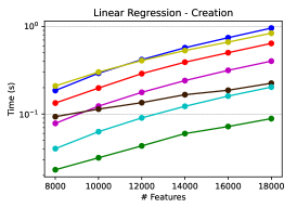
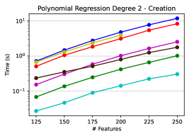
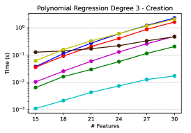
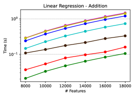
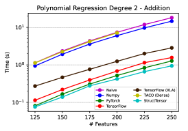
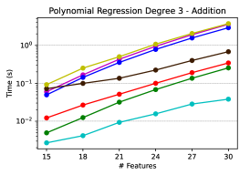
Figure 12. The run time comparison of the covariance matrix creation and addition for linear regression and polynomial regression degree-2 and degree-3. For linear regression dense frameworks show better performance, as the redundancy structure does not pay off. For models with higher redundancy, StructTensor significantly outperforms the competitors thanks to avoiding redundant computation.

7.2. Redundancy Structure

Kernel	Structure of $B$	$B_{U}$ in STUR	TACO (Smart)
TTM	Diagonal (plane)	$(0\leq i<n_{i})*(i=j)*(0\leq l<n_{l})$	$(D,S,D)*(D,D)\rightarrow(D,S,D)$
$A(i,j,k):=$	Fixed $j$	$(0\leq i<n_{i})*(j=J)*(0\leq l<n_{l})$	$(D,S,D)*(D,D)\rightarrow(D,S,D)$
$B(i,j,l)*C(k,l)$	Upper half cube	$(0\leq i<n_{i})*(i\leq j<n_{j})*(0\leq l<n_{l})$	$(D,S,D)*(D,D)\rightarrow(D,S,D)$
THP	Diagonal (plane)	$(0\leq i<n_{i})*(i=j)*(0\leq l<n_{l})$	$(D,S,D)*(D,D,D)\rightarrow(D,S,D)$
$A(i,j,k):=$	Fixed $i$	$(i=I)*(0\leq j<n_{j})*(0\leq l<n_{l})$	$(S,D,D)*(D,D,D)\rightarrow(S,D,D)$
$B(i,j,k)*C(i,j,k)$	Fixed $j$	$(0\leq i<n_{i})*(j=J)*(0\leq l<n_{l})$	$(D,S,D)*(D,D,D)\rightarrow(D,S,D)$
MTTKRP	Fixed $i,j$	$(i=I)*(j=J)*(0\leq l<n_{l})$	$(S,D,D)*(D,D)*(D,S)\rightarrow(S,D)$
$A(i,j):=B(i,k,l)$	Fixed $i$	$(i=I)*(0\leq j<n_{j})*(0\leq l<n_{l})$	$(S,D,D)*(D,D)*(D,D)\rightarrow(S,D)$
$*$ $C(k,j)*D(l,j)$	Fixed $j$	$(0\leq i<n_{i})*(j=J)*(0\leq l<n_{l})$	$(D,D,D)*(D,D)*(D,S)\rightarrow(D,S)$

Table 1. List of tensor kernels for StructTensor evaluation. TACO allows specifying if each dimension is Sparse ($S$) or Dense ($D$). TACO (Smart) specifies the most efficient storage format.

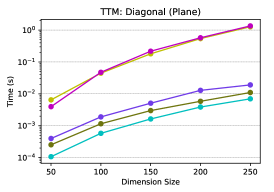
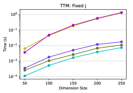
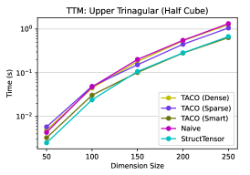
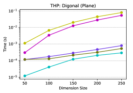
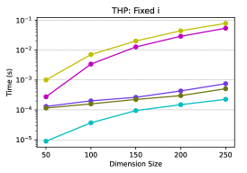
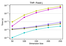
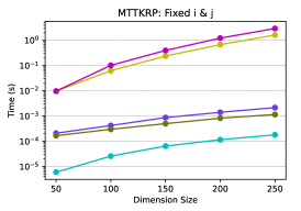
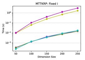
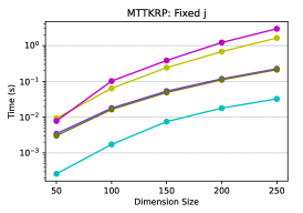
Figure 13. Tensor operation kernels run time comparison using different input and output structures. The naïve version of StructTensor and the dense format of TACO show similar performance. In most cases, the symbolic sparsity employed in StructTensor shows significantly better performance in comparison with the best sparse format used in TACO.

We consider six structured matrix kernels that correspond to the task of creating and addition of covariance matrices for three machine learning models: linear regression, polynomial regression degree-2, and polynomial regression degree-3. As all the matrices only involve redundancy structure, we need to use the dense representation in all systems. As the competitors, we consider TACO (fully dense format), PyTorch, TensorFlow (w/ and w/o the XLA backend), NumPy, and a naïve implementation without leveraging the redundancy structure.

Figure 12 shows the run time comparison. The missing numbers mean that the process was killed due to a segmentation fault. For example, TACO can only handle the polynomial regression degree-2 up to 200 features because it gets killed for more than that. For the kernels with more redundancy (i.e., polynomial regression degree-2 and degree-3), StructTensor outperforms all the competitors from one to two orders of magnitude. However, in linear regression StructTensor only removes half of the computation and because of a lack of data-layout optimizations, loop tiling, and vectorization, performs worse than dense tensor frameworks such as PyTorch and TensorFlow.

7.3. Sparsity Structure

To evaluate the effectiveness of StructTensor for the sparsity structure, we consider three tensor kernels: Tensor Times Matrix (TTM), Tensor Hadamard Product (THP), and Matricized Tensor Times Khatri-Rao Product (MTTKRP). StructTensor is evaluated against TACO with three different formats: fully dense, fully sparse, and smart. In the smart version, we use the most efficient sparse format for TACO based on the sparsity of input and output tensors at each dimension. Table 1 shows the definition of these kernels, the different input structures we considered, their representation in STUR, and the data format at each dimension for TACO (Smart). For StructTensor we consider an additional naïve version that does not leverage the symbolic structure.

Figure 13 represents the run time of each implementation on each kernel. In all kernels i) TACO dense is performing similarly to the naïve implementation, ii) TACO smart is outperforming other data format selections for TACO as expected, and iii) StructTensor outperforms (in 7 out of 9 experiments) or performs on par with TACO smart (despite having a better data layout and generating a more optimized code).

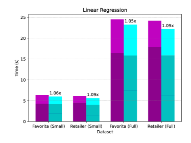
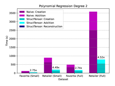
Figure 14. Run time of in-database machine learning over Favorita and Retailer datasets. Here, we compute the covariance matrix of linear and polynomial regression degree-2 over the join of multiple relations.

7.4. End-to-end Experiments

We evaluated StructTensor on an in-database machine learning task. We used StructTensor to create a covariance matrix for linear and polynomial regression degree-2. We consider the following real-world datasets: Retailer (Khamis et al., 2020) with 13 continuous features and Favorita (Favorita, 2017) with 6 continuous features. Both of them have a small (consisting of 25% of the data elements) and full version. StructTensor is compared with a naïve implementation that does not leverage the redundancy structure.

We use the idea of a semi-ring covariance matrix data-structure (Nikolic and Olteanu, 2018; Shaikhha et al., 2022) for both implementations. This data structure pushes joins after aggregates, which heavily improves both memory consumption and run time. In a semi-ring covariance matrix, different degrees of interaction are decoupled and stored separately. This means that for polynomial regression degree-2 (cf. Section 3), we store degree-2 ($M1$), degree-3 ($M2$), and degree-4 ($M3$) interactions separately. Furthermore, degree-3 interactions are calculated twice in both ($\mathbf{f}\otimes vec(\mathbf{f}\otimes\mathbf{f})$) and ($vec(\mathbf{f}\otimes\mathbf{f})\otimes\mathbf{f}$). As the naïve version does not use the structure information, it cannot detect such coarse-grained redundancy information.

Figure 14 represents the run time of StructTensor in comparison with the naïve version. StructTensor produces a structure-aware code that reduces the computations by avoiding redundant computation. Hence, there should be a reconstruction phase that rebuilds the final result and put all elements that have not been computed in their corresponding positions based on the redundancy map. However, the reconstruction time is negligible in comparison with the rest of the computation, as it can be seen in Figure 14.

8. Related Work

Dense Tensor Algebra. Polyhedral frameworks such as isl (Verdoolaege, 2010) and CLooG (Bastoul, 2004) provide efficient loop nest code generation for dense and affine tensor algebra computations. Tensor Comprehension (Vasilache et al., 2018) provides a polyhedral-based DSL supporting generalized Einstein notation that leads to optimized Cuda code generation for dense deep learning computation. TensorFlow (Abadi et al., 2015) provides dense tensor operation for large-scale machine learning applications. All these works provide efficient kernels for dense linear and tensor algebra but for structured tensors, still, they do unnecessary and/or redundant computations.

Sparse Tensor Algebra. The sparse polyhedral framework (Strout et al., 2018) extends the ability of polyhedral compilation to support sparse tensor algebra as well. TACO (Kjolstad et al., 2017) handles sparse and dense computation over tensor algebra. However, unlike StructTensor, none of these work support redundancy-aware computation. Moreover, sparsity is handled in run-time that leads to irregular memory access that are hard to optimize for the compiler (Tang et al., 2020).

Specialized Sparse Linear Algebra. (Augustine et al., 2019) take a different approach by breaking the irregular sparsity patterns into sub-computations with regular structures so they can remove indirect access and provide vectorization to the linear algebra code. EGGS (Tang et al., 2020) further specializes the computation to a sparsity pattern and creates the expression tree of the result by unrolling the entire computing. Performing common-subexpression over the expression tree can partially remove redundancies, but cannot detect symmetric-style patterns. StructTensor infers the redundancy patterns at compilation time to specialize the generated code.

Structured Linear Algebra. LGen (Spampinato and Püschel, 2016) proposes a polyhedral-based technique for code generation of small-scale structured linear algebra. The unique elements are provided in SInfo, and the redundancy information is kept in AInfo. However, it does not support higher-order tensor computations and is limited to fixed-size small-scale matrices. To the best of our knowledge, there is no previous work supporting the structure for higher-order tensors.

Declarative Data Processing Languages. STUR is closely connected to logic languages such as Datalog and Prolog. There are two main differences. First, STUR does not allow recursive definitions. Second, in addition to sets, STUR allows for aggregations over tensors. Dyna (Eisner and Filardo, 2010) extends Datalog by adding to support for maps to real numbers rather than only supporting sets, which are maps to boolean values. FAQ (Khamis et al., 2016) is the main source of inspiration for STUR, which allows for a combination of different semi-rings. The main focus for FAQ has been on efficient algorithms for evaluating sparse tensor contractions appearing in database query engines (Khamis et al., 2020) (e.g., worst-case optimal joins). STUR provides additional constructs for arithmetic operations over the indices and restricting the ranges, which are crucial for efficient structured tensor computations.

Framework	LA	TA	Dense	Sparse	Redundancy	Loop Opts.
Dense TA (TensorFlow)	●	●	●	○	○	●
Dense LA (BLAS)	●	○	●	○	○	●
Sparse TA (TACO, SPLATT)	●	●	●	●	○	●
Sparse LA (MKL, OSKI)	●	○	●	●	○	●
Static Sparse LA (EGGS)	●	○	●	◐ (FS)	◐	●
Structured LA (LGen)	●	○	●	◐ (FS)	●	●
StructTensor	●	●	●	◐ (SY)	●	◐

Table 2. Tensor algebra frameworks comparison. FS: Fixed-size, SY: Symbolic

9. Conclusion & Outlook

In this paper, we presented StructTensor, a compiler for structured tensor algebra. We considered two classes of structures: (1) sparsity patterns, and (2) redundancy structures. We proposed STUR, a unified IR that is expressive enough for tensor computation and captures both forms of structures. We have shown the soundness of transformations and inference rules. Finally, the experimental results show that StructTensor outperforms the state-of-the-art tensor processing libraries.

For the future, we see two clear directions for improvement. First, StructTensor mainly focuses on structure-specific optimizations, and apart from code motion, does not do anything smart for loop optimizations. It would be interesting to use polyhedral-based optimizations (e.g., using CLooG (Bastoul, 2004)) to generate efficient loop nests. Second, for storing tensors, we mainly use $n-d$ arrays, and even the compressed tensors still allocate the memory for the entire uncompressed tensor. Using better layouts can significantly reduce the memory pressure, and would possibly improve data locality.

References

- (1)
- Abadi et al. (2015) Martín Abadi, Ashish Agarwal, Paul Barham, Eugene Brevdo, Zhifeng Chen, Craig Citro, Greg S. Corrado, Andy Davis, Jeffrey Dean, Matthieu Devin, Sanjay Ghemawat, Ian Goodfellow, Andrew Harp, Geoffrey Irving, Michael Isard, Yangqing Jia, Rafal Jozefowicz, Lukasz Kaiser, Manjunath Kudlur, Josh Levenberg, Dandelion Mané, Rajat Monga, Sherry Moore, Derek Murray, Chris Olah, Mike Schuster, Jonathon Shlens, Benoit Steiner, Ilya Sutskever, Kunal Talwar, Paul Tucker, Vincent Vanhoucke, Vijay Vasudevan, Fernanda Viégas, Oriol Vinyals, Pete Warden, Martin Wattenberg, Martin Wicke, Yuan Yu, and Xiaoqiang Zheng. 2015. TensorFlow: Large-Scale Machine Learning on Heterogeneous Systems. https://www.tensorflow.org/ Software available from tensorflow.org.
- Augustine et al. (2019) Travis Augustine, Janarthanan Sarma, Louis-Noël Pouchet, and Gabriel Rodríguez. 2019. Generating piecewise-regular code from irregular structures. In Proceedings of the 40th ACM SIGPLAN Conference on Programming Language Design and Implementation, PLDI 2019, Phoenix, AZ, USA, June 22-26, 2019, Kathryn S. McKinley and Kathleen Fisher (Eds.). ACM, 625–639. https://doi.org/10.1145/3314221.3314615
- Bastoul (2004) Cédric Bastoul. 2004. Code Generation in the Polyhedral Model Is Easier Than You Think. In 13th International Conference on Parallel Architectures and Compilation Techniques (PACT 2004), 29 September - 3 October 2004, Antibes Juan-les-Pins, France. IEEE Computer Society, 7–16. https://doi.org/10.1109/PACT.2004.10018
- Chou et al. (2018) Stephen Chou, Fredrik Kjolstad, and Saman Amarasinghe. 2018. Format abstraction for sparse tensor algebra compilers. Proceedings of the ACM on Programming Languages 2, OOPSLA (2018), 1–30.
- Cichocki et al. (2009) Andrzej Cichocki, Rafal Zdunek, Anh Huy Phan, and Shun-ichi Amari. 2009. Nonnegative matrix and tensor factorizations: applications to exploratory multi-way data analysis and blind source separation. John Wiley & Sons.
- Dongarra et al. (1990) Jack J. Dongarra, Jeremy Du Croz, Sven Hammarling, and Iain S. Duff. 1990. A set of level 3 basic linear algebra subprograms. ACM Trans. Math. Softw. 16, 1 (1990), 1–17. https://doi.org/10.1145/77626.79170
- Eisner and Filardo (2010) Jason Eisner and Nathaniel Wesley Filardo. 2010. Dyna: Extending Datalog for Modern AI. In Datalog Reloaded - First International Workshop, Datalog 2010, Oxford, UK, March 16-19, 2010. Revised Selected Papers (Lecture Notes in Computer Science, Vol. 6702), Oege de Moor, Georg Gottlob, Tim Furche, and Andrew Jon Sellers (Eds.). Springer, 181–220. https://doi.org/10.1007/978-3-642-24206-9_11
- Favorita (2017) Corporacion Favorita. 2017. Corp. Favorita Grocery Sales Forecasting: Can you accurately predict sales for a large grocery chain?
- Gareev et al. (2018) Roman Gareev, Tobias Grosser, and Michael Kruse. 2018. High-Performance Generalized Tensor Operations: A Compiler-Oriented Approach. ACM Trans. Archit. Code Optim. 15, 3 (2018), 34:1–34:27. https://doi.org/10.1145/3235029
- Harris et al. (2020) Charles R. Harris, K. Jarrod Millman, Stéfan J. van der Walt, Ralf Gommers, Pauli Virtanen, David Cournapeau, Eric Wieser, Julian Taylor, Sebastian Berg, Nathaniel J. Smith, Robert Kern, Matti Picus, Stephan Hoyer, Marten H. van Kerkwijk, Matthew Brett, Allan Haldane, Jaime Fernández del Río, Mark Wiebe, Pearu Peterson, Pierre Gérard-Marchant, Kevin Sheppard, Tyler Reddy, Warren Weckesser, Hameer Abbasi, Christoph Gohlke, and Travis E. Oliphant. 2020. Array programming with NumPy. Nature 585, 7825 (Sept. 2020), 357–362. https://doi.org/10.1038/s41586-020-2649-2
- Hegde et al. (2019) Kartik Hegde, Hadi Asghari Moghaddam, Michael Pellauer, Neal Clayton Crago, Aamer Jaleel, Edgar Solomonik, Joel S. Emer, and Christopher W. Fletcher. 2019. ExTensor: An Accelerator for Sparse Tensor Algebra. In Proceedings of the 52nd Annual IEEE/ACM International Symposium on Microarchitecture, MICRO 2019, Columbus, OH, USA, October 12-16, 2019. ACM, 319–333. https://doi.org/10.1145/3352460.3358275
- Hirata (2003) So Hirata. 2003. Tensor Contraction Engine: Abstraction and Automated Parallel Implementation of Configuration-Interaction, Coupled-Cluster, and Many-Body Perturbation Theories. The Journal of Physical Chemistry A 107, 46 (2003), 9887–9897. https://doi.org/10.1021/jp034596z
- Hirata (2006) So Hirata. 2006. Symbolic algebra in quantum chemistry. Theoretical Chemistry Accounts 116, 1 (2006), 2–17.
- Jouppi et al. (2017) Norman P. Jouppi, Cliff Young, Nishant Patil, David A. Patterson, Gaurav Agrawal, Raminder Bajwa, Sarah Bates, Suresh Bhatia, Nan Boden, Al Borchers, Rick Boyle, Pierre-luc Cantin, Clifford Chao, Chris Clark, Jeremy Coriell, Mike Daley, Matt Dau, Jeffrey Dean, Ben Gelb, Tara Vazir Ghaemmaghami, Rajendra Gottipati, William Gulland, Robert Hagmann, C. Richard Ho, Doug Hogberg, John Hu, Robert Hundt, Dan Hurt, Julian Ibarz, Aaron Jaffey, Alek Jaworski, Alexander Kaplan, Harshit Khaitan, Daniel Killebrew, Andy Koch, Naveen Kumar, Steve Lacy, James Laudon, James Law, Diemthu Le, Chris Leary, Zhuyuan Liu, Kyle Lucke, Alan Lundin, Gordon MacKean, Adriana Maggiore, Maire Mahony, Kieran Miller, Rahul Nagarajan, Ravi Narayanaswami, Ray Ni, Kathy Nix, Thomas Norrie, Mark Omernick, Narayana Penukonda, Andy Phelps, Jonathan Ross, Matt Ross, Amir Salek, Emad Samadiani, Chris Severn, Gregory Sizikov, Matthew Snelham, Jed Souter, Dan Steinberg, Andy Swing, Mercedes Tan, Gregory Thorson, Bo Tian, Horia Toma, Erick Tuttle, Vijay Vasudevan, Richard Walter, Walter Wang, Eric Wilcox, and Doe Hyun Yoon. 2017. In-Datacenter Performance Analysis of a Tensor Processing Unit. In Proceedings of the 44th Annual International Symposium on Computer Architecture, ISCA 2017, Toronto, ON, Canada, June 24-28, 2017. ACM, 1–12. https://doi.org/10.1145/3079856.3080246
- Kandemir et al. (1999) Mahmut Kandemir, Alok Choudhary, Nagaraj Shenoy, Prithviraj Banerjee, and J Ramenujarn. 1999. A linear algebra framework for automatic determination of optimal data layouts. IEEE Transactions on Parallel and Distributed Systems 10, 2 (1999), 115–135.
- Khamis et al. (2020) Mahmoud Abo Khamis, Hung Q Ngo, XuanLong Nguyen, Dan Olteanu, and Maximilian Schleich. 2020. Learning models over relational data using sparse tensors and functional dependencies. ACM Transactions on Database Systems (TODS) 45, 2 (2020), 1–66.
- Khamis et al. (2016) Mahmoud Abo Khamis, Hung Q. Ngo, and Atri Rudra. 2016. FAQ: Questions Asked Frequently. In Proceedings of the 35th ACM SIGMOD-SIGACT-SIGAI Symposium on Principles of Database Systems, PODS 2016, San Francisco, CA, USA, June 26 - July 01, 2016, Tova Milo and Wang-Chiew Tan (Eds.). ACM, 13–28. https://doi.org/10.1145/2902251.2902280
- Kjolstad et al. (2017) Fredrik Kjolstad, Shoaib Kamil, Stephen Chou, David Lugato, and Saman Amarasinghe. 2017. The Tensor Algebra Compiler. Proc. ACM Program. Lang. 1, OOPSLA, Article 77 (Oct. 2017), 29 pages. https://doi.org/10.1145/3133901
- Martín-García (2008) José M Martín-García. 2008. xPerm: fast index canonicalization for tensor computer algebra. Computer physics communications 179, 8 (2008), 597–603.
- Nikolic and Olteanu (2018) Milos Nikolic and Dan Olteanu. 2018. Incremental View Maintenance with Triple Lock Factorization Benefits. In Proceedings of the 2018 International Conference on Management of Data (Houston, TX, USA) (SIGMOD ’18). Association for Computing Machinery, New York, NY, USA, 365–380. https://doi.org/10.1145/3183713.3183758
- Paszke et al. (2019) Adam Paszke, Sam Gross, Francisco Massa, Adam Lerer, James Bradbury, Gregory Chanan, Trevor Killeen, Zeming Lin, Natalia Gimelshein, Luca Antiga, Alban Desmaison, Andreas Kopf, Edward Yang, Zachary DeVito, Martin Raison, Alykhan Tejani, Sasank Chilamkurthy, Benoit Steiner, Lu Fang, Junjie Bai, and Soumith Chintala. 2019. PyTorch: An Imperative Style, High-Performance Deep Learning Library. In Advances in Neural Information Processing Systems 32. Curran Associates, Inc., 8024–8035. http://papers.neurips.cc/paper/9015-pytorch-an-imperative-style-high-performance-deep-learning-library.pdf
- Ran et al. (2020) Shi-Ju Ran, Emanuele Tirrito, Cheng Peng, Xi Chen, Luca Tagliacozzo, Gang Su, and Maciej Lewenstein. 2020. Tensor network contractions: methods and applications to quantum many-body systems. Springer Nature.
- Schleich et al. (2022) Maximilian Schleich, Amir Shaikhha, and Dan Suciu. 2022. Optimizing Tensor Programs on Flexible Storage. arXiv preprint arXiv:2210.06267 (2022).
- Shaikhha et al. (2022) Amir Shaikhha, Mathieu Huot, Jaclyn Smith, and Dan Olteanu. 2022. Functional collection programming with semi-ring dictionaries. Proceedings of the ACM on Programming Languages 6, OOPSLA1 (2022), 1–33.
- Smith and Gray (2018) Daniel G. A. Smith and Johnnie Gray. 2018. opt_einsum - A Python package for optimizing contraction order for einsum-like expressions. J. Open Source Softw. 3, 26 (2018), 753. https://doi.org/10.21105/joss.00753
- Spampinato and Püschel (2016) Daniele G. Spampinato and Markus Püschel. 2016. A basic linear algebra compiler for structured matrices. In Proceedings of the 2016 International Symposium on Code Generation and Optimization, CGO 2016, Barcelona, Spain, March 12-18, 2016, Björn Franke, Youfeng Wu, and Fabrice Rastello (Eds.). ACM, 117–127. https://doi.org/10.1145/2854038.2854060
- Strout et al. (2018) Michelle Mills Strout, Mary Hall, and Catherine Olschanowsky. 2018. The sparse polyhedral framework: Composing compiler-generated inspector-executor code. Proc. IEEE 106, 11 (2018), 1921–1934.
- Tang et al. (2020) Xuan Tang, Teseo Schneider, Shoaib Kamil, Aurojit Panda, Jinyang Li, and Daniele Panozzo. 2020. EGGS: Sparsity-Specific Code Generation. Comput. Graph. Forum 39, 5 (2020), 209–219. https://doi.org/10.1111/cgf.14080
- Titov et al. (2013) Alexey V Titov, Ivan S Ufimtsev, Nathan Luehr, and Todd J Martinez. 2013. Generating efficient quantum chemistry codes for novel architectures. Journal of chemical theory and computation 9, 1 (2013), 213–221.
- Vasilache et al. (2018) Nicolas Vasilache, Oleksandr Zinenko, Theodoros Theodoridis, Priya Goyal, Zachary DeVito, William S Moses, Sven Verdoolaege, Andrew Adams, and Albert Cohen. 2018. Tensor comprehensions: Framework-agnostic high-performance machine learning abstractions. arXiv preprint arXiv:1802.04730 (2018).
- Verdoolaege (2010) Sven Verdoolaege. 2010. isl: An Integer Set Library for the Polyhedral Model. In Mathematical Software (ICMS’10) (LNCS 6327), Komei Fukuda, Joris Hoeven, Michael Joswig, and Nobuki Takayama (Eds.). Springer-Verlag, 299–302.