Strong cosmological constraints on the neutrino magnetic moment

Abstract

A sizable magnetic moment for neutrinos would be evidence of exotic physics. In the early Universe, left-handed neutrinos with a magnetic moment would interact with electromagnetic fields in the primordial plasma, flipping their helicity and producing a population of right-handed (RH) neutrinos. In this work, we present a new calculation of the production rate of RH neutrinos in a multi-component primordial plasma and quantify their contribution to the total energy density of relativistic species at early times, stressing the implications of the dependence on the initial time for production. Our results improve the previous cosmological limits by almost two orders of magnitudes. Prospects for upcoming cosmological experiments are also discussed.

I Introduction

The existence of a sizable neutrino magnetic moment ($\mu$) is a fascinating possibility, which has produced a vivid interest from both the experimental and phenomenological side in the recent years. Historically, the hypothesis of a neutrino magnetic moment is almost as long as the history of neutrinos themselves. The first experimental constraint goes back to the very neutrino discovery experiment by Cowan and Reines [1]. Analyzing electron recoil spectra in (anti)-neutrino electron scattering, the authors derived the bound $\mu\lesssim 10^{-9}\,\mu_{B}$, where $\mu_{B}=e/2m_{e}$ denotes the Bohr magneton. Later searches gave considerably stronger constraints [2, 3, 4, 5, 6]. The current experimental sensitivity slightly below $10^{-11}$ $\mu_{B}$.

Although massive neutrinos, with a Dirac mass, are expected to have a magnetic moment [7], this is predicted to be quite small, $\mu\approx 3\times 10^{-19}\times(m_{\nu}/1\,{\rm eV})\,\mu_{B}$. Thus, a sizable magnetic moment would be evidence of exotic physics. Furthermore, even though several extensions of the standard model predict a larger neutrino magnetic moment, the predictions change substantially for Dirac and Majorana neutrinos, with the latter allowed more naturally to have a large $\mu$ [8, 9, 10, 11]. Hence, a discovery of a sufficiently large magnetic moment would also shed light on the nature of the neutrino field.

A non-vanishing neutrino magnetic moment would have profound astrophysical and cosmological consequences. Stellar evolution provides some of the strongest bounds on $\mu$. The resulting tree-level neutrino-photon interaction contributes substantially to several cooling mechanisms in stars (see, e.g., Ref. [12] for a comprehensive discussion), most notably to the plasmon decay $\gamma\to\bar{\nu}\nu$. A recent analysis of the cooling of red giant stars [13] provided the constraint $\mu\lesssim 1.2\times 10^{-12}\mu_{B}$, about a factor of 5 below the current experimental sensitivity.

Furthermore, for Dirac neutrinos, a non-vanishing magnetic moment would induce the production of right-handed (RH) neutrinos via spin-flip of left-handed (LH) neutrinos in an external electromagnetic field. For a supernova, where LH neutrinos are trapped and RH neutrinos are not, this would imply a very efficient energy loss mechanism [14, 15, 16]. Spin-flip processes may also play a significant role in the early Universe, given the large number of charged particles generating electromagnetic fields required for this process to take place. The production of RH neutrinos in this case would affect the predictions of the light-elements abundance because of the increased number of relativistic degrees of freedom $N_{\mathrm{eff}}$ [17, 18, 19, 20]. In the past, the above observables were used to derive the constraint $\mu\lesssim 6.2\times 10^{-11}\mu_{B}$ [21], a result considerably less stringent than the current astrophysical limits. The analysis of Ref. [21], however, did not account for the spin flip processes in the electromagnetic field generated by charged particles other than electrons and positrons. In the early universe, especially above the phase transition of the Quantum Chromodynamics (QCD), we expect a large number of charged particles and thus more efficient spin-flip processes. Current and upcoming cosmological surveys severely constrain the number of relativistic degrees of freedom $N_{\mathrm{eff}}$. These constraints can be directly translated into tighter bounds on $\mu$. This encouraged us to revise the analysis and to update the results, accounting for all the relevant contributions in the early universe.

In this work we present a novel calculation of RH neutrino production in the early Universe to accommodate an arbitrary number of charges with different masses. The calculation is performed using thermal field theory methods and presented in sec. II. Then, in sec. III, we derive cosmological implications for neutrinos with a magnetic moment. As we shall see in sec. IV, the requirement of not exceeding the number of effective relativistic species allowed by cosmological observations would result in a strong constraint on the neutrino magnetic moment.

II RH neutrino production rate

Neutrinos with a magnetic moment interact with the surrounding plasma through current-current interactions with the electromagnetic fields generated by charged particles. Information about the medium and its electromagnetic fluctuations are encoded in the imaginary part of the photon polarization tensor $\Pi_{\mu\nu}$. Indeed, the one-loop polarization tensor is obtained by summing over loops with all the charged particles in a plasma and its imaginary part is a measure of the electromagnetic plasma fluctuations. Ref. [21] calculated the RH neutrinos production rate in a hot plasma using the Thermal Field Theory approach. Explicitly, the net production rate of RH neutrinos is

$$\begin{split}\Gamma=&\frac{\mu^{2}}{2\pi}\int_{0}^{\infty}dk\,k\int_{-\infty}^{\infty}dk_{0}\theta\left(-K^{2}(K^{2}+4pk_{0}+4p^{2})\right)\\ &\epsilon(k_{0})\frac{K^{4}}{k^{2}}\Bigg{[}\frac{\epsilon(k_{0})}{e^{\frac{|p_{0}+k_{0}|}{T}}+1}+\frac{\epsilon(p_{0}+k_{0})}{e^{\frac{|k_{0}|}{T}}+1}+\\ &+\epsilon(p_{0}+k_{0})\theta(-k_{0})-\epsilon(k_{0})\theta(-k_{0}-p_{0})\Bigg{]}\\ &\left[\left(1+\frac{k_{0}}{p}+\frac{K^{2}}{4p^{2}}\right)\mathcal{A}_{T}(K)-\left(1+\frac{k_{0}}{2p}\right)^{2}\mathcal{A}_{L}(K)\right]\,,\end{split}$$ (1)

where $(p_{0},p)$ is the neutrino four-momentum, $K=(k_{0},k)$ is the photon four-momentum, $T$ is the temperature of the thermal bath, $\theta$ is the Heaviside theta function, $\epsilon$ is the sign function, and the sources of electromagnetic fields are encoded in the photon spectral functions $\mathcal{A}_{T,L}$, defined as

$$\mathcal{A}_{T,L}(K)=-\frac{1}{\pi}\frac{{\rm Im}\Pi_{T,L}}{|K^{2}-{\rm Re}\Pi_{T,L}|^{2}+|{\rm Im}\Pi_{T,L}|^{2}}\,,$$ (2)

in terms of the transverse $\Pi_{T}$ and longitudinal $\Pi_{L}$ components of the photon polarization tensor. Explicitly, in a single component plasma with a fermion of mass $m_{f}$ and charge $e_{f}$ the photon polarization tensor is given by [22]

$$\begin{split}\Pi_{L}(m_{f},e_{f})&=-\frac{K^{2}}{k^{2}}u^{\mu}u^{\nu}\Pi_{\mu\nu}\,,\\ \Pi_{T}(m_{f},e_{f})&=-\frac{1}{2}\Pi_{L}+\frac{1}{2}g^{\mu\nu}\Pi_{\mu\nu}\,,\\ \end{split}$$ (3)

where $g^{\mu\nu}$ is the metric tensor, $u^{\mu}$ is the plasma four-velocity, which in the rest frame reduces to $u^{\mu}=(1,0,0,0)$, while

$$\begin{split}&u^{\mu}u^{\nu}\Pi_{\mu\nu}=e_{f}^{2}\int\frac{dq\,q^{2}}{2E_{q}\pi^{2}}\frac{1}{e^{E_{q}/T}+1}\bigg{[}2+\\ &-\frac{(2E_{q}+\omega)^{2}-k^{2}}{4qk}\ln\left(\frac{\omega^{2}-k^{2}+2(E_{q}\omega+qk)}{\omega^{2}-k^{2}+2(E_{q}\omega-qk)}\right)+\\ &+\frac{(2E_{q}-\omega)^{2}-k^{2}}{4qk}\ln\left(\frac{\omega^{2}-k^{2}-2(E_{q}\omega+qk)}{\omega^{2}-k^{2}-2(E_{q}\omega-qk)}\right)\bigg{]}\,,\end{split}$$ (4)

and

$$\begin{split}&g^{\mu\nu}\Pi_{\mu\nu}=2e_{f}^{2}\int\frac{dq\,q^{2}}{2E_{q}\pi^{2}}\frac{1}{e^{E_{q}/T}+1}\bigg{[}2+\\ &+\frac{\omega^{2}-k^{2}+2m_{f}^{2}}{4qk}\ln\left(\frac{\omega^{2}-k^{2}+2(E_{q}\omega-qk)}{\omega^{2}-k^{2}+2(E_{q}\omega+qk)}\right)+\\ &-\frac{\omega^{2}-k^{2}+2m_{f}^{2}}{4qk}\ln\left(\frac{\omega^{2}-k^{2}-2(E_{q}\omega-qk)}{\omega^{2}-k^{2}-2(E_{q}\omega+qk)}\right)\bigg{]}\,,\\ \end{split}$$ (5)

with $E_{q}=\sqrt{q^{2}+m_{f}^{2}}$ the energy of the fermion in the loop. In a multi-component plasma, the full polarization tensor is obtained by summing Eqs. (4)-(LABEL:eq:gpi) over all the species $f$

$$\Pi_{T,L}=\sum_{f}\Pi_{T,L}(m_{f},e_{f})\,.$$ (6)

Our result is in agreement with Ref. [21] in the limiting case of massless electrons. However, our approach allows us to extend the evaluation of the production rate to the more realistic case of a multi-component plasma, including both leptons and quarks, as the one found in the early Universe at temperatures larger than the QCD critical scale.

Notice that the low-momentum part of the rate in Eq. (1) features an infrared divergence which has to be regularized. In Ref. [21] the regularization is provided by the thermal photon mass, $m_{\gamma}=e\,T/3$, which determines a low-momentum cut-off. Here, we propose a different regularization method, based on the following observation. When the photon approaches the on-shell condition, the imaginary part of the polarization tensor vanishes, ${\rm Im}\Pi_{T,L}\to 0$, and Eq. (2) reduces to a Dirac delta function $\delta(K^{2}-{\rm Re}\Pi_{T,L})$. Therefore, the divergence can be regularized by replacing the integration over the photon energy with the only contribution coming from the on-shell photon. We underline that this treatment affects only slightly our results since the observables are obtained by integrating over $(p/T)^{3}\,\Gamma(p/T)$ [see Eq. (10) in the next Section]. Thus, the low-momentum contribution is strongly suppressed and different regularization schemes give comparable results.

In the upper panel of Fig. 1, we show the production rate $\Gamma$ for RH neutrinos as a function of $p/T$. For small values of the momentum, the rate increases due to aforementioned resonances, in which on-shell longitudinal or transverse photon excitations are exchanged. The rate increases with the number of charged species in the plasma which, at any given time, contribute to the effective number of entropy degrees of freedom, $g_{*,s}(T)$. As shown in the upper panel of Fig. 1, $\alpha^{-1}\mu^{-2}T^{-3}\Gamma(p,T)/\sqrt{g_{*,s}(T)}$ is approximately constant within a $\sim O(1)$ factor for $T\gtrsim 10\,\operatorname{MeV}$. After averaging the rates over a thermal neutrino distribution, we find that at $T=100$ GeV the rate is

$$\langle\Gamma\rangle=6.04\,\alpha\,\mu^{2}\,T^{3}\,.$$ (7)

For $T=10$ MeV, where the thermal bath includes only electrons, we find $\langle\Gamma\rangle=1.91\,\alpha\,\mu^{2}\,T^{3}\,$, to be compared with $\langle\Gamma\rangle=1.81\,\alpha\mu^{2}\,T^{3}$ in Ref. [21]. The full shape of $\langle\Gamma\rangle/(\alpha\mu^{2}\,T^{3})$ is shown in the lower panel of Fig. 1, where the series of drops below $T\approx 100\,\mathrm{GeV}$ are due to changes in $g_{*,s}(T)$. Our calculation of the rate smoothly interpolates between different temperatures by explicitly taking into account the mass of the charged particles. Indeed, the spin-flip is efficient in the electromagnetic field of relativistic particles and as the temperature decreases, less targets are available.

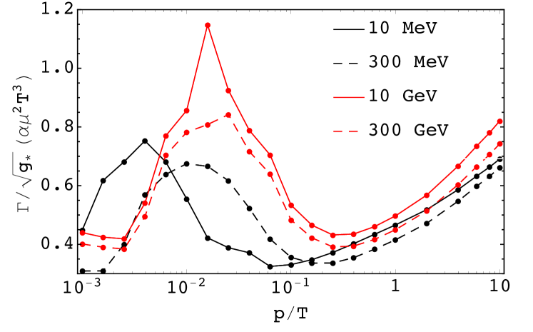
Figure 1: Upper panel: production rate $\Gamma$ for RH neutrinos as a function of the neutrino momentum in terms of $p/T$, for different values of temperature: $10\,\operatorname{MeV}$ (solid black line), $300\,\operatorname{MeV}$ (dashed black line), $10\,\operatorname{GeV}$ (solid red line) and $300\,\operatorname{GeV}$ (solid red line). The lines are a linear interpolation between the values of $p/T$ at which the rate is computed, marked by circles. The rate is normalized to $\alpha\mu^{2}\sqrt{g_{*,s}(T)}T^{3}$ and after this rescaling the temperature dependence of the rate is mild, especially for $p/T>1$.
Lower panel: thermally-averaged production rate as a function of temperature. The solid curves show a linear interpolation between the values of $T$ at which the rate is computed, marked by circles.

III Cosmological implications

The phase-space distribution function for RH neutrinos, $f^{R}(t,q)$ of comoving momentum $q=ap$, with $a$ the cosmological scale factor, evolves according to the following Boltzmann equation [21]:

$$\partial_{t}\left(f^{R}-f^{\mathrm{eq}}\right)=-\Gamma\left(f^{R}-f^{\mathrm{eq}}\right),$$ (8)

where $f^{\mathrm{eq}}(q)$ is the time-independent equilibrium distribution function. As long as $f^{\mathrm{eq}}$ is the true equilibrium distribution, we may recast Eq. (8) as $\partial_{t}f^{R}=-\Gamma(p)\left(f^{R}-f^{\mathrm{eq}}\right)$. We now take $f^{\mathrm{eq}}$ to be the distribution function of the left-handed neutrinos $f_{\nu}$, which are kept in thermal equilibrium with the primordial plasma at temperature $T$ by the weak interactions

$$f^{\mathrm{eq}}=f_{\nu}=\frac{1}{\exp{\left(\frac{q}{aT}\right)}+1}\,.$$ (9)

Notice that, since the plasma temperature scales as $aT\propto g_{*,s}^{-1/3}$ , $f_{\nu}$ is not, in general, time-independent. Thus, identifying $f_{\nu}$ with the equilibrium distribution is strictly valid only if the effective number of entropy degrees of freedom $g_{*,s}$ is constant. Nevertheless, the assumption in Eq. (9) reproduces the expected behavior of $f_{R}$ in the limits that are most relevant for our analysis. To better clarify this issue, it is convenient to recast Eq. (8) as $\partial_{x}f^{R}=-\Gamma/H\left(f^{R}-f_{\nu}\right)$, where $x\equiv\log\,a$, $f^{\mathrm{eq}}=f_{\nu}$ and $H$ is the Hubble parameter. Obviously, for $\Gamma/H=0$, we find that $\partial_{x}f_{R}=0$, as expected since in this case right handed neutrinos are always decoupled. In the opposite limit, $\Gamma/H\gg 1$, we find $f_{R}\approx f_{\nu}$. This is also the expected result, since in this case the RH neutrino population rapidly catches up with the active neutrinos and share the same distribution function. Thus, our assumption in Eq. (9) reproduces well the expected evolution of the RH neutrinos abundances except in the rare event in which $\Gamma/H\approx 1$ at a time when $g_{*,s}$ is changing. We expect that neglecting this effect does not affect significantly our results and defer a more complete numerical treatment of the right-left neutrino evolution to a future work.

The evolution equation is solved for $f^{R}(x)$ over a grid of values of the comoving momentum, together with the initial condition $f^{R}_{in}=0$, i.e., no initial population of RH neutrinos. The initial time of integration, corresponding to a temperature $T_{\mathrm{in}}$, can be chosen arbitrarily and, as we shall see, possibly affects the outcome of the computation. We always integrate the Boltzmann equation down to $T_{\mathrm{fin}}=10\,\operatorname{MeV}$. At lower temperatures, the spin-flip rate becomes rapidly negligible, and no significant production of RH neutrinos takes place. The formalism laid down in Sec. II allows us to coherently compute the production rate $\Gamma$ while taking into account the contribution from the correct number of charged species at any given time back to early epochs.

The ratio $\left\langle\Gamma\right\rangle/H\propto\mu^{2}T$ in the radiation-dominated era, and for constant $g_{*,s}$. The production of RH neutrinos will then be dominated by the high-temperature regime, and our results might depend on the initial time chosen for the integration. In fact, defining the decoupling temperature $T_{d}$ through $\left\langle\Gamma\right\rangle/H|_{T_{d}}=1$, RH neutrinos will quickly thermalize at around the initial time if $T_{\mathrm{in}}\gg T_{d}$, and their final abundance will be independent of $T_{\mathrm{in}}$. The abundance relative to active neutrinos will thus only depend on entropy injections in the plasma happening at $T<T_{d}$. On the other hand, in the regime $T_{\mathrm{in}}\lesssim T_{d}$ the abundance of RH neutrinos will depend on $T_{\mathrm{in}}$, since their production will be happening out-of-equilibrium, in a “freeze-in” kind of process, and $T_{\mathrm{in}}$ will set the time interval during which RH neutrinos can be efficiently produced.

The extra contribution $\Delta N_{\mathrm{eff}}$ to the effective number of relativistic degrees of freedom $N_{\mathrm{eff}}$ due to the population of a single species of RH neutrinos at a given time is obtained by opportunely integrating $f^{R}$ over the phase space:

$$\Delta N_{\mathrm{eff}}(T)=\frac{\int\mathrm{d}p\,p^{3}f^{R}(p,T)}{\int\mathrm{d}p\,p^{3}f_{\nu}(p,T)}\,.$$ (10)

In Fig. 2, we show the evolution of $\Delta N_{\mathrm{eff}}(T)$ for different values of $\mu$ taking the initial temperature to be $T_{\mathrm{in}}=100\,\mathrm{GeV}$. On each curve, we mark with a small circle the time of decoupling corresponding to that value of $\mu$. There are no circles on the curves for $\mu=10^{-12}$ and $10^{-9}\mu_{B}$, as those would lie outside the temperature range shown in the plot (at higher and lower temperatures, respectively). Note how, for the largest values of $\mu$ in the plot, the extra contribution $\Delta N_{\mathrm{eff}}$ quickly reaches a saturation limit corresponding to a thermal abundance at the photon temperature, with the transition epoch from negligible contribution to thermal abundance weakly depending on $\mu$. The drop in $\Delta N_{\mathrm{eff}}(T)$ at later times is due to entropy injection in the plasma happening after the decoupling of RH neutrinos (particularly evident is the drop at the QCD phase transition, $T\approx 150\,\operatorname{MeV}$). In this regime, the final abundance is thus basically set by the decoupling temperature.

For lower values of $\mu$ ($\mu/\mu_{B}\lesssim 10^{-11}$ for $T_{\mathrm{in}}=100\,\operatorname{GeV}$), RH neutrinos do not have enough time to thermalize. In this regime $\Delta N_{\mathrm{eff}}$ decreases with decreasing $\mu$ due both to entropy production and a smaller RH population. As expected, $\Delta N_{\mathrm{eff}}$ becomes negligibly small for vanishing $\mu$. In the plot we also include the case for $\mu/\mu_{B}=10^{-11}$ and $T_{\mathrm{in}}=1\,\mathrm{GeV}$, shown as a dashed red line. The lower initial temperature implies that, despite the rapid initial growth, $\Delta N_{\mathrm{eff}}$ remains significantly smaller than the corresponding contribution obtained for the same $\mu$ value but $T_{\mathrm{in}}=100\,\mathrm{GeV}$ (solid red line).

In the following, we take the “late-time” value of $\Delta N_{\mathrm{eff}}(T)$ as the one relevant for cosmological observations. $\Delta N_{\mathrm{eff}}(T)$ is constant for $T\lesssim 10\,\operatorname{MeV}$ since after that time no significant production of RH neutrinos takes place after that time, as commented above, and the comoving density of active neutrinos does not change either in the limit of instantaneous decoupling. We then use $\Delta N_{\mathrm{eff}}(T=10\,\operatorname{MeV})$ as the late-time value of $\Delta N_{\mathrm{eff}}$.

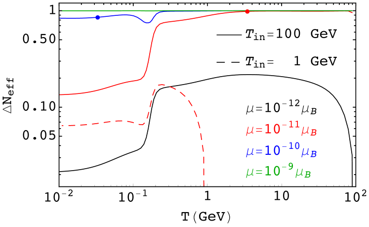
Figure 2: Evolution of $\Delta N_{\mathrm{eff}}$ due to the population of a single species of RH neutrinos induced by spin-flip interactions with active neutrinos through $\mu$, as per Eq. (10). The solid lines are obtained for $T_{\mathrm{in}}=100\,\mathrm{GeV}$ and different values of $\mu$. For comparison, the dashed line is obtained for $\mu/\mu_{B}=10^{-11}$ and $T_{\mathrm{in}}=1\,\mathrm{GeV}$. The dots mark the values of the decopuling temperature $T_{d}$. The dots for $\mu=10^{-12}$ and $10^{-9}\mu_{B}$ lie outside the temperature range shown in the plot (at higher and lower temperatures, respectively)

IV Discussion and conclusions

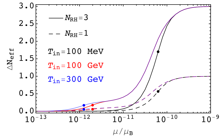
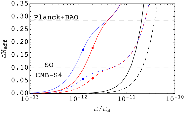
Figure 3: Upper panel: $\Delta N_{\mathrm{eff}}$ due to the population of three (solid) or one (dashed) species of RH neutrinos as function of $\mu$ for different initial temperatures: $T_{\rm in}=100$ MeV (black lines), $T_{\rm in}=100$ GeV (red lines) and $T_{\rm in}=300$ GeV (blue lines). Lower panel: the same as the upper panel, zoomed in the region where $\Delta\,N_{\rm eff}<0.35$. The horizontal dashed lines indicate the current bounds (Planck+BAO) and the sensitivity of future experiments (SO and CMB-S4) (95% credible intervals in both cases). The dots mark the values of $\mu$ giving $\left\langle\Gamma\right\rangle/H=1$ at $T=T_{\mathrm{in}}$.

Our main result is shown in Fig. 3, where we report the late-time contribution $\Delta N_{\mathrm{eff}}$ as a function of $\mu$ for different initial temperatures, in the case of one or three species of RH neutrinos. As expected, in the limit of very large $\mu$, the RH population remains coupled to the active neutrino species until late times, hence providing a large contribution to $N_{\mathrm{eff}}$. For lower values of the $\mu$, RH neutrinos would still be in thermal equilibrium with the plasma at early times, but the decoupling would happen earlier. In this scenario, RH neutrinos are efficiently diluted by entropy production and their contribution to $N_{\mathrm{eff}}$ is smaller. In the limit of vanishing $\mu$, we enter the regime in which RH neutrinos are never coupled to the active species. In this case, a residual non-thermal population of RH neutrinos can develop and contribute very feebly, yet non-vanishingly, to $N_{\mathrm{eff}}$. As we shall see, this has important consequences when confronted with observations. The horizontal dashed lines in the bottom panel correspond to the (95% credible interval) bounds on $\Delta N_{\mathrm{eff}}$ from a combination of current cosmological data (observations of CMB anisotropies from Planck and of baryon acoustic oscillations from a combination of large-scale-structure surveys, see Ref. [29]) and to the expected $2\sigma$ sensitivity on $\Delta N_{\mathrm{eff}}$ from future CMB surveys (the Simons Observatory, SO, [30] and CMB-S4 [31]). Taking $T_{\mathrm{in}}=100\,\mathrm{GeV}$ as our benchmark, the current $N_{\mathrm{eff}}$ measurement from Planck+BAO, $N_{\mathrm{eff}}=2.99^{+0.34}_{-0.33}$ (95% credible interval) implies:

$$\mu<4.6\times 10^{-12}\mu_{B}\quad(\textrm{Planck+BAO})$$ (11)

Future cosmological data will be able to test $\mu$ values as low as $\mu=1.3\times 10^{-12}\mu_{B}$ (SO) and $\mu=0.96\times 10^{-12}\mu_{B}$ (CMB-S4).

In the plot we also mark with small circles the values of $\mu_{B}$ that yield $\left\langle\Gamma\right\rangle/H=1$ at the initial temperature. The part of each curve on the right of the circle corresponds to the thermal regime, $\left\langle\Gamma\right\rangle/H>1$ at $T_{\mathrm{in}}$. Note that all curves overlap to the right of the respective circle, signaling that the final abundance of RH neutrinos is independent of the initial temperature when $\mu$ is such that $T_{d}\ll T_{\mathrm{in}}$. Conversely, the region on the left of the circles traces the freeze-in regime, $\left\langle\Gamma\right\rangle/H<1$ at $T_{\mathrm{in}}$. Thus, while the current constraints from Planck+BAO are probing the thermal regime, next-generation experiments will go deep in the freeze-in regime, at least in the case of three RH neutrino families. We in fact stress that, given the dependence of $\Delta N_{\mathrm{eff}}$ on $\mu$, a non-detection of $\Delta N_{\mathrm{eff}}$ from future cosmological surveys cannot be interpreted as the absence of a residual population of RH neutrinos. Indeed, if neutrinos are Dirac particles and $\mu\neq 0$, such a population should exist, albeit extremely diluted due to the very small value of the production rate $\Gamma$.

The upper bound on $\mu$ from current data corresponds to $T_{d}<100\,\operatorname{GeV}$ and to the presence of a thermal population of RH neutrinos. In fact $\mu=4\times 10^{-12}\mu_{B}$ gives $T_{d}\simeq 20\,\operatorname{GeV}$. In this regime, the final abundance would not depend on $T_{\mathrm{in}}$, but rather on the value of $g_{*s}$ at decoupling, and increasing $T_{\mathrm{in}}$ would not change the abundance. One would thus find the same bound on $\mu$ from Planck+BAO for $T_{\mathrm{in}}>100\,\operatorname{GeV}$. This can be noticed in the top panel of Fig. 3, where the curves for $T_{\mathrm{in}}=100$ and $T_{\mathrm{in}}=300\,\operatorname{GeV}$ overlap to the right of the circle and, in particular, at the point where they intersect the Planck+BAO line (bottom panel), so that they yield the same bound on $\mu$. Decreasing $T_{\mathrm{in}}$ would instead start changing the abundance as soon as $T_{\mathrm{in}}\leq T_{d}$. In this case, the same value of $\mu$ that led instead to thermal abundance for $T_{\mathrm{in}}\geq T_{d}$ corresponds to a freeze-in scenario, with lower-than-thermal abundance. In this regime, current data can accommodate larger values of $\mu$. This can again be seen by comparing the curves for $100\,\operatorname{GeV}$ and $100\,\operatorname{MeV}$ in Fig. 3, with the latter providing a weaker bound on $\mu$ than the former.

The sensitivity of future CMB experiments will instead allow to probe the freeze-in regime at $T_{\mathrm{in}}=100\,\operatorname{GeV}$. A magnetic moment $\mu=10^{-12}\,\mu_{B}$, yielding $\Delta N_{\mathrm{eff}}=0.06$ for $T_{\mathrm{in}}=100\,\operatorname{GeV}$, corresponds to a decoupling temperature $T_{d}\simeq 300\,\operatorname{GeV}$. For constant $g_{*s}$, the freeze-in abundance is proportional to $\mu^{2}T_{\mathrm{in}}$. The upper bound on $\mu$ will then become tighter for $T_{\mathrm{in}}>100\,\operatorname{GeV}$, scaling as $1/\sqrt{T_{\mathrm{in}}}$. In fact, when deriving constraints on $\mu$ using the rates computed at $10^{3}\,\operatorname{GeV}$, we find $\mu<3.4\times 10^{-13}$ for CMB-S4, in line with the expected $\sqrt{10}$ improvement. Note that the fact that the decoupling temperature also scales as $\mu^{2}$ (again for constant $g_{*s}$) ensures that the rescaled constraint will still correspond to the freeze-in regime.

As we anticipated in sec. III, the choice of $T_{\mathrm{in}}$ is somehow arbitrary. In principle, the initial temperature can be taken as large as the highest reheating temperature currently allowed by the non-observation of primordial $B$-modes in the cosmic microwave background. The combination of Planck 2018 and BICEP-Keck 2015 data gives an upper bound of $(1.6\times 10^{16}\,\operatorname{GeV})^{4}$ for the energy density $V$ at inflation [32]. Assuming a perfectly efficient reheating, we could take $T_{\mathrm{in}}\sim V^{1/4}$. This could give extremely tight bounds on $\mu$. An extrapolation to such high energies might however be unreliable, as some of the approximations made could fail. For example, several theories beyond the standard model predict new degrees of freedom that could contribute to $g_{*s}$ at such high temperatures.

A careful extension of the formalism laid down in this work is therefore required to project the sensitivity on $\mu$ in the regime $T_{\mathrm{in}}\gg 100\,\mathrm{GeV}$. Furthermore, it cannot be excluded that the Universe underwent other reheating episodes in addition to the one associated to the end of inflation. In fact, the latest of such reheating events can happen at a temperature $T_{\mathrm{RH}}$ as low as a few MeV without contradicting available observations [33]. In such a low-reheating scenario, $T_{\mathrm{in}}\simeq T_{\mathrm{RH}}$. The limits presented above would be relaxed if $T_{\mathrm{RH}}<100\,\operatorname{GeV}$, as it can be seen from Fig. 3. For example, for $T_{\mathrm{in}}=100\,\operatorname{MeV}$, the current limit from Planck+BAO would be relaxed to $\mu<2.1\times 10^{-11}\,\mu_{B}$, while the CMB-S4 sensitivity would be degraded to $9.2\times 10^{-12}\mu_{B}$.

To summarise, the choice of $T_{\mathrm{in}}=100\,\operatorname{GeV}$ as a benchmark can be regarded as cautious: going much above $T_{\mathrm{in}}=100\,\operatorname{GeV}$ would require assumptions on the validity of the standard model of particle physics at very high temperatures; going below $T_{\mathrm{in}}=100\,\operatorname{GeV}$ would require to assume significant deviations from the standard model of cosmology.

Note added

A few days before our manuscript was completed, the work in Ref. [34], which partially overlaps with ours, appeared. The authors of Ref. [34] evaluated the RH neutrino production rate using a different approach, which lead to a rate $\sim 50\%$ smaller than the one presented here. The qualitative conclusions of our work would be unaffected by this change and we plan to investigate in details the differences between the two approaches. At any rate, it is important to remark that our approach contains significant novelties and sensibly differs from the analysis in Ref. [34]. First, we generalize the thermal field theory formalism to account for the mass of the fermions in the multi-component plasma. This allows us to correctly follow the interaction of neutrinos with a magnetic moment with the plasma up to very early epochs. Second, we evolve the relevant Boltzmann equation to obtain the distribution function of RH neutrinos and subsequently the contribution of the latter to $N_{\mathrm{eff}}$. In doing so, we do not need to assume that RH neutrinos are in thermal equilibrium to begin with. This assumption is relevant, since it explains the different result we obtain for $N_{\mathrm{eff}}$ in the limit of negligibly small $\mu$. In Ref. [34], there is a non-vanishing lower bound on the predicted contribution to $N_{\mathrm{eff}}$ from the maximum allowed dilution factor from $g_{*,s}$. In our case, a very small $\mu$ could lead to the RH neutrinos never reaching equilibrium with the active population. The resulting (non-thermal) contribution to $N_{\mathrm{eff}}$ is vanishingly small, yet non-zero. Thus, even in the case of non-thermalized RH neutrinos, a non-detection of $\Delta N_{\mathrm{eff}}$ above the threshold of future CMB surveys cannot be interpreted in terms of a vanishing $\mu$.

References

- [1] C. L. Cowan and F. Reines, Neutrino magnetic moment upper limit, Phys. Rev. 107 (1957) 528.
- [2] F. Reines, H. S. Gurr and H. W. Sobel, Detection of anti-electron-neutrino e Scattering, Phys. Rev. Lett. 37 (1976) 315.
- [3] TEXONO Collaboration, H. B. Li et al., Limit on the electron neutrino magnetic moment from the Kuo-Sheng reactor neutrino experiment, Phys. Rev. Lett. 90 (2003) 131802 [hep-ex/0212003].
- [4] MUNU Collaboration, Z. Daraktchieva et al., Limits on the neutrino magnetic moment from the MUNU experiment, Phys. Lett. B 564 (2003) 190 [hep-ex/0304011].
- [5] A. I. Derbin, A. V. Chernyi, L. A. Popeko, V. N. Muratova, G. A. Shishkina and S. I. Bakhlanov, Experiment on anti-neutrino scattering by electrons at a reactor of the Rovno nuclear power plant, JETP Lett. 57 (1993) 768.
- [6] (XENON Collaboration)††, XENON Collaboration, E. Aprile et al., Search for New Physics in Electronic Recoil Data from XENONnT, Phys. Rev. Lett. 129 (2022) 161805 [2207.11330].
- [7] K. Fujikawa and R. Shrock, The Magnetic Moment of a Massive Neutrino and Neutrino Spin Rotation, Phys. Rev. Lett. 45 (1980) 963.
- [8] R. Barbieri and G. Fiorentini, The Solar Neutrino Puzzle and the Neutrino (L) Neutrino (R) Conversion Hypothesis, Nucl. Phys. B 304 (1988) 909.
- [9] N. F. Bell, V. Cirigliano, M. J. Ramsey-Musolf, P. Vogel and M. B. Wise, How magnetic is the Dirac neutrino?, Phys. Rev. Lett. 95 (2005) 151802 [hep-ph/0504134].
- [10] S. Davidson, M. Gorbahn and A. Santamaria, From transition magnetic moments to majorana neutrino masses, Phys. Lett. B 626 (2005) 151 [hep-ph/0506085].
- [11] N. F. Bell, M. Gorchtein, M. J. Ramsey-Musolf, P. Vogel and P. Wang, Model independent bounds on magnetic moments of Majorana neutrinos, Phys. Lett. B 642 (2006) 377 [hep-ph/0606248].
- [12] A. Heger, A. Friedland, M. Giannotti and V. Cirigliano, The Impact of Neutrino Magnetic Moments on the Evolution of Massive Stars, Astrophys. J. 696 (2009) 608 [0809.4703].
- [13] F. Capozzi and G. Raffelt, Axion and neutrino bounds improved with new calibrations of the tip of the red-giant branch using geometric distance determinations, Phys. Rev. D 102 (2020) 083007 [2007.03694].
- [14] R. Barbieri and R. N. Mohapatra, Limit on the Magnetic Moment of the Neutrino from Supernova SN 1987a Observations, Phys. Rev. Lett. 61 (1988) 27.
- [15] R. Barbieri, R. N. Mohapatra and T. Yanagida, The Magnetic Moment of the Neutrino and Its Implications for Neutrino Signal From Sn1987a, Phys. Lett. B 213 (1988) 69.
- [16] D. Notzold, New Bounds on Neutrino Magnetic Moments From Stellar Collapse, Phys. Rev. D 38 (1988) 1658.
- [17] J. A. Morgan, Anomalous neutrino interactions and primordial nucleosynthesis, Mon. Not. Roy. Astron. Soc. 195 (1981) 173.
- [18] J. A. Morgan, COSMOLOGICAL UPPER LIMIT TO NEUTRINO MAGNETIC MOMENTS, Phys. Lett. B 102 (1981) 247.
- [19] M. Fukugita and S. Yazaki, Reexamination of Astrophysical and Cosmological Constraints on the Magnetic Moment of Neutrinos, Phys. Rev. D 36 (1987) 3817.
- [20] A. Loeb and L. Stodolsky, Relativistic Spin Relaxation in Stochastic Electromagnetic Fields, Phys. Rev. D 40 (1989) 3520.
- [21] P. Elmfors, K. Enqvist, G. Raffelt and G. Sigl, Neutrinos with magnetic moment: Depolarization rate in plasma, Nucl. Phys. B 503 (1997) 3 [hep-ph/9703214].
- [22] H. A. Weldon, Covariant Calculations at Finite Temperature: The Relativistic Plasma, Phys. Rev. D 26 (1982) 1394.
- [23] O. Wantz and E. P. S. Shellard, Axion Cosmology Revisited, Phys. Rev. D 82 (2010) 123508 [0910.1066].
- [24] G. Mangano, G. Miele, S. Pastor and M. Peloso, A Precision calculation of the effective number of cosmological neutrinos, Phys. Lett. B 534 (2002) 8 [astro-ph/0111408].
- [25] P. F. de Salas and S. Pastor, Relic neutrino decoupling with flavour oscillations revisited, JCAP 07 (2016) 051 [1606.06986].
- [26] K. Akita and M. Yamaguchi, A precision calculation of relic neutrino decoupling, JCAP 08 (2020) 012 [2005.07047].
- [27] J. J. Bennett, G. Buldgen, P. F. De Salas, M. Drewes, S. Gariazzo, S. Pastor and Y. Y. Y. Wong, Towards a precision calculation of in the Standard Model II: Neutrino decoupling in the presence of flavour oscillations and finite-temperature QED, JCAP 04 (2021) 073 [2012.02726].
- [28] J. Froustey and C. Pitrou, Primordial neutrino asymmetry evolution with full mean-field effects and collisions, JCAP 03 (2022) 065 [2110.11889].
- [29] Planck Collaboration, N. Aghanim et al., Planck 2018 results. VI. Cosmological parameters, Astron. Astrophys. 641 (2020) A6 [1807.06209]. [Erratum: Astron.Astrophys. 652, C4 (2021)].
- [30] Simons Observatory Collaboration, P. Ade et al., The Simons Observatory: Science goals and forecasts, JCAP 02 (2019) 056 [1808.07445].
- [31] K. Abazajian et al., CMB-S4 Science Case, Reference Design, and Project Plan, 1907.04473.
- [32] Planck Collaboration, Y. Akrami et al., Planck 2018 results. X. Constraints on inflation, Astron. Astrophys. 641 (2020) A10 [1807.06211].
- [33] P. F. de Salas, M. Lattanzi, G. Mangano, G. Miele, S. Pastor and O. Pisanti, Bounds on very low reheating scenarios after Planck, Phys. Rev. D 92 (2015) 123534 [1511.00672].
- [34] S.-P. Li and X.-J. Xu, Neutrino Magnetic Moments Meet Precision Measurements, 2211.04669.