CNeRV: Content-adaptive Neural Representation for Visual Data

Abstract

Compression and reconstruction of visual data have been widely studied in the computer vision community. More recently, some have used deep learning to improve or refine existing pipelines, while others have proposed end-to-end approaches, including autoencoders and implicit neural representations, such as SIREN and NeRV. In this work, we propose Neural Visual Representation with Content-adaptive Embedding (CNeRV), which combines the generalizability of autoencoders with the simplicity and compactness of implicit representation. We introduce a novel content-adaptive embedding that is unified, concise, and internally (within-video) generalizable, that compliments a powerful decoder with a single-layer encoder. We match the performance of NeRV, a state-of-the-art implicit neural representation, on the reconstruction task for frames seen during training while far surpassing for frames that are skipped during training (unseen images). To achieve similar reconstruction quality on unseen images, NeRV needs $\textbf{120}\times$ more time to overfit per-frame due to its lack of internal generalization. With the same latent code length and similar model size, CNeRV outperforms autoencoders on reconstruction of both seen and unseen images. We also show promising results for visual data compression.

1 Introduction

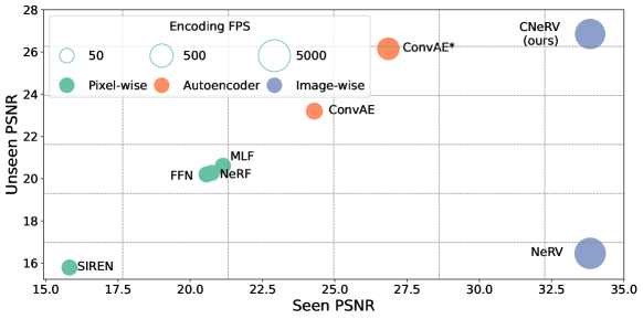
Figure 1: CNeRV achieves the highest unseen PSNR and matches state-of-the-art seen PSNR, at fast encoding speeds. CNeRV and NeRV are image-wise neural representations, ConvAE/ConvAE* are convolutional autoencoders with small/large embedding, respectively; SIREN, FFN, NeRF, and MLF are pixel-wise neural representations.

Visual data compression remains a fundamental problem in computer vision, and most methods can be seen as autoencoders, consisting of two components: encoder and decoder. Traditional compression methods, such as JPEG (Wallace, 1992), H.264 (Wiegand et al., 2003), and HEVC (Sullivan et al., 2012), manually design the encoder and decoder based on discrete cosine transform (DCT) (Ahmed et al., 1974). With the success of deep learning, many attempts (Lu et al., 2019; Rippel et al., 2021; Agustsson et al., 2020; Djelouah et al., 2019; Habibian et al., 2019; Liu et al., 2019, 2021; Rippel et al., 2019; Wu et al., 2018) have been made to replace certain components of existing compression pipelines with neural networks. Although these learning-based compression methods show high potential in terms of rate-distortion performance, they suffer from expensive computation, not just to train, but also to encode and decode. Moreover, as a result of being partially hand-crafted, they are also quite reliant on various hard-coded priors.

To address the heavy computation for autoencoders, implicit neural representations (Rahaman et al., 2019; Sitzmann et al., 2020; Schwarz et al., 2021; Chen and Zhang, 2019; Park et al., 2019) have become popular due to simplicity, compactness, and efficiency. These methods show great potential for visual data compression, such as COIN (Dupont et al., 2021) for image compression, and NeRV (Chen et al., 2021) for video compression. By representing visual data as neural networks, visual data compression problems can be converted to model compression problems and greatly simplify the complex encoding and decoding pipeline.

Unlike other implicit methods that map a single network to a single image, NeRV trains as a single network to map timestamps to RGB frames directly for entire videos. This allows NeRV to achieve incredible results for video compression. However, because NeRV’s input embedding comes from the positional encoding of an image/frame index, which is content-agnostic, NeRV can only memorize. This is evidenced by it achieving surprisingly poor reconstruction quality for unseen data (images/frames that are skipped during training), even when these images only deviate very slightly from images it has seen. This means that NeRV can only work with a fixed set of images that it has seen during training time, and it could never perform, for example, post-training operations such as frame interpolation.

We thus propose Content-adaptive Neural Representation for Visual Data (CNeRV) to enable internal generalization. With a content-adaptive embedding, rather than a temporal/index-based embedding, CNeRV combines the generalizability of autoencoders (AEs) with the simplicity and compactness of implicit representation. Similar to implicit representations, CNeRV has a strong decoder, and stores most of the visual prior in the neural network itself. Given a tiny embedding, CNeRV can reconstruct the image with high quality, just as NeRV does, and serves as an internally-generalizable neural representation, shown in Figure 1.

We summarize our primary contributions as follows:

• We propose content-adaptive embedding (CAE) to effectively and compactly encode visual information, and generalize to skipped images for a given video/domain.

• We propose CNeRV based on CAE, which leverages a single-layer mini-network to encode images ($120\times$ faster than NeRV), with no need for the time-consuming per-image overfitting used by implicit representation methods.

• We demonstrate that CNeRV outperforms autoencoders on the reconstruction task ($+9.5db$ for seen image PSNR, $+3.5db$ for unseen image PSNR).

• We show promising video compression results for both unseen and all frames when compared with traditional visual codec such as H.264 and HEVC.

2 Related Work

Neural Representation. Implicit neural representations can be divided into two types: pixel-wise representation and image-wise representation. Taking pixel coordinate as input, pixel-wise representation yields outputs based on the input queries, and have become popular for numerous applications, including image reconstruction (Sitzmann et al., 2020), shape regression (Chen and Zhang, 2019; Park et al., 2019), and 3D view synthesis (Schwarz et al., 2021). For image-wise implicit representation, NeRV (Chen et al., 2021) outputs the whole image given an index, which greatly speeds up the encoding and decoding process compared to pixel-wise methods, and a recent E-NeRV (Li et al., 2022) improves the architecture design. CNeRV is also an image-wise representation method. As (Mehta et al., 2021) points out, most implicit functional representations rely on fitting to each individual test signal, which can be expensive, even with meta-learning (Tancik et al., 2021) to reduce the amount of regression necessary. Although we focus entirely on image reconstruction, and its relationship with video-related tasks, we select from these methods some suitable baselines that warrant comparison. We choose MLP-based methods which leverage (a) periodic activations, such as SIREN (Sitzmann et al., 2020) and MLF (Modulated Local Functional Representations) (Mehta et al., 2021), and (b) Fourier features, such as NeRF (Mildenhall et al., 2020) and FFN (Fourier Feature Network) (Tancik et al., 2020).

Autoencoders. Our work is related to other works where a network learns to represent an image in a way that either relies on or later lends itself to reconstruction of the image. Of these methods, ours is closely related to auto-encoding (Ahmed et al., 1974; Vincent et al., 2008; Kingma and Welling, 2014; Pu et al., 2016), which focuses on encoding and reconstruction of real images, sometimes by leveraging adversarial techniques (Makhzani et al., 2016; Donahue et al., 2016; Dumoulin et al., 2017; Donahue and Simonyan, 2019) that were originally proposed to help synthesize new images (Goodfellow et al., 2014). Numerous algorithmic and architectural improvements (Chen et al., 2019; Dupont, 2018; van den Oord et al., 2018; Tolstikhin et al., 2019) were introduced later based on the vanilla autoencoder. We take vanilla convolutional autoencoder and convolutional VAE as baselines in this work. In fact, our method is akin to an autoencoder that is optimized for data compression: the encoder is very small and fast, while the decoder is reasonably quick and not excessively large.

Visual Codec. Borrowing principles from image compression techniques (Wallace, 1992; Skodras et al., 2001) and transform coding methods (Ahmed et al., 1974; Antonini et al., 1992), traditional video compression methods such as MPEG (Le Gall, 1991), H.264 (Wiegand et al., 2003), and HEVC (Sullivan et al., 2012) are designed to be both fast and accurate. Recently, deep learning techniques have been proposed to replace portions of the video compression pipeline (Chen et al., 2021; Rippel et al., 2021; Liu et al., 2020; Agustsson et al., 2020; Djelouah et al., 2019; Habibian et al., 2019; Liu et al., 2019, 2021; Rippel et al., 2019; Wu et al., 2018; Khani et al., 2021). Although these learning-based methods show promising results for rate-distortion performance, most of them suffer from complex pipelines and heavy computation. Of all the methods referenced in this section, ours is most closely related NeRV (Chen et al., 2021), which converts frame index to a positional encoding to allow a neural network to memorize and compress a video. Covered in more detail in Sec. 3, a primary difference from NeRV is CNeRV’s use of a content-adaptive embedding, which allows CNeRV to encode frames that were skipped during training time.

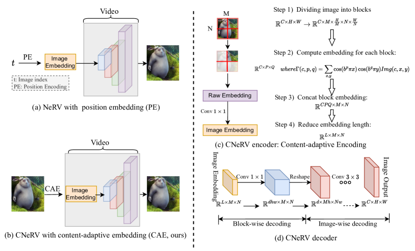
Figure 2: (a) NeRV represents videos or image datasets as neural neworks, taking an image index as input, and outputting the whole image. (b) CNeRV also stores visual priors in neural networks, but by taking a content-adaptive embedding as input, it can easily generalize internally to unseen (skipped) frames. (c) CNeRV encoder first divides the input image into blocks, then computes content-adaptive embedding, and finally reduce the embedding length with a $1\times 1$ convolution. (d) CNeRV decoder consists of block-wise computation ($1\times 1$ convolution) and image-wise computation ($3\times 3$ convolution), more details are in Figure 3.

3 Method

Our work on representation and compression for visual data builds on NeRV. We replace their content-agnostic positional embedding with a proposed content adaptive embedding and a single-layer neural encoder. To clarify the relationship between CNeRV and NeRV, we first revisit NeRV in Sec. 3.1, then present CNeRV to introduce internal generalization in Sec. 3.2, and finally how it can be leveraged for visual data compression in Sec. 3.3.

3.1 Revisiting NeRV

As shown in Figure 2, NeRV takes as input an image index $t$, normalized between $0$ and $1$, and outputs the whole image directly, through an embedding layer and a neural network. The image embedding is given by a positional encoding function:

$$\footnotesize\Gamma(t)=\left(\sin\left(b^{0}\pi t\right),\cos\left(b^{0}\pi t\right),\dots,\sin\left(b^{l-1}\pi t\right),\cos\left(b^{l-1}\pi t\right)\right)$$ (1)

where $t$ is the image index, $b$ is the frequency value, and $l$ is the frequency length. Specifically, the NeRV network, as illustrated in Figure 3(a), consists of a multi-layer perceptron (MLP) and stacked NeRV blocks. To upscale the spatial size, a NeRV block stacks a convolution layer, a pixelshuffle module (Shi et al., 2016), and an activation layer, as illustrated in Figure 3(b).

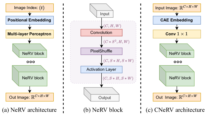
Figure 3: Left: NeRV consists of MLP and NeRV blocks. Middle: NeRV block. Right CNeRV consists of block-wise computation ($1\times 1$ convolution) and image-wise computation (NeRV blocks with $3\times 3$ convolution).

3.2 CNeRV: Content-adaptive Neural Representation for Visual Data

To ameliorate NeRV’s lack of internal generalization (results in supplementary material), motivated by its failure to properly correlate neighboring frames, we propose a different embedding. Rather than a positional encoding, which is content-agnostic, we design a content-aware encoding. We create a single-layer encoder to perform a learned transform on this encoding and use NeRV decoder for reconstruction.

CNeRV Encoder We introduce a tiny, single-layer encoder in Figure 2(c) that uses content-adaptive embedding to achieve internal generalization.

Dividing image into blocks. One insight behind CNeRV is that local visual patterns can be extracted and act as a visual prior. To achieve this, we first divide each input image into blocks and encode them in a batch, illustrated in step $1$ at Figure 2(c), $\mathbb{R}^{C\times H\times W}\rightarrow\mathbb{R}^{C\times M\times\frac{H}{M}\times N\times\frac{W}{N}}$ where $\mathbb{R}^{C\times H\times W}$ represents the input image, $C$ the image channel, $H$ and $W$ image height and width, $M$ and $N$ block numbers

Content-adaptive embedding. To improve the embedding generalization, we encode the image content into an embedding. Inspired by DCT (Ahmed et al., 1974) and positional encoding, we compute content-adaptive embedding $\mathbb{R}^{C\times P\times Q}$ with

$$\footnotesize\Gamma(c,p,q)=\sum_{x,y}\cos(b^{p}\pi x)\cos(b^{q}\pi y)\text{Img}(c,x,y)$$ (2)

where $b$ is the frequency value, $p$ and $q$ are the frequency values, Img($c,x,y$) is the pixel value at location $(x,y)$ for channel $c$, and $x$ and $y$ are normalized between $(0,1)$. We then concatenate the block embedding to construct the image embedding $\mathbb{R}^{CPQ\times M\times N}$ as shown in Figure 2(c) with steps $2$ and $3$.

Reduce embedding dimension. Since the raw embedding can be very high in length dimension ($CPQ$), we introduce a $1\times 1$ convolution to reduce the length and get an embedding $\mathbb{R}^{L\times M\times N}$. This will be the image latent code and also the input of CNeRV decoder, as illustrated in Figure 2(c), step $4$.

CNeRV Decoder We illustrate the CNeRV decoder in Figure 2(d) and divide it into two parts: block-wise and image-wise decoding.

Block-wise Decoding. Given image embedding $\mathbb{R}^{L\times M\times N}$, we firstly decode it block-wisely with $1\times 1$ convolution into $\mathbb{R}^{dhw\times M\times N}$. Then we reshape it into $\mathbb{R}^{d\times Mh\times Nw}$, which means every block embedding $\mathbb{R}^{L\times 1\times 1}$ is decoded into a $\mathbb{R}^{d\times h\times w}$ cube. Since this is shared by blocks, we refer to it as block-wise decoding.

Image-wise Decoding. Given $\mathbb{R}^{d\times Mh\times Nw}$, following NeRV (Chen et al., 2021), we upscale the feature map into the final image output $\mathbb{R}^{C\times H\times W}$ with stacked NeRV blocks. Since NeRV block consists of $3\times 3$ convolution and fuses information over the whole image, we therefore refer to it as image-wise decoding.

Loss Objective Following NeRV (Chen et al., 2021), we adopt a combination of L1 and SSIM loss as our loss function for network optimization, following

$$\footnotesize L=\alpha\left\lVert y-v\right\rVert_{1}+(1-\alpha)(1-\text{SSIM}(y,v))$$ (3)

where $y$ and $v$ are the ground truth image and CNeRV image prediction, and $\alpha$ is a hyperparameter to balance the loss items.

3.3 Application: Visual Data Compression

Following NeRV, we use model pruning, quantization, and entropy encoding for model compression. Similar to model quantization, we also apply embedding quantization for visual data compression. Given a tensor $\mu$, a tensor element $\mu_{i}$ at position $i$ is

$$\footnotesize\mu_{i}=\text{Round}((\mu_{i}-\mu_{\text{min}})/s)*\text{s}+\mu_{\text{min}},\text{where}\quad\text{s}=(\mu_{\text{max}}-\mu_{\text{min}})/2^{\text{bit}}$$ (4)

‘Round’ is a function that rounds to the closest integer, ‘bit’ is the bit length for quantization, $\mu_{\text{max}}$ and $\mu_{\text{min}}$ are the max and min value for $\mu$, and ‘scale’ is the scaling factor. Using this equation, each model parameter or frame embedding value can be represented with only ‘bit’ length – by compressing the model and embedding in this way, we achieve visual data compression. When computing quantized model size, we also use entropy encoding as an off-the-shelf technique to save space.

4 Experiments

Datasets and implementation details We conduct experiments on both video and image datasets. For video, we choose Big Buck Bunny (big, ) (our default dataset), UVG (Mercat et al., 2020), and MCL-JCL (Wang et al., 2016) and list their statistics in Table 6. To make it suitable for generation, we crop the video resolution from $1080\times 1920$ to $960\times 1920$. To evaluate internal generalization on different resolutions, we downsample video to $480\times 960$ (our default resolution) and $240\times 480$. We hold out 1 in every 5 images/frames for testing, and thus have a 20% test split set, referred to as ‘unseen’. We also conduct experiments on Celeb-HQ (Lee et al., 2020), a face dataset with 12k/3k images for seen/unseen set, and Oxford Flowers (Nilsback and Zisserman, 2008), which has 3.3k/1.6k images for seen/unseen set.

For CNeRV architecture on $480\times 960$ videos, the block number $M\times N$ is $2\times 4$, frequency value $b$ is $1.15$ and frequency length $P$ and $Q$ are both $15$, the block embedding length $L$ is $60$, the output size of block-wise decoder $d\times h\times w$ is $620\times 30\times 60$, followed by 4 NeRV blocks, each with an up-scale factor of 2. By changing channel width $d$, we can build CNeRV with different sizes. For the loss objective, from Equation 3, $\alpha$ is set to $0.7$. For NeRV embeddings, we use $b=1.25$ and $l=240$ in Equation 1, following the settings from the original paper. We evaluate the video quality with two metrics: PSNR and MS-SSIM. Bits-per-pixel (BPP) is adopted to evaluate the compression ratio. We implement our method in PyTorch (Paszke et al., 2019) and train it in full precision (FP32), on NVIDIA RTX2080Ti.

We firstly fit the model on the seen split, and evaluate its internal generalization on the unseen set. When computing “total size” for a representation method, for implicit representation (e.g., NeRV) we only compute model parameters, while for methods with image latent code, we compute both model parameters and image embedding size as total size. More results can be found in the supplementary material.

Table 1: Video dataset statistics

Dataset	#frames	#videos	Duration	FPS
UVG	3900	7	5s or 2.5s	120
Bunny	5032	1	$\sim$10min	8
MCL	4115	30	5s	24-30

Table 2: Results on different video datasets

Method	Dataset	Embed Length	Total Size	Seen	PSNR Unseen $\uparrow$	Gap $\downarrow$
NeRV	UVG	480	64M	36.05	23.66	12.39
CNeRV	UVG	480	64M	35.83	28.76	7.07
NeRV	Bunny	480	64M	33.53	16.46	17.07
CNeRV	Bunny	480	64M	33.83	26.85	6.98
NeRV	MCL	480	64M	34.83	19.44	15.39
CNeRV	MCL	480	64M	34.67	26.98	7.69

Table 3: Results on different model sizes

Method	Model Size	Embed Length	Total Size	Seen	PSNR Unseen $\uparrow$	Gap $\downarrow$
NeRV	Small	480	32M	31	16.72	14.28
CNeRV	Small	480	32M	31.33	26.41	4.92
NeRV	Medium	480	64M	33.53	16.46	17.07
CNeRV	Medium	480	64M	33.83	26.85	6.98
NeRV	Large	480	97M	35.32	16.04	19.28
CNeRV	Large	480	97M	35.5	27.08	8.42

Table 4: Results on video resolutions

Method	Video Resolution	Embed Length	Total Size	Seen	PSNR Unseen $\uparrow$	Gap $\downarrow$
NeRV	240*480	480	60M	37.14	16.9	20.24
CNeRV	240*480	480	60M	36.99	27.97	9.02
NeRV	480*960	480	64M	33.53	16.46	17.07
CNeRV	480*960	480	64M	33.83	26.85	6.98
NeRV	960*1920	480	67M	32.06	16.06	16
CNeRV	960*1920	480	67M	32.4	26.15	6.25

Table 5: Results on training data size

Method	Training Images	Embed Length	Total Size	Seen	PSNR Unseen $\uparrow$	Gap $\downarrow$
NeRV	1k	480	64M	34.6	12.57	22.03
CNeRV	1k	480	64M	34.78	26.41	8.37
NeRV	2k	480	64M	33.53	16.46	17.07
CNeRV	2k	480	64M	33.83	26.85	6.98
NeRV	4k	480	64M	32.78	20.68	12.1
CNeRV	4k	480	64M	32.94	27.75	5.19

Table 6: Results on image datasets

Method	Dataset	Embed Length	Total Size	Seen	PSNR Unseen $\uparrow$	Gap $\downarrow$
NeRV	Celeb	240	33M	27.44	11.27	16.17
CNeRV	Celeb	240	33M	27.42	21.34	6.08
NeRV	Flower	240	35M	27	11.29	15.71
CNeRV	Flower	240	36M	27.04	18.54	8.5

Comparison to NeRV We present our main result in Table 6, which shows that CNeRV consistently outperforms NeRV in terms of both reconstruction quality of unseen images (unseen PSNR) and internal generalizability (PSNR gap between seen and unseen frames/images). Extended tables with more details and results in this section can be found in the supplementary material. Note that the generalization of NeRV becomes worse when FPS decreases, i.e., with diversified frame content, while CNeRV retains its generalizability in all cases. We first verify CNeRV’s superior performance holds under a variety of settings, increasing model size in Table 6, various video resolution in Table 6, various training images in Table 6.

We then extend our finding on the non-sequential nature of NeRV’s representation to apply it to an image dataset, using an arbitrary index for each image as the frame index. NeRV thus takes image index (1/N, …, N/N respectively for N images) as input. With this adaptation, we compare them in Table 6 and CNeRV shows superior internal generalization.

There is no question that NeRV and CNeRV both succeed by fitting to their training data. However, as Figure 4 shows, CNeRV is able to do this without sacrificing generalization for increasing training epochs (it does not exhibit the same overfitting behavior). CNeRV’s performance for unseen images doesn’t decrease as training time increases, even though its seen image reconstruction quality continues to improve. Furthermore, Table 7 points out that CNeRV is vastly superior in terms of encoding time for unseen frames, when accounting for the fact that NeRV must be fine-tuned on those previously unseen images to reach competitive PSNR. Thus, CNeRV’s internal generalization allows it to save training/encoding time.

Table 7: Comparison of encoding time. We fine-tune NeRV on unseen images until it reaches comparable PSNR with CNeRV.

Method	Overfit	UVG		Bunny		MCL
		PSNR $\uparrow$	FPS $\uparrow$	PSNR $\uparrow$	FPS $\uparrow$	PSNR $\uparrow$	FPS $\uparrow$
NeRV	✓	28.69	0.13	26.59	0.14	26.75	0.13
CNeRV		28.76	16.1 ($124\times$)	26.85	16.1 ($115\times$)	26.98	16.1 ($124\times$)

Table 8: Compare with Autoencoders and pixel-wise neural representations

Methods	Image- wise	Embed Length	Total Size	Training time	PSNR seen $\uparrow$	PSNR unseen $\uparrow$	Encoder size $\downarrow$	Encoding time $\downarrow$
SIREN (Sitzmann et al., 2020)		480	66M	$2\times$	15.82	15.79	62M	16.9ms
FFN (Tancik et al., 2020)		480	66M	$2\times$	20.69	20.33	62M	16.9ms
NeRF (Mildenhall et al., 2020)		480	66M	$2\times$	21.04	20.56	62M	16.9ms
MLF (Mehta et al., 2021)		480	66M	$2\times$	21.13	20.61	62M	16.9ms
ConvAE	✓	480	68M	$2\times$	24.29	23.2	47M	13.4ms
ConvVAE	✓	480	68M	$2\times$	23.92	21.71	46M	13.7ms
ConvAE*	✓	12k	68M	$2\times$	26.83	26.15	1.9M	2.9ms
CNeRV (ours)	✓	480	64M	$1/6\times$	24.35	23.19	0.4M	0.37ms
CNeRV (ours)	✓	480	64M	$1\times$	33.83	26.85	0.4M	0.37ms

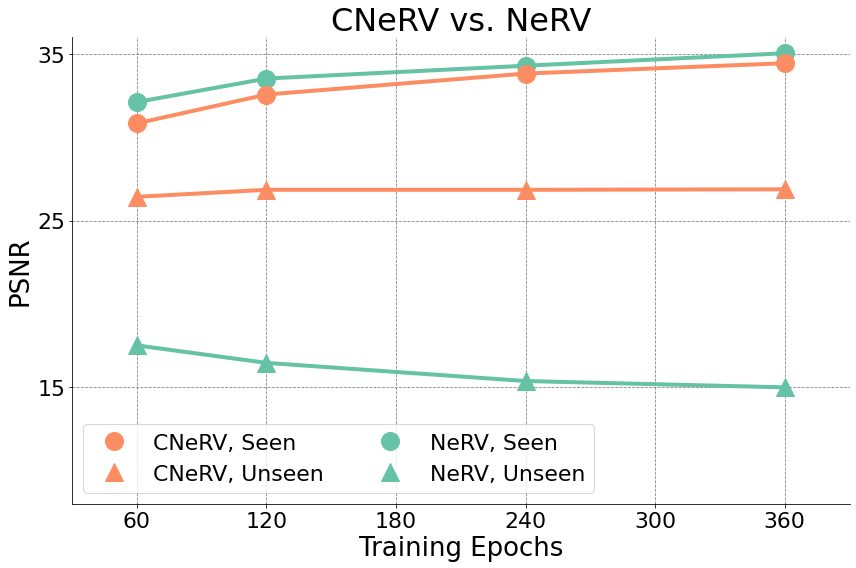
Figure 4: CNeRV keeps increasing seen PSNR and remains stable on unseen PSNR while NeRV’s better seen PSNR comes at the cost of unseen PSNR

Table 9: Decoding speed, frames per second (FPS) reported

Resolution	H.264	H.265	CNeRV
$480\times 960$	85.4	56.3	123.4
$960\times 1920$	24.5	16.2	31.6

Table 10: Interpolation results on different datasets. We show PSNR of unseen images with interpolated and ground truth embedding

Dataset	GT embedding	Embedding interpolation
UVG	28.76	28.88
MCL	26.85	26.33
Bunny	26.98	24.94

Comparison with Other Reconstruction Methods We also compare with autoencoders and pixel-wise neural representations. For autoencoders, we choose the most common convolutional autoencoder and convolutional variational autoencoder as baselines, referred to as ConvAE and ConvVAE. They reduce the image into the same block number as CNeRV (i.e., $2\times 4$) with strided convolution. The block embedding length is the same with CNeRV (i.e., $60$) as well. We also compare with ConvAE* which light neural networks where most visual information is stored in the huge image-specific embedding. For pixel-wise neural representations, we choose NeRF (Mildenhall et al., 2020), SIREN (Sitzmann et al., 2020), FFN (Tancik et al., 2020), and MLF (Mehta et al., 2021) as baselines. Following MLF (Mehta et al., 2021), we train a separate auto-encoder to provide content information besides the coordinate input. For fair comparison, we keep the latent code the same length as CNeRV. All other setups also follow MLF (Mehta et al., 2021).

Table 8 shows reconstruction results for both seen and unseen images, as well as encoder model size and encoding speed. Note that for encoding time, we only consider the forward time, ignoring the data loading overhead. With a tiny encoder and strong decoder, CNeRV outperforms autoencoders and pixel-wise neural representations in many regards, including reconstruction quality of seen and unseen images, and encoding speed. We show visualization results for seen images in Figure 11 and unseen images in Figure 12. With the same embedding length and similar total size, CNeRV outperforms NeRV with better detail, absence of artifacts, and lack of spillover from previous frames. Although autoencoder with large embeddings can reach comparable generalization for unseen images, it struggles a lot for reconstruction of seen images. But, visual differences still exist between CNeRV and ground truth, and future work can focus on mitigating these issues.

Figure 5: Video reconstruction for seen frames from video Bunny. CNeRV results are comparable to NeRV, while autoencoders suffers from bluriness, due to the fact that without implicit representation it cannot perform well in the compression setting (tiny embedding).

Figure 6: Video reconstruction for unseen frames from Bunny. CNeRV results are similar for unseen as for seen, while autoencoders is still significantly blurrier than CNeRV. NeRV suffers from a myriad of failures.

For low reconstruction quality of pixel-wise neural representations, we believe both these methods are designed and optimized for low-resolution images, and a similar performance drop on high-resolution images is also observed in MLF (Mehta et al., 2021). For the ConvAE and ConvVAE, we speculate two potential causes for the inferior reconstruction capacity. First, due to the fact that the parameters are more evenly balanced between encoder and decoder, they rely on larger embeddings and struggle for our embedding size. Second, we speculate that small training datasets likely limit their capability as well. We show in the supplementary material that increasing model size, embedding length, and amount of training data each make autoencoders more competitive with CNeRV.

We also compare decoding speed with traditional codecs in Table 10. The decoding of traditional codecs are measured with 8 CPUs, while CNeRV is measured on 1 RTX2080ti. As a video neural representation, CNeRV shows good decoding advantage due to its simplicity and can be deployed easily.

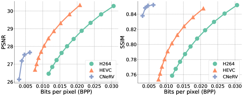
Figure 7: Compression for unseen frames.

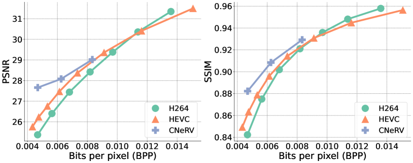
Figure 8: Compression for all frames.

Frame interpolation and Visualization Given neighboring frames are typically similar, we investigate whether using CNeRV to encode unseen frames is better than interpolating from the embeddings of the neighboring seen frames. We show these results in Table 10. Interpolated embeddings achieve similar performance with actual CNeRV embeddings for unseen images across the lower FPS datasets, but significantly lower results for the Bunny dataset. With the same embedding length and similar total size, CNeRV outperforms NeRV and autoencoder with better detail for both seen and unseen frames.

Visual Data Compression We also show visual data compression results for CNeRV, as discussed in Sec. 3.3. We compare the rate-distortion results with traditional visual codec such as H.264 and HEVC. For unseen frames, we compare visual comparison results in Figure 8 where CNeRV bitrates only consider image embedding as all other autoencoder methods do (Rippel et al., 2021; Liu et al., 2020; Agustsson et al., 2020; Djelouah et al., 2019). Besides, we evaluate compression results on the full video (both seen and unseen frames) frames where we combine both the image embedding and model parameters to compute bitrates, CNeRV outperforms H.264 and HEVC on both PSNR and SSIM with similar bpp in Figure 8.

5 Conclusion

In this work, we propose a content-adaptive neural representation, CNeRV. CNeRV combines the generalizability of autoencoders and simplicity and compactness of neural representation. With a single-layer mini-encoder to generate the embedding, CNeRV outperforms autoencoders for the reconstruction task in terms of image quality ($+3.5db$ for unseen image PSNR), encoding speed ($36\times$ faster), and encoder size ($116\times$ smaller). We leverage this content-adaptive embedding with CNeRV to encode unseen images quickly ($120\times$ faster than NeRV), with no need for the time-consuming per-image overfitting. We also show promising visual data compression results and provide embedding analysis.

Acknowledgement. This project was partially funded by an independent grant from Facebook AI and the DARPA SAIL-ON (W911NF2020009) program.

Appendix A More Results

A.1 Embedding Quantization Results

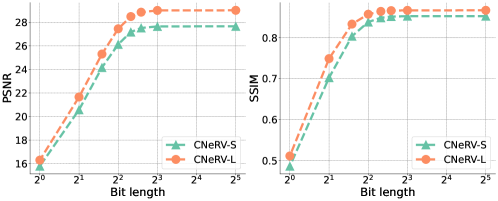
Figure 9: Embedding quantization, We evaluate reconstruction quality on unseen images with embedding quantization.

For unseen frames and with an $8$-bit quantized model, we further quantize the block embedding, ranging from the original $32$ bit to $1$ bit, where where the image embedding can maintain most of its capacity with only $6$ bits in Figure 9

A.2 More Autoencoder Results

We first provide more autoencoder results, where both seen PSNR and unseen PSNR improve as we increase the training images, embedding length, and model size.

Table 11: Autoencoder results with more training images, bigger model size, and longer embeddings.

Methods	Embed Length	Model Size	Training Images	PSNR Seen $\uparrow$	PSNR Unseen $\uparrow$
ConvAE	480	68M	2k	24.29	23.2
ConvAE	1000	68M	4k	26.6	25.92
ConvAE	48k	83M	4k	29.28	29.28

A.3 Sensitivity Analysis and Limitations

Table 12: Frequency value $b$ ablation

Base number	PSNR		MS-SSIM
	Seen $\uparrow$	Unseen $\uparrow$	Seen $\uparrow$	Unseen $\uparrow$
1.05	32.6	25.94	0.915	0.8072
1.15	33.83	26.85	0.9539	0.8242
1.25	33.5	26.67	0.949	0.8217

Table 13: Frequency length ablation

Freq number	PSNR		MS-SSIM
	Seen $\uparrow$	Unseen $\uparrow$	Seen $\uparrow$	Unseen $\uparrow$
10	32.75	26.3	0.9229	0.8151
15	33.83	26.85	0.9539	0.8242
20	34.07	26.84	0.9565	0.8242

Figure 10: Sensitivitiy for Block number

Block number	Embed length	PSNR		MS-SSIM
		Seen $\uparrow$	Unseen $\uparrow$	Seen $\uparrow$	Unseen $\uparrow$
$1\times 2$	480	30.22	25.31	0.8975	0.8059
$2\times 4$	480	33.83	26.85	0.9539	0.8242
$5\times 10$	500	4.7	4.69	0.3344	0.3336
$5\times 10$	1000	34.49	27.63	0.9788	0.8597

We conduct an ablation study on our content-adaptive encoding. For base value $b$ in Equation 2, Table 13 shows that $1.15$ performs better than $1.05$ and $1.25$. For frequency length $P$ and $Q$, Table 13 shows results with $10$, $15$, and $20$. Although $20$ is better for seen PSNR, it does not further improve unseen PSNR and will introduce more encoding computation. Since we mainly focus on internal generalizability in this work, i.e., unseen image PSNR, we choose $15$ as the default frequency length. For block numbers, Table 10 shows results for $1\times 2$, $2\times 4$, and $5\times 10$. where total embedding length is computed by $M\times N\times L$. With $2\times 4$ blocks, CNeRV reaches the best performance for both seen and unseen images. Note that when embedding length is too short (e.g., 10 for block number $5\times 10$), CNeRV fails to overfit; nevertheless, it can still perform reasonable reconstruction.

Limitation The main limitation of our method is that with a small training dataset, unseen PSNR still lags behind seen PSNR. Although more training images can alleviate this problem, CNeRV still cannot reconstruct unseen images with perfect fidelity in this work. This also limits its application for visual codec or compression methods.

A.4 More visualization results

Figure 11: Video compression results for seen frames from video Bunny. Note that CNeRV results are comparable to NeRV, while autoencoders suffers from bluriness, due to the fact that without implicit representation it cannot perform well in the compression setting (tiny embedding).

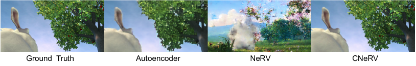
Figure 12: Video compression results for unseen frames from Bunny. CNeRV results are similar for unseen as for seen, while autoencoders is still significantly blurrier than CNeRV. NeRV suffers from a myriad of failures.

We show visualization results for seen images in Figure 11 and unseen images in Figure 12. With the same embedding length and similar total size, CNeRV outperforms NeRV with better detail, absence of artifacts, and lack of spillover from previous frames. Although autoencoder with large embeddings can reach comparable generalization for unseen images, it struggles a lot for reconstruction of seen images. But, visual differences still exist between CNeRV and ground truth, and future work can focus on mitigating these issues. We provide more visualization results in a separate folder named ‘cnerv_visualization’, you can easily access them through the ‘index.html’.

A.5 NeRV Generalization Results

We provide more NeRV results on shuffled/sequential video frames in Table 14, with different number of training images on ‘Big Buck Bunny’.

Table 14: NeRV performance with shuffled frame index. It shows that the input embedding of frame index does not provide any meaningful information since shuffling the data does not impact the final performance.

	Dataset Size	PSNR		MS-SSIM
		Seen $\uparrow$	Unseen $\uparrow$	Seen$\uparrow$	Unseen $\uparrow$
Sequential	1k	34.6	12.57	0.9489	0.3495
Shuffle	1k	35.22	13.15	0.9554	0.3905
Sequential	2k	33.53	16.46	0.919	0.4933
Shuffle	2k	33.47	16.36	0.9193	0.4841
Sequential	4k	32.78	20.68	0.9077	0.6994
Shuffle	4k	32.45	20.24	0.9073	0.6859

A.6 Embedding interpolation

Table 15: Interpolation results on different datasets. We show PSNR of unseen images with pixel interpolation and embedding interpolation. Besides, we also show results of ground truth embedding

Dataset	Pixel Interpolation	GT Embedding	Embedding Interpolation
UVG	30.14	28.76	28.88
MCL	28.05	26.85	26.33
Bunny	27.64	26.98	24.94

We first provide interpolation results in pixel space and embedding space, together with ground truth embedding results, as shown in Table 15. Note that our interpolated embedding shows comparable PSNR with ground truth embedding on unseen images, which clearly demonstrates the internal generalization of our content-adaptive embedding.

A.7 Main Results with MS-SSIM

We also provide a detailed main results, with MS-SSIM, in Table  20,  20,  20,  20, and  20.

Table 16: Results on different video datasets

Method	Dataset	Embed Length	Total Size	Seen	PSNR Unseen $\uparrow$	Gap $\downarrow$	Seen	MS-SSIM Unseen $\uparrow$	Gap $\downarrow$
NeRV	UVG	480	64M	36.05	23.66	12.39	0.9823	0.7314	0.2509
CNeRV	UVG	480	64M	35.83	28.76	7.07	0.9789	0.8739	0.105
NeRV	Bunny	480	64M	33.53	16.46	17.07	0.919	0.4933	0.4257
CNeRV	Bunny	480	64M	33.83	26.85	6.98	0.9539	0.8242	0.1297
NeRV	MCL	480	64M	34.83	19.44	15.39	0.9815	0.5824	0.3991
CNeRV	MCL	480	64M	34.67	26.98	7.69	0.978	0.8229	0.1551

Table 17: Results on different model sizes

Method	Model Size	Embed Length	Total Size	Seen	PSNR Unseen $\uparrow$	Gap $\downarrow$	Seen	MS-SSIM Unseen $\uparrow$	Gap $\downarrow$
NeRV	Small	480	32M	31	16.72	14.28	0.8977	0.5289	0.3688
CNeRV	Small	480	32M	31.33	26.41	4.92	0.911	0.8198	0.0912
NeRV	Medium	480	64M	33.53	16.46	17.07	0.919	0.4933	0.4257
CNeRV	Medium	480	64M	33.83	26.85	6.98	0.9539	0.8242	0.1297
NeRV	Large	480	97M	35.32	16.04	19.28	0.9485	0.4737	0.4748
CNeRV	Large	480	97M	35.5	27.08	8.42	0.9682	0.8235	0.1447

Table 18: Results on different video resolutions

Method	Video Resolution	Embed Length	Total Size	Seen	PSNR Unseen $\uparrow$	Gap $\downarrow$	Seen	MS-SSIM Unseen $\uparrow$	Gap $\downarrow$
NeRV	240*480	480	60M	37.14	16.9	20.24	0.9929	0.5142	0.4787
CNeRV	240*480	480	60M	36.99	27.97	9.02	0.9923	0.8532	0.1391
NeRV	480*960	480	64M	33.53	16.46	17.07	0.919	0.4933	0.4257
CNeRV	480*960	480	64M	33.83	26.85	6.98	0.9539	0.8242	0.1297
NeRV	960*1920	480	67M	32.06	16.06	16	0.902	0.5496	0.3524
CNeRV	960*1920	480	67M	32.4	26.15	6.25	0.9057	0.8118	0.0939

Table 19: Results on different training data size

Method	Training Images	Embed Length	Total Size	Seen	PSNR Unseen $\uparrow$	Gap $\downarrow$	Seen	MS-SSIM Unseen $\uparrow$	Gap $\downarrow$
NeRV	1k	480	64M	34.6	12.57	22.03	0.9489	0.3495	0.5994
CNeRV	1k	480	64M	34.78	26.41	8.37	0.9754	0.813	0.1624
NeRV	2k	480	64M	33.53	16.46	17.07	0.919	0.4933	0.4257
CNeRV	2k	480	64M	33.83	26.85	6.98	0.9539	0.8242	0.1297
NeRV	4k	480	64M	32.78	20.68	12.1	0.9077	0.6994	0.2083
CNeRV	4k	480	64M	32.94	27.75	5.19	0.9274	0.8396	0.0878

Table 20: Results on different image datasets

Method	Dataset	Embed Length	Total Size	Seen	PSNR Unseen $\uparrow$	Gap $\downarrow$	Seen	MS-SSIM Unseen $\uparrow$	Gap $\downarrow$
NeRV	Celeb	240	33M	27.44	11.27	16.17	0.9548	0.4397	0.5151
CNeRV	Celeb	240	33M	27.42	21.34	6.08	0.9536	0.7879	0.1657
NeRV	Flower	240	35M	27	11.29	15.71	0.9028	0.2538	0.649
CNeRV	Flower	240	36M	27.04	18.54	8.5	0.91	0.5491	0.3609

A.8 Embedding Analysis

We also perform 3 measurements to compare the embeddings produced by CNeRV to prior work. We compute uniformity to examine the distribution of each set of embeddings on the hypersphere (wang2020understanding).

$$U=\text{log}\mathop{\mathbb{E}}_{x,y\sim p_{\text{data}}}\left[e^{-t||(||f(x)||_{2}-||f(y)||_{2})||_{2}^{2}}\right]$$ (5)

With the same metric, we compute distances between neighbors for each method, to measure the extent to which each method encodes similar representations for neighboring frames. We also compute normalized distance, which is the neighbor distance (average distance between neighboring embeddings) divided by the uniformity (average distance between all embeddings). This normalized distance gives a more accurate reflection of the extent to which a given method’s embeddings reflect a semantic connection between neighboring frames.

We compute linear centered kernel alignment (CKA) (JMLR:v13:cortes12a) to compare the similarity between embeddings of different methods in a pairwise fashion, as introduced by (pmlr-v97-kornblith19a). To compute this, we first obtain the matrices containing the embeddings for two different methods, such as NeRV and CNeRV, which we represent $X$ and $Y$. We then compute the Gram matrices of the embedding matrices: $K$ = $XX^{T}$, $L$ = $YY^{T}$. The CKA value is given by the normalized Hilbert-Schmidt Independence Criterion (HSIC) (gretton2007kernel) in Equation 6.

$$\text{CKA}(K,L)=\frac{\text{HSIC}(K,L)}{\sqrt{\text{HSIC}(K,K)\text{HSIC}(L,L)}}$$ (6)

Table 21: Embedding distribution on hypersphere. CNeRV embeddings tend to cluster very tightly together, with low uniformity compared to other methods. CNeRV neighbor frame embeddings are still reasonably close together, in stark contrast to NeRV.

Methods	Uniformity			Neighbor	Normalized
	Seen $\downarrow$	Unseen $\downarrow$	All $\downarrow$	Distance $\downarrow$	Distance $\downarrow$
FFN (Tancik et al., 2020)	1.18	1.17	1.18	0.09	0.07
NeRF (Mildenhall et al., 2020)	1.46	1.46	1.46	0.10	0.07
MLF (Mehta et al., 2021)	1.39	1.38	1.38	0.14	0.10
ConvAE	2.00	1.97	1.99	0.14	0.07
ConvVAE	2.71	2.71	2.71	0.21	0.08
NeRV (Chen et al., 2021)	3.97	3.96	3.97	3.60	0.91
CNeRV	0.23	0.23	0.23	0.03	0.15

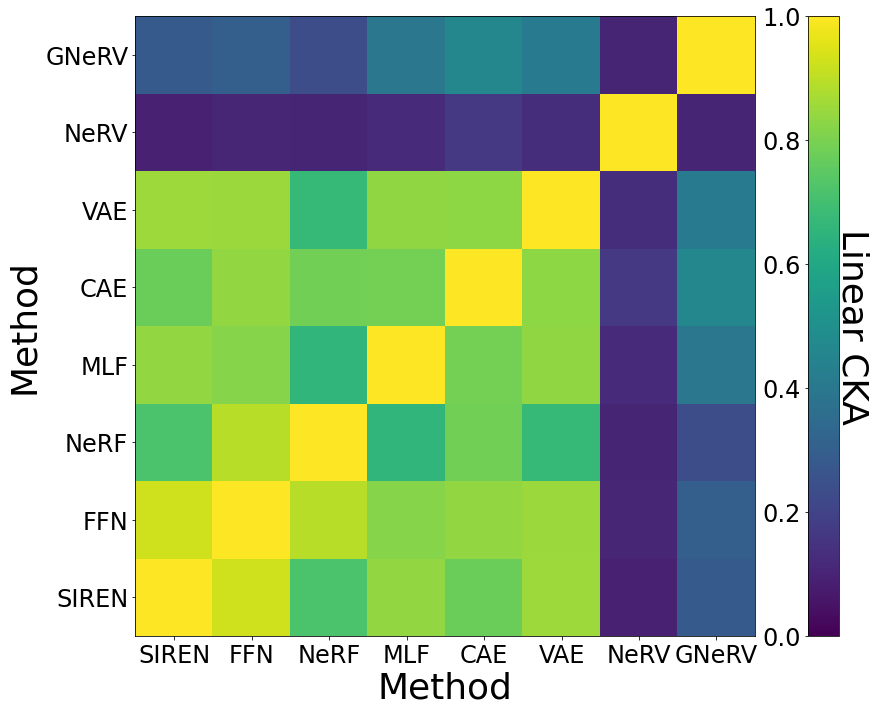
Figure 13: Embedding similarity for methods in Table 8. Embeddings of NeRV and CNeRV are quite different from other methods.

As Table 21 shows, while CNeRV’s content adaptive embeddings are more tightly clustered than the embeddings for the other methods, CNeRV’s neighboring embeddings are still relatively close to each other. CNeRV thus utilizes very little of the embedding space to generate meaningful and generalizable embeddings, and this is also consistent with embedding quantization results as in Figure 9.

Figure 13 further reflects the difference between CNeRV embeddings and those of other methods. Whereas the convolutional autoencoders and the pixel-wise neural representations generate somewhat similar embeddings, CNeRV is quite unique by contrast. This shows how radically different our method is from those already in the literature, in spite of its comparable performance and desirable properties.

References

- (1) Big buck bunny, sunflower version. http://bbb3d.renderfarming.net/download.html. Accessed: 2010-09-30.
- Agustsson et al. (2020) Eirikur Agustsson, David Minnen, Nick Johnston, Johannes Balle, Sung Jin Hwang, and George Toderici. Scale-space flow for end-to-end optimized video compression. In Proceedings of the IEEE/CVF Conference on Computer Vision and Pattern Recognition (CVPR), June 2020.
- Ahmed et al. (1974) N. Ahmed, T. Natarajan, and K.R. Rao. Discrete cosine transform. IEEE Transactions on Computers, C-23(1):90–93, 1974. 10.1109/T-C.1974.223784.
- Antonini et al. (1992) Marc Antonini, Michel Barlaud, Pierre Mathieu, and Ingrid Daubechies. Image Coding Using Wavelet Transform. IEEE Transactions on Image Processing, 1(2):205–220, April 1992.
- Chen et al. (2021) Hao Chen, Bo He, Hanyu Wang, Yixuan Ren, Ser-Nam Lim, and Abhinav Shrivastava. Nerv: Neural representations for videos, 2021.
- Chen et al. (2019) Pengfei Chen, Guangyong Chen, and Shengyu Zhang. Log hyperbolic cosine loss improves variational auto-encoder, 2019.
- Chen and Zhang (2019) Zhiqin Chen and Hao Zhang. Learning implicit fields for generative shape modeling. In Proceedings of the IEEE/CVF Conference on Computer Vision and Pattern Recognition (CVPR), June 2019.
- Djelouah et al. (2019) Abdelaziz Djelouah, Joaquim Campos, Simone Schaub-Meyer, and Christopher Schroers. Neural inter-frame compression for video coding. In Proceedings of the IEEE/CVF International Conference on Computer Vision (ICCV), October 2019.
- Donahue and Simonyan (2019) Jeff Donahue and Karen Simonyan. Large scale adversarial representation learning, 2019.
- Donahue et al. (2016) Jeff Donahue, Philipp Krähenbühl, and Trevor Darrell. Adversarial feature learning. CoRR, abs/1605.09782, 2016.
- Dumoulin et al. (2017) Vincent Dumoulin, Ishmael Belghazi, Ben Poole, Olivier Mastropietro, Alex Lamb, Martin Arjovsky, and Aaron Courville. Adversarially learned inference, 2017.
- Dupont (2018) Emilien Dupont. Learning disentangled joint continuous and discrete representations, 2018.
- Dupont et al. (2021) Emilien Dupont, Adam Goliński, Milad Alizadeh, Yee Whye Teh, and Arnaud Doucet. Coin: Compression with implicit neural representations. arXiv preprint arXiv:2103.03123, 2021.
- Goodfellow et al. (2014) Ian J. Goodfellow, Jean Pouget-Abadie, Mehdi Mirza, Bing Xu, David Warde-Farley, Sherjil Ozair, Aaron C. Courville, and Yoshua Bengio. Generative adversarial nets. In NIPS, pages 2672–2680, 2014.
- Habibian et al. (2019) Amirhossein Habibian, Ties van Rozendaal, Jakub M. Tomczak, and Taco S. Cohen. Video compression with rate-distortion autoencoders. In Proceedings of the IEEE/CVF International Conference on Computer Vision (ICCV), October 2019.
- Khani et al. (2021) Mehrdad Khani, Vibhaalakshmi Sivaraman, and Mohammad Alizadeh. Efficient video compression via content-adaptive super-resolution. arXiv preprint arXiv:2104.02322, 2021.
- Kingma and Welling (2014) Diederik P Kingma and Max Welling. Auto-encoding variational bayes, 2014.
- Le Gall (1991) Didier Le Gall. Mpeg: A video compression standard for multimedia applications. Commun. ACM, 34(4):46–58, April 1991. ISSN 0001-0782. 10.1145/103085.103090.
- Lee et al. (2020) Cheng-Han Lee, Ziwei Liu, Lingyun Wu, and Ping Luo. Maskgan: Towards diverse and interactive facial image manipulation. In IEEE Conference on Computer Vision and Pattern Recognition (CVPR), 2020.
- Li et al. (2022) Zizhang Li, Mengmeng Wang, Huaijin Pi, Kechun Xu, Jianbiao Mei, and Yong Liu. E-nerv: Expedite neural video representation with disentangled spatial-temporal context. ECCV, 2022.
- Liu et al. (2019) Haojie Liu, Tong Chen, Ming Lu, Qiu Shen, and Zhan Ma. Neural video compression using spatio-temporal priors, 2019.
- Liu et al. (2021) Haojie Liu, Ming Lu, Zhan Ma, Fan Wang, Zhihuang Xie, Xun Cao, and Yao Wang. Neural video coding using multiscale motion compensation and spatiotemporal context model. IEEE Transactions on Circuits and Systems for Video Technology, 31(8):3182–3196, 2021. 10.1109/TCSVT.2020.3035680.
- Liu et al. (2020) Jerry Liu, Shenlong Wang, Wei-Chiu Ma, Meet Shah, Rui Hu, Pranaab Dhawan, and Raquel Urtasun. Conditional entropy coding for efficient video compression. In Andrea Vedaldi, Horst Bischof, Thomas Brox, and Jan-Michael Frahm, editors, Computer Vision – ECCV 2020. Springer International Publishing, 2020.
- Lu et al. (2019) Guo Lu, Wanli Ouyang, Dong Xu, Xiaoyun Zhang, Chunlei Cai, and Zhiyong Gao. Dvc: An end-to-end deep video compression framework. In Proceedings of the IEEE/CVF Conference on Computer Vision and Pattern Recognition, pages 11006–11015, 2019.
- Makhzani et al. (2016) Alireza Makhzani, Jonathon Shlens, Navdeep Jaitly, Ian Goodfellow, and Brendan Frey. Adversarial autoencoders, 2016.
- Mehta et al. (2021) Ishit Mehta, Michaël Gharbi, Connelly Barnes, Eli Shechtman, Ravi Ramamoorthi, and Manmohan Chandraker. Modulated periodic activations for generalizable local functional representations, 2021.
- Mercat et al. (2020) Alexandre Mercat, Marko Viitanen, and Jarno Vanne. Uvg dataset: 50/120fps 4k sequences for video codec analysis and development. In Proceedings of the 11th ACM Multimedia Systems Conference, pages 297–302, 2020.
- Mildenhall et al. (2020) Ben Mildenhall, Pratul P. Srinivasan, Matthew Tancik, Jonathan T. Barron, Ravi Ramamoorthi, and Ren Ng. Nerf: Representing scenes as neural radiance fields for view synthesis, 2020.
- Nilsback and Zisserman (2008) Maria-Elena Nilsback and Andrew Zisserman. Automated flower classification over a large number of classes. In 2008 Sixth Indian Conference on Computer Vision, Graphics & Image Processing, pages 722–729. IEEE, 2008.
- Park et al. (2019) Jeong Joon Park, Peter Florence, Julian Straub, Richard Newcombe, and Steven Lovegrove. Deepsdf: Learning continuous signed distance functions for shape representation. In Proceedings of the IEEE/CVF Conference on Computer Vision and Pattern Recognition (CVPR), June 2019.
- Paszke et al. (2019) Adam Paszke, Sam Gross, Francisco Massa, Adam Lerer, James Bradbury, Gregory Chanan, Trevor Killeen, Zeming Lin, Natalia Gimelshein, Luca Antiga, Alban Desmaison, Andreas Kopf, Edward Yang, Zachary DeVito, Martin Raison, Alykhan Tejani, Sasank Chilamkurthy, Benoit Steiner, Lu Fang, Junjie Bai, and Soumith Chintala. Pytorch: An imperative style, high-performance deep learning library. In H. Wallach, H. Larochelle, A. Beygelzimer, F. d'Alché-Buc, E. Fox, and R. Garnett, editors, Advances in Neural Information Processing Systems 32, pages 8024–8035. Curran Associates, Inc., 2019.
- Pu et al. (2016) Yunchen Pu, Zhe Gan, Ricardo Henao, Xin Yuan, Chunyuan Li, Andrew Stevens, and Lawrence Carin. Variational autoencoder for deep learning of images, labels and captions. In D. Lee, M. Sugiyama, U. Luxburg, I. Guyon, and R. Garnett, editors, Advances in Neural Information Processing Systems, volume 29. Curran Associates, Inc., 2016.
- Rahaman et al. (2019) Nasim Rahaman, Aristide Baratin, Devansh Arpit, Felix Draxler, Min Lin, Fred Hamprecht, Yoshua Bengio, and Aaron Courville. On the spectral bias of neural networks. In Kamalika Chaudhuri and Ruslan Salakhutdinov, editors, Proceedings of the 36th International Conference on Machine Learning, volume 97 of Proceedings of Machine Learning Research, pages 5301–5310. PMLR, 09–15 Jun 2019.
- Rippel et al. (2019) Oren Rippel, Sanjay Nair, Carissa Lew, Steve Branson, Alexander G. Anderson, and Lubomir Bourdev. Learned video compression. In Proceedings of the IEEE/CVF International Conference on Computer Vision (ICCV), October 2019.
- Rippel et al. (2021) Oren Rippel, Alexander G. Anderson, Kedar Tatwawadi, Sanjay Nair, Craig Lytle, and Lubomir Bourdev. Elf-vc: Efficient learned flexible-rate video coding, 2021.
- Schwarz et al. (2021) Katja Schwarz, Yiyi Liao, Michael Niemeyer, and Andreas Geiger. Graf: Generative radiance fields for 3d-aware image synthesis, 2021.
- Shi et al. (2016) Wenzhe Shi, Jose Caballero, Ferenc Huszar, Johannes Totz, Andrew P. Aitken, Rob Bishop, Daniel Rueckert, and Zehan Wang. Real-time single image and video super-resolution using an efficient sub-pixel convolutional neural network. In Proceedings of the IEEE Conference on Computer Vision and Pattern Recognition (CVPR), June 2016.
- Sitzmann et al. (2020) Vincent Sitzmann, Julien N. P. Martel, Alexander W. Bergman, David B. Lindell, and Gordon Wetzstein. Implicit neural representations with periodic activation functions, 2020.
- Skodras et al. (2001) A. Skodras, C. Christopoulos, and T. Ebrahimi. The jpeg 2000 still image compression standard. IEEE Signal Processing Magazine, 18(5):36–58, 2001. 10.1109/79.952804.
- Sullivan et al. (2012) Gary J. Sullivan, Jens-Rainer Ohm, Woo-Jin Han, and Thomas Wiegand. Overview of the high efficiency video coding (hevc) standard. IEEE Transactions on Circuits and Systems for Video Technology, 22(12):1649–1668, 2012. 10.1109/TCSVT.2012.2221191.
- Tancik et al. (2020) Matthew Tancik, Pratul P. Srinivasan, Ben Mildenhall, Sara Fridovich-Keil, Nithin Raghavan, Utkarsh Singhal, Ravi Ramamoorthi, Jonathan T. Barron, and Ren Ng. Fourier features let networks learn high frequency functions in low dimensional domains, 2020.
- Tancik et al. (2021) Matthew Tancik, Ben Mildenhall, Terrance Wang, Divi Schmidt, Pratul P. Srinivasan, Jonathan T. Barron, and Ren Ng. Learned initializations for optimizing coordinate-based neural representations, 2021.
- Tolstikhin et al. (2019) Ilya Tolstikhin, Olivier Bousquet, Sylvain Gelly, and Bernhard Schoelkopf. Wasserstein auto-encoders, 2019.
- van den Oord et al. (2018) Aaron van den Oord, Oriol Vinyals, and Koray Kavukcuoglu. Neural discrete representation learning, 2018.
- Vincent et al. (2008) Pascal Vincent, Hugo Larochelle, Yoshua Bengio, and Pierre-Antoine Manzagol. Extracting and composing robust features with denoising autoencoders. ICML ’08, New York, NY, USA, 2008. Association for Computing Machinery. ISBN 9781605582054.
- Wallace (1992) G.K. Wallace. The jpeg still picture compression standard. IEEE Transactions on Consumer Electronics, 38(1):xviii–xxxiv, 1992. 10.1109/30.125072.
- Wang et al. (2016) Haiqiang Wang, Weihao Gan, Sudeng Hu, Joe Yuchieh Lin, Lina Jin, Longguang Song, Ping Wang, Ioannis Katsavounidis, Anne Aaron, and C-C Jay Kuo. Mcl-jcv: a jnd-based h. 264/avc video quality assessment dataset. In 2016 IEEE International Conference on Image Processing (ICIP), pages 1509–1513. IEEE, 2016.
- Wiegand et al. (2003) T. Wiegand, G.J. Sullivan, G. Bjontegaard, and A. Luthra. Overview of the h.264/avc video coding standard. IEEE Transactions on Circuits and Systems for Video Technology, 13(7):560–576, 2003. 10.1109/TCSVT.2003.815165.
- Wu et al. (2018) Chao-Yuan Wu, Nayan Singhal, and Philipp Krahenbuhl. Video compression through image interpolation. In Proceedings of the European Conference on Computer Vision (ECCV), September 2018.