Iteration Complexity of Fixed-Step Methods by Nesterov and Polyak for Convex Quadratic Functions

Abstract

This note considers the momentum method by Polyak and the accelerated gradient method by Nesterov, both without line search but with fixed step length applied to strictly convex quadratic functions assuming that exact gradients are used and appropriate upper and lower bounds for the extreme eigenvalues of the Hessian matrix are known. Simple 2-d-examples show that the Euclidean distance of the iterates to the optimal solution is non-monotone. In this context an explicit bound is derived on the number of iterations needed to guarantee a reduction of the Euclidean distance to the optimal solution by a factor $\epsilon$. For both methods the bound is optimal up to a constant factor, it complements earlier asymptotically optimal results for the momentum method, and it establishes another link of the momentum method and Nesterov’s accelerated gradient method.

Key words: Momentum method, convex quadratic optimization, iteration complexity

1. Introduction

Let $f:{\mathbb{R}}^{n}\to{\mathbb{R}}$ be a strictly convex quadratic function. For the minimization of $f$ starting at an initial point $x^{0}\in{\mathbb{R}}^{n}$ with negative gradient $m^{0}:=-\nabla f(x^{0})$ the following “Momentum Method” is considered for $k\geq 0$:

$$x^{k+1}=x^{k}+\alpha m^{k},\qquad m^{k+1}=\beta m^{k}-\nabla f(x^{k+1}).$$

Here $\alpha>0$ is a sufficiently small step length that will be analyzed below and $\beta\in[0,1)$ is a parameter that determines how much of the previous search direction will be added to the new search direction. This parameter is also discussed below.

As pointed out for example in [16], with the initialization $x^{-1}:=x^{0}$ the Momentum Method $(MM)$ is equivalent to the “Heavy Ball Method” ([15]):

$$x^{k+1}=x^{k}-\alpha\nabla f(x^{k})+\beta(x^{k}-x^{k-1}).$$

In spite of the proof of asymptotic optimality of the momentum method $(MM)$ established almost 60 years ago in [15] this method has not received due attention until recently in the context of machine learning and neural networks. It has proved to be very efficient in numerical implementations, also when the gradients are replaced with approximate stochastic gradients, see e.g. [2, 16]. Today modifications of the $(MM)$ are widely used, in particular also in machine learning libraries.

While being efficient in practice, the convergence behavior of momentum methods is “somewhat irregular”. Figure 1 shows a typical non-monotone convergence behavior of the $(MM)$ for the simple 2-d-example $f(x)\equiv\tfrac{1}{2}(x_{1}^{2}+100x_{2}^{2})$ with $\beta=0.85$ and $\alpha=\tfrac{1.9}{100}$ during the first 100 iterations for the initial values $x^{0}=(\tfrac{1}{100},1)^{\text{T}}$, $x^{0}=(1,1)^{\text{T}}$, and $x^{0}=(100,1)^{\text{T}}$.

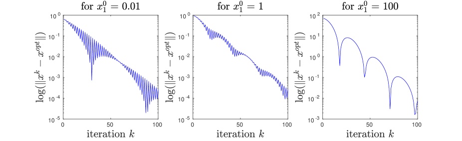
Figure 1: Convergence of the $(MM)$ for a 2-d-example with $\beta=0.85$, and $\alpha=1.9$.

For convex quadratic functions the iterative process $(MM)$ or $(HBM)$ can be written as a recursion with a fixed matrix $M$, and the spectral radius of $M$ is the main factor determining the convergence behavior. A secondary factor is the approximation of the spectral radius by a matrix norm. The connection of both factors and the implication on the choice of parameters is addressed in this paper.

Closely related to the $(MM)$ is Nesterov’s accelerated gradient method [13]. Following the presentation in [14] (Theorem 2.2.3), it can be written as follows: Given $x^{0}\in{\mathbb{R}}^{n}$ set $y^{0}:=x^{0}$ and for $k\geq 0$:

$$x^{k+1}:=y^{k+1}+\beta(y^{k+1}-y^{k})\qquad\hbox{where}\qquad y^{k+1}:=x^{k}-\alpha\nabla f(x^{k})$$

for suitable parameters $\alpha,\beta>0$. As observed in [18], for example, this method falls in the same general framework as $(MM)$: Indeed, by eliminating the variable $y^{k}$ and setting $x^{-1}:=x^{0}$, the iteration $(NAG)$ can also be written in the following compact form,

$$x^{k+1}:=x^{k}-\alpha\nabla f(x^{k})+\beta\left(x^{k}-x^{k-1}-\alpha(\nabla f(x^{k})-\nabla f(x^{k-1}))\right),$$ (1)

where in contrast to $(HBM)$ the momentum term not only includes the previous iterates $x^{k}$ but also the previous descent steps “$-\alpha\nabla f(x^{k})$”. (To obtain the identical initilization as in $(NAG)$, in the very first step $\nabla f(x^{-1})$ needs to be replaced with $0$.)

1.1 Main Results

The main theoretical result of this paper is summarized in the following theorem.

Theorem 1

Let $f:{\mathbb{R}}^{n}\to{\mathbb{R}}$ be a strictly convex quadratic function with minimizer $x^{*}$ and denote $H:=\nabla^{2}f(x^{*})$. Let $\overline{m}$ be an upper bound for the eigenvalues of $H$ and let $0<\underline{m}$ be a lower bound for the eigenvalues of $H$. Then $\overline{\hbox{\rm con}}\hbox{\rm d}(H):=\overline{m}/\underline{m}$ is an upper bound for the condition number of $H$. Assume that $\overline{\hbox{\rm con}}\hbox{\rm d}(H)\geq 28$.

In $(HBM)$ define $\alpha=2/\overline{m}$,  $\beta=\left(1-\sqrt{2\ /\ \overline{\hbox{\rm con}}\hbox{\rm d}(H)}\right)^{2}$ and let $\epsilon\leq 1\,/\,\overline{\hbox{\rm con}}\hbox{\rm d}(H)$ be given. Then, given $x^{0}\in{\mathbb{R}}^{n}$, after

$$1+\lceil\sqrt{2\ \overline{\hbox{\rm con}}\hbox{\rm d}(H)}\ \ln(\tfrac{2}{\epsilon})\rceil$$

steps of the $(HBM)$, an approximate solution $\bar{x}^{k}:=\tfrac{1}{2}(x^{k-1}+x^{k})$ is generated with

$$\|\bar{x}^{k}-x^{*}\|_{2}\leq\epsilon\|x^{0}-x^{*}\|_{2}.$$

A corollary of the analysis of the $(MM)$ is the following well known observation (see [8], for example): It may seem intuitive that with the use of a momentum $\beta>0$, the step length $\alpha$ in $(MM)$ needs to be chosen more carefully. However, at least for the minimization of convex quadratic functions and in the absence of noise, the opposite is true: “If the step itself is made longer by adding more of the previous search step to the new step (i.e. by increasing $\beta\in[0,1)$) then also the step length can be made longer while maintaining global convergence.”

When $\overline{m}$ and $\underline{m}$ are known, then – as detailed in Section 2.6 – the analysis for $(MM)$ also applies to $(NAG)$, and for an appropriate choice of $\alpha,\beta$, an iteration complexity can be established for $(NAG)$ that is a factor $\sqrt{2}$ higher than the bound for $(MM)$ in Theorem 1. The factor $\sqrt{2}$ arises since the step length is reduced by a factor 2 – which essentially amounts to an increase of the estimate $\overline{\hbox{\rm con}}\hbox{\rm d}(H)$ by a factor 2.

1.2 Related work

The paper [15] establishes for $(HBM)$ applied to (non-quadratic smooth) strictly convex functions local convergence of the form

$$\|x-x^{*}\|_{2}\leq c(\epsilon)(1-{\color[rgb]{0,0,0}\tfrac{2}{1+\sqrt{\overline{\hbox{\rm con}}\hbox{\rm d}(H)}}}+\epsilon)^{k}\sqrt{\|x^{1}-x^{*}\|_{2}^{2}+\|x^{0}-x^{*}\|_{2}^{2}}$$

where $c(\epsilon)$ is a constant that only depends on $\epsilon$ (Theorem 9, Statement (3)). This result is obtained by analyzing the spectral condition of a recursion associated with $(HBM)$ and using the fact that for a given matrix there always is a vector norm and an associated matrix norm that approximates the spectral radius to a given precision $\epsilon>0$.

For the case of convex quadratic functions the constant $c(\epsilon)$ is worked out explicitly in a slightly different setting in [8].

The step length in Theorem 1 is limited such that the first step is guaranteed not to increase the function value. For larger values of $\overline{\hbox{\rm con}}\hbox{\rm d}(H)$ the optimal step length $\alpha$ in [15, 8] is nearly twice as long and leads to a substantial increase of the error components associated with large eigenvalues of $H$ during the first several iterations. (This increase can be reduced by taking at most half the step length of [15, 8] in the first iteration, a strategy that also applies to methods with restart.) As the generalization to non-quadratic functions also calls for a shorter step length ([7], Footnote 3) and since the use of long steps leads to an amplification of the stochastic error associated with an inexact evaluation of the gradient, subsequently, only step lengths at most $2/\overline{m}$ are considered in this paper. This imposes a restriction on $\alpha$ cutting off the optimal step lengths identified in [15, 8] at the expense of a small constant factor in the theoretical efficiency of the method.

Further studies of $(MM)$ for smooth strongly convex optimization where the strong convexity parameter is to be estimated are presented in [1, 5].

Momentum methods and modifications thereof are in the focus of numerous further recent research projects, in particular also for the non-convex case – which is much more difficult to analyze than the convex quadratic case considered in this paper. The articles quoted below form a rather brief and thus incomplete glimpse on recent lines of research on momentum methods.

An analysis comparing the $(MM)$ for the choice $\beta=0$ (steepest descent) and $\beta>0$ in the non-convex case and in the presence of noise is presented, for example, in [2]. This paper also gives a theoretical explanation for the observed efficiency of $(MM)$. The $(MM)$ is closely related to ADAM or ADAGRAD for which a recent analysis covering the non-convex case is given in [3]. In particular, a new tight dependency on a certain “heavy ball momentum decay rate” (which is zero in the context considered in this paper) is established in [3]. Another recent approach that also considers the non-convex situation without line search is analyzed in [9, 10, 11]. In this situation convergence to a second-order minimizer – along with estimates on the rate of convergence – is established under mild conditions. An analysis generalizing $(HBM)$ and Nesterov’s method to a broad class of momentum methods and giving a unified convergence analysis is given in [4].
A unified analysis of stochastic momentum methods in the weakly convex case – and in the non-convex case – is given in [18], and a further unified analysis that considers “Quasi-Hyperbolic Momentum Methods”can be found in [7]. Limitations that arise when generalizing $(MM)$ to stochastic optimization are addressed in the recent paper [6].

2. Analysis of $(HBM)$

The analysis of $(HBM)$ and thus also of $(MM)$ is carried out with the following steps:

1. Section 2.1 follows the approach in [15, 5] and derives a linear recursion for the iterates $x^{k}$ and analyzes the spectral radius of the underlying system matrix.

2. Based on this analysis suitable parameters $\alpha,\beta$ for $(HBM)$ are identified in Section 2.2.

3. Then the condition number of the similarity transformations to diagonalize the system matrix is analyzed.

4. It is shown that for the above parameters $\alpha,\beta$ this condition number is unbounded in general.

5. A transformation to Schur canonical form is analyzed “instead”.

6. Based on this transformation the main theoretical result is proved.

The derivations in Steps 3) to Step 5) appear to be new; the results of these steps, however, are essentially the same as in [8] while the bound on the number of iterations derived in Step 6) may not have been derived explicitly before.

As the $(HBM)$ of Section 1. is invariant with respect to a shift of the variable and with respect to orthogonal transformations, for the analysis it is assumed without loss of generality that

$$f(x)\equiv\tfrac{1}{2}\,x^{T}Dx$$ (2)

with a positive definite diagonal matrix $D$. (The eigenvalue decomposition of the Hessian of $f$ that leads to the simple reformulation (2) is used only for the analysis of the algorithm, but not for the algorithm itself.) In this case, the plain steepest descent method with $\beta=0$ (no momentum) converges if, and only if, $\alpha\in(0,\ 2/\max_{1\leq i\leq n}\{D_{i,i}\})$.

The following slightly weaker assumption will be made:

Assumption 1

It is assumed throughout that $f$ is given by (2) and

$$\beta\in[0,1)\qquad\hbox{and}\qquad\alpha\in(0,\bar{\alpha}]$$

where $\bar{\alpha}:=2/\max_{1\leq i\leq n}\{D_{i,i}\}$

The $(HBM)$ can then be written with the following recursion

$$\left(\begin{matrix}x^{k}\\ x^{k+1}\end{matrix}\right)=\left(\begin{matrix}0&I\\ -\beta I&(1+\beta)I-\alpha D\end{matrix}\right)\left(\begin{matrix}x^{k-1}\\ x^{k}\end{matrix}\right).$$ (3)

This is a discrete linear dynamical system $\hat{z}^{k+1}=\hat{M}\hat{z}^{k}$ with the variable

$$\hat{z}^{k}:=\left(\begin{matrix}x^{k-1}\\ x^{k}\end{matrix}\right)\qquad\hbox{and}\qquad\hat{M}:=\left(\begin{matrix}0&I\\ -\beta I&(1+\beta)I-\alpha D\end{matrix}\right).$$

Recursion (3) is block-separable, i.e. for $i\not=j$ the variables $x^{k}_{i},\ x^{k+1}_{i}$ do not depend on $x^{\ell}_{j}$ for any $\ell\leq k+1$. Thus, when setting

$$z^{k}_{(i)}:=\left(\begin{matrix}x^{k-1}_{i}\\ x^{k}_{i}\end{matrix}\right)$$

for $k\geq 0$ and $1\leq i\leq n$, then Recursion (3) can be written as

$$z^{k+1}_{(i)}=M^{(i)}z^{k}_{(i)}\qquad\hbox{for}\ 1\leq i\leq n$$

with

$$M^{(i)}:=\left(\begin{matrix}0&&1\\ -\beta&&1+\beta-\alpha D_{i,i}\end{matrix}\right).$$ (4)

(This means that rows and columns of $\hat{M}$ can be permuted so that a block-diagonal matrix $M$ is obtained with $2\times 2$ diagonal blocks $M^{(i)}$ on the diagonal.)

2.1 The spectral radius of $M^{(i)}$ in dependence of $\alpha$ and $\beta$

Possible convergence of the iterates $\hat{z}^{k}$ depends on the norm $\|(M^{(i)})^{k}\|_{2}$ for large $k$, i.e. on the spectral radius of $\hat{M}$ which coincides with the maximum spectral radius $\rho(M^{(i)})$ of $M^{(i)}$ for all $i$.

In the following the index $i$ is kept fixed. To simplify the notation, let

$$\alpha_{i}:=\alpha D_{i,i}\in\,(0,2],\quad\beta_{i}:=1+\beta-\alpha_{i}\in[-1,2),\quad\hbox{and}\ \gamma_{i}:=\sqrt{\beta_{i}^{2}-4\beta}.$$

Here, $\gamma_{i}$ is either a non-negative real number or a (purely imaginary) number with positive imaginary part. In both cases, $\gamma_{i}^{2}=\beta_{i}^{2}-4\beta$ will be used below. With these abbreviations $M^{(i)}$ is given by $M^{(i)}=\begin{pmatrix}0&1\\ -\beta&\beta_{i}\end{pmatrix}$. Let further

$$\lambda_{+}:=\tfrac{1}{2}(\beta_{i}+\gamma_{i}),\quad\lambda_{-}:=\tfrac{1}{2}(\beta_{i}-\gamma_{i}),\quad v_{+}:=\begin{pmatrix}1\\ \lambda_{+}\end{pmatrix},\ \text{ and }\ v_{-}:=\begin{pmatrix}1\\ \lambda_{-}\end{pmatrix}.$$ (5)

Observing that

$$\lambda_{\pm}^{2}\ =\ \tfrac{1}{4}\beta_{i}^{2}\pm\tfrac{1}{2}\beta_{i}\gamma_{i}+\tfrac{1}{4}\gamma_{i}^{2}\ =\ \tfrac{1}{4}\beta_{i}^{2}\pm\tfrac{1}{2}\beta_{i}\gamma_{i}+\tfrac{1}{4}\beta_{i}^{2}-\beta\ =\ -\beta+\tfrac{1}{2}\beta_{i}^{2}\pm\tfrac{1}{2}\beta_{i}\gamma_{i}\ =\ -\beta+\beta_{i}\lambda_{\pm}$$

it follows that $M^{(i)}v_{\pm}=\lambda_{\pm}v_{\pm}$. Thus, the – possibly complex – eigenvalues of $M^{(i)}$ are given by $\lambda_{+}$ and $\lambda_{-}$ and the spectral radius $\rho(M^{(i)})$ of $M^{(i)}$ is given by the larger one of the two values

$$|\lambda_{\pm}|\ =\ \tfrac{1}{2}|\beta_{i}\pm\gamma_{i}|\ =\ \frac{1}{2}\left|\beta_{i}\pm\sqrt{\beta_{i}^{2}-4\beta}\right|.$$

If the square root is purely imaginary, i.e., if $\beta_{i}^{2}<4\beta$ then the square of the absolute value is given by the sum of the squares of real and imaginary part, i.e.

$$\rho(M^{(i)})^{2}=\frac{1}{4}\left(\beta_{i}^{2}+|\gamma_{i}|^{2})\right)=\frac{1}{4}\left(\beta_{i}^{2}+(4\beta-\beta_{i}^{2})\right)=\beta.$$

Thus, the expression for $\rho(M^{(i)})$ simplifies to

$$\rho:=\rho(M^{(i)})=\left\{\begin{array}[]{ll}\sqrt{\beta}&\hbox{if}\ \ \beta_{i}^{2}<4\beta\\ \frac{1}{2}\left(|\beta_{i}|+\gamma_{i}\right)&\hbox{else}.\end{array}\right.$$ (6)

Note that there is a double eigenvalue $\lambda_{+}=\lambda_{-}$ if $0=\gamma_{i}=\beta_{i}^{2}-4\beta=(1+\beta-\alpha D_{i,i})^{2}-4\beta$ with $\beta\in[0,1)$, i.e. if, and only if, $\beta=(1-\sqrt{\alpha D_{i,i}})^{2}$ where the definition of $\bar{\alpha}$ in Assumption 2 implies that $\alpha D_{i,i}\in(0,2]$ for all $i$. (This is sketched on the right of Figure 5 below.)

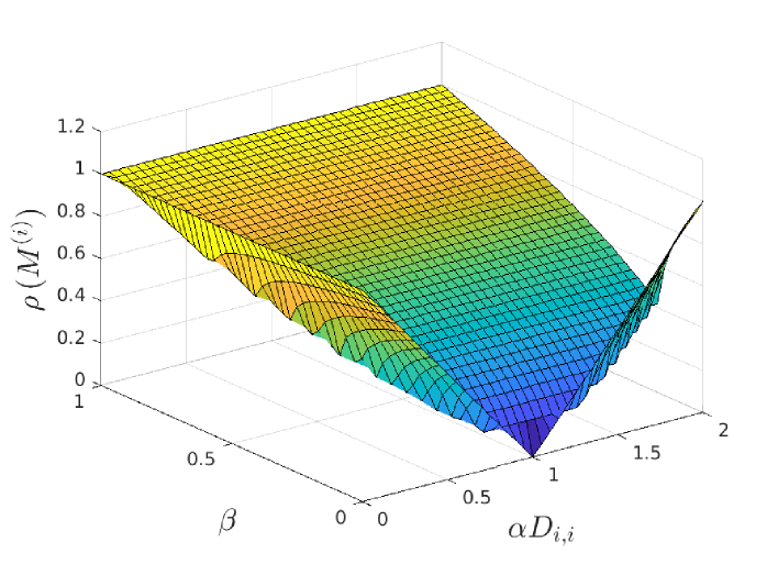
Figure 2: Spectral radius of $M^{(i)}$ as a function of $\alpha D_{i,i}\in(0,2]$ and $\beta\in[0,1)$.

In Figure 2, the value of $\alpha D_{i,i}\in(0,2]$ is plotted from the middle to the right and the value of $\beta$ from the middle to the rear-left. The associated values of $\rho$ are plotted on the vertical axis.

It is assumed that an upper bound $\overline{m}$ for the eigenvalues $D_{i,i}$ is known and that $\alpha$ is chosen less than or equal to $2/\overline{m}$ so that the possible values of $\alpha D_{i,i}$ vary over a (typically wide) range in the interval (0,2] and depend on the distribution of the eigenvalues. This range is problem dependent and not subject to the design of the method.

A fast convergence of the HBM (or of the momentum method MM) is obtained if the value of $\beta$ is chosen such that $\rho$ is small for a wide range of values $\alpha D_{i,i}$. Figure 2 gives the impression that this is achieved when choosing $\beta=0$. And indeed, when the values of $\alpha D_{i,i}$ all cluster about the value “1”, then the problem of minimizing $f$ not only is quite easy (since the condition number of $D$ is close to 1) but also choosing $\beta=0$ is nearly optimal.

However, when the condition number of $D$ is poor, then very small values of $\alpha D_{i,i}>0$ will occur. In this case, Figure 2 is not suitable for understanding the best possible choice of $\beta$. Instead, Figure 3 displays the plots of $\rho(M^{(i)})$ as a function of $\alpha D_{i,i}\in(0,2]$ for $\beta\equiv 0.9$ in red, $\beta\equiv 0.5$ in green, and $\beta\equiv 0.1$ in blue.

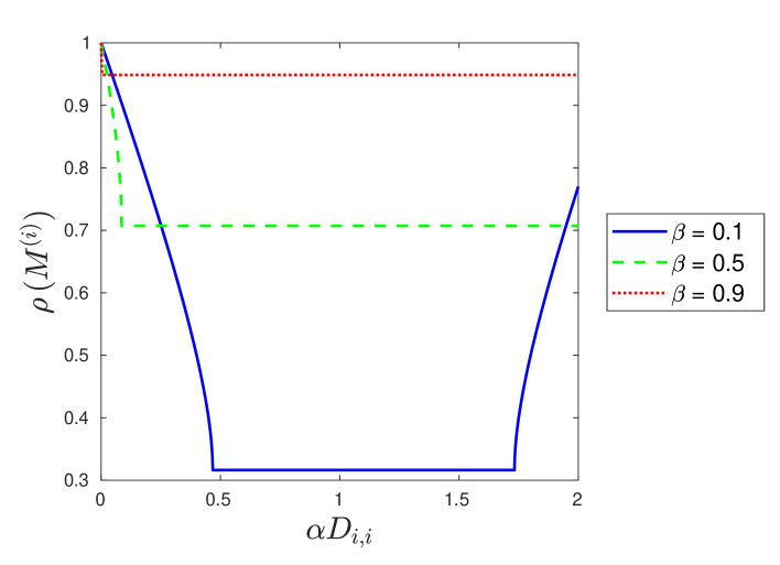
Figure 3: $\rho(M^{(i)})$ as a function of $\alpha D_{i,i}\in(0,2]$ for fixed values of $\beta$.

In Figure 3 the choice $\beta=0.1$ in blue leads to small values of $\rho(M^{(i)})$ when $\alpha D_{i,i}\in[0.5,1.5]$ (and a little beyond this interval). For values $\alpha D_{i,i}\approx 0.2$, the choice $\beta=0.5$ in green results in a much smaller value of $\rho(M^{(i)})$ than $\beta=0.1$, and as displayed in Figure 4, when considering poorly conditioned problems with some values of $\alpha D_{i,i}\approx 0.004$ the choice of $\beta=0.9$ in red results in a smaller value of $\rho(M^{(i)})$ than $\beta=0.5$ or $\beta=0.1$. (Figure 4 is a zoom of Figure 3; of course, small values of $\alpha D_{i,i}$ occurring in ill-conditioned problems result in an increase of $\rho(M^{(i)})$ but for small $\alpha D_{i,i}>0$ the increase is much less for larger values of $\beta<1$.)

An interesting observation that can be deduced from Figure 3 is the following: Recall that a step length $\alpha D_{i,i}>2$ is “too long” in the sense that it results in a divergent algorithm for the plain steepest descent method. For larger values of $\beta\geq 0.5$, however, the green line and the red line seem to (and do) continue “for a little while” with constant values to the right of $\alpha D_{i,i}=2$ which implies that for larger values of $\beta$ a step length that is a little bit “too long” still results in a convergent algorithm. In contrast to the intuition that with the use of momentum the step length needs to be chosen more carefully, actually the opposite is true.

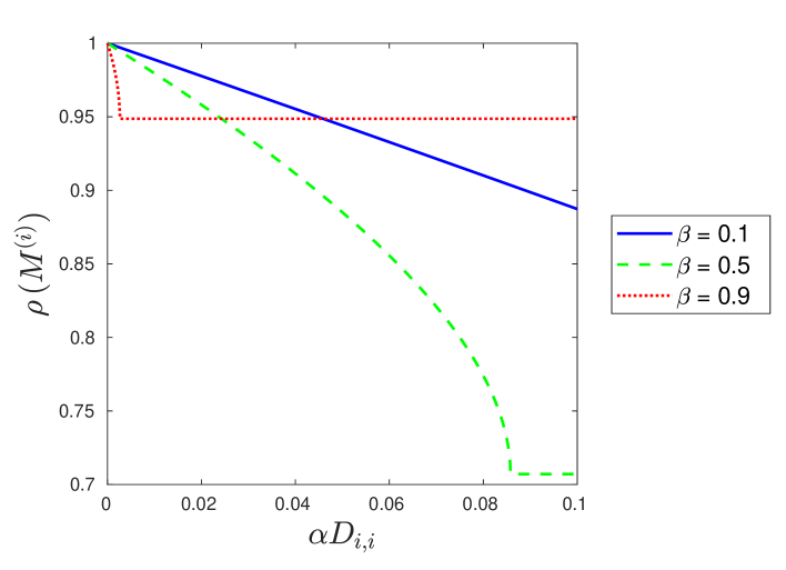
Figure 4: $\rho(M^{(i)})$ as a function of $\alpha D_{i,i}\in(0,0.1)$ for fixed values of $\beta$.

2.2 Selecting $\alpha$ and $\beta$

In the following it is assumed that a lower bound

$$0<\underline{m}\leq\min_{1\leq i\leq n}D_{i,i}\qquad\hbox{and an upper bound}\qquad\overline{m}\geq\max_{1\leq i\leq n}D_{i,i}$$

are known. Given $\overline{m}$, the step length $\alpha$ is fixed to

$$\alpha:=2/\overline{m}.$$ (7)

In the following let

$$\overline{\hbox{\rm con}}\hbox{\rm d}(D)\ \ :=\ \ \overline{m}/\underline{m}\ \ \geq\ \ \hbox{\rm cond}(D)$$

be an upper bound for $\hbox{\rm cond}(D)$. Often, an upper bound for $\overline{m}$ can be obtained, for example by Gershgorin’s theorem, while it may be difficult to determine a positive lower bound for $\underline{m}$. (The numerical effects of overestimating or underestimating the condition number of $H$ are analyzed in [5] along with an approach to adaptively adjust the estimate of the condition number, provided that function evaluations are available – an assumption that unfortunately is not satisfied in many stochastic settings.)

To simplify the discussion below, it is further assumed that

$$\overline{\hbox{\rm con}}\hbox{\rm d}(D)>2.$$ (8)

(In Theorem 1 a stronger restriction on $\overline{\hbox{\rm con}}\hbox{\rm d}(D)$ is made; for now (8) is sufficient. For well-conditioned problems with $\overline{\hbox{\rm con}}\hbox{\rm d}(D)\leq 2$ the plain steepest descent method with $\beta=0$ is optimal up to a factor of at most 2.)

When $\beta<3-2\sqrt{2}\approx 0.1716$ then there are two values of $\alpha D_{i,i}$ for which $(1+\beta-\alpha D_{i,i})^{2}=4\beta$ (corresponding, for example, to the end points of the blue horizontal line in Figure 3). The considerations below apply to values

$$\beta\geq 3-2\sqrt{2}$$

which have proved to be efficient in numerical experiments, see, for example, [16], and where only the left end point of the interval with constant values $\rho$ (i.e. of the horizontal lines in Figure 3) is relevant.

Let $\underline{\alpha}=\alpha\underline{m}$ be a lower bound for possible values of $\alpha D_{i,i}$. Assumption (8) implies $\underline{\alpha}<1$. Setting $\beta:=(1-\sqrt{\underline{\alpha}})^{2}$, the spectral radius of all $M^{(i)}$ (and thus, $\rho(M)$)) is upper bounded by $\sqrt{\beta}=1-\sqrt{\underline{\alpha}}$, i.e.

$$\rho(M)\leq\sqrt{\beta}=1-\sqrt{\underline{\alpha}}=1-\frac{\sqrt{2}}{\sqrt{\overline{\hbox{\rm con}}\hbox{\rm d}(D)}}.$$

When $\overline{\hbox{\rm con}}\hbox{\rm d}(D)$ approximates $\hbox{\rm cond}(D)$ up to a constant factor (this is what is meant with “appropriate” bound in the abstract of this paper) then the resulting order $1-\frac{1}{O(\sqrt{\hbox{\rm cond}(D)})}$ is the same order as the optimal rate of convergence of the conjugate gradient method, see e.g. [12]. Moreover, the $2\times 2$ transformation matrices transforming $M^{(i)}$ to diagonal form or, more generally, to the Jordan canonical form are independent of the dimension, so that the 2-norm of the transformation matrices that transform $\hat{M}$ to a canonical form also is independent of $n$.
However, the optimal bound for the conjugate gradient iterations applies to the $D$-norm, $\|z\|_{D}=\sqrt{z^{T}Dz}$, while the above rate applies to a transformed problem, and the transformation matrix may be very ill-conditioned. This is studied further in Section 2.3 below.

2.3 On the norm of the transformation matrices

Consider the case in (5) that $\gamma_{i}=\sqrt{\beta_{i}^{2}-4\beta}$ is nonzero. Then $v_{+}\not=v_{-}$ and $M^{(i)}$ is diagonalizable, i.e. $M^{(i)}=S\Lambda S^{-1}$ where $\Lambda$ is the diagonal matrix with the eigenvalues $\lambda_{\pm}=\tfrac{1}{2}(\beta_{i}\pm\gamma_{i})$ of (5) and $S:=S^{(i)}:=\begin{pmatrix}1&1\\ \lambda_{+}&\lambda_{-}\end{pmatrix}$ with columns $v_{\pm}$ as defined in (5).

There are two cases: Either $\gamma_{i}>0$ is real or $\gamma_{i}$ is purely imaginary.

If $\gamma_{i}>0$ is real then $\lambda_{+}\lambda_{-}=\tfrac{1}{4}(\beta_{i}^{2}-\gamma_{i}^{2})=\tfrac{1}{4}(\beta_{i}^{2}-(\beta_{i}^{2}-4\beta))=\beta$ and

$$S^{T}S=\begin{pmatrix}1+\tfrac{1}{4}(\beta_{i}+\gamma_{i})^{2}&1+\beta\\ 1+\beta&1+\tfrac{1}{4}(\beta_{i}-\gamma_{i})^{2}\end{pmatrix}.$$

Denote the eigenvalues of $S^{T}S$ by $\mu_{+}\geq\mu_{-}>0$. Then

$$\mu_{\pm}=1+\tfrac{1}{4}(\beta_{i}^{2}+\gamma_{i}^{2})\pm\tfrac{1}{2}\sqrt{\beta_{i}^{2}\gamma_{i}^{2}+4(1+\beta)^{2}}.$$ (9)

If $\gamma_{i}$ is purely imaginary and $S^{H}$ denotes the complex conjugate transpose of $S$, then

$$S^{H}S=\begin{pmatrix}1+|\lambda_{+}|^{2}&1+\bar{\lambda}_{+}\lambda_{-}\\[4.0pt] 1+\lambda_{+}\bar{\lambda}_{-}&1+|\lambda_{-}|^{2}\end{pmatrix}.$$

Using the definitions of $\lambda_{\pm}$ and $\gamma_{i}$ it follows $\lambda_{+}\bar{\lambda}_{-}=\lambda_{+}^{2}$ and $|\lambda_{+}|^{2}=|\lambda_{-}|^{2}=\beta$, and $S^{H}S$ is given by $S^{H}S=\begin{pmatrix}1+\beta&1+\lambda_{-}^{2}\\ 1+\lambda_{+}^{2}&1+\beta\end{pmatrix}$ with the eigenvalues

$$\mu_{\pm}=1+\beta\pm|1+\lambda_{+}^{2}|.$$ (10)

In both cases the condition number of $S$ is $\hbox{\rm cond}(S)=\sqrt{\mu_{+}/\mu_{-}}$ with $\mu_{\pm}$ defined in (9) or (10).

Let $\Lambda$ denote the diagonal matrix with diagonal entries $\lambda_{+}$ and $\lambda_{-}$. As $\lambda_{+}$ and $\lambda_{-}$ approach each other, i.e. as $\gamma_{i}\to 0$, the columns of $S=S^{(i)}$ become nearly linearly dependent and $\hbox{\rm cond}(S)$ tends to infinity. This observation is illustrated in Figure 5, and it implies that the argument

$$\|(M^{(i)})^{k}\|_{2}=\|S\Lambda^{k}S^{-1}\|_{2}\leq\|S\|_{2}\|\Lambda^{k}\|_{2}\|S^{-1}\|_{2}=\hbox{\rm cond}(S)\|\Lambda\|_{2}^{k}$$ (11)

for the convergence of $(M^{(i)})^{k}\to 0$ as $k\to\infty$ needs to be refined when $D$ has (small) positive eigenvalues for which $\gamma_{i}\approx 0$. Components $i$ for which $\gamma_{i}\approx 0$ will be called

critical components

below. Given the choice $\beta=(1-\sqrt{\underline{\alpha}})^{2}$, critical components are those with $D_{i,i}$ close to $\underline{m}$.

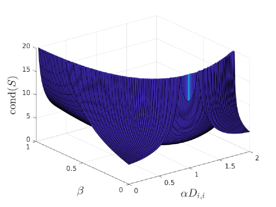
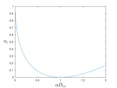
Figure 5: $\min\{\hbox{\rm cond}(S^{(i)}),\,20\}$ as a function of $\alpha D_{i,i}\in(0,2]$ and $\beta\in[0,1)$ on the left, and zeros of the terms $\gamma_{i}$ depending on $\alpha D_{i,i}$ and $\beta$ on the right plot.

2.4 The Schur canonical form

It turns out that the case $\gamma_{i}\approx 0$ can be analyzed by using the Schur-decomposition of $M^{(i)}$ with an upper right triangular matrix $R$ and a transformation matrix $T$ given by

$$TRT^{-1}:=\begin{pmatrix}1&0\\ \lambda_{+}&1\end{pmatrix}\begin{pmatrix}\lambda_{+}&1\\ 0&\lambda_{-}\end{pmatrix}\begin{pmatrix}1&0\\ -\lambda_{+}&1\end{pmatrix}=\begin{pmatrix}0&1\\ -\lambda_{+}\lambda_{-}&\lambda_{+}+\lambda_{-}\end{pmatrix}=\begin{pmatrix}0&1\\ -\beta&\beta_{i}\end{pmatrix}=M^{(i)}.$$

Note that this decomposition is valid for both cases: for $\gamma_{i}=0$ as well as for $\gamma_{i}\neq 0$. (When $\gamma_{i}=0$ i.e. when $\lambda_{+}=\lambda_{-}$ this is the Jordan canonical form.)

Now, in place of (11), also the argument

$$\|(M^{(i)})^{k}\|=\|(TRT^{-1})^{k}\|=\|TR^{k}T^{-1}\|\leq\|T\|\cdot\|T^{-1}\|\cdot\|R^{k}\|=\hbox{\rm cond}(T)\cdot\|R^{k}\|$$ (12)

can be used. While both (11) and (12) lead to valid bounds for $\|(M^{(i)})^{k}\|$ whenever (11) is defined and thus, the better of both bounds can be used, the estimate below relies on (12) which is always well defined. Bounds on $\hbox{\rm cond}(T)$ and on $\|R^{k}\|$ are derived next:

By Gershgorin’s theorem, given a triangular matrix

$$\hat{R}=\begin{pmatrix}a&b\\ 0&c\end{pmatrix}$$

with complex numbers $a,b,c$ and $|a|\geq|c|$, the 2-norm of $\hat{R}$ is bounded by

$$\|\hat{R}\|_{2}=\lambda_{max}\left(\begin{pmatrix}\bar{a}&0\\ \bar{b}&\bar{c}\end{pmatrix}\begin{pmatrix}a&b\\ 0&c\end{pmatrix}\right)^{1/2}\!\!=\lambda_{max}\left(\begin{pmatrix}|a|^{2}&\bar{a}b\\ a\bar{b}&|c|^{2}+|b|^{2}\end{pmatrix}\right)^{1/2}\leq\sqrt{|a|^{2}+|ab|+|b|^{2}}$$ (13)

(with $\lambda_{max}$ denoting the maximum eigenvalue).

Since $\|\hat{R}\|_{2}=\|\hat{R}^{H}\|_{2}$ the bound (13) also applies to the matrix $T$ and yields

$$\|T\|_{2}^{2}\leq 1+|\lambda_{+}|+|\lambda_{+}|^{2}\leq 3$$ (14)

since $|\lambda_{+}|\leq\rho(M^{(i)})<1$. The same estimate applies to $\|T^{-1}\|_{2}^{2}$, so that $\hbox{\rm cond}(T)\leq 3$.

Inductively, it can be verified that the $k^{\text{th}}$ power of the matrix $R$ is given by

$$R^{k}=\begin{pmatrix}\lambda_{+}^{k}&\sum_{\ell=0}^{k-1}\lambda_{+}^{\ell}\lambda_{-}^{k-1-\ell}\\ 0&\lambda_{-}^{k}\end{pmatrix}.$$

By definition $|\lambda_{+}|\leq\rho$ and $|\lambda_{-}|\leq\rho$ apply. (If $\gamma_{i}=0$, then actually $\rho=|\lambda_{-}|=|\lambda_{+}|$ — and this is the “worst case” in the estimate below). In any case, it follows with the triangle inequality that the absolute value of the upper right entry of $R^{k}$ is bounded by $|(R^{k})_{1,2}|\leq k\rho^{k-1}$, and then, by (13), that

$$\|R^{k}\|\leq\rho^{k-1}\sqrt{\rho^{2}+k\rho+k^{2}}\leq\rho^{k-1}\sqrt{1+k+k^{2}}\leq\rho^{k-1}(k+1).$$ (15)

Since the condition number of $T$ is at most 3, the norm $\|(M^{(i)})^{k}\|$ is at least $\frac{1}{3}\|R^{k}\|$ and at most $3\|R^{k}\|$. The latter observation can be used to bound the number of iterations needed to reduce the (unknown) Euclidean distance of a given point $x^{0}$ to the optimal solution by a factor $\epsilon>0$. This is done in the next section with a slightly tighter bound of $\|(M^{(i)})^{k}\|$.

2.5 On the rate of convergence

Inserting (14) and (15) in (12) yields $\|(M^{(i)})^{k}\|_{2}\leq 3\rho^{k-1}(k+1)$. This bound is based on the sub-multiplicativity of the 2-norm. When computing $(M^{(i)})^{k}$ explicitly, it can be reduced to

$$\|(M^{(i)})^{k}\|_{2}\leq 2\rho^{k-1}(k+1).$$ (16)

The somewhat tedious calculations leading to (16) are given in the Appendix. Let a desired accuracy $\epsilon\in(0,1)$ be given. To obtain a sufficient condition for

$$2\rho^{k-1}(k+1)\leq\epsilon\ \ \Longleftrightarrow\ \ (k\!-\!1)\ln(\rho)+\ln(k+1)\leq\ln(\tfrac{\epsilon}{2})$$ (17)

the bound $\ln(\rho)\leq\rho-1$ is used,

$$(\ref{boundk})\ \ \Longleftarrow \ \ (k\!-\!1)(\rho-1)+\ln(k+1)\leq\ln(\tfrac{\epsilon}{2})$$ (18)

$$\Longleftrightarrow \ \ (1-\rho)(k\!-\!1)\geq\ln(\tfrac{2}{\epsilon})+\ln(k+1)$$

Denote

$$\delta:=\tfrac{1}{\sqrt{2\ \overline{\hbox{\rm con}}\hbox{\rm d}(D)}}=\tfrac{1-\sqrt{\beta}}{2}\leq\tfrac{1-\rho}{2}.$$

If the following two inequalities are satisfied then (18) is satisfied as well,

$$\delta(k-1)\geq\ln(\tfrac{2}{\epsilon})\qquad\hbox{and}\qquad\delta(k-1)\geq\ln(k+1).$$ (19)

Here $\delta>0$ depends on $\beta=(1-\sqrt{\underline{\alpha}})^{2}$, i.e. on the choice of the parameters $\alpha,\beta$ that in turn depend on the bounds $\underline{m}$ and $\overline{m}$ of the eigenvalues of $D$. Below it is assumed that $\delta\leq\exp(-2)$ – which is the case when $\overline{\hbox{\rm con}}\hbox{\rm d}(D)\geq 28$.

Then, the second relation in (19) is satisfied whenever $k\geq\bar{k}:=\frac{2}{\delta}\ln(\frac{1}{\delta})-1$.

Indeed,

$$\delta(\bar{k}-1)-\ln(\bar{k}+1) = 2\ln(\tfrac{1}{\delta})-2\delta-\ln(\tfrac{2}{\delta}\ln(\tfrac{1}{\delta}))$$

$$= \ln(\tfrac{1}{\delta})-2\delta-\ln(\ln(\tfrac{1}{\delta}))-\ln(2)$$

$$> 0$$

for $0<\delta\leq\exp(-2)$.

Thus it suffices to ensure that the first inequality in (19) implies the second. This is the case when $\epsilon$ is sufficiently small: Indeed, the first bound in (19) is satisfied for $k=\bar{k}$ with equality if

$$\epsilon=\bar{\epsilon}:=2\delta^{2}e^{2\delta}.$$

For $\epsilon\leq\bar{\epsilon}$ all values of $k$ satisfying the first relation in (19) are greater or equal to $\bar{k}$ so that the second relation is satisfied as well. Since $e^{2\delta}>1$ it is sufficient to choose $\epsilon\leq 2\delta^{2}=1\,/\overline{\hbox{\rm con}}\hbox{\rm d}(D)$. The first relation in (19) can be written as

$$k\geq\ln\left(\tfrac{2}{\epsilon}\right)\cdot\tfrac{1}{\delta}+1=\ln\left(\tfrac{2}{\epsilon}\right)\cdot\sqrt{2\ \overline{\hbox{\rm con}}\hbox{\rm d}(D)}+1.$$ (20)

Thus, when $k$ satisfies (20) with $\epsilon\leq 2\delta^{2}$, relation (17) is satisfied and

$$\sqrt{2}\|\tfrac{1}{2}(x^{k-1}+x^{k})\|_{2}=\left\|\tfrac{1}{2}\left(\left(\begin{matrix}x^{k-1}\\ x^{k}\end{matrix}\right)+\left(\begin{matrix}x^{k}\\ x^{k-1}\end{matrix}\right)\right)\right\|_{2}\leq\tfrac{1}{2}\left(\left\|\left(\begin{matrix}x^{k-1}\\ x^{k}\end{matrix}\right)\right\|_{2}+\left\|\left(\begin{matrix}x^{k}\\ x^{k-1}\end{matrix}\right)\right\|_{2}\right)$$

$$= \tfrac{1}{2}\left(\left\|\left(\begin{matrix}x^{k-1}\\ x^{k}\end{matrix}\right)\right\|_{2}+\left\|\left(\begin{matrix}x^{k-1}\\ x^{k}\end{matrix}\right)\right\|_{2}\right)=\left\|\left(\begin{matrix}x^{k-1}\\ x^{k}\end{matrix}\right)\right\|_{2}\leq\epsilon\left\|\left(\begin{matrix}x^{0}\\ x^{1}\end{matrix}\right)\right\|_{2}\leq\sqrt{2}\epsilon\|x^{0}\|_{2}$$

where the last inequality follows from $\|x^{1}\|_{2}\leq\|x^{0}\|_{2}$, the first step being a plain steepest descent step with step length $2/\overline{m}$. Summarizing, the claim of Theorem 1 follows. $\square$

2.6 Nesterov’s accelerated gradient method

For the analysis of Nesterov’s accelerated gradient method again it suffices to consider the function $f$ in (2) with $\nabla f(x)=Dx$. Replacing $(HBM)$ with $(NAG)$ in the form (1) it follows that the matrix $M^{(i)}=\left(\begin{matrix}0&&1\\ -\beta&&\beta_{i}\end{matrix}\right)$ in (4) is to be replaced with

$$M^{(i)}:=\left(\begin{matrix}0&&1\\ -\beta(1-\alpha_{i})&&(1+\beta)(1-\alpha_{i})\end{matrix}\right)$$

where again, $\alpha_{i}:=\alpha D_{i,i}$. Thus, replacing $\beta$ and $\beta_{i}$ in (4) with $\beta(1-\alpha_{i})$ and $(1+\beta)(1-\alpha_{i})$ it follows that $\rho$ in (6) changes to

$$\rho:=\rho(M^{(i)})=\left\{\begin{array}[]{ll}\sqrt{\beta(1-\alpha_{i})}&\hbox{if}\ \ (1+\beta)^{2}(1-\alpha_{i})^{2}\leq 4\beta(1-\alpha_{i})\\[4.0pt] \frac{1}{2}\left(|(1+\beta)(1-\alpha_{i})|+\bar{\gamma}_{i}\right)&\hbox{else}\end{array}\right.$$ (21)

where $\bar{\gamma}_{i}:=\sqrt{(1+\beta)^{2}(1-\alpha_{i})^{2}-4\beta(1-\alpha_{i})}$. The first case of definition (21) can only be obtained for $\alpha_{i}\leq 1$. This results in half the step length $\alpha:=\frac{1}{\overline{m}}$ compared to (7) for $(HBM)$ and it then follows for $\alpha_{i}\in[1/\overline{\hbox{\rm con}}\hbox{\rm d}(D),1]$ and $\beta:=\tfrac{\left(\sqrt{\overline{\hbox{\rm con}}\hbox{\rm d}(D)}-1\right)^{2}}{\overline{\hbox{\rm con}}\hbox{\rm d}(D)-1}$ that $(1+\beta)^{2}(1-\alpha_{i})\leq 4\beta$ and

$$\rho=\sqrt{\beta(1-\alpha_{i})}\leq 1-\tfrac{1}{\sqrt{\overline{\hbox{\rm con}}\hbox{\rm d}(D)}}.$$

This is the same bound as for the $(MM)$ when taking half the step length $\alpha$ or – which is the same – when replacing $\overline{m}$ in $(MM)$ with $2\overline{m}$. In contrast to the $(MM)$, however, based on this analysis a theoretical justification of a longer step length $\alpha>1/\overline{m}$ is not possible.
The eigenvalues of $M^{(i)}$ are now given by

$$\lambda_{\pm}=\tfrac{1}{2}(\ (1+\beta)(1-\alpha_{i})\pm\sqrt{(1+\beta)^{2}(1-\alpha_{i})^{2}-4\beta(1-\alpha_{i})}\ )$$

and with this definition the matrix $T$ transforming $M^{(i)}$ to the Schur canonical form is the same as in Section 2.4. The iteration complexity for $(MM)$ thus applies to $(NAG)$ as well when replacing $\overline{\hbox{\rm con}}\hbox{\rm d}(D)$ with $2\,\overline{\hbox{\rm con}}\hbox{\rm d}(D)$. Summarizing, the following result is obtained:

Theorem 2

Let $f:{\mathbb{R}}^{n}\to{\mathbb{R}}$ be a strictly convex quadratic function with minimizer $x^{*}$ and denote $H:=\nabla^{2}f(x^{*})$. Let $\overline{m}$ be an upper bound for the eigenvalues of $H$ and let $0<\underline{m}$ be a lower bound for the eigenvalues of $H$. Then $\overline{\hbox{\rm con}}\hbox{\rm d}(H):=\overline{m}/\underline{m}$ is an upper bound for the condition number of $H$. Assume that $\overline{\hbox{\rm con}}\hbox{\rm d}(H)\geq 28$.
In $(HBM)$ define $\alpha=1/\overline{m}$,  $\underline{\alpha}=1/\overline{\hbox{\rm con}}\hbox{\rm d}(H)$,  $\beta=\tfrac{\left(1-\sqrt{\underline{\alpha}}\right)^{2}}{1-\underline{\alpha}}$ and let $\epsilon\leq 1\,/\,\overline{\hbox{\rm con}}\hbox{\rm d}(H)$ be given. Then, given $x^{0}\in{\mathbb{R}}^{n}$, after

$$1+\lceil 2\,\sqrt{\overline{\hbox{\rm con}}\hbox{\rm d}(H)}\ \ln(\tfrac{2}{\epsilon})\rceil$$

steps of the $(NAG)$, an approximate solution $\bar{x}^{k}:=\tfrac{1}{2}(x^{k-1}+x^{k})$ is generated with

$$\|\bar{x}^{k}-x^{*}\|_{2}\leq\epsilon\|x^{0}-x^{*}\|_{2}.$$

2.7 A note on the rate of convergence

Theorem 1 and Theorem 2 address the iteration complexity with respect to the Euclidean norm while the asymptotic rate of convergence of $(NAG)$ or $(HBM)$ (with respect to any fixed norm) is given by the maximum spectral radius of all matrices $M^{(i)}$ which coincides with the value $1-\sqrt{\underline{\alpha}}$ under the assumptions of Theorems 1 and 2. Thus, the asymptotic rate of convergence is

• $1-\sqrt{1/\overline{\hbox{\rm con}}\hbox{\rm d}(H)}$ for $(NAG)$ and

• $1-\sqrt{2/\overline{\hbox{\rm con}}\hbox{\rm d}(H)}$ for $(HBM)$.

Here, the rate for $(HBM)$ is somewhat worse than the asymptotic rate $1-2/\sqrt{\overline{\hbox{\rm con}}\hbox{\rm d}(H)}$ for $(HBM)$ established in [15], Theorem 9 (3), the difference being due to the limitation of the step length $\alpha$ which is nearly twice as long in [15] as considered here – and four times as long as for Nesterov’s accelerated gradient method.

The rates of convergence are not just upper bounds but exact rates once the values $\underline{m}$ and $\overline{m}$ are given, and hence, the difference in the rates of convergence for $(NAG)$ and $(HBM)$ can be explained just by the limitations of the step length: when the $(HBM)$ is restricted to steps $\alpha=1/\overline{m}$ as for $(NAG)$, its asymptotic rate of convergence is exactly the same as $(NAG)$.

The above rate for Nesterov’s accelerated gradient method is the same as established for the convergence of the function values in [14], Theorem 2.2.3. Translated to the error measure $\|x-x^{*}\|_{H}=\sqrt{f(x)-f(x^{*})}$ the rate of convergence of [14], Theorem 2.2.3 reduces to approximately $1-\sqrt{1/2\,\overline{\hbox{\rm con}}\hbox{\rm d}(H)}$.

3. Conclusion

The asymptotic rate of convergence of the momentum method for fixed parameters has been analyzed in the classical work [15]. Here, the constants in this work are considered and an explicit bound for the iteration complexity is derived that also applies in slightly modified form to Nesterov’s accelerated gradient method.

Acknowledgment

The authors would like to thank Robert Gower for helpful e-mail-discussions.

Appendix

The matrix $M^{i,k}:=(M^{(i)})^{k}$ can also be written as

$$(M^{(i)})^{k} =TR^{k}T^{-1}=\begin{pmatrix}1&0\\ \lambda_{+}&1\end{pmatrix}\begin{pmatrix}\lambda_{+}^{k}&\ \ \ \sum_{\ell=0}^{k-1}\lambda_{+}^{\ell}\lambda_{-}^{k-1-\ell}\\[4.0pt] 0&\lambda_{-}^{k}\end{pmatrix}\begin{pmatrix}1&0\\ -\lambda_{+}&1\end{pmatrix}$$

$$=\begin{pmatrix}1&0\\ \lambda_{+}&1\end{pmatrix}\begin{pmatrix}\lambda_{+}^{k}-\lambda_{+}\sum_{\ell=0}^{k-1}\lambda_{+}^{\ell}\lambda_{-}^{k-1-\ell}&\ \ \ \ \ \sum_{\ell=0}^{k-1}\lambda_{+}^{\ell}\lambda_{-}^{k-1-\ell}\\[4.0pt] -\lambda_{+}\lambda_{-}^{k}&\lambda_{-}^{k}\end{pmatrix}$$

$$=\begin{pmatrix}\lambda_{+}^{k}-\lambda_{+}\sum_{\ell=0}^{k-1}\lambda_{+}^{\ell}\lambda_{-}^{k-1-\ell}&\sum_{\ell=0}^{k-1}\lambda_{+}^{\ell}\lambda_{-}^{k-1-\ell}\\[4.0pt] \lambda_{+}^{k+1}-\lambda_{+}^{2}\sum_{\ell=0}^{k-1}\lambda_{+}^{\ell}\lambda_{-}^{k-1-\ell}-\lambda_{+}\lambda_{-}^{k}&\ \ \ \ \ \lambda_{+}\sum_{\ell=0}^{k-1}\lambda_{+}^{\ell}\lambda_{-}^{k-1-\ell}+\lambda_{-}^{k}\end{pmatrix}$$

$$=\begin{pmatrix}\lambda_{+}^{k}-\sum_{\ell=0}^{k-1}\lambda_{+}^{\ell+1}\lambda_{-}^{k-1-\ell}&\sum_{\ell=0}^{k-1}\lambda_{+}^{\ell}\lambda_{-}^{k-1-\ell}\\[4.0pt] \lambda_{+}^{k+1}-\sum_{\ell=0}^{k-1}\lambda_{+}^{\ell+2}\lambda_{-}^{k-1-\ell}-\lambda_{+}\lambda_{-}^{k}&\ \ \ \ \ \sum_{\ell=0}^{k-1}\lambda_{+}^{\ell+1}\lambda_{-}^{k-1-\ell}+\lambda_{-}^{k}\end{pmatrix}$$

$$=\begin{pmatrix}-\sum_{\ell=0}^{k-2}\lambda_{+}^{\ell+1}\lambda_{-}^{k-1-\ell}&\sum_{\ell=0}^{k-1}\lambda_{+}^{\ell}\lambda_{-}^{k-1-\ell}\\[4.0pt] -\sum_{\ell=-1}^{k-2}\lambda_{+}^{\ell+2}\lambda_{-}^{k-1-\ell}&\ \ \ \sum_{\ell=-1}^{k-1}\lambda_{+}^{\ell+1}\lambda_{-}^{k-1-\ell}\end{pmatrix}$$

$$=\begin{pmatrix}-\sum_{t=1}^{k-1}\lambda_{+}^{t}\lambda_{-}^{k-t}&\ \ \sum_{\ell=0}^{k-1}\lambda_{+}^{\ell}\lambda_{-}^{k-1-\ell}\\[4.0pt] -\sum_{t=0}^{k-1}\lambda_{+}^{t+1}\lambda_{-}^{k-t}&\sum_{t=0}^{k}\lambda_{+}^{t}\lambda_{-}^{k-t}\end{pmatrix}=:\begin{pmatrix}p&q\\ r&s\end{pmatrix}\in\mathbb{R}^{2\times 2},$$

where in the last row the index shift $t:=\ell+1$ was used. (The definition of the real numbers $p,q,r,s$ depends on the possibly complex eigenvalues $\lambda_{+}$ and $\lambda_{-}$.)

The matrix product $(M^{i,k})^{\text{T}}M^{i,k}$ is

$$(M^{i,k})^{\text{T}}M^{i,k}=\begin{pmatrix}p&r\\ q&s\end{pmatrix}\begin{pmatrix}p&q\\ r&s\end{pmatrix}=\begin{pmatrix}p^{2}+r^{2}&pq+rs\\ pq+rs&q^{2}+s^{2}\end{pmatrix}=\begin{pmatrix}a&b\\ b&d\end{pmatrix}$$

with

$$a :=p^{2}+r^{2}=\left(\sum_{\ell=1}^{k-1}\lambda_{+}^{\ell}\lambda_{-}^{k-\ell}\right)^{2}+\left(\sum_{\ell=0}^{k-1}\lambda_{+}^{\ell+1}\lambda_{-}^{k-\ell}\right)^{2},$$

$$b :=pq+rs=-\left(\sum_{\ell=1}^{k-1}\lambda_{+}^{\ell}\lambda_{-}^{k-\ell}\right)\left(\sum_{\ell=0}^{k-1}\lambda_{+}^{\ell}\lambda_{-}^{k-1-\ell}\right)-\left(\sum_{\ell=0}^{k-1}\lambda_{+}^{\ell+1}\lambda_{-}^{k-\ell}\right)\left(\sum_{\ell=0}^{k}\lambda_{+}^{\ell}\lambda_{-}^{k-\ell}\right),$$

$$d :=q^{2}+s^{2}=\left(\sum_{\ell=0}^{k-1}\lambda_{+}^{\ell}\lambda_{-}^{k-1-\ell}\right)^{2}+\left(\sum_{\ell=0}^{k}\lambda_{+}^{\ell}\lambda_{-}^{k-\ell}\right)^{2}.$$

By definition of the spectral radius $\rho=\rho(M^{(i)})<1$ the inequalities $|\lambda_{+}|\leq\rho$ and $|\lambda_{-}|\leq\rho$ hold, and thus,

$$a\leq 2k^{2}\rho^{2k}\quad\hbox{and}\quad d\leq 2(k+1)^{2}\rho^{2k-2}.$$

Since $(M^{i,k})^{\text{T}}M^{i,k}\succeq 0$ the maximum eigenvalue of $(M^{i,k})^{\text{T}}M^{i,k}$ is at most equal to the trace, i.e.

$$\lambda_{\max}((M^{i,k})^{\text{T}}M^{i,k})\leq a+d\leq 4\rho^{2(k-1)}(k+1)^{2}.$$

This way, an upper bound for the norm of $M^{i,k}$ is given by

$$\|M^{i,k}\|_{2}\leq 2\rho^{k-1}(k+1).$$ (22)

To estimate in how far the above bound is tight, consider the case of $\gamma_{i}=0$, i. e. $\rho=|\lambda_{+}|=|\lambda_{-}|$. It then follows

$$a\geq 2(k-1)^{2}\rho^{2k+2},\qquad b\leq-2(k-1)^{2}\rho^{2k+1},\qquad d\geq 2(k-1)^{2}\rho^{2k}$$

and with $z:=(1,\ -1)^{T}$ that

$$\lambda_{\max}((M^{i,k})^{\text{T}}M^{i,k})\geq\tfrac{z^{T}(M^{i,k})^{\text{T}}M^{i,k}z}{z^{T}z}\geq\tfrac{8(k-1)^{2}\rho^{2k+2}}{2}.$$

Thus,

$$\|M^{i,k}\|_{2}\geq 2\rho^{k+1}(k-1),$$

i.e. up to the changes $k+1\longleftrightarrow k-1$ the bound (22) is sharp.

Again, the “critical components” i.e. those with $\gamma_{i}\approx 0$ lead to a poor convergence, i.e. to the case where (22) is almost sharp. On the other hand, $(M^{i,k})^{T}M^{i,k}$ is almost singular, and for a critical component $i$ the quantity $\alpha_{i}$ is small so that the iterates $x^{0}$ and $x^{1}$ of $(MM)$ with step length $2/\overline{m}$ satisfy $x^{0}_{i}\approx x^{1}_{i}$. This again implies that the vector $z_{(i)}^{1}:=(x^{0}_{i},\ x^{1}_{i})^{T}$ is close to the eigenvector of $(M^{i,k})^{T}M^{i,k}$ associated with the small eigenvalue, i.e.

$$\|M^{i,k}z_{(i)}^{1}\|_{2}^{2}=(z_{(i)}^{1})^{T}(M^{i,k})^{T}M^{i,k}z_{(i)}^{1}\ll\|M^{i,k}\|_{2}^{2}\|z_{(i)}^{1}\|_{2}^{2}.$$

References

- [1] Barré, M., Taylor, A., d’Aspremont, A. (2020): Complexity Guarantees for Polyak Steps with Momentum. 33rd Annual Conference on Learning Theory, Proceedings of Machine Learning Research, Vol. 125, 1-27.
- [2] Defazio, A. (2021): Momentum via Primal Averaging: Theoretical Insights and Learning Rate Schedules for Non-Convex Optimization. https://arxiv.org/pdf/2010.00406.pdf
- [3] Défossez, A., Bottou, L., Bach, F., Usunier, N. (2022): A Simple Convergence Proof of Adam and Adagrad. Transactions on Machine Learning Research. https://arxiv.org/pdf/2003.02395.pdf
- [4] Diakonioklas, J., Jordan, M.I. (2021): Generalized Momentum-Based Methods: a Hamiltonian Perspective. SIAM J.Optim. Vol. 31, No. 1, 915-944.
- [5] O’Donoghue, B., Candès. E. (2015): Adaptive Restart for Accelerated Gradient Schemes. Foundations of computational mathematics, Vol. 15, No 3, 715-732.
- [6] Ganesh, S., Deb, R., Thoppe, G., Budhiraja, A. (2022): Does Momentum Help in Stochastic Optimization? A Sample Complexity Analysis. https://arxiv.org/abs/2110.15547v3
- [7] Gitman, I., Lang, H., Zhang, P., Xiao, L. (2019): Understanding the Role of Momentum in Stochastic Gradient Methods. H. Wallach, H. Larochelle, A. Beygelzimer, F. d’Alché-Buc, E. Fox, R. Garnett (eds): Advances in Neural Information Processing Systems, 32 (NeurIPS 2019), https://proceedings.neurips.cc/paper/2019
- [8] Goh, G. (2017): Why Momentum Really Works. Distill, http://distill.pub/2017/momentum
- [9] Gratton, S., Jerad, S., Toint, Ph. L. (2022): First-Order Objective-Function-Free Optimization Algorithms and Their Complexity.
- [10] Gratton, S., Jerad, S., Toint, Ph. L. (2022): Parametric complexity analysis for a class of first-order Adagrad-like algorithms. https://arxiv.org/pdf/2203.01647.pdf
- [11] Gratton, S., Toint, Ph. L. (2022): OFFO minimization algorithms for second-order optimality and their complexity. https://arxiv.org/pdf/2203.03351.pdf
- [12] Li, R.C. (2008): On Meinardus’ examples for the conjugate gradient method, Mathematics of Computation, Vol. 77, Nr. 261, 335-352.
- [13] Nesterov, Y.E. (1983): A method for solving the convex programming problem with convergence rate . Dokl. akad. nauk Sssr 269, 543-547.
- [14] Nesterov, Y.E. (2003): Introductory lectures on convex optimization: A basic course. Springer Science and Business Media, Vol. 87.
- [15] Polyak, B.T. (1964): Some methods of speeding up the convergence of iteration methods. USSR Computational Mathematics and Mathematical Physics, 4(5):1-17.
- [16] Sebbouh, O., Gower, R.M., Defazio, A. (2020): On the convergence of the Stochastic Heavy Ball Method. https://othmanesebbouh.github.io/publications/heavyball.pdf
- [17] The GitHub repository: https://github.com/MHagedorn/momentum (2022)
- [18] Yang, T., Lin, Q., Li, Z. (2016): Unified Convergence Analysis of Stochastic Momentum Methods for Convex and Non-convex Optimization. https://arxiv.org/pdf/1604.03257.pdf