Convergence of Adapted Empirical Measures on $\mathbb{R}^{d}$

Abstract

We consider empirical measures of $\mathbb{R}^{d}$-valued stochastic process in finite discrete-time. We show that the adapted empirical measure introduced in the recent work [Bac+22] by Backhoff et al. in compact spaces can be defined analogously on $\mathbb{R}^{d}$, and that it converges almost surely to the underlying measure under the adapted Wasserstein distance. Moreover, we quantitatively analyze the convergence of the adapted Wasserstein distance between those two measures. We establish convergence rates of the expected error as well as the deviation error under different moment conditions. Under suitable integrability and kernel assumptions, we recover the optimal convergence rates of both expected error and deviation error. Furthermore, we propose a modification of the adapted empirical measure with projection on a non-uniform grid, which obtains the same convergence rate but under weaker assumptions.

Keywords: adapted Wasserstein distance, empirical measure, convergence rate
MSC (2020): 60B10, 62G30, 49Q22

1 Introduction

Empirical measures analysis addresses the fundamental question of how well empirical observations approximate the underlying distribution. The quality of the approximation is measured by how close the empirical value approximates the true value that we are interested in (e.g. expected utility). Precisely stated, it studies the convergence in functional values under the empirical measure to the ones under the true, underlying measure. For many problems, the functional is of the form $\int f(x)\mu(dx)$, where $f$ is a real-valued continuous function and $\mu$ is a probability measure. Under mild integrability assumptions, such functional is continuous with respect to the Wasserstein distance, an important metric intensively studied in statistics theories [FG15] as well as adopted in machine learning applications [AL18]. Therefore, the convergence of empirical measures is classically studied under Wasserstein distance. However, in stochastic finance, many important problems such as pricing and hedging problems, optimal stopping problems, and utility maximization problems, are actually not continuous with respect to Wasserstein distance. To wit, two stochastic models can be arbitrarily close to each other under Wasserstein distance, while the values of the mentioned optimization problems under the two models can be quite far from each other.

These problems, as well as many other stochastic optimization problems in a dynamic framework, are instead Lipschitz continuous with respect to a more strict distance, called adapted Wasserstein distance, which takes the temporal structure of stochastic processes into account; see [Bac+20]. This Lipschitz property implies that the adapted Wasserstein distance is strong enough to guarantee the robustness of path-dependent problems. On the other hand, it is so strong that even the empirical measures do not converge to the corresponding underlying measure under it; see [PP16]. Intuitively speaking, this is because the empirical measure is so “singular” that it can not explain the conditional laws. A remedy to this undesirable effect is to modify the empirical measure, so that the new measure has a nontrivial temporal structure and that it converges under adapted Wasserstein distance. In this spirit, Pflug and Pichler in [PP16] deploy smoothing convolutions on paths and prove that the convoluted measures converge. Alternatively, Backhoff et al. in [Bac+22] project paths on a grid and prove that the empirical measures of the projected paths converge. Both works prove that modified measures converge under adapted Wasserstein distance, though they are both limited to the case when the underlying measure is compactly supported. This condition is not satisfied by many important models in stochastic finance, e.g. the discretized Black-Scholes model, the Autoregressive model, the Fama-French model, etc.

In the present paper, we drop the assumption of compactness, and investigate the case of general, finite discrete-time stochastic processes which take values on $\mathbb{R}^{d}$. We stress the importance of being able to deal with measures with unbounded support, as this is always the case for stochastic models used in finance and insurance applications and beyond. We define the adapted empirical measure on $\mathbb{R}^{dT}$ analogously to the one in [Bac+22], and establish convergence results under adapted Wasserstein distance.

The first main contribution of the present paper is the generalization of all convergence results in [Bac+22] beyond the compactly supported constraint. We first show that adapted empirical measures converge under adapted Wasserstein distance almost surely as long as the underlying measure is integrable. Then, we compute the convergence rates of the expected error as well as of the deviation error under the uniform finite moment condition and the uniform Lipschitz kernel assumption. Under the finite moment condition, we prove polynomial convergence rates of the expected error as well as of the deviation error depending on the order of the finite moment. In particular, if the underlying measure $\mu\in\mathcal{P}(\mathbb{R}^{dT})$ satisfies $p$-th moment conditions with $p>\frac{d}{d-1}$, we recover the optimal rates of the expected error, which are known for the classical empirical measure with respect to Wasserstein distance; see [FG15]. Under the exponential moment condition, we prove the sharp optimal convergence rates of the expected error as well as the deviation error. Indeed, this recovers the optimal expected error rates and exponential deviation rates in [Bac+22].

Another main contribution of the article is the introduction of the non-uniform adapted empirical measure. We define a non-uniform grid on $\mathbb{R}^{dT}$, which is denser around the origin and coarser at the distance. Then we project paths on this non-uniform grid and refer to the empirical measure of the projected paths as the non-uniform adapted empirical measure. We show that all convergence results mentioned above are valid for the non-uniform adapted empirical measure as well. Moreover, in this case we can obtain the same polynomial convergence rate of the expected error but under a milder moment assumption, independent of $T$ and decaying with the dimension $d$.

The results obtained in this paper are of relevance for the wide range of applications of the adapted empirical measures on $\mathbb{R}^{d}$. In statistical learning theory, our results generalize the consistency result of empirical Wasserstein correlation coefficient in [Wie22]. In machine learning, our results contribute a primal numerical scheme evaluating the adapted Wasserstein distance as for the discriminator of generative adversarial models in [Xu+20, Kle+22]. In mathematical finance, our results provide finite samples guarantee of distributionally robust evaluation, such as superhedging prices, expected risks, etc.; see [Han22, OW21].

Organization of the paper. We conclude the Introduction with a review of the related literature. Then, in Section 2, we introduce the uniform and the non-uniform adapted empirical measures and state our main convergence results. In Section 3 we provide lemmas which will be used in the proofs of the main results. In Section 4 we prove convergence rates of the expected error. In Section 5 we prove polynomial convergence rates of the deviation error under finite moment conditions. In Section 6 we prove exponential convergence rates of the deviation error under finite exponential moment conditions. In Section 7 we prove almost sure convergence under an integrability assumption.

1.1 Related literature.

Empirical measure under Wasserstein distance.

In the literature, much effort has been devoted to the analysis of empirical measures under Wasserstein distance, see e.g. [BGV07, DF15, FG15, GL07, Lei20, Boi11, DSS13, BL14]. Concerning moment estimation, convergence rate results can be found in [BL14] based on iterative trees, and in [DSS13] based on a so-called Pierce-type estimate. Later, Fournier et al. [FG15] prove the sharp convergence result (as far as general laws are considered) by leveraging the Pierce-type estimate in [DSS13].

Regarding the concentration inequalities, most papers concern 0-concentration and only a few discuss the mean concentration. For the 0-concentration inequality, the works [Boi11], [BGV07] and [GL07] establish the exponential rate under the assumption of transportation-entropy inequality. Fournier et al. in [FG15] prove the concentration inequality under moment conditions or exponential moment conditions. For the mean-concentration inequality, Dedecker et al. in [DF15] prove it for the Wasserstein-1 distance, using the Lipschitz formulation of the duality. Lei [Lei20] considers the mean-concentration inequality in unbounded functional space and also discusses the moment estimate with rate-optimal upper bounds for functional data distributions.

Empirical measure under adapted Wasserstein distance.

Pflug-Pichler [PP16] first notice that the empirical measure of stochastic processes does not converge to the true underlying measure under adapted Wasserstein distance. To amend to this, they introduce a type of convoluted empirical measure which is a convolution of a smooth kernel with the empirical measure. They prove that this convoluted empirical measure converges to the true underlying measure under adapted Wasserstein distance if the underlying measure is compactly supported with sufficiently regular density bounded away from $0$ and uniform Lipschitz kernels. Recently, this convoluted empirical measure is applied in [GPP19] incorporating statistical model error into robust prices of contingent claims.

More recently, Backhoff et al. in [Bac+22] introduce the adapted empirical measure which projects paths on a grid before taking the empirical measure, and establish multiple convergence results. Again under the assumption that the underlying measure is compactly supported, they prove the almost sure convergence of the adapted empirical measure. Under further uniform Lipschitz kernel assumptions, they recover the same moment estimate convergence rate as the one for Wasserstein distance in [FG15], which is sharp. Moreover, they prove the exponential concentration inequality under Lipschitz kernel assumptions. Our paper generalizes their result to measures on $\mathbb{R}^{d}$, and introduces the non-uniform adapted empirical measure to weaken the moment assumption.

2 Settings and main results

Throughout the paper, we let $d\in\mathbb{N}$ be the dimension of the state space and $T\geq 2$ be the number of time steps. We consider finite discrete-time paths $x=(x_{1},\dots,x_{T})\in\mathbb{R}^{dT}$, where $x_{t}\in\mathbb{R}^{d}$ represents the value of the path at time $t=1,\dots,T$. We equip $\mathbb{R}^{dT}$ with a sum-norm $\|\cdot\|\colon\mathbb{R}^{dT}\to\mathbb{R}$ defined by $\|x\|=\sum_{t=1}^{T}\|x_{t}\|_{\mathbb{R}^{d}}$ for simplicity, but without loss of generality since all norms are equivalent on $\mathbb{R}^{dT}$. Let $\mathcal{P}(\mathbb{R}^{dT})$ be the space of canonical Borel probability measures on $\mathbb{R}^{dT}$, and let $\mu,\nu\in\mathcal{P}(\mathbb{R}^{dT})$.

Definition 2.1 (Wasserstein distance).

For $p\geq 1$, the $p$-th order Wasserstein distance $\mathcal{W}_{p}(\cdot,\cdot)$ on $\mathcal{P}(\mathbb{R}^{dT})$ is defined by

$$\mathcal{W}_{p}^{p}(\mu,\nu)=\inf_{\pi\in\text{Cpl}(\mu,\nu)}\int\sum_{t=1}^{T}\big{\lVert}x_{t}-y_{t}\big{\rVert}^{p}_{\mathbb{R}^{d}}\pi(dx,dy),$$

where $\text{Cpl}(\mu,\nu)$ denotes the set of couplings between $\mu$ and $\nu$, that is, probabilities in $\mathcal{P}(\mathbb{R}^{dT}\times\mathbb{R}^{dT})$ with first marginal $\mu$ and second marginal $\nu$. For the first order Wasserstein distance, i.e. when $p=1$, we simply use the notation $\mathcal{W}(\cdot,\cdot)$.

In order to take the temporal time structure of stochastic processes into account, it is necessary to restrict ourselves to those couplings which not only match marginal laws but also match conditional laws. We adopt the notation $x_{1:t}=(x_{1},...,x_{t})$, for $t=1,...,T$. For $\mu\in\mathcal{P}(\mathbb{R}^{dT})$, we denote the up to time $t$ marginal of $\mu$ by $\mu_{1:t}$, and the kernel (disintegration) of $\mu$ by $\mu_{x_{1:t}}$, so the following holds:

$$\mu(dx_{t+1})=\int_{\mathbb{R}^{dt}}\mu_{x_{1:t}}(dx_{t+1})\cdot\mu_{1:t}(dx_{1:t}).$$

Similarly, we denote the up to time $t$ marginal of $\pi\in\text{Cpl}(\mu,\nu)$ by $\pi_{1:t}$, and the kernel (disintegration) of $\pi$ by $\pi_{x_{1:t},y_{1:t}}$, so the following holds:

$$\pi(dx_{t+1},dy_{t+1})=\int_{\mathbb{R}^{dt}\times\mathbb{R}^{dt}}\pi_{x_{1:t},y_{1:t}}(dx_{t+1},dy_{t+1})\cdot\pi_{1:t}(dx_{1:t},dy_{1:t}).$$

Intuitively, we restrict our attention to couplings $\pi\in\text{Cpl}(\mu,\nu)$ such that the conditional law of $\pi$ is still a coupling of the conditional laws of $\mu$ and $\nu$, that is,

$$\pi_{x_{1:t},y_{1:t}}\in\text{Cpl}\big{(}\mu_{x_{1:t}},\nu_{y_{1:t}}\big{)}.$$ (1)

Such couplings are called bi-causal [Las18], and denoted by $\text{Cpl}_{\text{bc}}(\mu,\nu)$. The causality constraint can be expressed in different equivalent ways, see e.g. [Bac+17, ABZ20] in the context of transport, and [BY78] in the filtration enlargement framework. Roughly, in a causal transport, for every time $t$, only information on the $x$-coordinate up to time $t$ is used to determine the mass transported to the $y$-coordinate at time $t$. And in a bi-causal transport this holds in both directions, i.e. also when exchanging the role of $x$ and $y$.

As already mentioned in the Introduction, the adaptdness or bi-causality constraint turns out to be the correct one to impose on couplings, in order to modify the Wasserstein distance so to ensure robustness of stochastic optimization problems. That is to say, if two measures $\mu,\nu$ are close w.r.t. this distance, then solving w.r.t. $\mu$ optimization problems such as optimal stopping, optimal hedging, utility maximization etc, provides an “almost optimizer” for $\nu$; see [Bac+20].

Definition 2.2 (Adapted Wasserstein distance / Nested distance).

The (first order) adapted Wasserstein distance $\mathcal{AW}$ on $\mathcal{P}(\mathbb{R}^{dT})$ is defined by

$$\mathcal{AW}(\mu,\nu)=\inf_{\pi\in\text{Cpl}_{\text{bc}}(\mu,\nu)}\int\sum_{t=1}^{T}\big{\lVert}x_{t}-y_{t}\big{\rVert}_{\mathbb{R}^{d}}\pi(dx,dy).$$ (2)

Bi-causal couplings and the corresponding optimal transport problem were considered by Rüschendorf [Rüs85] in so-called ‘Markov-constructions’. This concept was independently introduced by Pflug-Pichler [PP12] in the context of stochastic multistage optimization problems, see also [PP14, PP15, PP16, GPP19, Pic13], and also considered by Bion-Nadal and Talay in [BT19] and Gigli in [Gig08]. Pflug-Pichler refer to the adapted Wasserstein distance as nested distance, with an alternative representation through dynamic programming principle by disintegrating (2) and replacing conditional laws with (1). For notational simplicity, we state it here only for the case $T=2$, where one obtains the representation

$$\mathcal{AW}(\mu,\nu)=\inf_{\pi\in\text{Cpl}(\mu_{1},\nu_{1})}\int\|x_{1}-y_{1}\|_{\mathbb{R}^{d}}+\mathcal{W}(\mu_{x_{1}},\nu_{y_{1}})\pi(dx_{1},dy_{1}).$$

This reflects clearly that $\mathcal{AW}$ considers not only marginal laws but also the difference between conditional laws. The example below explicitly shows the gap between Wasserstein distance and adapted Wasserstein distance, when conditional laws mismatch. Additionally, when regarding $\mu$ and $\nu$ as distributions of risky assets, it clearly illustrates the inappropriateness of the Wasserstein distance to gauge closeness of financial markets, and the way in which its adapted counterpart amends to it.

Example 2.3.

Let $\mu,\nu\in\mathcal{P}([0,1]^{2})$ be given by $\mu=\frac{1}{2}\delta_{(0,1)}+\frac{1}{2}\delta_{(0,-1)}$ and $\nu=\frac{1}{2}\delta_{(\epsilon,1)}+\frac{1}{2}\delta_{(-\epsilon,-1)}$, with $\epsilon\in(0,1)$, visualized in Figure 1. Then $\mathcal{W}(\mu,\nu)=\epsilon$, while $\mathcal{AW}(\mu,\nu)=1+\epsilon$, since $\mathcal{W}(\mu_{x_{1}},\nu_{y_{1}})=1$ no matter how we couple the first coordinate.

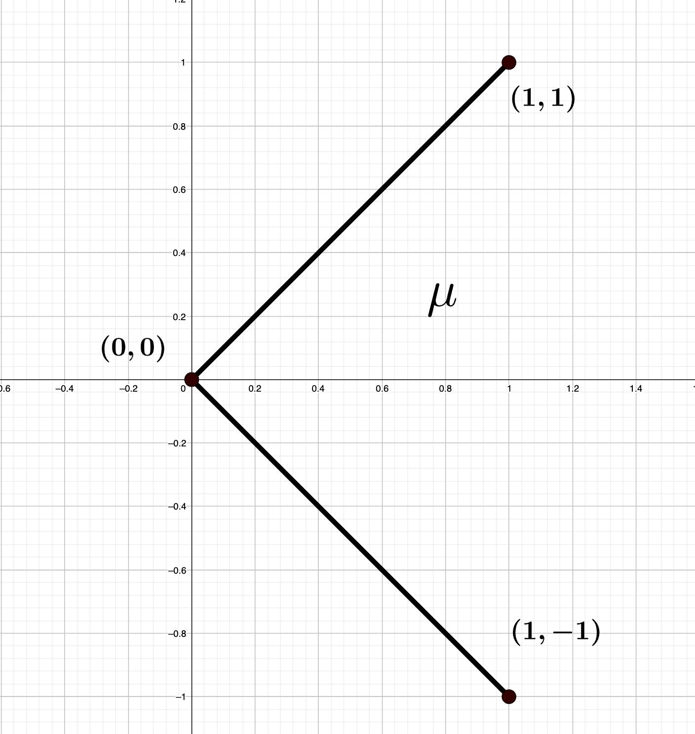
(a) $\mu=\frac{1}{2}\delta_{(0,1)}+\frac{1}{2}\delta_{(0,-1)}$

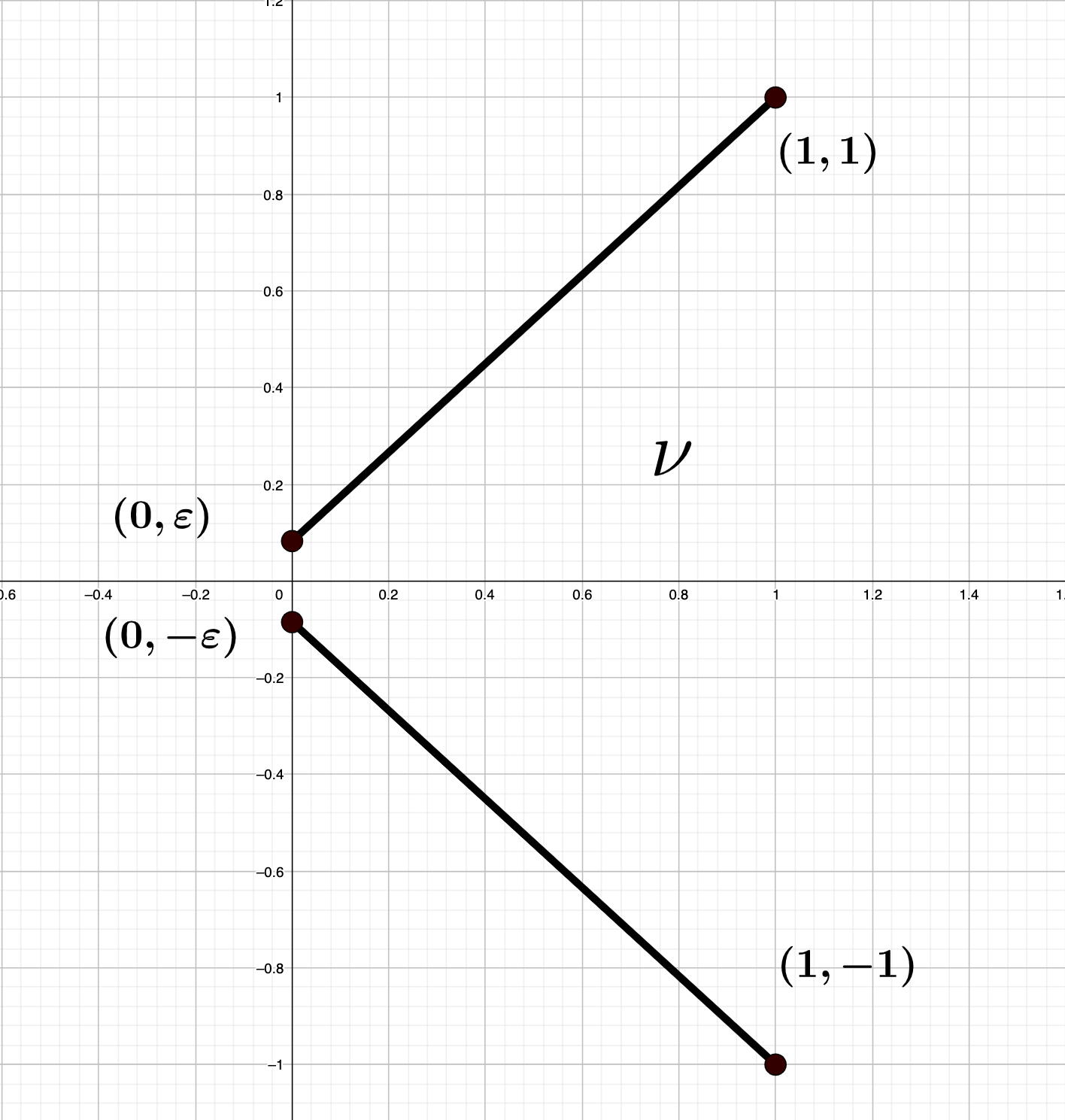
(b) $\nu=\frac{1}{2}\delta_{(\epsilon,1)}+\frac{1}{2}\delta_{(-\epsilon,-1)}$

Figure 1: Visualization of $\mu$ and $\nu$.

Let us now consider a financial market with an asset whose law is described by $\mu$, and another market with an asset whose law is described by $\nu$. Then under the Wasserstein distance the two markets are judged as being close to each other, while they clearly present very different features (random versus deterministic evolution, no-arbitrage versus arbitrage, etc.). It is also evident how optimization problems in the two situations would lead to very different decision making. This is a standard example to motivate the introduction of adapted distances, that instead can distinguish between the two models.

2.1 Adapted empirical measure

Let $\mu\in\mathcal{P}(\mathbb{R}^{dT})$, and let $(X^{(n)})_{n\in\mathbb{N}}$ be i.i.d. samples from $\mu$ defined on some probability space $(\Omega,\mathcal{F},\mathbb{P})$.

Definition 2.4 (Empirical measure).

For all $N\in\mathbb{N}$, we denote by

$$\mu^{N}=\frac{1}{N}\sum_{n=1}^{N}\delta_{X^{(n)}}$$

the empirical measure of $\mu$.

Next we introduce the adapted empirical measure on $\mathbb{R}^{dT}$ analogously to the adapted empirical measure defined on $[0,1]^{dT}$ in [Bac+22].

Definition 2.5 ((Uniform) adapted empirical measure).

For $N\in\mathbb{N}$ and grid size $\Delta_{N}>0$, we let $m=\lceil\frac{1}{\Delta_{N}}\rceil$ and consider the uniform partition $\hat{\Phi}$ of $\mathbb{R}^{dT}$ given by

$$\hat{\Phi}^{N}=\left\{\hat{\mathcal{C}}_{\mathbf{z}}^{N}=\Big{[}0,\frac{1}{m}\Big{]}^{dT}+\frac{1}{m}\mathbf{z},\mathbf{z}\in\mathbb{Z}^{dT}\right\}.$$ (3)

Let $\hat{\Lambda}^{N}$ be the set of mid points of all cubes $\hat{\mathcal{C}}_{\mathbf{z}}^{N}$ in the partition $\hat{\Phi}^{N}$, and let $\hat{\varphi}^{N}\colon\mathbb{R}^{dT}\to\hat{\Lambda}^{N}$ map each cube $\hat{\mathcal{C}}_{\mathbf{z}}^{N}$ to its mid point (points belonging to more than one cube can be mapped into any of them). Then we denote by

$$\hat{\mu}^{N}=\frac{1}{N}\sum_{n=1}^{N}\delta_{\hat{\varphi}^{N}(X^{(n)})}$$

the (uniform) adapted empirical measure of $\mu$ with grid size $\Delta_{N}$.

Intuitively, the adapted empirical measure is constructed via the following procedure: we tile $\mathbb{R}^{dT}$ with cubes of size $(\frac{1}{m})^{dT}$ that form the partition $\hat{\Phi}^{N}$, then we project all points in each cube $\hat{\mathcal{C}}_{\mathbf{z}}^{N}$ to its mid point, see Figure 2(a). As a result, the push-forward measure obtained as empirical measure of the samples after projections is indeed the adapted empirical measure.

On the other hand, if we tile $\mathbb{R}^{dT}$ with cubes of different sizes, then we obtain a non-uniform partition, on which we can similarly consider a projection and from it define a non-uniform adapted empirical measure. For the purpose of this paper, we consider the partition which is denser around the origin and coarser when far from it.

Definition 2.6 (Non-uniform adapted empirical measure).

For $N\in\mathbb{N}$ and grid size $\Delta_{N}>0$, we let $m=\lceil\frac{1}{\Delta_{N}}\rceil$, $\mathcal{A}_{0}=[-1,1]^{dT}$. Let $\mathcal{A}_{j}=[-2^{j},2^{j}]^{dT}{\color[rgb]{0,0,0}\backslash}[-2^{j-1},2^{j-1}]^{dT},j\in\mathbb{N},$ be cubic rings and

$$\check{\Phi}^{N}=\bigcup_{j=0}^{\infty}\check{\Phi}^{N,j}=\bigcup_{j=0}^{\infty}\left\{\check{\mathcal{C}}_{\mathbf{z}}^{N,j}=\Big{[}0,\frac{2^{j-1}}{m}\Big{]}^{dT}+\frac{2^{j-1}}{m}\mathbf{z}\subseteq\mathcal{A}_{j},\mathbf{z}\in\mathbb{Z}^{dT}\right\}.$$ (4)

Let $\check{\Lambda}^{N}$ be the set of mid points of all cubes $\check{\mathcal{C}}_{\mathbf{z}}^{N,j}$ in the partition $\check{\Phi}^{N}$, and let $\check{\varphi}^{N}\colon\mathbb{R}^{dT}\to\check{\Lambda}^{N}$ map each cube $\check{\mathcal{C}}_{\mathbf{z}}^{N,j}$ to its mid point. Then we denote by

$$\check{\mu}^{N}=\frac{1}{N}\sum_{n=1}^{N}\delta_{\check{\varphi}^{N}(X^{(n)})}$$

the non-uniform adapted empirical measure of $\mu$ with grid size $\Delta_{N}$.

Intuitively, we first partition $\mathbb{R}^{dT}$ into cubic rings $\mathcal{A}_{j}$, $j=0,1,2,...$, and then partition each ring $\mathcal{A}_{j}$ into subcubes of size $(\frac{2^{j-1}}{m})^{dT}$, see Figure 2(b). By doing this, we avoid considering a fine partition when we are far from the origin where less mass of the measure lies.

Throughout the paper, we will use the following notation. We use the symbol $\wedge$ for notations related to the (uniform) adapted empirical measure, such as $\hat{\mu}^{N},\hat{\Phi}^{N},\hat{\Phi}^{N}_{t},\hat{\varphi}^{N},\hat{\Lambda}^{N}$, and the symbol $\vee$ for notations related to the non-uniform adapted empirical measure, such as $\check{\mu}^{N},\check{\Phi}^{N},\check{\Phi}^{N}_{t},\check{\varphi}^{N},\check{\Lambda}^{N}$. If a statement holds for both uniform and non-uniform cases, we instead adopt the notations $\bar{\mu}^{N},\Phi^{N},\Phi^{N}_{t},\Lambda^{N}_{t},\varphi^{N}_{t}$, where we use the bar symbol on the measure to avoid duplication of the notation $\mu^{N}$, which we use for the classical empirical measure. We let $\Delta_{N}=N^{-\frac{1}{dT}}$, for all $N\in\mathbb{N}$.

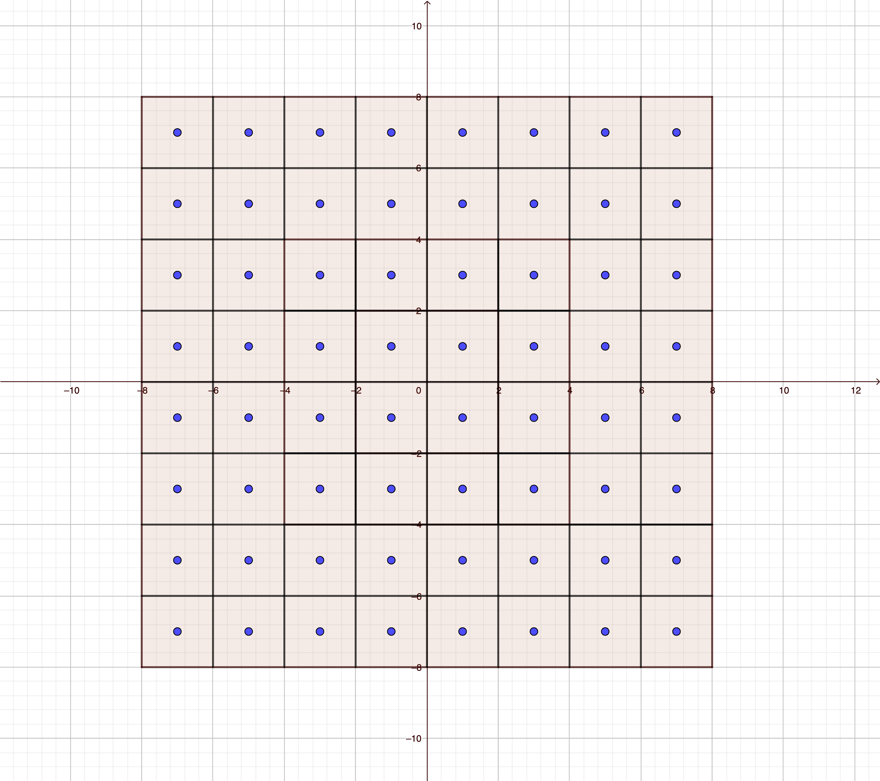
(a) Uniform grid

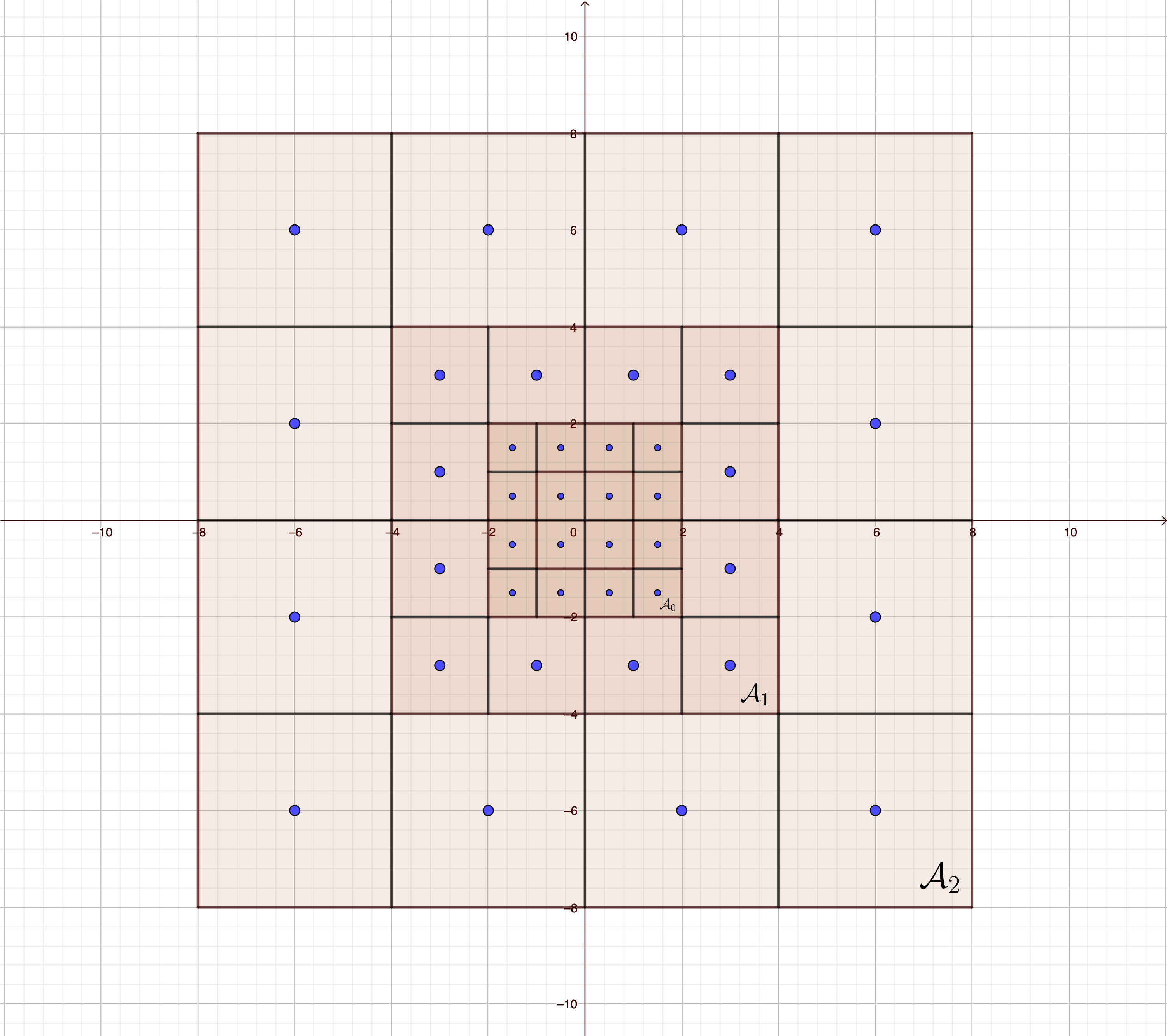
(b) Non-uniform gird

Figure 2: Visualization of uniform grid and non-uniform grid.

2.2 Main results

Our first main theorem is the following consistency result: the adapted empirical measure converges almost surely to the underlying measure $\mu$ under adapted Wasserstein distance, as long as $\mu$ is integrable; see Section 7 for the proof.

Theorem 2.7 (Almost sure convergence).

Let $\mu\in\mathcal{P}(\mathbb{R}^{dT})$ be integrable. Then

$$\lim_{N\to\infty}\mathcal{AW}(\mu,\hat{\mu}^{N})=0\quad\mathbb{P}\text{-a.s.}$$

and

$$\lim_{N\to\infty}\mathcal{AW}(\mu,\check{\mu}^{N})=0\quad\mathbb{P}\text{-a.s.}$$

It is worth noticing that integrability is the mildest assumption here because at least we need $\mathcal{AW}(\mu,\mu^{N})$ to be finite. In order to further quantify the speed of convergence for $\mu\in\mathcal{P}(\mathbb{R}^{dT})$, integrability is not enough anymore. Then we need two more regularity assumptions: the uniform moment noise condition and the uniform Lipschitz kernel condition.

For $p\geq 1$, we denote by $M_{p}(\mu)=\int\|x\|^{p}\mu(dx)$ the $p$-th moment of $\mu$, and for $\alpha,\gamma>0$, we denote by $\mathcal{E}_{\alpha,\gamma}(\mu)=\int\exp\Big{(}\gamma\|x\|^{\alpha}\Big{)}\mu(dx)$ the $(\alpha,\gamma)$-exponential moment of $\mu$. Besides the moment condition in [FG15] on the underlying measure, we would also assume some moment condition on kernels. The simplistic way to require this, would be to assume uniform moment of kernels i.e. $\sup_{x_{1:t}\in\mathbb{R}^{dt}}M_{p}(\mu_{x_{1:t}})<\infty$ for all $t=1,\dots,T-1$. However, this is such a strong condition that even the discretized Black-Scholes model (with simplest dynamic: $X_{t+1}=X_{t}+X_{t}\Delta W_{t}$) fails to satisfy! Motivated by this, we define the uniform moment noise assumption based on kernel decomposition. We start by noticing that, for every $\mu\in\mathcal{P}(\mathbb{R}^{dT})$ and for all $t=1,\dots,T-1$ and $x_{1:t}\in\mathbb{R}^{d}$, the kernel $\mu_{x_{1:t}}$ admits the following decomposition:

$$\mu_{x_{1:t}}\sim f_{t}(x_{1:t})+\sigma_{t}(x_{1:t})\cdot\varepsilon_{x_{1:t}},$$

where $f_{t}\colon\mathbb{R}^{dt}\to\mathbb{R}^{d}$, $\sigma_{t}\colon\mathbb{R}^{dt}\to\mathbb{R}_{\geq 0}$, and $\varepsilon_{x_{1:t}}$ is an $\mathbb{R}^{d}$-valued random variable depending on $x_{1:t}$. Indeed, to see this it suffices to consider the following decomposition of $(X_{t})_{t=1}^{T}\sim\mu$, for any $p\geq 1$ s.t. $M_{p}(\mu)<\infty$:

$$X_{t+1}=\mathbb{E}[X_{t+1}|\mathcal{F}^{X}_{t}]+\mathbb{E}\Big{[}\big{|}X_{t+1}-\mathbb{E}[X_{t+1}|\mathcal{F}^{X}_{t}]\big{|}^{p}\Big{|}\mathcal{F}^{X}_{t}\Big{]}^{1/p}\frac{X_{t+1}-\mathbb{E}[X_{t+1}|\mathcal{F}^{X}_{t}]}{\mathbb{E}\Big{[}\big{|}X_{t+1}-\mathbb{E}[X_{t+1}|\mathcal{F}^{X}_{t}]\big{|}^{p}\Big{|}\mathcal{F}^{X}_{t}\Big{]}^{1/p}},$$ (5)

where ${(\mathcal{F}^{X}_{t})}_{t}$ is the filtration generated by $(X_{t})_{t}$.

Definition 2.8 (Uniform moment noise kernel).

Let $\mu\in\mathcal{P}(\mathbb{R}^{dT})$, $r\geq 0$, $p\geq 1$ (resp. $\alpha,\gamma>0$). We say that $\mu$ has uniform $p$-th moment (resp. uniform $(\alpha,\gamma)$-exponential moment) noise kernel of growth $r$ if there exist $c>0$, $f_{t}\colon\mathbb{R}^{dt}\to\mathbb{R}^{d}$, $\sigma_{t}\colon\mathbb{R}^{dt}\to\mathbb{R}_{\geq 0}$ and $\lambda_{x_{1:t}}\in\mathcal{P}(\mathbb{R}^{d})$ s.t., for all $t=1,\dots,T-1$, $x_{1:t}\in\mathbb{R}^{dt}$,

$$\mu_{x_{1:t}}\sim f_{t}(x_{1:t})+\sigma_{t}(x_{1:t})\cdot\varepsilon_{x_{1:t}},\quad\varepsilon_{x_{1:t}}\sim\lambda_{x_{1:t}},$$ (6)

with $\sigma_{t}(x_{1:t})\leq c\|x_{1:t}\|^{r}$ and $\sup_{x_{1:t}\in\mathbb{R}^{dt}}M_{p}(\lambda_{x_{1:t}})<\infty$ (resp. $\sup_{x_{1:t}\in\mathbb{R}^{dt}}\mathcal{E}_{\alpha,\gamma}(\lambda_{x_{1:t}})<\infty$).

Remark 2.9.

If we consider $f_{t}=0$ and $\sigma_{t}=1$ for all $t=1,\dots,T-1$, then the uniform moment noise kernel condition boils down to the uniform moment kernel condition, i.e. $\sup_{x_{1:t}\in\mathbb{R}^{dt}}M_{p}(\mu_{x_{1:t}})<\infty$ for all $t=1,\dots,T-1$. In this case, one can directly follow the proof in [Bac+22] without involving the shifting and scaling kernels technique, but still using different estimations than those in [Bac+22], in order to deal with the infinite sum of error terms when the support is not compact.

Moreover, by the kernel decomposition (5), we can directly see from Definition 2.8 that as long as $(X_{t})_{t=1}^{T}\sim\mu$ satisfies

$$\sup_{x_{1:t}\in\mathbb{R}^{dt}}M_{p}\left(\frac{X_{t+1}-\mathbb{E}[X_{t+1}|X_{1:t}=x_{1:t}]}{\|x_{1:t}\|^{r}}\right)<\infty,$$

then $\mu$ has uniform $p$-th moment noise kernels of growth $r$. This gives a general way to test whether a distribution has uniform moment noise kernel. Next, we introduce the uniform Lipschitz kernels in the same fashion of [PP16, Bac+22].

Definition 2.10.

We say that $\mu\in\mathcal{P}(\mathbb{R}^{dT})$ has $L$-Lipschitz kernels if there exists a disintegration of $\mu$ such that, for all $t=1,\dots,T-1$,

$$\mathbb{R}^{dt}\ni(x_{1},\dots,x_{t})\mapsto\mu_{x_{1:t}}\in\mathcal{P}(\mathbb{R}^{d})$$

is $L$-Lipschitz continuous on $\mathbb{R}^{dt}$, where $\mathcal{P}(\mathbb{R}^{d})$ is endowed with Wasserstein distance.

We show below two examples where both the uniform moment noise and the uniform Lipschitz kernel conditions hold.

Example 2.11 (Discretized Black Scholes model).

Let $\mu\in\mathcal{P}(\mathbb{R}^{dT})$ be the law of the discretized Black Scholes model, satisfying $\mu_{1}=\delta_{\mathbf{1}}$ and

$$\mu_{x_{1:t}}\sim{\color[rgb]{0,0,0}x_{t}}+\sqrt{\Delta t}\,{\color[rgb]{0,0,0}x_{t}}\cdot\varepsilon_{t},$$

where $\varepsilon_{t}\sim\mathcal{N}(0,\mathbf{I}_{d})$ i.i.d. for all $t=1,\dots,T-1$. Notice that

$$\begin{split}\mathcal{W}(\mu_{x_{1:t}},\mu_{x^{\prime}_{1:t}})\leq\mathcal{W}_{2}(\mu_{x_{1:t}},\mu_{x^{\prime}_{1:t}})&\leq\sqrt{\|{\color[rgb]{0,0,0}x_{t}}-{\color[rgb]{0,0,0}x^{\prime}_{t}}\|^{2}+\|\sqrt{\Delta t}{\color[rgb]{0,0,0}x_{t}}-\sqrt{\Delta t}{\color[rgb]{0,0,0}x^{\prime}_{t}}\|^{2}\mathrm{Trace}(\mathbf{I}_{d})}\\ &\leq(1+d\Delta t)^{\frac{1}{2}}\|{\color[rgb]{0,0,0}x_{t}}-{\color[rgb]{0,0,0}x^{\prime}_{t}}\|\leq{\color[rgb]{0,0,0}(1+d\Delta t)^{\frac{1}{2}}\|x_{1:t}-x^{\prime}_{1:t}\|}.\end{split}$$

Then, for all $p,q>0$, $\mu$ has finite $q$-th moment and $(1+dt)^{\frac{1}{2}}$-Lipschitz, uniform $p$-th moment kernels of growth $1$.

Example 2.12 (Discretized SDE).

Let us consider the following SDE:

$$dX_{t}=\mu(t,X_{t})dt+\sigma(t,X_{t})dW_{t},$$

where $\mu$ and $\sigma$ are Lipschitz w.r.t. the second argument. The corresponding discretized SDE then reads as

$$X_{t+1}=X_{t}+\mu(t,X_{t})\Delta t+\sigma(t,X_{t})\sqrt{\Delta t}\epsilon_{t},$$

where $(\epsilon_{t})_{t}$ are independent standard normal random variables. Notice that, as $\mu$ and $\sigma$ are Lipschitz, they have at most linear growth. We conclude that the solution of the above discretized SDE has uniform exponential moment noise of growth $1$ and Lipschitz kernels.

Remark 2.13.

Many other benchmark models in mathematical finance satisfy uniform moment noise kernels, e.g. the GARCH model and the Heston model with clipped volatility, which could be checked similarly as in Example 2.12.

Recall that under the classical Wasserstein distance, the rates are as follows:

$$\mathbb{E}[\mathcal{W}_{1}(\mu,\mu^{N})]\leq\left\{\begin{aligned} &CN^{-\frac{1}{2}},\quad&d=1\\ &CN^{-\frac{1}{2}}\log(N),\quad&d=2\\ &CN^{-\frac{1}{d}},\quad&d\geq 3\end{aligned}\right\}\leq CN^{-\frac{1}{\mathcal{D}(d)}},$$

where $\mathcal{D}\colon\mathbb{N}\to\mathbb{N}$ is defined as

$$\mathcal{D}(d)=\left\{\begin{aligned} &d+1,&d=1,2\\ &d,&d\geq 3\end{aligned}\right..$$

Now, we are ready to state our main speed of convergence result. Since moment conditions for the same convergence rate are slightly different between the uniform and non-uniform adapted empirical measures, we consider the following two settings.

Setting 2.14.

Let $r\geq 0$, $p\geq 1$, $q>\max\left\{\frac{{\color[rgb]{0,0,0}\mathcal{D}(d)}}{{\color[rgb]{0,0,0}\mathcal{D}(d)}-1}(r+T-1),rp+{\color[rgb]{0,0,0}\mathcal{D}(d)}(T-1)(p-1)\right\}$, and let $\mu\in\mathcal{P}(\mathbb{R}^{dT})$ with finite $q$-th moment and $L$-Lipschitz, uniform $p$-th moment kernels of growth $r$. Moreover, let $L_{f}>0$ and assume that $f_{t}$ in (6) is $L_{f}$-Lipschitz for all $t=1,\dots,T-1$.

Setting 2.15.

Let $r\geq 0$, $p\geq 1$, $q>\max\left\{\frac{r{\color[rgb]{0,0,0}\mathcal{D}(d)}}{{\color[rgb]{0,0,0}\mathcal{D}(d)}-1},(r+1)p\right\}$, and let $\mu\in\mathcal{P}(\mathbb{R}^{dT})$ with finite $q$-th moment and $L$-Lipschitz, uniform $p$-th moment kernels of growth $r$. Moreover, let $L_{f}>0$ and assume that $f_{t}$ in (6) is $L_{f}$-Lipschitz for all $t=1,\dots,T-1$.

First we estimate the speed of the expected error; see Section 4 for the proof.

Theorem 2.16 (Moment estimate).

Let $p,q>1$.

1. Under Setting 2.14, there exists a constant $C>0$ s.t., for all $N\in\mathbb{N}$,

   $$\mathbb{E}\big{[}\mathcal{AW}(\mu,\hat{\mu}^{N})\big{]}\leq CN^{-\frac{1}{{\color[rgb]{0,0,0}\mathcal{D}(d)}T}}+CN^{-\frac{p-1}{pT}}.$$

2. Under Setting 2.15, there exists a constant $C>0$ s.t., for all $N\in\mathbb{N}$,

   $$\mathbb{E}\big{[}\mathcal{AW}(\mu,\check{\mu}^{N})\big{]}\leq CN^{-\frac{1}{{\color[rgb]{0,0,0}\mathcal{D}(d)}T}}+CN^{-\frac{p-1}{pT}}.$$

When $p>1+\frac{1}{{\color[rgb]{0,0,0}\mathcal{D}(d)}-1}$, $N^{-\frac{1}{{\color[rgb]{0,0,0}\mathcal{D}(d)}T}}$ dominates the right hand side in the two above estimates. Next, we estimate the speed of deviation error; see Section 5 for the proof.

Theorem 2.17 (Concentration inequality I).

Let $p,q>2$ and $\mathrm{rate}(N)=\mathcal{O}(N^{-\frac{1}{{\color[rgb]{0,0,0}\mathcal{D}(d)}T}})$.

1. Assume Setting 2.14. Then, for all $\epsilon\in(0,p-2)$, there exists a constant $C>0$ s.t., for all $N\in\mathbb{N}$ and $x>0$,

   $$\mathbb{P}\Big{[}\mathcal{AW}(\mu,\hat{\mu}^{N})\geq x+\mathrm{rate}(N)\Big{]}\leq{\color[rgb]{0,0,0}CN^{-\frac{p-\epsilon}{{\color[rgb]{0,0,0}\mathcal{D}(d)}T}}x^{-p+\epsilon}}.$$

2. Assume Setting 2.15. Then, for all $\epsilon\in(0,p-2)$, there exists a constant $C>0$ s.t., for all $N\in\mathbb{N}$ and $x>0$,

   $$\mathbb{P}\Big{[}\mathcal{AW}(\mu,\check{\mu}^{N})\geq x+\mathrm{rate}(N)\Big{]}\leq{\color[rgb]{0,0,0}CN^{-\frac{p-\epsilon}{{\color[rgb]{0,0,0}\mathcal{D}(d)}T}}x^{-p+\epsilon}}+CN^{-\frac{p}{2}}x^{-p}.$$

Moreover, if we strengthen the moment condition to the exponential moment condition, we obtain the (optimal) exponential concentration inequality; see Section 6 for the proof.

Setting 2.18.

Let $\alpha\geq 2$, $\gamma>0$, $r\geq 0$, and $\mu\in\mathcal{P}(\mathbb{R}^{dT})$ with finite $(\alpha,\gamma)$-exponential moment and $L$-Lipschitz, uniform $(\alpha,\gamma)$-exponential moment kernels of growth $r$.

Theorem 2.19 (Concentration inequality II).

Assume Setting 2.18 and let $\mathrm{rate}(N)=\mathcal{O}(N^{-\frac{1}{{\color[rgb]{0,0,0}\mathcal{D}(d)}T}})$.

1. For uniform adapted empirical measures and $r=0$, there exist constants $c,C>0$ such that, for all $x\geq 0$ and $N\in\mathbb{N}$,

   $$\mathbb{P}\Big{[}\mathcal{AW}(\mu,\hat{\mu}^{N})\geq x+\mathrm{rate}(N)\Big{]}\leq Ce^{-cNx^{2}}.$$

2. For uniform adapted empirical measures and $r>0$, there exist constants $c,C>0$ such that, for all $x\geq 0$ and $N\in\mathbb{N}$ satisfying $\sqrt{N}x\geq 1$,

   $$\mathbb{P}\Big{[}\mathcal{AW}(\mu,\hat{\mu}^{N})\geq x+\mathrm{rate}(N)\Big{]}\leq CNe^{-c(\sqrt{N}x)^{\frac{1}{r+1}}}.$$

3. For non-uniform adapted empirical measures, there exist constants $c,C>0$ such that, for all $x\geq 0$ and $N\in\mathbb{N}$ satisfying $\sqrt{N}x\geq 1$,

   $$\mathbb{P}\Big{[}\mathcal{AW}(\mu,\check{\mu}^{N})\geq x+\mathrm{rate}(N)\Big{]}\leq CNe^{-c(\sqrt{N}x)^{\frac{1}{r+2}}}.$$

Theorem 2.19 (i) recovers the same optimal exponential concentration rate of compactly supported adapted empirical measures under adapted Wasserstein distance, that is Theorem 1.7 in [Bac+22]. Moreover, this is also the same exponential concentration rate of empirical measures under Wasserstein distance under exponential moment assumption, that is Theorem 2 in [FG15].

For the convenience of the reader, we recall the convergence rates of adapted empirical measures given in [Bac+22].

Theorem 2.20 (Theorem 1.3 in [Bac+22]).

Let $\mu\in\mathcal{P}([0,1]^{dT})$. Then $\lim_{N\to\infty}\mathcal{AW}(\mu,\hat{\mu}^{N})=0\quad\mathbb{P}\text{-a.s.}$.

Theorem 2.21 (Theorem 1.5 and Theorem 1.7 in [Bac+22]).

Assume $\mu\in\mathcal{P}([0,1]^{dT})$ with $L$-Lipschitz kernels. Then there exists $C>0$ s.t., for all $N\in\mathbb{N}$ and $x>0$,

$$\mathbb{E}[\mathcal{AW}(\mu,\hat{\mu}^{N})]\leq CN^{-\frac{1}{\mathcal{D}(d)T}}$$

and

$$\mathbb{P}\Big{[}\mathcal{AW}(\mu,\hat{\mu}^{N})\geq\mathrm{rate}(N)+x\Big{]}\leq Ce^{-cNx^{2}},$$

where $\mathrm{rate}(N)=\mathcal{O}(\Delta_{N})$.

Remark 2.22.

If $\mu\in\mathcal{P}([0,1]^{dT})$, then the integrability assumptions in Theorem 2.7, Theorem 2.16 and Theorem 2.19 hold for all $p>1$. Therefore, our results generalize those in [Bac+22]. In particular we recover the sharp rates when $d=1$ and $d\geq 3$.

When $d=2$, the sharp moment rate is of growth $N^{-\frac{1}{d}}\log(N)$. However, the $\log(N)$ term is estimated by $N^{\frac{1}{d}-\frac{1}{d+\zeta}}$ for all $\zeta>0$ in our results, in particular $\zeta=1$ in the statements of main theorems. Thus, we achieve at most a $N^{\frac{1}{d+\zeta}}$ rate for all $\zeta>0$, and not the optimal one $N^{-\frac{1}{d}}\log(N)$.

3 Notations and preparatory lemmas

We start this section by recalling some notations introduced above, and introducing some more, that will be used throughout the paper. For $t=1,\dots,T$, we denote by $\|\cdot\|_{1:t}\colon\mathbb{R}^{dt}\to\mathbb{R}$ the sum-norm on $\mathbb{R}^{dt}$ defined by $\|x_{1:t}\|_{1:t}=\sum_{s=1}^{t}\|x_{s}\|_{\mathbb{R}^{d}}$ for all $x_{1:t}=(x_{1},\dots,x_{t})\in\mathbb{R}^{dt}$. For simplicity, we unify notations of norm and write $\|x_{1:t}\|=\|x_{1:t}\|_{1:t}$ for all $x_{1:t}\in\mathbb{R}^{dt}$ and $t=1,\dots,T$. For $\mu\in\mathcal{P}(\mathbb{R}^{dT})$ and $t=1,\dots,T$, we denote by $\mu_{t}\in\mathcal{P}(\mathbb{R}^{d})$ the $t$-th marginal of $\mu$, and by $\mu_{1:t}\in\mathcal{P}(\mathbb{R}^{dt})$ the up to $t$ marginal of $\mu$, in particular $\mu_{1}$ is the first marginal. For all $\mu\in\mathcal{P}(\mathbb{R}^{dT})$ and Borel sets $G\subseteq\mathbb{R}^{dt}$, $t=1,\dots,T$, we also unify notations of marginals and denote $\mu(G)=\mu_{1:t}(G)$. For all $x_{1:t}\in\mathbb{R}^{dt}$, $t=1,\dots,T-1$, we denote by $\mu_{x_{1:t}}\in\mathcal{P}(\mathbb{R}^{d})$ the kernel of $\mu$. Moreover, for all Borel sets $G\subseteq\mathbb{R}^{dt}$, $t=1,\dots,T-1$, we define the conditional law of $\mu$ on $G$ by $\mu|_{G}\in\mathcal{P}(\mathbb{R}^{dt})$:

$$\mu|_{G}({\color[rgb]{0,0,0}dx_{1:t}})=\frac{\mu(G\cap dx_{1:t})}{\mu(G)},$$

and define the average kernel of $\mu$ on $G$ by $\mu_{G}\in\mathcal{P}(\mathbb{R}^{d})$:

$$\mu_{G}(dx_{t+1})=\frac{1}{\mu(G)}\int_{G}\mu_{x_{1:t}}(dx_{t+1})\mu(dx_{1:t}).$$

If $\mu(G)=0$, w.l.o.g. we set $\mu|_{G}=\mu_{G}=\delta_{0}$ for the completeness of definition. For $G\subseteq\mathbb{R}^{dT}$, we define $\mathrm{diam}(G)=\sup_{x,y\in G}\|x-y\|$ and refer to it as the diameter of $G$, and let $\|G\|=\sup_{x\in G}\|x\|$. For example, for any cube $G=[0,\ell]^{dt}$, $\ell>0$, we have $\mathrm{diam}(G)=\|G\|=t\sqrt{d}\ell^{d}$. For $f\in\mathbb{R}^{d}$, $\sigma>0$ and $\gamma\in\mathcal{P}(\mathbb{R}^{d})$, we use the notation $\gamma+f=(x\mapsto x+f)_{\#}\gamma$ and $\sigma\gamma=(x\mapsto\sigma x)_{\#}\gamma$. Recall the notations introduced in Definitions 2.5 and 2.6 on $\mathbb{R}^{dT}$, which we can analogously define on $\mathbb{R}^{dt}$ by replacing the time dimension $T$ with $t$, e.g. $\hat{\Phi}^{N}_{t}=\big{\{}\big{[}0,\frac{1}{m}\big{]}^{dt}+\frac{1}{m}\mathbf{z},\mathbf{z}\in\mathbb{Z}^{dt}\big{\}}$ and $\mathcal{A}_{j}^{t}=[-2^{j},2^{j}]^{dt}\backslash[-2^{j-1},2^{j-1}]^{dt}$. Similarly, replacing $T$ with $t$, we define $\check{\Phi}^{N}_{t}$, $\Phi^{N}_{t}$, $\hat{\Phi}^{N,j}_{t}$, $\check{\Phi}^{N,j}_{t}$, $\Phi^{N,j}_{t}$, $\hat{\Lambda}^{N}_{t}$, $\check{\Lambda}^{N}_{t}$, $\Lambda^{N}_{t}$, $\hat{\varphi}^{N}_{t}$, $\check{\varphi}^{N}_{t}$, $\varphi^{N}_{t}$.
Convention: In our proofs, we let $C,c>0$ be generic constants that may increase from line to line depending on all sorts of external parameters, e.g. $\epsilon$ and $L$, but independent of internal parameters, e.g. $N\in\mathbb{N}$ and $x>0$. Moreover, to simplify notations, we present the proof for the case $d\geq 3$ (so that $\mathcal{D}(d)=d$), while for the general case one would need to replace $d$ by $\mathcal{D}(d)$ in the proof.

3.1 Preparatory lemmas

The uniform and non-uniform adapted partitions are different in the diameter of the cubes that form the partition, i.e. $\mathrm{diam}(G)$ for $G\in\Phi_{t}^{N}$. Thus, they are also different in the number of cubes in the same cubic ring, which we denote by $|\Phi^{N,j}_{t}|$. In fact, we have the following estimates of $\mathrm{diam}(G)$ and $|\Phi^{N,j}_{t}|$:

• For all $t=1,\dots,T$, $j\geq 0$, $\hat{G}\in\hat{\Phi}^{N,j}_{t}$,

  $$\mathrm{diam}(\hat{G})\leq t\sqrt{d}\Delta_{N},\quad|\hat{\Phi}^{N,j}_{t}|\leq(2^{j+1}N^{\frac{1}{dT}})^{dt}.$$ (7)

• For all $t=1,\dots,T$, $j\geq 0$, $\check{G}\in\check{\Phi}^{N,j}_{t}$,

  $$\mathrm{diam}(\check{G})\leq t\sqrt{d}2^{j}\Delta_{N},\quad|\check{\Phi}^{N,j}_{t}|\leq(4N^{\frac{1}{dT}})^{dt}.$$ (8)

Moreover, since $\Phi^{N,j}_{t}$ is a partition of $\mathcal{A}^{j}_{t}$, we also need to estimate $\mu(\mathcal{A}^{j}_{t})$ in later proofs, which is a direct consequence of Markov’s inequality:

$$\mu(\mathcal{A}^{t}_{0})\leq 1,\quad\mu(\mathcal{A}^{t}_{j})\leq\frac{M_{q}(\mu_{1:t})}{2^{q(j-1)}},~{}j\in\mathbb{N}.$$

Therefore, if we assume Setting 2.14 or Setting 2.15, then there exists $C>0$ such that

$$\mu(\mathcal{A}^{t}_{j})\leq\frac{C}{2^{q(j-1)}},~{}j\geq 0.$$ (9)

Next, we present a lemma decomposing the adapted Wasserstein distance between (uniform or non-uniform) adapted empirical measure and the underlying measure, under uniform Lipschitz kernel assumption. In this lemma, the bound for the uniform adapted empirical measure is sharper than for the non-uniform one.

Lemma 3.1.

Assume $\mu\in\mathcal{P}(\mathbb{R}^{dT})$ has $L$-Lipschitz kernels. Then

1. there exists $C>0$ s.t., for all $N\in\mathbb{N}$,

   $$\mathcal{AW}(\mu,\hat{\mu}^{N})\leq C\Big{(}\Delta_{N}+\mathcal{W}(\mu_{1},\mu^{N}_{1})+\sum_{t=1}^{T-1}\sum_{G\in\hat{\Phi}_{t}^{N}}\mu^{N}(G)\mathcal{W}(\mu_{G},\mu_{G}^{N})\Big{)};$$ (10)

2. there exists $C>0$ s.t., for all $N\in\mathbb{N}$,

   $$\mathcal{AW}(\mu,\check{\mu}^{N})\leq C\Big{(}\Delta_{N}+\mathcal{W}(\mu_{1},\mu^{N}_{1})+\sum_{t=1}^{T-1}\sum_{G\in\check{\Phi}_{t}^{N}}\mu^{N}(G)\mathcal{W}(\mu_{G},\mu_{G}^{N})\Big{)}+\frac{C\Delta_{N}}{N}\sum_{n=1}^{N}\|X^{(n)}\|.$$ (11)

Proof.

Step 1: In this step, all statements hold for both uniform and non-uniform adapted empirical measures. Recall that we use the notation $\bar{\mu}^{N}$ to denote the uniform or non-uniform adapted empirical measure. In [Bac+22], Lemma 3.1 proves that, when $\mu\in\mathcal{P}([0,1]^{dT})$,

$$\mathcal{AW}(\mu,\bar{\mu}^{N}) \leq C\mathcal{W}(\mu_{1},\bar{\mu}^{N}_{1})+C\sum_{t=1}^{T-1}\sum_{G\in\Phi_{t}^{N}}\int_{G}\mathcal{W}(\mu_{x_{1:t}},\bar{\mu}^{N}_{x_{1:t}})\bar{\mu}^{N}(dx_{1:t}).$$ (12)

Since the proof does not depend on the compactness, and therefore could be generalized to the case when $\mu\in\mathcal{P}(\mathbb{R}^{dT})$. Now, by the triangle inequality we have

$$\mathcal{W}(\mu_{1},\bar{\mu}^{N}_{1})\leq\mathcal{W}(\mu_{1},\mu^{N}_{1})+\mathcal{W}(\mu^{N}_{1},\bar{\mu}^{N}_{1}).$$ (13)

Also, noticing that $\mu^{N}_{1}(G)=\bar{\mu}^{N}_{1}(G)$ for all $G\in\Phi_{1}^{N}$, we have that

$$\mathcal{W}(\mu^{N}_{1},\bar{\mu}^{N}_{1}) \leq\sum_{G\in\Phi_{1}^{N}}\mu^{N}(G)\mathcal{W}\big{(}\mu^{N}_{1}|_{G},\bar{\mu}^{N}_{1}|_{G}\big{)}\leq\sum_{G\in\Phi_{1}^{N}}\mu^{N}(G)\mathrm{diam}(G).$$ (14)

By combining (13) and (14), we obtain

$$\mathcal{W}(\mu_{1},\bar{\mu}^{N}_{1})\leq\mathcal{W}(\mu_{1},\mu^{N}_{1})+\sum_{G\in\Phi_{1}^{N}}\mu^{N}(G)\mathrm{diam}(G).$$ (15)

Next, we estimate the second term in (12) by using the Lipschitz kernel assumption: for any $G\in\Phi_{1}^{N}$,

$$\begin{split}\int_{G}\mathcal{W}(\mu_{x_{1}},(\bar{\mu}^{N})_{x_{1}})\bar{\mu}^{N}(dg)&\leq\int_{G}\Big{(}\mathcal{W}(\mu_{x_{1}},\mu_{G})+\mathcal{W}(\mu_{G},\mu_{G}^{N})+\mathcal{W}(\mu_{G}^{N},(\bar{\mu}^{N})_{x_{1}})\Big{)}\bar{\mu}^{N}(dg)\\ &\leq\int_{G}\Big{(}L\cdot\mathrm{diam}(G)+\mathcal{W}(\mu_{G},\mu_{G}^{N})+\mathcal{W}(\mu_{G}^{N},\bar{\mu}_{G}^{N})\Big{)}\bar{\mu}^{N}(dg)\\ &\leq\mu^{N}(G)\Big{(}L\cdot\mathrm{diam}(G)+\mathcal{W}(\mu_{G},\mu_{G}^{N})+\mathcal{W}(\mu_{G}^{N},\bar{\mu}_{G}^{N})\Big{)}.\end{split}$$ (16)

Combining (12), (15) and (16), we conclude for both uniform and non-uniform adapted empirical measures that there exists $C>0$ such that

$$\mathcal{AW}(\mu,\bar{\mu}^{N})\leq C\mathcal{W}(\mu_{1},\mu^{N}_{1})+C\sum_{t=1}^{T-1}\sum_{G\in\Phi_{t}^{N}}\mu^{N}(G)\Big{(}\mathcal{W}(\mu_{G},\mu_{G}^{N})+\mathcal{W}(\mu_{G}^{N},\bar{\mu}_{G}^{N})\Big{)}+C\sum_{t=1}^{T-1}\sum_{G\in\Phi_{t}^{N}}\mu^{N}(G)\mathrm{diam}(G).$$ (17)

Step 2: In this step, we separate the proof between uniform and non-uniform adapted empirical measures.
(i) Recall that we denote by $\hat{\mu}^{N}$ the uniform adapted empirical measure, then by (7) we have for all $t=1,\dots,T$ that

$$\sum_{G\in\hat{\Phi}_{t}^{N}}\mu^{N}(G)\mathrm{diam}(G)\leq t\sqrt{d}\Delta_{N}\quad\text{and}\quad\sum_{G\in\hat{\Phi}_{t}^{N}}\mu^{N}(G)\mathcal{W}(\mu_{G}^{N},\hat{\mu}_{G}^{N})\leq\sqrt{d}\Delta_{N}.$$ (18)

Combining (17) and (18), we conclude that there exists $C>0$ such that

$$\begin{split}\mathcal{AW}(\mu,\hat{\mu}^{N})&\leq C\Big{(}\Delta_{N}+\mathcal{W}(\mu_{1},\mu^{N}_{1})+\sum_{t=1}^{T-1}\sum_{G\in\hat{\Phi}_{t}^{N}}\mu^{N}(G)\mathcal{W}(\mu_{G},\mu_{G}^{N})\Big{)}.\end{split}$$ (19)

(ii) Recall that we denote by $\check{\mu}^{N}$ the non-uniform adapted empirical measure, then by (8) we have for all $t=1,\dots,T$ that

$$\begin{split}\sum_{G\in\check{\Phi}_{t}^{N}}\mu^{N}(G)\mathrm{diam}(G)&=\sum_{j=0}^{\infty}\sum_{G\in\check{\Phi}_{t}^{N,j}}\mathrm{diam}(G)\mu^{N}(G)\leq\sum_{j=0}^{\infty}\sum_{G\in\check{\Phi}_{t}^{N,j}}t\sqrt{d}\Delta_{N}2^{j}\mu^{N}(G)=t\sqrt{d}\Delta_{N}\sum_{j=0}^{\infty}2^{j}\mu^{N}(\mathcal{A}_{j}^{t}),\end{split}$$ (20)

and

$$\begin{split}\sum_{G\in\check{\Phi}_{t}^{N}}\mu^{N}(G)\mathcal{W}(\mu_{G}^{N},\check{\mu}_{G}^{N})&\leq\sum_{G\in\check{\Phi}_{t}^{N}}\mu^{N}(G)\sum_{j=0}^{\infty}\sum_{G^{\prime}\in\check{\Phi}_{1}^{N,j}}\mathrm{diam}(G^{\prime})\mu^{N}_{G}(G^{\prime})\leq\sum_{G\in\check{\Phi}_{t}^{N}}\mu^{N}(G)\sum_{j=0}^{\infty}\sum_{G^{\prime}\in\check{\Phi}_{1}^{N,j}}t\sqrt{d}\Delta_{N}2^{j}\mu^{N}_{G}(G^{\prime})\\ &=t\sqrt{d}\Delta_{N}\sum_{j=0}^{\infty}\sum_{G\in\check{\Phi}_{t}^{N}}\mu^{N}(G)\mu^{N}_{G}(\mathcal{A}_{j}^{1})2^{j}\leq t\sqrt{d}\Delta_{N}\sum_{j=0}^{\infty}2^{j}\mu_{t+1}^{N}(\mathcal{A}_{j}^{1}).\end{split}$$ (21)

Noticing that $\min_{x\in\mathcal{A}_{j}^{t}}\|x\|\geq 2^{j-1}$ for all $j\in\mathbb{N}$ and $t=1,\dots,T-1$, we have

$$\begin{split}t\sqrt{d}\Delta_{N}\sum_{j=0}^{\infty}2^{j}\mu^{N}(\mathcal{A}_{j}^{t})&\leq t\sqrt{d}\Delta_{N}+2t\sqrt{d}\Delta_{N}\sum_{j=1}^{\infty}2^{j-1}\mu^{N}(\mathcal{A}_{j}^{t})\leq t\sqrt{d}\Delta_{N}+2t\sqrt{d}\Delta_{N}\int_{\mathbb{R}^{dT}}\|x_{1:t}\|\mu^{N}(dx)\\ &\leq T\sqrt{d}\Delta_{N}+2T\sqrt{d}\Delta_{N}\int_{\mathbb{R}^{dT}}\|x\|\mu^{N}(dx)=T\sqrt{d}\Delta_{N}+\frac{2T\sqrt{d}\Delta_{N}}{N}\sum_{n=1}^{N}\|X^{(n)}\|,\\ t\sqrt{d}\Delta_{N}\sum_{j=0}^{\infty}2^{j}\mu^{N}_{t+1}(\mathcal{A}_{j}^{1})&\leq t\sqrt{d}\Delta_{N}+2t\sqrt{d}\Delta_{N}\sum_{j=1}^{\infty}2^{j-1}\mu^{N}_{t+1}(\mathcal{A}_{j}^{1})\leq t\sqrt{d}\Delta_{N}+2t\sqrt{d}\Delta_{N}\int_{\mathbb{R}^{dT}}\|x_{t+1}\|\mu^{N}(dx)\\ &\leq T\sqrt{d}\Delta_{N}+2T\sqrt{d}\Delta_{N}\int_{\mathbb{R}^{dT}}\|x\|\mu^{N}(dx)=T\sqrt{d}\Delta_{N}+\frac{2T\sqrt{d}\Delta_{N}}{N}\sum_{n=1}^{N}\|X^{(n)}\|.\end{split}$$ (22)

Combining (17), (20), (21) and (22), we conclude that there exists $C>0$ such that, for all $N\in\mathbb{N}$,

$$\mathcal{AW}(\mu,\check{\mu}^{N})\leq C\Big{(}\Delta_{N}+\mathcal{W}(\mu_{1},\mu^{N}_{1})+\sum_{t=1}^{T-1}\sum_{G\in\check{\Phi}_{t}^{N}}\mu^{N}(G)\mathcal{W}(\mu_{G},\mu_{G}^{N})\Big{)}+\frac{C\Delta_{N}}{N}\sum_{n=1}^{N}\|X^{(n)}\|.$$ (23)

Therefore, (19) and (23) together complete the proof of Lemma 3.1. ∎

In the next Lemma, we show that, conditioning on the adapted empirical law up to time $t$, the average kernel of the empirical law is the same as the empirical law of the average kernel.

Lemma 3.2.

Let $E$ be a Borel set in $\mathcal{P}(\mathbb{R}^{d})$. Then, for all $G\in\Phi_{t}^{N}$,

$$\mathbb{P}\Big{[}\mu_{G}^{N}\in E\Big{|}\mu^{N}(G^{\prime}),\forall G^{\prime}\in\Phi_{t}^{N}\Big{]}=\mathbb{P}\Big{[}\mu_{G}^{N}\in E\Big{|}\mu^{N}(G)\Big{]}=\mathbb{P}\big{[}(\mu_{G})^{N\mu^{N}(G)}\in E\Big{]},$$ (24)

where $(\mu_{G})^{N\mu^{N}(G)}$ is the empirical measure of $\mu_{G}$ with sample size $N\mu^{N}(G)\in\mathbb{N}$. Moreover, $(\mu_{G}^{N})_{G\in\Phi^{N}_{t}}$ are independent given $\{\mu^{N}(G^{\prime})\colon G^{\prime}\in\Phi_{t}^{N}\}$.

Proof.

(24) follows from the proof of Lemma 3.3 in [Bac+22], where $\mu\in\mathcal{P}([0,1]^{dT})$. Indeed, that proof does not depend on the compactness of the support of $\mu$, and can be generalized to any $\mu\in\mathcal{P}(\mathbb{R}^{dT})$. ∎

We conclude this preparatory section by estimating moments and exponential moments of shifted and scaled $\mu_{G}$.

Lemma 3.3.

Let $\mu\in\mathcal{P}(\mathbb{R}^{dT})$.

1. Assume Setting 2.14 or Setting 2.15. Then, for all $t=1,\dots,T-1$, $G\in\Phi^{N}_{t}$, there exist $f_{G}\in\mathbb{R}^{d}$ and $\sigma_{G},\lambda_{G}>0$ s.t.

   $$M_{p}^{1/p}\Big{(}\frac{1}{\lambda_{G}}\frac{\mu_{G}-f_{G}}{\sigma_{G}}\Big{)}\leq 1,$$ (25)

   where $\sigma_{G}=\sup_{x_{1:t}\in G}\sigma_{t}(x_{1:t})\vee 1$ and $\lambda_{G}=L_{f}\cdot\mathrm{diam}(G)+\big{(}\sup_{x_{1:t}\in\mathbb{R}^{dt}}M_{p}(\lambda_{x_{1:t}})\big{)}^{1/p}$.

2. Assume Setting 2.18. Then, for all $t=1,\dots,T-1$, $G\in\Phi^{N}_{t}$, there exist $f_{G}\in\mathbb{R}^{d}$ and $\sigma_{G},\lambda_{G}>0$ s.t.

   $$\mathcal{E}_{1,\alpha}\Big{(}\frac{1}{\lambda_{G}}\frac{\mu_{G}-f_{G}}{\sigma_{G}}\Big{)}\leq e\cdot\Big{(}\sup_{x_{1:t}\in\mathbb{R}^{dt}}\mathcal{E}_{\gamma,\alpha}(\lambda_{x_{1:t}})\Big{)},$$ (26)

   where $\sigma_{G}=\sup_{x_{1:t}\in G}\sigma_{t}(x_{1:t})\vee 1$ and $\lambda_{G}=2(L_{f}\mathrm{diam}(G)+1)+2\gamma^{-\alpha}$.

Proof.

Recall that for all $t=1,\dots,T-1$, $G\in\Phi^{N}_{t}$, $f_{G}\in\mathbb{R}^{d}$, $\sigma_{G}>0$,

$$\frac{\mu_{G}-f_{G}}{\sigma_{G}}=\int_{\mathbb{R}^{dt}}\frac{\mu_{x_{1:t}}-f_{G}}{\sigma_{G}}\mu|_{G}(dx_{1:t})=\int_{\mathbb{R}^{dt}}\frac{f_{t}(x_{1:t})-f_{G}+\sigma_{t}(x_{1:t})\lambda_{x_{1:t}}}{\sigma_{G}}\mu|_{G}(dx_{1:t}).$$

(i) First, we estimate the $p$-th moment under Setting 2.14 or Setting 2.15. In this case,

$$\begin{split}M_{p}^{1/p}\left(\frac{\mu_{G}-f_{G}}{\sigma_{G}}\right)&=\left(\int_{\mathbb{R}^{d}}\|x_{t+1}\|^{p}\left(\int_{\mathbb{R}^{dt}}\frac{f_{t}(x_{1:t})-f_{G}+\sigma_{t}(x_{1:t})\lambda_{x_{1:t}}}{\sigma_{G}}\mu|_{G}(dx_{1:t})\right)(dx_{t+1})\right)^{1/p}\\ &=\left(\int_{\mathbb{R}^{dt}}\int_{\mathbb{R}^{d}}\|x_{t+1}\|^{p}\frac{f_{t}(x_{1:t})-f_{G}+\sigma_{t}(x_{1:t})\lambda_{x_{1:t}}}{\sigma_{G}}(dx_{t+1})\mu|_{G}(dx_{1:t})\right)^{1/p}\\ &=\left(\int_{\mathbb{R}^{dt}}\mathbb{E}\left[\left\|\frac{f_{t}(x_{1:t})-f_{G}+\sigma_{t}(x_{1:t})\epsilon_{x_{1:t}}}{\sigma_{G}}\right\|^{p}\right]\mu|_{G}(dx_{1:t})\right)^{1/p}\\ &\leq\left(\int_{\mathbb{R}^{dt}}\left\|\frac{f_{t}(x_{1:t})-f_{G}}{\sigma_{G}}\right\|^{p}\mu|_{G}(dx_{1:t})\right)^{1/p}+\left(\int_{\mathbb{R}^{dt}}\mathbb{E}\left[\left\|\frac{\sigma_{t}(x_{1:t})\epsilon_{x_{1:t}}}{\sigma_{G}}\right\|^{p}\right]\mu|_{G}(dx_{1:t})\right)^{1/p}.\end{split}$$

By choosing $x_{G}$ as the mid point of the cube $G$, $f_{G}=f_{t}(x_{G})$ and $\sigma_{G}=\sup_{x_{1:t}\in G}\sigma_{t}(x_{1:t})\vee 1$, we have

$$\begin{split}M_{p}^{1/p}\left(\frac{\mu_{G}-f_{G}}{\sigma_{G}}\right)&\leq\left(\int_{\mathbb{R}^{dt}}\left\|f_{t}(x_{1:t})-f_{G}\right\|^{p}\mu|_{G}(dx_{1:t})\right)^{1/p}+\left(\int_{\mathbb{R}^{dt}}\mathbb{E}\left[\left\|\epsilon_{x_{1:t}}\right\|^{p}\right]\mu|_{G}(dx_{1:t})\right)^{1/p}\\ &\leq L_{f}\cdot\mathrm{diam}(G)+\Big{(}\sup_{x_{1:t}\in\mathbb{R}^{dt}}M_{p}(\lambda_{x_{1:t}})\Big{)}^{1/p}<\infty.\end{split}$$

Therefore, by choosing $\lambda_{G}=L_{f}\cdot\mathrm{diam}(G)+\Big{(}\sup_{x_{1:t}\in\mathbb{R}^{dt}}M_{p}(\lambda_{x_{1:t}})\Big{)}^{1/p}$, we get (25).
(ii) Next, we estimate the exponential moment under Setting 2.18. For any $\tilde{\gamma}>0$,

$$\begin{split}\mathcal{E}_{\tilde{\gamma},\alpha}\left(\frac{\mu_{G}-f_{G}}{\sigma_{G}}\right)&=\int_{\mathbb{R}^{dt}}\int_{\mathbb{R}^{d}}e^{\tilde{\gamma}\|x_{t+1}\|^{\alpha}}\frac{f_{t}(x_{1:t})-f_{G}+\sigma_{t}(x_{1:t})\lambda_{x_{1:t}}}{\sigma_{G}}(dx_{t+1})\mu|_{G}(dx_{1:t})\\ &=\int_{\mathbb{R}^{dt}}\mathbb{E}\left[\exp\left\{\tilde{\gamma}\left\|\frac{f_{t}(x_{1:t})-f_{G}+\sigma_{t}(x_{1:t})\epsilon_{x_{1:t}}}{\sigma_{G}}\right\|^{\alpha}\right\}\right]\mu|_{G}(dx_{1:t})\\ &\leq\int_{\mathbb{R}^{dt}}\exp\left\{2^{\alpha}\tilde{\gamma}\left\|\frac{f_{t}(x_{1:t})-f_{G}}{\sigma_{G}}\right\|^{\alpha}\right\}\mathbb{E}\left[\exp\left\{2^{\alpha}\tilde{\gamma}\left\|\frac{\sigma_{t}(x_{1:t})\epsilon_{x_{1:t}}}{\sigma_{G}}\right\|^{\alpha}\right\}\right]\mu|_{G}(dx_{1:t}).\end{split}$$

By choosing $x_{G}$ as the mid point of $G$, $f_{G}=f_{t}(x_{G})$ and $\sigma_{G}=\sup_{x_{1:t}\in G}\sigma_{t}(x_{1:t})\vee 1$ as above, we have

$$\begin{split}\mathcal{E}_{\tilde{\gamma},\alpha}\left(\frac{\mu_{G}-f_{G}}{\sigma_{G}}\right)&\leq\int_{\mathbb{R}^{dt}}\exp\{2^{\alpha}\tilde{\gamma}\left\|f_{t}(x_{1:t})-f_{G}\right\|^{\alpha}\}\mathbb{E}\left[e^{2^{\alpha}\tilde{\gamma}\left\|\epsilon_{x_{1:t}}\right\|^{\alpha}}\right]\mu|_{G}(dx_{1:t})\\ &\leq\exp\{2^{\alpha}\tilde{\gamma}L_{f}^{\alpha}\mathrm{diam}(G)^{\alpha}\}\Big{(}\sup_{x_{1:t}\in\mathbb{R}^{dt}}\mathcal{E}_{2^{\alpha}\tilde{\gamma},\alpha}(\lambda_{x_{1:t}})\Big{)}<\infty.\end{split}$$ (27)

Finally, by choosing $\lambda_{G}=2L_{f}\mathrm{diam}(G)+2\gamma^{-\alpha}$ and $\tilde{\gamma}=\lambda_{G}^{-\alpha}$ in (27), we have

$$\begin{split}\mathcal{E}_{1,\alpha}\left(\frac{1}{\lambda_{G}}\frac{\mu_{G}-f_{G}}{\sigma_{G}}\right)&=\mathcal{E}_{\frac{1}{\lambda_{G}^{\alpha}},\alpha}\left(\frac{\mu_{G}-f_{G}}{\sigma_{G}}\right)\leq\exp\{\lambda_{G}^{-\alpha}2^{\alpha}L_{f}^{\alpha}\mathrm{diam}(G)^{\alpha}\}\Big{(}\sup_{x_{1:t}\in\mathbb{R}^{dt}}\mathcal{E}_{2^{\alpha}\lambda_{G}^{-\alpha},\alpha}(\lambda_{x_{1:t}})\Big{)}\\ &\leq e\Big{(}\sup_{x_{1:t}\in\mathbb{R}^{dt}}\mathcal{E}_{\gamma,\alpha}(\lambda_{x_{1:t}})\Big{)}<\infty,\end{split}$$

which proves (26). ∎

4 Moment estimate

This section is dedicated to the proof of Theorem 2.16. From Lemma 3.1 we see that essentially we need to estimate $\sum_{G\in\Phi_{t}^{N}}\mu^{N}(G)\mathcal{W}(\mu_{G},\mu_{G}^{N})$. Since this estimation will be used multiple times in the paper, we state the key parts of estimation as two lemmas below.

Recall that, for notational simplicity, we present the proof when $d\geq 3$.

Lemma 4.1.

Let $\mu\in\mathcal{P}(\mathbb{R}^{dT})$.

1. Assume Setting 2.14. Then there exists $C>0$ s.t., for all $t=1,\dots,T-1$,

   $$\begin{split}\mathbb{E}\Big{[}\sum_{G\in\hat{\Phi}_{t}^{N}}\mu^{N}(G)\mathcal{W}(\mu_{G},\mu_{G}^{N})\Big{]}\leq C\mathbb{E}\Big{[}\sum_{G\in\hat{\Phi}^{N}_{t}}\mu^{N}(G)(\|G\|^{r}+1)\Big{(}(N\mu^{N}(G))^{-\frac{1}{d}}+(N\mu^{N}(G))^{-\frac{p-1}{p}}\Big{)}\Big{]}.\end{split}$$

2. Assume Setting 2.15. Then there exists $C>0$ s.t., for all $t=1,\dots,T-1$,

   $$\begin{split}\mathbb{E}\Big{[}\sum_{G\in\check{\Phi}_{t}^{N}}\mu^{N}(G)\mathcal{W}(\mu_{G},\mu_{G}^{N})\Big{]}\leq C\mathbb{E}\Big{[}\sum_{G\in\check{\Phi}^{N}_{t}}\mu^{N}(G)(\|G\|^{r}+1)\Big{(}(N\mu^{N}(G))^{-\frac{1}{d}}+(N\mu^{N}(G))^{-\frac{p-1}{p}}\Big{)}\Big{]}+C\Delta_{N}.\end{split}$$

Proof.

First notice that, by shifting and scaling of $\mathcal{W}$, for all $t=1,\dots,T-1$, $G\in\Phi^{N}_{t}$, $f_{G}\in\mathbb{R}^{d}$, $\sigma_{G},\lambda_{G}>0$ and $N_{G}\in\mathbb{N}$,

$$\mathcal{W}(\mu_{G},(\mu_{G})^{N_{G}})=\sigma_{G}\lambda_{G}\mathcal{W}\bigg{(}\frac{1}{\lambda_{G}}\frac{\mu_{G}-f_{G}}{\sigma_{G}},\Big{(}\frac{1}{\lambda_{G}}\frac{\mu_{G}-f_{G}}{\sigma_{G}}\Big{)}^{N_{G}}\bigg{)}.$$ (28)

Next, by Lemma 3.3, we know that there exist $f_{G}\in\mathbb{R}^{d}$ and $\sigma_{G},\lambda_{G}>0$ s.t. $M_{p}^{1/p}\Big{(}\frac{1}{\lambda_{G}}\frac{\mu_{G}-f_{G}}{\sigma_{G}}\Big{)}\leq 1$, so we can apply Theorem 4.3 to the measure $\frac{1}{\lambda_{G}}\frac{\mu_{G}-f_{G}}{\sigma_{G}}$. Thus, there exists $C>0$ s.t., for all $N_{G}\in\mathbb{N}$,

$$\begin{split}\mathcal{W}\bigg{(}\frac{1}{\lambda_{G}}\frac{\mu_{G}-f_{G}}{\sigma_{G}},\Big{(}\frac{1}{\lambda_{G}}\frac{\mu_{G}-f_{G}}{\sigma_{G}}\Big{)}^{N_{G}}\bigg{)}\leq C\Big{(}N_{G}^{-\frac{1}{d}}+N_{G}^{-\frac{p-1}{p}}\Big{)}.\end{split}$$ (29)

Note that, by the choice of $\sigma_{G}$ in Lemma 3.3, $\sigma_{G}\leq\sup_{x_{1:t}\in G}\sigma_{t}(x_{1:t})+1\leq c\|G\|^{r}+1$ because of the growth of $\sigma_{t}$ in Setting 2.14 and Setting 2.15. Combining this with (28) and (29), we obtain that there exists $C>0$ s.t., for all $N_{G}\in\mathbb{N}$,

$$\mathcal{W}(\mu_{G},(\mu_{G})^{N_{G}})\leq C(\|G\|^{r}+1)\left(\mathrm{diam}(G)+1\right)\Big{(}N_{G}^{-\frac{1}{d}}+N_{G}^{-\frac{p-1}{p}}\Big{)}.$$

Together with Lemma 3.2, this implies

$$\begin{split}&\quad\mathbb{E}\Big{[}\sum_{G\in\Phi^{N}_{t}}\mu^{N}(G)\mathcal{W}(\mu_{G},\mu_{G}^{N})\Big{|}\mu^{N}(G^{\prime}),\forall G^{\prime}\in\Phi_{t}^{N}\Big{]}\\ &=\sum_{G\in\Phi^{N}_{t}}\mu^{N}(G)\mathbb{E}\left[\mathcal{W}(\mu_{G},(\mu_{G})^{N\mu^{N}(G)})\Big{|}\mu^{N}(G^{\prime}),\forall G^{\prime}\in\Phi_{t}^{N}\right]\\ &\leq C\sum_{G\in\Phi^{N}_{t}}\mu^{N}(G)(\|G\|^{r}+1)\left(\mathrm{diam}(G)+1\right)\mathrm{rate}_{G}(N),\end{split}$$ (30)

where $\mathrm{rate}_{G}(N)=\Big{(}(N\mu^{N}(G))^{-\frac{1}{d}}+(N\mu^{N}(G))^{-\frac{p-1}{p}}\Big{)}$. Therefore, by taking expectation of (30), we conclude that there exists $C>0$ s.t.

$$\begin{split}\mathbb{E}\Big{[}\sum_{G\in\Phi^{N}_{t}}\mu^{N}(G)\mathcal{W}(\mu_{G},\mu_{G}^{N})\Big{]}&\leq C\mathbb{E}\Big{[}\sum_{G\in\Phi^{N}_{t}}\mu^{N}(G)(\|G\|^{r}+1)(\mathrm{diam}(G)+1)\,\mathrm{rate}_{G}(N)\Big{]}.\end{split}$$ (31)

(i) In the uniform case, for all $G\in\hat{\Phi}_{t}^{N}$, $\mathrm{diam}(G)=t\sqrt{d}\Delta_{N}\leq 1$. Thus, there exists $C>0$ s.t.

$$\begin{split}\mathbb{E}\Big{[}\sum_{G\in\hat{\Phi}_{t}^{N}}\mu^{N}(G)\mathcal{W}(\mu_{G},\mu_{G}^{N})\Big{]}\leq C\mathbb{E}\Big{[}\sum_{G\in\hat{\Phi}^{N}_{t}}\mu^{N}(G)(\|G\|^{r}+1)\,\mathrm{rate}_{G}(N)\Big{]}.\end{split}$$

(ii) In the non-uniform case, notice that

$$\begin{split}\mathbb{E}\Big{[}\sum_{G\in\check{\Phi}^{N}_{t}}\mu^{N}(G)(\|G\|^{r}+1)\mathrm{diam}(G)\,\mathrm{rate}_{G}(N)\Big{]}\leq 2\sum_{G\in\check{\Phi}^{N}_{t}}\mu(G)(\|G\|^{r}+1)\mathrm{diam}(G).\end{split}$$ (32)

Moreover, recall that for all $t=1,\dots,T-1$, $j\geq 0$ and $G\in\check{\Phi}^{N,j}_{t}$, we have $\mathrm{diam}(G)=t\sqrt{d}2^{j}\Delta_{N}$, $\|G\|\leq t\sqrt{d}2^{j}$ and $\mu(\mathcal{A}^{t}_{j})\leq\frac{M_{q}(\mu_{1:t})}{2^{q(j-1)}}$. Thus, there exists $C>0$ s.t.

$$\begin{split}\sum_{G\in\check{\Phi}^{N}_{t}}\mu(G)(\|G\|^{r}+1)\mathrm{diam}(G)&=\sum_{j\geq 0}\sum_{G\in\check{\Phi}^{N,j}_{t}}\mu(G)(\|G\|^{r}+1)\mathrm{diam}(G)\\ &\leq\Delta_{N}\sum_{j\geq 0}\frac{M_{q}(\mu_{1:t})}{2^{q(j-1)}}((t\sqrt{d}2^{j})^{r}+1)t\sqrt{d}2^{j}\leq C\Delta_{N},\end{split}$$ (33)

because $q>1+r$ in Setting 2.15. Combining (31), (32) and (33), we obtain that there exists $C>0$ s.t.

$$\begin{split}\mathbb{E}\Big{[}\sum_{G\in\check{\Phi}_{t}^{N}}\mu^{N}(G)\mathcal{W}(\mu_{G},\mu_{G}^{N})\Big{]}\leq C\mathbb{E}\Big{[}\sum_{G\in\check{\Phi}^{N}_{t}}\mu^{N}(G)(\|G\|^{r}+1)\,\mathrm{rate}_{G}(N)\Big{]}+C\Delta_{N}.\end{split}$$

∎

Lemma 4.2.

Let $\mu\in\mathcal{P}(\mathbb{R}^{dT})$, $a\in[0,1)$, $b>0$, $c>0$ and $r\geq 0$. Then there exists $C>0$ s.t., for all $t=1,\dots,T-1$,

$$\left\{\begin{aligned} \sum_{G\in\hat{\Phi}^{N}_{t}}(\|G\|^{r}+1)^{b}(\mathrm{diam}(G)+1)^{c}\mu(G)^{1-a}&\leq CN^{\frac{ta}{T}}\sum_{j\geq 0}2^{j\big{(}rb+dta\big{)}}\mu(\mathcal{A}_{j})^{1-a},\\ \sum_{G\in\check{\Phi}^{N}_{t}}(\|G\|^{r}+1)^{b}(\mathrm{diam}(G)+1)^{c}\mu(G)^{1-a}&\leq CN^{\frac{ta}{T}}\sum_{j\geq 0}2^{j\big{(}rb+c\big{)}}\mu(\mathcal{A}_{j})^{1-a}.\end{aligned}\right.$$

Proof.

For all $t=1,\dots,T-1$, $j\geq 0$ and $G\in\hat{\Phi}^{N,j}_{t}$, we have $\mathrm{diam}(G)=t\sqrt{d}N^{\frac{1}{dT}}$ , $\|G\|\leq t\sqrt{d}2^{j}$ and $|\hat{\Phi}^{N,j}_{t}|\leq(2^{j+1}N^{\frac{1}{dT}})^{dt}$. Thus, there exists $C>0$ s.t.

$$\begin{split}&\quad~{}\sum_{G\in\hat{\Phi}^{N}_{t}}(\|G\|^{r}+1)^{b}(\mathrm{diam}(G)+1)^{c}\mu(G)^{1-a}\leq C\sum_{j=0}^{\infty}\sum_{G\in\hat{\Phi}^{N,j}_{t}}(\|G\|^{r}+1)^{b}\mu(G)^{1-a}\\ &\leq C\sum_{j=0}^{\infty}\sum_{G\in\hat{\Phi}^{N,j}_{t}}2^{rbj}\mu(G)^{1-a}\leq C\sum_{j=0}^{\infty}2^{rbj}\sum_{G\in\hat{\Phi}^{N,j}_{t}}\left(\frac{\mu(\mathcal{A}_{j})}{|\hat{\Phi}^{N,j}_{t}|}\right)^{1-a}\\ &=C\sum_{j=0}^{\infty}2^{rbj}|\hat{\Phi}^{N,j}_{t}|^{a}\mu(\mathcal{A}_{j})^{1-a}\leq C\sum_{j=0}^{\infty}2^{rbj}\cdot N^{\frac{ta}{T}}2^{jdta}\cdot\mu(\mathcal{A}_{j})^{1-a}\leq CN^{\frac{ta}{T}}\sum_{j\geq 0}2^{j\big{(}rb+dta\big{)}}\mu(\mathcal{A}_{j})^{1-a}.\end{split}$$

For all $t=1,\dots,T-1$, $j\geq 0$ and $G\in\check{\Phi}^{N,j}_{t}$, we have $\mathrm{diam}(G)=t\sqrt{d}2^{j}N^{\frac{1}{dT}}$ , $\|G\|\leq t\sqrt{d}2^{j}$ and $|\check{\Phi}^{N,j}_{t}|\leq(4N^{\frac{1}{dT}})^{dt}$. Thus, there exists $C>0$ s.t.

$$\begin{split}&\quad~{}\sum_{G\in\check{\Phi}^{N}_{t}}(\|G\|^{r}+1)^{b}(\mathrm{diam}(G)+1)^{c}\mu(G)^{1-a}\leq C\sum_{j=0}^{\infty}\sum_{G\in\check{\Phi}^{N,j}_{t}}2^{rbj}\cdot 2^{cj}\cdot\mu(G)^{1-a}\\ &\leq C\sum_{j=0}^{\infty}\sum_{G\in\check{\Phi}^{N,j}_{t}}2^{(rb+c)j}\mu(G)^{1-a}\leq C\sum_{j=0}^{\infty}2^{(rb+c)j}\sum_{G\in\check{\Phi}^{N,j}_{t}}\left(\frac{\mu(\mathcal{A}_{j})}{|\check{\Phi}^{N,j}_{t}|}\right)^{1-a}\\ &=C\sum_{j=0}^{\infty}2^{(rb+c)j}|\check{\Phi}^{N,j}_{t}|^{a}\mu(\mathcal{A}_{j})^{1-a}\leq C\sum_{j=0}^{\infty}2^{(rb+c)j}\cdot N^{\frac{ta}{T}}\cdot\mu(\mathcal{A}_{j})^{1-a}\leq CN^{\frac{ta}{T}}\sum_{j\geq 0}2^{j\big{(}rb+c\big{)}}\mu(\mathcal{A}_{j})^{1-a}.\end{split}$$

∎

Before proving our moment estimates for the adapted Wasserstein distance, we recall the classical Wasserstein distance case.

Theorem 4.3 (Theorem 1 in [FG15]).

Let $\mu\in\mathcal{P}(\mathbb{R}^{d})$ and assume there exists $p>1$ s.t. $M_{p}(\mu)<\infty$. Then there exists $C>0$ s.t., for all $N\in\mathbb{N}$,

$$\mathbb{E}\big{[}\mathcal{W}_{1}(\mu,\mu^{N})\big{]}\leq CM_{p}^{1/p}(\mu)\Big{(}N^{-\frac{1}{d}}+N^{-\frac{p-1}{p}}\Big{)}.$$

Proof of Theorem 2.16.

Step 1: In this step, all statements hold for both uniform and non-uniform adapted empirical measures. Taking expectation in (10) and (11), we have that there exists $C>0$ such that

$$\begin{split}\mathbb{E}[\mathcal{AW}(\mu,\bar{\mu}^{N})]\leq C\mathbb{E}[\mathcal{W}(\mu_{1},\mu^{N}_{1})]+C\sum_{t=1}^{T-1}\mathbb{E}\big{[}\sum_{G\in\Phi_{t}^{N}}\mu^{N}(G)\mathcal{W}(\mu_{G},\mu_{G}^{N})\big{]}+C\Delta_{N},\end{split}$$ (34)

since $\frac{1}{N}\sum_{n=1}^{N}\mathbb{E}[X^{(n)}]=\int\|x\|\mu(dx)<\infty$. First, we estimate $\mathbb{E}[\mathcal{W}(\mu_{1},\mu^{N}_{1})]$ in (34) by applying Theorem 4.3 to $\mu_{1}$, and we obtain that there exists $C>0$ such that, for all $N\in\mathbb{N}$,

$$\mathbb{E}\big{[}\mathcal{W}(\mu_{1},\mu^{N}_{1})\big{]}\leq CN^{-\frac{1}{d}}+CN^{-\frac{q-1}{q}}.$$ (35)

Then, we estimate $\mathbb{E}\big{[}\sum_{G\in\Phi^{N}_{t}}\mu^{N}(G)\mathcal{W}(\mu_{G},\mu_{G}^{N})\big{]}$ in (34) for all $t=1,\dots,T-1$.By Lemma 4.1, there exists $C>0$ s.t.

$$\mathbb{E}\Big{[}\sum_{G\in\Phi_{t}^{N}}\mu^{N}(G)\mathcal{W}(\mu_{G},\mu_{G}^{N})\Big{]}\leq C\mathbb{E}\Big{[}\sum_{G\in\Phi^{N}_{t}}\mu^{N}(G)(\|G\|^{r}+1)\Big{(}(N\mu^{N}(G))^{-\frac{1}{d}}+(N\mu^{N}(G))^{-\frac{p-1}{p}}\Big{)}\Big{]}+C\Delta_{N}.$$ (36)

Furthermore, since $x\mapsto x\Big{(}x^{-\frac{1}{d}}+x^{-\frac{p-1}{p}}\Big{)}$ is concave and $\mathbb{E}[N\mu^{N}(G)]=N\mu(G)$ for all $G\in\Phi_{t}^{N}$, by Jensen’s inequality we have that

$$\begin{split}&N^{-1}\mathbb{E}[\sum_{G\in\Phi^{N}_{t}}{\color[rgb]{0,0,0}(\|G\|^{r}+1)}(N\mu^{N}(G))((N\mu^{N}(G))^{-\frac{1}{d}}+(N\mu^{N}(G))^{-\frac{p-1}{p}})]\\ &\qquad\qquad\leq N^{-\frac{1}{d}}\sum_{G\in\Phi^{N}_{t}}{\color[rgb]{0,0,0}(\|G\|^{r}+1)}\mu(G)^{1-\frac{1}{d}}+N^{-\frac{p-1}{p}}\sum_{G\in\Phi^{N}_{t}}{\color[rgb]{0,0,0}(\|G\|^{r}+1)}\mu(G)^{1-\frac{p-1}{p}}.\end{split}$$ (37)

Step 2: In this step, we separate the proof for the uniform adapted empirical measure in Setting 2.14 and for the non-uniform adapted empirical measure in Setting 2.15. Notice that $\mu(\mathcal{A}^{t}_{j})\leq\frac{M_{q}(\mu_{1:t})}{2^{q(j-1)}}$. Then, by Lemma 4.2 (with $b=1,c=0$), for all $a\in[0,1)$, there exists $C>0$ s.t.

$$\begin{split}&\sum_{G\in\hat{\Phi}^{N}_{t}}{\color[rgb]{0,0,0}(\|G\|^{r}+1)}\mu(G)^{1-a}\leq CN^{\frac{ta}{T}}\sum_{j=0}^{\infty}2^{j(r+dta-q(1-a))},\\ &\sum_{G\in\check{\Phi}^{N}_{t}}{\color[rgb]{0,0,0}(\|G\|^{r}+1)}\mu(G)^{1-a}\leq CN^{\frac{ta}{T}}\sum_{t=0}^{\infty}2^{j(r-q(1-a))}.\end{split}$$ (38)

(i) Assume Setting 2.14. Since $q>\max\left\{\frac{d}{d-1}(r+T-1),rp+d(T-1)(p-1)\right\}$, then for $a=1/d$ and $a=\frac{p-1}{p}$, $r+dta-q(1-a)<0$ holds for all $t=1,\dots,T-1$, thus the first series in (38) converges.
(ii) Assume Setting 2.15. Since $q>\max\left\{\frac{rd}{d-1},rp\right\}$, then for $a=1/d$ and $a=\frac{p-1}{p}$, $r-q(1-a)<0$ holds for all $t=1,\dots,T-1$, thus the second series in (38) converges.
Step 3: In this step, all statements hold for both uniform and non-uniform adapted empirical measures. First, by (38) in Step 2, there exists $C>0$ s.t., for all $t=1,\dots,T-1$,

$$\sum_{G\in\Phi^{N}_{t}}{\color[rgb]{0,0,0}(\|G\|^{r}+1)}\mu(G)^{1-a}\leq CN^{\frac{ta}{T}}.$$ (39)

Combining (36), (37) and (39), with $a=1/d$ and $a=\frac{p-1}{p}$, there exists $C>0$ s.t. for all $t=1,\dots,T-1$,

$$\mathbb{E}\big{[}\sum_{G\in\Phi^{N}_{t}}\mu^{N}(G)\mathcal{W}(\mu_{G},\mu_{G}^{N})\big{]}\leq CN^{\frac{t}{dT}-\frac{1}{d}}+CN^{\frac{t}{T}\frac{p-1}{p}-\frac{p-1}{p}}{\color[rgb]{0,0,0}+C\Delta_{N}}\leq CN^{-\frac{1}{dT}}+CN^{-\frac{p-1}{pT}}.$$ (40)

Combining (34), (35) and (40), we conclude that there exists a constant $C>0$ such that, for all $N\in\mathbb{N}$,

$$\begin{split}\mathbb{E}\big{[}\mathcal{AW}(\mu,\bar{\mu}^{N})\big{]}&\leq C\Delta_{N}+\mathbb{E}\big{[}C\mathcal{W}(\mu_{1},\mu^{N}_{1})+C\sum_{t=1}^{T-1}\sum_{G\in\Phi^{N}_{t}}\mu^{N}(G)\mathcal{W}(\mu_{G},\mu_{G}^{N})\big{]}\\ &\leq CN^{-\frac{1}{dT}}+CN^{-\frac{q-1}{q}}+CN^{-\frac{p-1}{pT}}\leq CN^{-\frac{1}{dT}}+CN^{-\frac{p-1}{pT}},\end{split}$$

where we used the fact that $\frac{q-1}{q}>\frac{p-1}{pT}$, which is satisfied when $q\geq\frac{T}{T-1}$, which holds in both Setting 2.14 and Setting 2.15. ∎

5 Concentration inequality I

This section is devoted to the proof of Theorem 2.17. Similar to what done for the moment estimation in the previous section, we first prove a result, analogous to Lemma 4.1, to address the uniform integrability issue.

Lemma 5.1.

Let $\mu\in\mathcal{P}(\mathbb{R}^{dT})$. Assume Setting 2.14 or Setting 2.15. Then, for all $\epsilon\in(0,p)$, there exists $C>0$ s.t., for all $t=1,\dots,T-1$, $j\geq 0$, $G\in\Phi^{N,j}_{t}$, $x>0$ and $N_{G}\in\mathbb{N}$,

$$\mathbb{P}\left[\mathcal{W}(\mu_{G},(\mu_{G})^{N_{G}})\geq x\right]\leq C(\|G\|^{r}+1)^{p-\epsilon}(\mathrm{diam}(G)+1)^{p-\epsilon}N_{G}^{1-p+\epsilon}x^{-p+\epsilon}.$$ (41)

Proof.

First notice that, by shifting and scaling of $\mathcal{W}$, for all $t=1,\dots,T-1$, $G\in\Phi^{N}_{t}$, $f_{G}\in\mathbb{R}^{d}$, $\sigma_{G},\lambda_{G}>0$ and $N_{G}\in\mathbb{N}$,

$$\mathcal{W}(\mu_{G},(\mu_{G})^{N_{G}})=\sigma_{G}\lambda_{G}\mathcal{W}\bigg{(}\frac{1}{\lambda_{G}}\frac{\mu_{G}-f_{G}}{\sigma_{G}},\Big{(}\frac{1}{\lambda_{G}}\frac{\mu_{G}-f_{G}}{\sigma_{G}}\Big{)}^{N_{G}}\bigg{)}.$$

Next, by Lemma 3.3, we know that $M_{p}^{1/p}\left(\frac{1}{\lambda_{G}}\frac{\mu_{G}-f_{G}}{\sigma_{G}}\right)\leq 1$. By Theorem 5.3-(i) below, we know that there exists $C>0$ such that, for all $x>0$ and $N_{G}\in\mathbb{N}$,

$$\begin{split}\mathbb{P}\Big{[}\mathcal{W}(\mu_{G},(\mu_{G})^{N_{G}})\geq x\Big{]}&=\mathbb{P}\Big{[}\mathcal{W}\bigg{(}\frac{1}{\lambda_{G}}\frac{\mu_{G}-f_{G}}{\sigma_{G}},\Big{(}\frac{1}{\lambda_{G}}\frac{\mu_{G}-f_{G}}{\sigma_{G}}\Big{)}^{N_{G}}\bigg{)}\geq\frac{x}{\lambda_{G}\sigma_{G}}\Big{]}\leq CN_{G}^{1-p+\epsilon}\left(\frac{x}{\lambda_{G}\sigma_{G}}\right)^{-p+\epsilon}.\end{split}$$

Since $\sigma_{G}\leq c\|G\|^{r}+1$ and $\lambda_{G}=L_{f}\cdot\mathrm{diam}(G)+\big{(}\sup_{x_{1:t}\in\mathbb{R}^{dt}}M_{p}(\lambda_{x_{1:t}})\big{)}^{1/p}$, there exists $C>0$ s.t., for all $x>0$ and $N_{G}\in\mathbb{N}$, (41) holds. ∎

Next, we prove a result to deal with deviation of sum of independent random variables.

Lemma 5.2.

Let $\beta_{+}>\beta\geq 2$, $\alpha_{i}\geq 0$ and let $(X_{i})_{i=1}^{\infty}$ be a sequence of independent nonnegative random variables such that for all $i\in\mathbb{N}$ there exists $\sigma_{i}>0$ s.t., $\forall x>0$,

$$\mathbb{P}[|X_{i}|\geq x]\leq\sigma_{i}x^{-\beta_{+}}.$$

Then there exists $C_{\beta,\beta_{+}}>0$ s.t.

$$\mathbb{P}\left[|S|\geq x\right]\leq{\color[rgb]{0,0,0}C_{\beta,\beta_{+}}\left(\sum_{i=1}^{\infty}\alpha_{i}^{\beta}\sigma_{i}^{(1+\beta_{+}-\beta)^{-1}}+(\sum_{i=1}^{\infty}\mathbb{E}[\alpha_{i}X_{i}])^{\beta}\right)}x^{-\beta},$$

where $S=\sum_{i=1}^{\infty}\alpha_{i}X_{i}$.

Proof.

First notice that, for all $i\in\mathbb{N}$,

$$\mathbb{E}[|X_{i}|^{\beta}]=\int_{0}^{\infty}\beta t^{\beta-1}\mathbb{P}[|X_{i}|\geq t]\leq\varepsilon+\sigma_{i}\int_{\varepsilon}^{\infty}\beta t^{\beta-1-\beta_{+}}dt=\varepsilon+\sigma_{i}\frac{\beta}{\beta_{+}-\beta}\varepsilon^{\beta-\beta_{+}}.$$

By choosing $\varepsilon=\sigma_{i}^{r},r=(1+\beta_{+}-\beta)^{-1}$, we have

$$\mathbb{E}[|X_{i}|^{\beta}]\leq\sigma_{i}^{r}+\frac{\beta}{\beta_{+}-\beta}\sigma_{i}^{1-(\beta_{+}-\beta)r}=\frac{\beta_{+}}{\beta_{+}-\beta}\sigma_{i}^{(1+\beta_{+}-\beta)^{-1}}.$$

Let $Y_{i}=\alpha_{i}X_{i}$ for all $i\in\mathbb{N}$, then

$$\mathbb{E}[Y_{i}^{\beta}]\leq C_{\beta,\beta_{+}}\alpha_{i}^{\beta}\sigma_{i}^{(1+\beta_{+}-\beta)^{-1}},$$ (42)

for some $C_{\beta,\beta_{+}}>0$. Thus, by Rosenthal inequality II (see [IS01]), we have, for all $N\in\mathbb{N}$,

$$\mathbb{E}\Big{[}\left(\sum_{i=1}^{N}Y_{i}\right)^{\beta}\Big{]}^{\frac{1}{\beta}} \leq C\max\bigg{\{}\big{(}\sum_{i=1}^{N}\mathbb{E}[Y_{i}]\big{)},\big{(}\sum_{i=1}^{N}\mathbb{E}[Y_{i}^{\beta}]\big{)}^{\frac{1}{\beta}}\bigg{\}}.$$ (43)

On the other hand, (42) yields

$$\big{(}\sum_{i=1}^{N}\mathbb{E}[Y_{i}^{\beta}]\big{)}^{\frac{1}{\beta}}\leq C_{\beta,\beta_{+}}\big{(}\sum_{i=1}^{N}\alpha_{i}^{\beta}{\color[rgb]{0,0,0}\sigma_{i}^{(1+\beta_{+}-\beta)^{-1}}}\big{)}^{\frac{1}{\beta}}.$$ (44)

Now, combining (43) and (44), we have that

$$\mathbb{E}\Big{[}\left(\sum_{i=1}^{N}Y_{i}\right)^{\beta}\Big{]} \leq{\color[rgb]{0,0,0}C\max\Big{\{}C_{\beta,\beta_{+}}\big{(}\sum_{i=1}^{N}\alpha_{i}^{\beta}\sigma_{i}^{(1+\beta_{+}-\beta)^{-1}}\big{)},\Big{(}\sum_{i=1}^{N}\mathbb{E}[Y_{i}]\Big{)}^{\beta}\Big{\}}.}$$

Then, by Markov inequality we conclude that, for all $x>0$,

$$\mathbb{P}\Big{[}\sum_{i=1}^{N}\alpha_{i}X_{i}\geq x\Big{]}\leq\mathbb{E}\Big{[}\left(\sum_{i=1}^{N}Y_{i}\right)^{\beta}\Big{]}x^{-\beta}\leq{\color[rgb]{0,0,0}C_{\beta,\beta_{+}}\left(\sum_{i=1}^{N}\alpha_{i}^{\beta}\sigma_{i}^{(1+\beta_{+}-\beta)^{-1}}+\Big{(}\sum_{i=1}^{N}\mathbb{E}[\alpha_{i}X_{i}]\Big{)}^{\beta}\right)x^{-\beta}.}$$

By taking $N\to\infty$ we complete the proof. ∎

We first recall the concentration rates for the classical Wasserstein distance, and then we prove our concentration rates for the adapted Wasserstein distance.

Theorem 5.3 (Theorem 2 in [FG15]).

Let $\mu\in\mathcal{P}(\mathbb{R}^{d})$.

1. If $\exists q>2$ s.t. $M_{q}(\mu)<\infty$, then, for all $\epsilon\in(0,q)$, there exists $C>0$ (depending only on $q,\epsilon,M_{q}(\mu)$) s.t., for all $N\in\mathbb{N}$ and $x>0$,

   $$\mathbb{P}\big{[}\mathcal{W}(\mu,\mu^{N})\geq x\big{]}\leq CN(Nx)^{-q+\epsilon}.$$

2. If $\exists\alpha\geq 2,\gamma>0$ s.t. $\mathcal{E}_{\alpha,\gamma}(\mu)<\infty$, then there exist $c,C>0$ s.t., for all $N\in\mathbb{N}$ and $x>0$,

   $$\mathbb{P}\big{[}\mathcal{W}(\mu,\mu^{N})\geq x\big{]} \leq Ce^{-cNx^{d}}\mathbbm{1}_{\{x\leq 1\}}+Ce^{-cNx^{\alpha}}\mathbbm{1}_{\{x>1\}}.$$

Proof of Theorem 2.17.

We are going to estimate the concentration for each term in (10) and (11).
Step 1: In this step, all statements hold for both uniform and non-uniform adapted empirical measures. First, we estimate the concentration rate of $\mathcal{W}(\mu_{1},\mu^{N}_{1})$. Since by assumption $p>2$, we can apply Theorem 5.3-(i) to $\mu_{1}$. Then, for all $\epsilon\in(0,p)$, there exists $C>0$ such that, for all $N\in\mathbb{N}$ and $x>0$,

$$\mathbb{P}\Big{[}\mathcal{W}(\mu_{1},\mu_{1}^{N})\geq x\Big{]}\leq CN^{-p+1+\epsilon}x^{-p+\epsilon}.$$ (45)

Next, we estimate the concentration rate of $\frac{\Delta_{N}}{N}\sum_{n=1}^{N}\|X^{(n)}\|$. Notice that

$$\begin{split}\Delta_{N}\frac{1}{N}\sum_{n=1}^{N}\|X^{(n)}\|&=\mathbb{E}[\|X^{(1)}\|]\Delta_{N}+\Delta_{N}\frac{1}{N}\sum_{n=1}^{N}\big{(}\|X^{(n)}\|-\mathbb{E}[\|X^{(n)}\|]\big{)}\\ &\leq C\Delta_{N}+\Delta_{N}\frac{1}{N}\sum_{n=1}^{N}\big{(}\|X^{(n)}\|-\mathbb{E}[\|X^{(n)}\|]\big{)}.\end{split}$$

For notational simplicity, we let $Z_{n}=\big{(}\|X^{(n)}\|-\mathbb{E}[\|X^{(n)}\|]\big{)}$ for all $n=1,\dots,N$. Then we have

$$\begin{split}\mathbb{P}\Big{[}\Delta_{N}\frac{1}{N}\Big{|}\sum_{i=1}^{N}Z_{i}\Big{|}\geq x\Big{]}&=\mathbb{P}\Big{[}\Big{|}\sum_{i=1}^{N}Z_{i}\Big{|}\geq\frac{Nx}{\Delta_{N}}\Big{]}\leq\frac{\mathbb{E}\Big{[}\Big{|}\sum_{i=1}^{N}Z_{i}\Big{|}^{p}\Big{]}\Delta_{N}^{p}}{(Nx)^{p}}\qquad\text{(By Markov's inequality)}\\ &\leq C\frac{\Big{(}N\mathbb{E}[|Z_{1}|^{p}]+N^{\frac{p}{2}}(\mathbb{E}[|Z_{1}|^{2}])^{\frac{p}{2}}\Big{)}\Delta_{N}^{p}}{(Nx)^{p}}\qquad\text{(By Rosenthal inequality I, see \cite[cite]{[\@@bibref{}{ibragimov1998exact}{}{}]})}\\ &\leq\frac{NC\Delta_{N}^{p}}{(Nx)^{p}}+\frac{N^{\frac{p}{2}}C\Delta_{N}^{p}}{(Nx)^{p}}\leq CN^{-\frac{p}{2}}x^{-p}\Delta_{N}^{p}.\end{split}$$ (46)

We are therefore left to estimate

$$Y_{t}\coloneqq\sum_{G\in\Phi_{t}^{N}}\mu^{N}(G)\mathcal{W}(\mu_{G},\mu_{G}^{N}),$$

for all $t=1,\dots,T-1$. Combining Lemma 3.2 and Lemma 5.1, we have that, for all $\epsilon\in(0,p)$, there exists $C>0$ s.t., for all $N\in\mathbb{N}$, $x>0$ and $G\in\Phi_{t}^{N}$,

$$\begin{split}\mathbb{P}\Big{[}\mathcal{W}(\mu_{G},\mu^{N}_{G})\geq x\Big{|}\mu^{N}(G)\Big{]}&\leq C(\|G\|^{r}+1)^{p-\epsilon}(\mathrm{diam}(G)+1)^{p-\epsilon}(N\mu^{N}(G))^{1-p+\epsilon}x^{-p+\epsilon}.\end{split}$$ (47)

Let $\alpha_{G}=\mu^{N}(G)\geq 0$, $X_{G}=\mathcal{W}(\mu_{G},\mu_{G}^{N})\geq 0$, $\sigma_{G}=CN_{G}^{-p+1+\epsilon}k_{G}^{p-\epsilon}$, $N_{G}=N\mu^{N}(G)$ and $k_{G}=(\|G\|^{r}+1)(\mathrm{diam}(G)+1)$, for all $G\in\Phi_{t}^{N}$. Then we can rewrite (47) as

$$\mathbb{P}\big{[}X_{G}\geq x|\mu^{N}(G)\big{]}\leq\sigma_{G}x^{-p+\epsilon}.$$

Let $\delta\in(0,p-2-\epsilon)$, $\beta=p-\epsilon-\delta$ and $\beta_{+}=p-\epsilon$. Then we have $\beta_{+}>\beta>2$, and we can apply Lemma 5.2. Thus, there exists $C_{\beta_{+},\beta}>0$ s.t., for all $x>0$ and $N\in\mathbb{N}$,

$$\mathbb{P}\Big{[}\sum_{G\in\Phi_{t}^{N}}\alpha_{G}X_{G}\geq x\Big{|}\mu^{N}(G)\Big{]}\leq C_{\beta_{+},\beta}\sum_{G\in\Phi_{t}^{N}}\alpha_{G}^{\beta}\sigma_{G}^{(1+\beta_{+}-\beta)^{-1}}x^{-\beta}+C_{\beta_{+},\beta}\Big{(}\sum_{G\in\Phi_{t}^{N}}\alpha_{G}\mathbb{E}[X_{G}|\alpha_{G}]\Big{)}^{\beta}x^{-\beta}.$$ (48)

Now, we estimate the first term of the r.h.s. in (48). By plugging in the definition of $\sigma_{G}$, we have

$$\sum_{G\in\Phi_{t}^{N}}\alpha_{G}^{\beta}\sigma_{G}^{(1+\beta_{+}-\beta)^{-1}}=CN^{\frac{-p+1+\epsilon}{1+\delta}}\sum_{G\in\Phi_{t}^{N}}\alpha_{G}^{\beta+\frac{-p+1+\epsilon}{1+\delta}}k_{G}^{\frac{p-\epsilon}{1+\delta}}.$$ (49)

Since $1-\delta<\frac{1}{1+\delta}<1$, we have that $\beta+\frac{-p+1+\epsilon}{1+\delta}>1-(2+\epsilon-p)\delta>1-(2+\epsilon)\delta$. Then, for $\delta\in(0,\frac{1}{2+\epsilon})$, by taking expectation of (49) and using Jensen’s inequality, we obtain that

$$\begin{split}&\quad~{}\mathbb{E}\Big{[}\sum_{G\in\Phi_{t}^{N}}\alpha_{G}^{\beta}\sigma_{G}^{(1+\beta_{+}-\beta)^{-1}}\Big{]}=N^{\frac{-p+1+\epsilon}{1+\delta}}\sum_{G\in\Phi_{t}^{N}}k_{G}^{\frac{p-\epsilon}{1+\delta}}\mathbb{E}\big{[}\alpha_{G}^{\beta+\frac{-p+1+\epsilon}{1+\delta}}\big{]}\leq N^{\frac{-p+1+\epsilon}{1+\delta}}\sum_{G\in\Phi_{t}^{N}}k_{G}^{\frac{p-\epsilon}{1+\delta}}\mathbb{E}[\alpha_{G}^{1-(2+\epsilon)\delta}]\\ &\leq N^{\frac{-p+1+\epsilon}{1+\delta}}\sum_{G\in\Phi_{t}^{N}}k_{G}^{\frac{p-\epsilon}{1+\delta}}\mathbb{E}[\alpha_{G}]^{1-(2+\epsilon)\delta}=N^{\frac{-p+1+\epsilon}{1+\delta}}\sum_{G\in\Phi_{t}^{N}}k_{G}^{\frac{p-\epsilon}{1+\delta}}\mu(G)^{1-(2+\epsilon)\delta}\quad(\alpha_{G}\leq 1).\end{split}$$ (50)

Next, we estimate the second term of the r.h.s. in (48). By (30) in Lemma 4.1 ($p>2>\frac{d}{d-1}$), there exists $C>0$ s.t.

$$\sum_{G\in\Phi_{t}^{N}}\alpha_{G}\mathbb{E}[X_{G}|\alpha_{G}]\leq C\sum_{G\in\Phi^{N}_{t}}\mu^{N}(G)(\|G\|^{r}+1)\left(\mathrm{diam}(G)+1\right)(N\mu^{N}(G))^{-\frac{1}{d}}=CN^{-\frac{1}{d}}\sum_{G\in\Phi^{N}_{t}}\alpha_{G}^{1-\frac{1}{d}}k_{G}.$$ (51)

By Lemma 4.2 (with $\mu=\mu^{N}$, $a=1/d$ and $b=c=1$),

$$\left\{\begin{aligned} \sum_{G\in\hat{\Phi}^{N}_{t}}\alpha_{G}^{1-\frac{1}{d}}k_{G}&=\sum_{G\in\hat{\Phi}^{N}_{t}}(\mu^{N}(G))^{1-\frac{1}{d}}(\|G\|^{r}+1)(\mathrm{diam}(G)+1)\leq CN^{\frac{t}{dT}}\sum_{j\geq 0}2^{j(r+t)}\mu^{N}(\mathcal{A}_{j})^{1-\frac{1}{d}}\\ \sum_{G\in\check{\Phi}^{N}_{t}}\alpha_{G}^{1-\frac{1}{d}}k_{G}&=\sum_{G\in\check{\Phi}^{N}_{t}}(\mu^{N}(G))^{1-\frac{1}{d}}(\|G\|^{r}+1)(\mathrm{diam}(G)+1)\leq CN^{\frac{t}{dT}}\sum_{j\geq 0}2^{j(r+1)}\mu^{N}(\mathcal{A}_{j})^{1-\frac{1}{d}}.\end{aligned}\right.$$ (52)

For simplicity, we use the notation $v(\hat{\Phi}^{N}_{t},j)=2^{j(r+t)}$ and $v(\check{\Phi}^{N}_{t},j)=2^{j(r+1)}$, and rewrite (52) as

$$\sum_{G\in\check{\Phi}^{N}_{t}}\alpha_{G}^{1-\frac{1}{d}}k_{G}\leq CN^{\frac{t}{dT}}\sum_{j\geq 0}v(\Phi^{N}_{t},j)\mu^{N}(\mathcal{A}_{j})^{1-\frac{1}{d}}.$$ (53)

Combining (51) and (53), we have, for all $t=1,\dots,T-1$,

$$\begin{split}\mathbb{E}\Big{[}\Big{(}\sum_{G\in\Phi_{t}^{N}}\alpha_{G}\mathbb{E}[X_{G}|\alpha_{G}]\Big{)}^{\beta}\Big{]}\leq CN^{-\frac{\beta}{d}}\mathbb{E}\Big{[}\big{(}N^{\frac{t}{dT}}\sum_{j\geq 0}v(\Phi^{N}_{t},j)\mu^{N}(\mathcal{A}_{j})^{1-\frac{1}{d}}\big{)}^{\beta}\Big{]}\leq CN^{-\frac{\beta}{dT}}\mathbb{E}\Big{[}\Big{(}\sum_{j\geq 0}v(\Phi^{N}_{t},j)\mu^{N}(\mathcal{A}_{j})^{1-\frac{1}{d}}\Big{)}^{\beta}\Big{]}.\end{split}$$ (54)

By Minkowski’s inequality,

$$\begin{split}\mathbb{E}\Big{[}\Big{(}\sum_{j\geq 0}v(\Phi^{N}_{t},j)\mu^{N}(\mathcal{A}_{j})^{1-\frac{1}{d}}\Big{)}^{\beta}\Big{]}^{\frac{1}{\beta}}&\leq\sum_{j\geq 0}\mathbb{E}\Big{[}\Big{(}v(\Phi^{N}_{t},j)\mu^{N}(\mathcal{A}_{j})^{1-\frac{1}{d}}\Big{)}^{\beta}\Big{]}^{\frac{1}{\beta}}=\sum_{j\geq 0}\mathbb{E}\Big{[}v(\Phi^{N}_{t},j)^{\beta}\mu^{N}(\mathcal{A}_{j})^{\beta(1-\frac{1}{d})}\Big{]}^{\frac{1}{\beta}}\\ &\leq\sum_{j\geq 0}\mathbb{E}\Big{[}v(\Phi^{N}_{t},j)^{\beta}\mu^{N}(\mathcal{A}_{j})\Big{]}^{\frac{1}{\beta}}=\sum_{j\geq 0}v(\Phi^{N}_{t},j)\mu(\mathcal{A}_{j})^{\frac{1}{\beta}},\quad(\beta>2,\mu(\mathcal{A}_{j})\leq 1).\end{split}$$ (55)

Combining the expectation of (48), (50), (54) and (55), we have

$$\mathbb{P}\Big{[}\sum_{G\in\Phi_{t}^{N}}\alpha_{G}X_{G}\geq x\Big{]}\leq CN^{\frac{-p+1+\epsilon}{1+\delta}}x^{-\beta}\sum_{G\in\Phi^{N}_{t}}k_{G}^{\frac{p-\epsilon}{1+\delta}}\mu(G)^{1-(2+\epsilon)\delta}+CN^{-\frac{\beta}{dT}}x^{-\beta}\Big{(}\sum_{j\geq 0}v(\Phi^{N}_{t},j)\mu(\mathcal{A}_{j})^{\frac{1}{\beta}}\Big{)}^{\beta}.$$ (56)

Step 2: In this step, we prove that the infinite sums in both terms of the r.h.s. in (56) are finite, by separately considering the uniform adapted empirical measure in Setting 2.14 and the non-uniform adapted empirical measure in Setting 2.15.
(i) Assume Setting 2.14. Notice that $\mu(\mathcal{A}^{t}_{j})\leq\frac{M_{q}(\mu_{1:t})}{2^{q(j-1)}}$. For the first term of the r.h.s. in (56), by Lemma 4.2 (with $a=(1+\epsilon)\delta$ and $b=c=\frac{p-\epsilon}{1+\delta}$), we have

$$\sum_{G\in\hat{\Phi}_{t}^{N}}k_{G}^{\frac{p-\epsilon}{1+\delta}}\mu(G)^{1-(2+\epsilon)\delta}\leq CN^{\frac{t(2+\epsilon)\delta}{T}}\sum_{j\geq 0}2^{j\big{(}r\frac{p-\epsilon}{1+\delta}+dt(2+\epsilon)\delta-q(1-(2+\epsilon)\delta)\big{)}}.$$ (57)

For the second term of the r.h.s. in (56), we have

$$\sum_{j\geq 0}v(\hat{\Phi}^{N}_{t},j)\mu(\mathcal{A}_{j})^{\frac{1}{\beta}}\leq C\sum_{j\geq 0}2^{j(r+t-q/\beta)}.$$ (58)

Since $q\geq rp+d(T-1)(p-1)$, there exists $\delta$ small enough such that the series in (57) and (58) converge.
(ii) Assume Setting 2.15. For the first term of the r.h.s. in (56), by Lemma 4.2 (with $a=(1+\epsilon)\delta$ and $b=c=\frac{p-\epsilon}{1+\delta}$), we have

$$\sum_{G\in\check{\Phi}^{N}_{t}}k_{G}^{\frac{p-\epsilon}{1+\delta}}\mu(G)^{1-(2+\epsilon)\delta}\leq CN^{\frac{t(2+\epsilon)\delta}{T}}\sum_{j\geq 0}2^{j\big{(}(r+1)\frac{p-\epsilon}{1+\delta}-q(1-(2+\epsilon)\delta)\big{)}}.$$ (59)

For the second term of the r.h.s. in (56), we have

$$\sum_{j\geq 0}v(\check{\Phi}^{N}_{t},j)\mu(\mathcal{A}_{j})^{\frac{1}{\beta}}\leq C\sum_{j\geq 0}2^{j(r+1-q/\beta)}.$$ (60)

Since $q\geq(r+1)p$, there exists $\delta$ small enough such that the series in (59) and (60) converge.
Step 3: We choose $\delta$ small enough such that the series in (57), (58), (59) and (60) converge and

$$\frac{-p+1+\epsilon}{1+\delta}+(2+\epsilon)\delta\leq\frac{-p+\epsilon+\delta}{dT},\quad-\beta=-p+\epsilon+\delta\leq-p+2\epsilon.$$ (61)

Combining this with (56), (57), (58), (59) and (60), we obtain that there exists $C>0$ such that

$$\begin{split}\mathbb{P}\Big{[}\sum_{G\in\Phi_{t}^{N}}\alpha_{G}X_{G}\geq x\Big{]}\leq CN^{\frac{-p+1+\epsilon}{1+\delta}}x^{-\beta}N^{\frac{t(2+\epsilon)\delta}{T}}+CN^{-\frac{\beta}{dT}}x^{-\beta}\leq CN^{-\frac{p-2\epsilon}{dT}}x^{-p+2\epsilon}.\end{split}$$ (62)

Step 4: (i) Assume Setting 2.14 and combine (10), (45) and (62). Then we conclude that there exists $C>0$ such that, for all $N\in\mathbb{N}$ and $x>0$,

$$\mathbb{P}\Big{[}\mathcal{AW}(\mu,\hat{\mu}^{N})\geq x+\mathrm{rate}(N)\Big{]}\leq{\color[rgb]{0,0,0}CN^{-\frac{p-2\epsilon}{dT}}x^{-p+2\epsilon}}.$$

(ii) Assume Setting 2.15 and combine (11), (45), (46) and (62). Then we conclude that there exists $C>0$ such that, for all $N\in\mathbb{N}$ and $x>0$,

$$\mathbb{P}\Big{[}\mathcal{AW}(\mu,\check{\mu}^{N})\geq x+\mathrm{rate}(N)\Big{]}\leq{\color[rgb]{0,0,0}CN^{-\frac{p-2\epsilon}{dT}}x^{-p+2\epsilon}}+CN^{-\frac{p}{2}}x^{-p}.$$

By the arbitrarity of $\epsilon$, we can replace $2\epsilon$ by $\epsilon$ and complete the proof of Theorem 2.17. ∎

6 Concentration inequality II

This section is devoted to the proof of Theorem 2.19. Let us first recall the properties of sub-Gaussian distributions.

Definition 6.1 (Sub-Gaussian distribution).

A real-valued centered random variable $X$ is called sub-Gaussian if there exist $C>0$ and $\sigma>0$ s.t.

$$\mathbb{P}[|X|\geq x]\leq Ce^{-\frac{x^{2}}{2\sigma^{2}}}\quad\text{for all $x>0$}.$$

In this case, we write $X\sim\mathrm{subG}(C,\sigma^{2})$.

Lemma 6.2.

Let $X_{1},\dots,X_{n}$ be independent with $X_{i}\sim\mathrm{subG}(C,\sigma_{i}^{2})$, and let $\alpha_{i}\geq 0$ and $\tilde{\sigma}_{i}=\sigma_{i}\max\{C,1\}$, for all $i=1,\dots,n$. Then we have $\sum_{i=1}^{n}\alpha_{i}X_{i}\sim\mathrm{subG}(2,4\sum_{i=1}^{n}\alpha_{i}^{2}\tilde{\sigma_{i}}^{2})$, that is,

$$\mathbb{P}\Big{[}\big{|}\sum_{i=1}^{n}\alpha_{i}X_{i}\big{|}\geq x\Big{]}\leq 2e^{-\frac{x^{2}}{8\tilde{\sigma}^{2}}}\quad\text{for all $x>0$},$$

where $\tilde{\sigma}^{2}=\sum_{i=1}^{n}\alpha_{i}^{2}\tilde{\sigma_{i}}^{2}$.

Proof.

See Section 2.5.2 in [Ver18]. ∎

Similar to the estimation in Section 5, here we will leverage the concentration inequalities of Wasserstein distance to estimate the essential quantities $\mathcal{W}(\mu_{G},\mu_{G}^{N})$ in the proof of Theorem 2.19.

Lemma 6.3.

Assume $\mu\in\mathcal{P}(\mathbb{R}^{d})$.

1. If $\exists q\in(1,2)$ s.t. $M_{q}(\mu)<\infty$, then there exists $C>0$ s.t., for all $N\in\mathbb{N}$ and $x>0$,

   $$\mathbb{P}\Big{[}\Big{|}\mathcal{W}(\mu,\mu^{N})-\mathbb{E}\big{[}\mathcal{W}(\mu,\mu^{N})\big{]}\Big{|}\geq x\Big{]}\leq CN(Nx)^{-q}.$$

2. If $\exists q\geq 2$ s.t. $M_{q}(\mu)<\infty$, then there exists $C>0$ s.t., for all $N\in\mathbb{N}$ and $x>0$,

   $$\mathbb{P}\Big{[}\Big{|}\mathcal{W}(\mu,\mu^{N})-\mathbb{E}\big{[}\mathcal{W}(\mu,\mu^{N})\big{]}\Big{|}\geq x\Big{]}\leq CN^{-q/2}x^{-q}.$$

3. If $\exists\alpha\geq 2,\gamma>0$ s.t. $\mathcal{E}_{\alpha,\gamma}(\mu)<\infty$, then there exist $c,C>0$ s.t., for all $N\in\mathbb{N}$ and $x>0$,

   $$\mathbb{P}\Big{[}\Big{|}\mathcal{W}(\mu,\mu^{N})-\mathbb{E}\big{[}\mathcal{W}(\mu,\mu^{N})\big{]}\Big{|}\geq x\Big{]}\leq 2e^{-cNx^{2}}.$$

Proof.

See Section 4.1 in [DF15]. ∎

Next, we prove a lemma similar to Lemma 5.1 to address the uniform integrability issue.

Lemma 6.4.

Let $\mu\in\mathcal{P}(\mathbb{R}^{dT})$ and assume Setting 2.18. Then there exists $c>0$ s.t., for all $t=1,\dots,T-1$, $j\geq 0$, $G\in\Phi^{N,j}_{t}$, $x>0$ and $N_{G}\in\mathbb{N}$,

$$\begin{split}\mathbb{P}\left[|\mathcal{W}(\mu_{G},(\mu_{G})^{N_{G}})-\mathbb{E}[\mathcal{W}(\mu_{G},(\mu_{G})^{N_{G}})]|\geq x\right]\leq 2\exp\left\{-\frac{cN_{G}x^{2}}{(1+\mathrm{diam}(G))^{2}(1+\|G\|^{r})^{2}}\right\}.\end{split}$$

Proof.

First, notice that by shifting and scaling of $\mathcal{W}$, for all $t=1,\dots,T-1$, $G\in\Phi^{N}_{t}$, $f_{G}\in\mathbb{R}^{d}$, $\sigma_{G},\lambda_{G}>0$ and $N_{G}\in\mathbb{N}$,

$$\mathcal{W}(\mu_{G},(\mu_{G})^{N_{G}})=\sigma_{G}\lambda_{G}\mathcal{W}\left(\frac{1}{\lambda_{G}}\frac{\mu_{G}-f_{G}}{\sigma_{G}},\left(\frac{1}{\lambda_{G}}\frac{\mu_{G}-f_{G}}{\sigma_{G}}\right)^{N_{G}}\right).$$

Next, by Lemma 3.3, we know that $\mathcal{E}_{1,\alpha}\left(\frac{1}{\lambda_{G}}\frac{\mu_{G}-f_{G}}{\sigma_{G}}\right)\leq e\big{(}\sup_{x_{1:t}\in\mathbb{R}^{dt}}\mathcal{E}_{\gamma,\alpha}(\lambda_{x_{1:t}})\big{)}$ where $\sigma_{G}=\sup_{x_{1:t}\in G}\sigma_{t}(x_{1:t})\vee 1$ and $\lambda_{G}=2L_{f}\mathrm{diam}(G)+2\gamma^{-\alpha}$. Then, by Lemma 6.3-(iii), there exists $c>0$ s.t., for all $x>0$ and $N_{G}\in\mathbb{N}$,

$$\begin{split}&\quad~{}\mathbb{P}\left[|\mathcal{W}(\mu_{G},(\mu_{G})^{N_{G}})-\mathbb{E}[\mathcal{W}(\mu_{G},(\mu_{G})^{N_{G}})]|\geq x\right]\\ &=\mathbb{P}\left[\left|S-\mathbb{E}[S]\right|\geq\frac{x}{\lambda_{G}\sigma_{G}}\right]\leq 2\exp\left\{-\frac{cN_{G}x^{2}}{\lambda_{G}^{2}\sigma_{G}^{2}}\right\},\quad\left(S=\mathcal{W}\left(\frac{1}{\lambda_{G}}\frac{\mu_{G}-f_{G}}{\sigma_{G}},\left(\frac{1}{\lambda_{G}}\frac{\mu_{G}-f_{G}}{\sigma_{G}}\right)^{N_{G}}\right)\right).\end{split}$$

Since $\sigma_{G}\leq c\|G\|^{r}+1$ by Setting 2.18, there exists $c>0$ s.t., for all $x>0$ and $N_{G}\in\mathbb{N}$,

$$\begin{split}\mathbb{P}\left[|\mathcal{W}(\mu_{G},(\mu_{G})^{N_{G}})-\mathbb{E}[\mathcal{W}(\mu_{G},(\mu_{G})^{N_{G}})]|\geq x\right]\leq 2\exp\left\{-\frac{cN_{G}x^{2}}{(1+\mathrm{diam}(G))^{2}(1+\|G\|^{r})^{2}}\right\}.\end{split}$$

∎

The two lemmas below summarize some estimations that will be used multiple times in the proof of Theorem 2.19.

Lemma 6.5.

Let $\alpha\geq 2$, $\gamma>0$, and $\mu\in\mathcal{P}(\mathbb{R}^{dT})$ with finite $(\alpha,\gamma)$-exponential moment. Let $(X^{(n)})_{n\in\mathbb{N}}$ be i.i.d. samples of $\mu$. Then there exist $C,c>0$ s.t., for all $R\geq 1$, $N\in\mathbb{N}$,

$$\mathbb{P}[\max_{n=1,\dots,N}\|X^{(n)}\|>R]\leq CNe^{-cR^{2}}.$$

Proof.

Since $\mathcal{E}_{\gamma,\alpha}(\mu)<\infty$, for all $R\geq 1$ we have

$$\mathbb{P}\left[\|X^{(1)}\|>R\right]=\mathbb{P}\left[\exp\{\gamma\|X^{(1)}\|^{\alpha}\}\geq\exp\{\gamma R^{\alpha}\}\right]\leq\mathcal{E}_{\gamma,\alpha}(\mu)e^{-\gamma R^{\alpha}}\leq\mathcal{E}_{\gamma,\alpha}(\mu)e^{-\gamma R^{2}}.$$

Thus, there exists $C>0$ s.t.

$$\begin{split}\mathbb{P}[\max_{n=1,\dots,N}\|X^{(n)}\|>R]&=1-(1-\mathbb{P}[\|X^{(1)}\|>R])^{N}\leq 1-(1-Ce^{-\gamma R^{2}})^{N}\\ &\leq N|1-Ce^{-\gamma R^{2}}|Ce^{-\gamma R^{2}}+o(e^{-\gamma R^{2}})\quad(\text{Taylor expansion}).\end{split}$$

Therefore, there exist $C,c>0$ s.t., for all $R\geq 1$, $N\in\mathbb{N}$,

$$\mathbb{P}[\max_{n=1,\dots,N}\|X^{(n)}\|>R]\leq CNe^{-cR^{2}}.$$

∎

Lemma 6.6.

Let $\mu\in\mathcal{P}(\mathbb{R}^{dT})$ and $\mu^{N}$ be the empirical measure of $\mu$. Then, for all $t=1,\dots,T-1$, $N\in\mathbb{N}$ and $x>0$,

$$\mathbb{P}\Big{[}\big{|}\tilde{Y}_{t}-\mathbb{E}[\tilde{Y}_{t}]\big{|}\geq x\Big{]}\leq 2e^{-2Nx^{2}},$$

where

$$\tilde{Y}_{t}=N^{-1}\sum_{G\in\Phi^{N}_{t}}(N\mu^{N}(G))^{1-\frac{1}{d}}.$$

Proof.

Let $\tilde{Y}_{t}=N^{-1}\sum_{G\in\Phi^{N}_{t}}(N\mu^{N}(G))^{1-\frac{1}{d}}$ and $f(x_{1},\dots,x_{N})=\sum_{G\in\Phi^{N}_{t}}\Big{(}\sum_{j=1}^{N}\mathbbm{1}_{G}(x_{j})\Big{)}^{1-\frac{1}{d}}$. Notice that $\tilde{Y}_{t}=\frac{1}{N}f(X_{1},\dots,X_{N})$. We are going to show that $f$ satisfies the $(c_{1},\dots,c_{N})$-bounded differences property in McDiarmid’s inequality, see [McD89]. To simplify notations, for all $G\in\Phi^{N}_{t}$ and $x\in(\mathbb{R}^{dt})^{N}$, we set $f_{G}(x)=\Big{(}\sum_{j=1}^{N}\mathbbm{1}_{G}(x_{j})\Big{)}^{1-\frac{1}{d}}$. Fix any $i=1,\dots,N$ and let $x=(x_{1},\dots,x_{N})$ and $x^{\prime}=(x^{\prime}_{1},\dots,x^{\prime}_{N})\in\mathbb{R}^{dTN}$ differ only in the $i$-th coordinate ($x_{j}=x_{j}^{\prime}$ for all $j\neq i$). Then $f(x)-f(x^{\prime})=\sum_{G\in\Phi_{t}^{N}}\Big{(}f_{G}(x)-f_{G}(x^{\prime})\Big{)}$. Now, if there exists $G^{*}\in\Phi^{N}_{t}$ such that $x_{i},x^{\prime}_{i}\in G^{*}$, then clearly $f(x)=f(x^{\prime})$. Thus, it remains to consider the case when there exist disjoint $G^{*},G^{*^{\prime}}\in\Phi^{N}_{t}$ such that $x_{i}\in G^{*}$ while $x^{\prime}_{i}\in G^{*^{\prime}}$. In this case, for all $G\in\Phi^{N}_{t}-\{G^{*},G^{*^{\prime}}\}$, $x_{i}\not\in G$ and $x^{\prime}_{i}\not\in G$, we have

$$f_{G}(x)=\Big{(}\sum_{j\neq i}\mathbbm{1}_{G}(x_{j})\Big{)}^{1-\frac{1}{d}}=\Big{(}\sum_{j\neq i}\mathbbm{1}_{G}(x^{\prime}_{j})\Big{)}^{1-\frac{1}{d}}=f_{G}(x^{\prime}).$$

Therefore

$$f(x)-f(x^{\prime}) =\sum_{G\in\Phi_{t}^{N}}\big{(}f_{G}(x)-f_{G}(x^{\prime})\big{)}=\sum_{G\in\{G^{*},G^{*^{\prime}}\}}\Big{(}f_{G}(x)-f_{G}(x^{\prime})\Big{)}$$

$$=\sum_{G\in\{G^{*},G^{*^{\prime}}\}}\Big{[}\Big{(}\sum_{j=1}^{N}\mathbbm{1}_{G}(x_{j})\Big{)}^{1-\frac{1}{d}}-\Big{(}\sum_{j=1}^{N}\mathbbm{1}_{G}(x^{\prime}_{j})\Big{)}^{1-\frac{1}{d}}\Big{]}$$

$$=\sum_{G\in\{G^{*},G^{*^{\prime}}\}}\Big{[}\Big{(}\sum_{j\neq i}\mathbbm{1}_{G}(x_{j})+\mathbbm{1}_{G}(x_{i})\Big{)}^{1-\frac{1}{d}}-\Big{(}\sum_{j\neq i}\mathbbm{1}_{G}(x^{\prime}_{j})+\mathbbm{1}_{G}(x^{\prime}_{i})\Big{)}^{1-\frac{1}{d}}\Big{]}$$

$$=\sum_{G\in\{G^{*},G^{*^{\prime}}\}}\Big{[}\Big{(}\sum_{j\neq i}\mathbbm{1}_{G}(x_{j})+\mathbbm{1}_{G}(x_{i})\Big{)}^{1-\frac{1}{d}}-\Big{(}\sum_{j\neq i}\mathbbm{1}_{G}(x_{j})+\mathbbm{1}_{G}(x^{\prime}_{i})\Big{)}^{1-\frac{1}{d}}\Big{]}.$$

To simplify notation, we let $z=\sum_{j\neq i}\mathbbm{1}_{G^{*}}(x_{j})$ and $z^{\prime}=\sum_{j\neq i}\mathbbm{1}_{G^{*^{\prime}}}(x_{j})$. Then

$$f(x)-f(x^{\prime}) =\Big{[}\big{(}z+1\big{)}^{1-\frac{1}{d}}-(z)^{1-\frac{1}{d}}\Big{]}+\Big{[}(z^{\prime})^{1-\frac{1}{d}}-\big{(}z^{\prime}+1\big{)}^{1-\frac{1}{d}}\Big{]}$$

$$\leq\max_{z_{0}\geq 0}\Big{[}\big{(}z_{0}+1\big{)}^{1-\frac{1}{d}}-(z_{0})^{1-\frac{1}{d}}\Big{]}=1.$$

Clearly, the same estimate holds when exchanging the role of $x$ and $x^{\prime}$, thus we proved the claim that $f$ satisfies the $(c_{1},\dots,c_{N})$-bounded differences property with $c_{i}=1,\forall i\in\mathbb{N}$. Therefore, we can apply McDiarmid’s inequality (see [McD89]) with $c_{i}=1,\forall i\in\mathbb{N}$, which implies that there exist $C,c>0$ such that, for all $N\in\mathbb{N}$ and $x>0$,

$$\mathbb{P}\Big{[}\big{|}\tilde{Y}_{t}-\mathbb{E}[\tilde{Y}_{t}]\big{|}\geq x\Big{]}\leq 2e^{-2Nx^{2}}.$$

∎

Proof of Theorem 2.19.

​ Step 1: In this step, all statements hold for both uniform and non-uniform adapted empirical measures. Note that, by Lemma 3.1, there exists $C>0$ such that, for all $N\in\mathbb{N}$,

$$\mathcal{AW}(\mu,\bar{\mu}^{N})\leq C\Big{(}\Delta_{N}+\mathcal{W}(\mu_{1},\mu^{N}_{1})+\sum_{t=1}^{T-1}\sum_{G\in\Phi_{t}^{N}}\mu^{N}(G)\mathcal{W}(\mu_{G},\mu_{G}^{N})\Big{)}+\frac{C\Delta_{N}}{N}\sum_{n=1}^{N}\|X^{(n)}\|.$$ (63)

We are now going to estimate the deviation of each term. First, we estimate the deviation of $\mathcal{W}(\mu_{1},\mu^{N}_{1})$. Since in Setting 2.18 we have $\alpha\geq 2$, we can apply Lemma 6.3-(iii) to $\mu_{1}$. Then, there exists $C>0$ s.t., for all $N\in\mathbb{N}$ and $x>0$,

$$\mathbb{P}\Big{[}\Big{|}\mathcal{W}(\mu_{1},\mu_{1}^{N})-\mathbb{E}\big{[}\mathcal{W}(\mu_{1},\mu_{1}^{N})\big{]}\Big{|}\geq x\Big{]}\leq 2e^{-cNx^{2}}.$$ (64)

Moreover, since finite $(\alpha,\gamma)$-exponential moment with $\alpha\geq 2$ implies finite moments of any order, we can apply Theorem 4.3 to $\mu_{1}$ and obtain, for $q\geq 1+\frac{1}{d-1}$, that

$$\mathbb{E}\big{[}\mathcal{W}(\mu_{1},\mu^{N}_{1})\big{]}\leq CN^{-\frac{1}{d}}+CN^{-\frac{q-1}{q}}\leq CN^{-\frac{1}{d}}\leq\mathrm{rate}(N).$$ (65)

Thus, combining (64) and (65), we have that

$$\mathbb{P}\big{[}\mathcal{W}(\mu_{1},\mu^{N}_{1})\geq x+\mathrm{rate}(N)\big{]}\leq 2e^{-cNx^{2}}.$$ (66)

Next, we estimate the deviation of $\frac{\Delta_{N}}{N}\sum_{n=1}^{N}\|X^{(n)}\|$. Notice that

$$\begin{split}\Delta_{N}\frac{1}{N}\sum_{n=1}^{N}\|X^{(n)}\|\leq C\Delta_{N}+\Delta_{N}\frac{1}{N}\sum_{n=1}^{N}\big{(}\|X^{(n)}\|-\mathbb{E}[\|X^{(n)}\|]\big{)}.\end{split}$$ (67)

As before, we let $Z_{n}=\big{(}\|X^{(n)}\|-\mathbb{E}[\|X^{(n)}\|]\big{)}$ for all $n=1,\dots,N$. Notice that $Z_{1},\dots,Z_{N}$ are i.i.d. and $Z_{1}\sim\mathrm{subG}(1,\sigma^{2})$, $\sigma^{2}=\frac{1}{2\gamma}$, because of the exponential moment assumption. Then, by Lemma 6.2 we have $\frac{1}{N}\sum_{n=1}^{N}Z_{n}\sim\mathrm{subG}(2,\frac{4\sigma^{2}}{N})$, i.e., for all $x>0$ and $N\in\mathbb{N}$,

$$\mathbb{P}\Big{[}\frac{1}{N}\sum_{n=1}^{N}Z_{n}\geq x\Big{]}\leq 2e^{-\frac{Nx^{2}}{8\sigma^{2}}}.$$ (68)

Combining (67) and (68), we conclude that

$$\mathbb{P}\Big{[}\Delta_{N}\frac{1}{N}\sum_{n=1}^{N}\|X^{(n)}\|\geq x+\mathrm{rate}(N)\Big{]}\leq 2e^{-\frac{Nx^{2}}{8\sigma^{2}}}.$$ (69)

Now let $Y_{t}\coloneqq\sum_{G\in\Phi_{t}^{N}}\mu^{N}(G)\mathcal{W}(\mu_{G},\mu_{G}^{N})$, for $t=1,\dots,T-1$. Combining (63), (66) and (69), we have that there exist $C,c>0$ s.t., for all $x>0$,

$$\begin{split}\mathbb{P}\Big{[}\mathcal{AW}(\mu,\bar{\mu}^{N})\geq x+\mathrm{rate}(N)\Big{]}\leq\sum_{t=1}^{T-1}\mathbb{P}\Big{[}Y_{t}\geq\frac{x}{3T}+\mathrm{rate}(N)\Big{]}+Ce^{-cNx^{2}}.\end{split}$$ (70)

Therefore, we are left to estimate the deviation of $Y_{t}$. By Lemma 3.2 and Lemma 6.4, there exists $c>0$ s.t., for all $t=1,\dots,T-1$, $j\geq 0$, $G\in\Phi^{N,j}_{t}$, $x>0$ and $N\in\mathbb{N}$,

$$\begin{split}\mathbb{P}\big{[}|\mathcal{W}(\mu_{G},\mu_{G}^{N})-\mathbb{E}[\mathcal{W}(\mu_{G},\mu_{G}^{N})|\mu^{N}(G)]|\geq x\big{|}\mu^{N}(G)\big{]}\leq 2\exp\left\{-\frac{cN_{G}x^{2}}{(1+\mathrm{diam}(G))^{2}(1+\|G\|^{r})^{2}}\right\}.\end{split}$$ (71)

Let $\alpha_{G}=\mu^{N}(G)\geq 0$, $X_{G}=\mathcal{W}(\mu_{G},\mu_{G}^{N})-{\color[rgb]{0,0,0}\mathbb{E}[\mathcal{W}(\mu_{G},\mu_{G}^{N})|\mu^{N}(G)]}$ and $\sigma_{G}^{2}={\color[rgb]{0,0,0}\frac{(1+\mathrm{diam}(G))^{2}(1+\|G\|^{r})^{2}}{2c(N\mu^{N}(G))}}$, for all $G\in\Phi_{t}^{N}$. Then, for all $G\in\Phi_{t}^{N}$, $X_{G}$ is centered by definition, and $(X_{G})_{G\in\Phi^{N}_{t}}$ are independent given $\{\mu^{N}(G)\colon G\in\Phi_{t}^{N}\}$ by Lemma 3.2. Moreover, by rewriting (71) as

$$\mathbb{P}\big{[}|X_{G}|\geq x\big{|}\mu^{N}(G)\big{]}\leq Ce^{-\frac{x^{2}}{2\sigma^{2}_{G}}},$$

we have that $X_{G}\sim\mathrm{subG}(C,\sigma_{G}^{2})$ conditional on $\{\mu^{N}(G)\colon G\in\Phi_{t}^{N}\}$. Thus we can apply Lemma 6.2 and deduce that $\sum_{G\in\Phi_{t}^{N}}\alpha_{G}X_{G}\sim\mathrm{subG}(2,4\tilde{\sigma}^{2}\max\{1,C^{2}\})$ conditional on $\{\mu^{N}(G)\colon G\in\Phi_{t}^{N}\}$, i.e., for all $x>0$,

$$\mathbb{P}\Big{[}\Big{|}\sum_{G\in\Phi_{t}^{N}}\alpha_{G}X_{G}\Big{|}\geq x\Big{|}\mu^{N}(G)\Big{]}\leq 2\exp\Big{\{}-\frac{x^{2}}{8\tilde{\sigma}^{2}\max\{1,C^{2}\}}\Big{\}},$$

where

$$\tilde{\sigma}^{2} =\sum_{G\in\Phi_{t}^{N}}\alpha_{G}^{2}\sigma_{G}^{2}=\sum_{G\in\Phi_{t}^{N}}\mu^{N}(G)^{2}\frac{{\color[rgb]{0,0,0}(1+\mathrm{diam}(G))^{2}}(1+\|G\|^{r})^{2}}{2cN\mu^{N}(G)}=\frac{1}{2cN}{\color[rgb]{0,0,0}\sum_{G\in\Phi_{t}^{N}}\mu^{N}(G)(1+\mathrm{diam}(G))^{2}(1+\|G\|^{r})^{2}.}$$

Therefore, we conclude that there exist $C,c>0$ s.t., for all $x>0$,

$$\quad~{}\mathbb{P}\Big{[}\Big{|}Y_{t}-\mathbb{E}\big{[}Y_{t}|\mu^{N}(G)\big{]}\Big{|}\geq x\Big{]}=\mathbb{P}\Big{[}\Big{|}\sum_{G\in\Phi_{t}^{N}}\mu^{N}(G)\big{(}\mathcal{W}(\mu_{G},\mu_{G}^{N})-\mathbb{E}\big{[}\mathcal{W}(\mu_{G},\mu_{G}^{N})|\,\mu^{N}(G)\big{]}\big{)}\Big{|}\geq x\Big{]}$$ (72)

$$=\mathbb{P}\Big{[}\big{|}\sum_{G\in\Phi_{t}^{N}}\alpha_{G}X_{G}\big{|}\geq x\Big{]}=\mathbb{E}\Big{[}\mathbb{P}\Big{[}\big{|}\sum_{G\in\Phi_{t}^{N}}\alpha_{G}X_{G}\big{|}\geq x\Big{|}\,\mu^{N}(G)\Big{]}\Big{]}\leq\mathbb{E}\Big{[}2\exp\Big{\{}-\frac{x^{2}}{8\tilde{\sigma}^{2}\max\{1,C^{2}\}}\Big{\}}\Big{]}$$

$$={\color[rgb]{0,0,0}\mathbb{E}\Big{[}2\exp\Big{\{}-\frac{cNx^{2}}{4\max\{1,C^{2}\}\sum_{G\in\Phi_{t}^{N}}\mu^{N}(G)(1+\mathrm{diam}(G))^{2}(1+\|G\|^{r})^{2}}\Big{\}}\Big{]}.}$$

Notice that $Y_{t}\leq|Y_{t}-\mathbb{E}[Y_{t}|\,\mu^{N}(G)]|+\mathbb{E}[Y_{t}|\,\mu^{N}(G)]$. In the next three steps, we estimate the deviation of $|Y_{t}-\mathbb{E}[Y_{t}|\,\mu^{N}(G)]|$ and $\mathbb{E}[Y_{t}|\,\mu^{N}(G)]$.
Step 2: In this step, we estimate the deviation of $|Y_{t}-\mathbb{E}[Y_{t}|\,\mu^{N}(G)]|$ by considering separately three cases: (i) uniform grid and $r=0$; (ii) uniform grid and $r>0$; (iii) non-uniform grid and $r\geq 0$.
(i) Under uniform grid and $r=0$, $\sum_{G\in\hat{\Phi}_{t}^{N}}\mu^{N}(G)(1+\mathrm{diam}(G))^{2}(1+\|G\|^{r})^{2}\leq 8$. Then, from (72), there exists $c>0$ s.t., for all $x>0$ and $N\in\mathbb{N}$,

$$\mathbb{P}\Big{[}\Big{|}Y_{t}-\mathbb{E}\big{[}Y_{t}|\,\mu^{N}(G)\big{]}\Big{|}\geq x\Big{]}\leq 2\exp\Big{\{}-cNx^{2}\Big{\}}.$$ (73)

(ii) Under uniform grid and $r>0$, by Lemma 6.5, there exist $C,c>0$ s.t., for all $R\geq 1$,

$$\mathbb{P}[\max_{n=1,\dots,N}\|X^{(n)}\|>R]\leq CNe^{-cR^{2}}.$$ (74)

Notice that, for any $R\geq 1$, if $\|X^{(n)}\|\leq R$ for all $n=1,\dots,N$, then $\sum_{G\in\hat{\Phi}_{t}^{N}}\mu^{N}(G)(1+\mathrm{diam}(G))^{2}(1+\|G\|^{r})^{2}\leq 4(1+R^{r})^{2}\leq 16R^{2r}$. Combining this with (72) and (74), we obtain that there exist $C,c_{1},c_{2}>0$ s.t., for all $R\geq 1$,

$$\mathbb{P}\Big{[}\Big{|}Y_{t}-\mathbb{E}\big{[}Y_{t}|\,\mu^{N}(G)\big{]}\Big{|}\geq x\Big{]}\leq 2\exp\Big{\{}-\frac{c_{1}Nx^{2}}{16R^{2r}}\Big{\}}+CNe^{-c_{2}R^{2}}.$$ (75)

By choosing $R=(\sqrt{N}x)^{\frac{1}{r+1}}$, there exist $c,C>0$ s.t., for all $x>0$ and $N\in\mathbb{N}$ satisfying $\sqrt{N}x\geq 1$,

$$\mathbb{P}\Big{[}\Big{|}Y_{t}-\mathbb{E}\big{[}Y_{t}|\,\mu^{N}(G)\big{]}\Big{|}\geq x\Big{]}\leq CNe^{-c(\sqrt{N}x)^{\frac{1}{r+1}}}.$$ (76)

(iii) Under non-uniform grid and $r\geq 0$, notice that, for any $R\geq 1$, if $\|X^{(n)}\|\leq R$ for all $n=1,\dots,N$, then $\sum_{G\in\check{\Phi}_{t}^{N}}\mu^{N}(G)(1+\mathrm{diam}(G))^{2}(1+\|G\|^{r})^{2}\leq(1+R)^{2}(1+R^{r})^{2}\leq 16R^{2(r+1)}$. Thus, by the same argument used in (ii), we conclude that there exist $c,C>0$ s.t., for all $x>0$ and $N\in\mathbb{N}$ satisfying $\sqrt{N}x\geq 1$,

$$\mathbb{P}\Big{[}\Big{|}Y_{t}-\mathbb{E}\big{[}Y_{t}|\,\mu^{N}(G)\big{]}\Big{|}\geq x\Big{]}\leq CNe^{-c(\sqrt{N}x)^{\frac{1}{r+2}}}.$$ (77)

Step 3: In this step, we start estimating the deviation of $\mathbb{E}[Y_{t}|\,\mu^{N}(G)]$. All statements here hold for both uniform and non-uniform cases. Since finite $(\alpha,\gamma)$-exponential moment with $\alpha\geq 2$ implies finite $p$-exponential moment for all $p\geq 1$, Setting 2.18 implies Setting 2.14 and Setting 2.15. Then we can invoke (30) in the proof of Lemma 4.1 with $p>\frac{d}{d-1}$, and conclude that there exists $C>0$ s.t.

$$\mathbb{E}\big{[}Y_{t}|\mu^{N}(G)\big{]}\leq CN^{-1}\sum_{G\in\Phi^{N}_{t}}{\color[rgb]{0,0,0}(\|G\|^{r}+1)(\mathrm{diam}(G)+1)}(N\mu^{N}(G))^{1-\frac{1}{d}}.$$ (78)

For simplicity, we use the notation

$$\tilde{Y}_{t}\coloneqq N^{-1}\sum_{G\in\Phi^{N}_{t}}(N\mu^{N}(G))^{1-\frac{1}{d}},\quad{\color[rgb]{0,0,0}\hat{Y}_{t}\coloneqq N^{-1}\sum_{G\in\Phi^{N}_{t}}(\|G\|^{r}+1)(\mathrm{diam}(G)+1)(N\mu^{N}(G))^{1-\frac{1}{d}}.}$$

Then, (78) is equivalent to $\mathbb{E}\big{[}Y_{t}|\mu^{N}(G)\big{]}\leq C\hat{Y}_{t}$. Here $\tilde{Y}_{t}$ is introduced in order to bound $\hat{Y}_{t}$ in the next step, so we estimate $\tilde{Y}_{t}$ first. By Lemma 6.6, for all $t=1,\dots,T-1$, $N\in\mathbb{N}$ and $x>0$,

$$\mathbb{P}\Big{(}\big{|}\tilde{Y}_{t}-\mathbb{E}[\tilde{Y}_{t}]\big{|}\geq x\Big{)}\leq 2e^{-2Nx^{2}}.$$ (79)

Recall (40) in the proof of Theorem 2.16, which shows that $\mathbb{E}[\tilde{Y}_{t}]\leq\mathrm{rate}(N)$. Combining this and (79), we conclude that, for all $N\in\mathbb{N}$ and $x>0$,

$$\mathbb{P}\Big{[}\tilde{Y}_{t}\geq x+\mathrm{rate}(N)\Big{]}\leq\mathbb{P}\Big{[}\Big{|}\tilde{Y}_{t}-\mathbb{E}[\tilde{Y}_{t}]\Big{|}\geq x\Big{]}+\mathbb{P}\Big{[}\mathbb{E}[\tilde{Y}_{t}]\geq\mathrm{rate}(N)\Big{]}\leq 2e^{-2Nx^{2}},$$ (80)

where we recall that $\mathrm{rate}(N)=C\Delta_{N}=CN^{-\frac{1}{dT}}$ and $C$ is a generic constant.
Step 4: In this step, we finish estimating the deviation of $\mathbb{E}[Y_{t}|\,\mu^{N}(G)]$ and complete the proof. We bound the deviation of $\hat{Y}_{t}$ by considering separately three cases: (i) uniform grid and $r=0$; (ii) uniform grid and $r>0$; (iii) non-uniform grid and $r\geq 0$.
(i) Under uniform grid and $r=0$, for all $G\in\hat{\Phi}^{N}_{t}$ we have that $\mathrm{diam}(G)\leq 1$ and $\|G\|^{r}\leq 1$, thus $\hat{Y}_{t}\leq 4\tilde{Y}_{t}$. Therefore, by (80), there exist $c,C>0$ s.t., for all $x>0$,

$$\begin{split}\mathbb{P}\Big{[}\hat{Y}_{t}\geq x+\mathrm{rate}(N)\Big{]}&\leq\mathbb{P}\Big{[}\tilde{Y}_{t}\geq x/4+\mathrm{rate}(N)\Big{]}\leq 2e^{-cNx^{2}}.\end{split}$$ (81)

Combining (73), (78) and (81), we obtain that there exist $C,c>0$ s.t., for all $x>0$, $N\in\mathbb{N}$,

$$\begin{split}\mathbb{P}\Big{[}Y_{t}\geq x+\mathrm{rate}(N)\Big{]}&\leq C\mathbb{P}\Big{[}\Big{|}Y_{t}-\mathbb{E}\big{[}Y_{t}|\,\mu^{N}(G)\big{]}\Big{|}\geq x/2+\mathrm{rate}(N)\Big{]}+C\mathbb{P}\Big{[}\mathbb{E}\big{[}Y_{t}|\,\mu^{N}(G)\big{]}\geq x/2+\mathrm{rate}(N)\Big{]}\\ &\leq Ce^{-cNx^{2}}+C\mathbb{P}\Big{[}C\hat{Y}_{t}\geq x+\mathrm{rate}(N)\Big{]}\leq Ce^{-cNx^{2}}.\end{split}$$

Then, by (70), there exist $C,c>0$ s.t., for all $x>0$ and $N\in\mathbb{N}$ satisfying $N\sqrt{x}\geq 1$,

$$\begin{split}\mathbb{P}\Big{[}\mathcal{AW}(\mu,\hat{\mu}^{N})\geq x+\mathrm{rate}(N)\Big{]}\leq Ce^{-cNx^{2}}.\end{split}$$

(ii) Under uniform grid and $r>0$, for any $R\geq 1$, if $\|X^{(n)}\|\leq R$ for all $n\in\mathbb{N}$, then $\hat{Y}_{t}\leq(1+R^{r})\tilde{Y}_{t}\leq 4R^{r}\tilde{Y}_{t}$. Combining this and (80) with $R=(\sqrt{N}x)^{\frac{1}{r+1}}$, we conclude that there exist $C,c>0$ s.t., for all $x>0$ and $N\in\mathbb{N}$ satisfying $N\sqrt{x}\geq 1$,

$$\begin{split}\mathbb{P}\Big{[}\hat{Y}_{t}\geq x\Big{]}\leq\mathbb{P}\Big{[}\tilde{Y}_{t}\geq\frac{x}{4R^{r}}\Big{]}+\mathbb{P}[\max_{n=1,\dots,N}\|X^{(n)}\|>R]\leq 2e^{\frac{-cNx^{2}}{16R^{2r}}}+CNe^{-cR^{2}}\leq CNe^{-c(\sqrt{N}x)^{\frac{1}{r+1}}}.\end{split}$$

Together with (70), (76), (78) and (81), this ensures the existence of $C,c>0$ s.t., for all $x>0$ and $N\in\mathbb{N}$ satisfying $N\sqrt{x}\geq 1$,

$$\begin{split}\mathbb{P}\Big{[}\mathcal{AW}(\mu,\hat{\mu}^{N})\geq x+\mathrm{rate}(N)\Big{]}\leq CNe^{-c(\sqrt{N}x)^{\frac{1}{r+1}}}.\end{split}$$

(iii) Under non-uniform grid and $r\geq 0$, for any $R\geq 1$, if $\|X^{(n)}\|\leq R$ for all $n\in\mathbb{N}$, then $\hat{Y}_{t}\leq(1+R)(1+R^{r})\tilde{Y}_{t}\leq 4R^{r+1}\tilde{Y}_{t}$. Combining this and (80) with $R=(\sqrt{N}x)^{\frac{1}{r+2}}$, we obtain that there exist $C,c>0$ s.t., for all $x>0$ and $N\in\mathbb{N}$ satisfying $N\sqrt{x}\geq 1$,

$$\begin{split}\mathbb{P}\Big{[}\hat{Y}_{t}\geq x\Big{]}\leq\mathbb{P}\Big{[}\tilde{Y}_{t}\geq\frac{x}{4R^{r+1}}\Big{]}+\mathbb{P}[\max_{n=1,\dots,N}\|X^{(n)}\|>R]\leq 2e^{\frac{-cNx^{2}}{16R^{2(r+1)}}}+CNe^{-cR^{2}}\leq CNe^{-c(\sqrt{N}x)^{\frac{1}{r+2}}}.\end{split}$$

Together with (70), (77), (78) and (81), this ensures the existence of $C,c>0$ s.t., for all $x>0$ and $N\in\mathbb{N}$ satisfying $N\sqrt{x}\geq 1$,

$$\begin{split}\mathbb{P}\Big{[}\mathcal{AW}(\mu,\hat{\mu}^{N})\geq x+\mathrm{rate}(N)\Big{]}\leq CNe^{-c(\sqrt{N}x)^{\frac{1}{r+2}}}.\end{split}$$

∎

7 Almost sure convergence

This section is dedicated to the proof of Theorem 2.7. We start by considering the compact case.

Lemma 7.1.

Let $\mu\in\mathcal{P}(\mathbb{R}^{dT})$ be compactly supported and let $\bar{\mu}^{N}$ be the uniform or non-uniform adapted empirical measure. Then

$$\lim_{N\to\infty}\mathcal{AW}(\mu,\bar{\mu}^{N})=0\quad\mathbb{P}\text{-a.s.}$$

Proof.

Since $\mu$ is compactly supported on $\mathbb{R}^{dT}$, there exists $R>0$ such that $\mu$ is supported on $[-R,R]^{dT}$. Then, by scaling $[-R,R]^{dT}$ into $[0,1]^{dT}$, we can apply Theorem 2.20 to $\mu$ and complete the proof. ∎

Proof of Theorem 2.7.

​ The idea of the proof is to construct a measure $\nu\in\mathcal{P}(\mathbb{R}^{dT})$ that is compactly supported so that we can apply Lemma 7.1, while still very close to $\mu$ under adapted Wasserstein distance.
Step 1: Since $\mu$ is integrable by assumption, for all $\epsilon>0$ there exists a large enough $R_{\epsilon}=2^{j_{\epsilon}}$ for some $j_{\epsilon}\geq 0$ s.t. the cube $K_{\epsilon}\coloneqq[-R_{\epsilon},R_{\epsilon}]^{dT}\subseteq\mathbb{R}^{dT}$ satisfies $\int_{K_{\epsilon}^{c}}\|x\|\mu(dx)<\epsilon$ and $\mu(K_{\epsilon}^{c})<\epsilon$. For all $t=1,\dots,T$, let $K_{\epsilon,1:t}=[-R_{\epsilon},R_{\epsilon}]^{dt}$, $K_{\epsilon,1}=K_{\epsilon,1:1}$, and consider $x^{\epsilon}\in K_{\epsilon}^{c}$, which will be specified later. For $x_{1}\in\mathbb{R}^{d}$ and $x\in\mathbb{R}^{dT}$, we define $\phi_{1}\colon\mathbb{R}^{d}\to\mathbb{R}^{d}$ and $\phi\colon\mathbb{R}^{dT}\to\mathbb{R}^{dT}$ by

$$\phi_{1}(x_{1})=\left\{\begin{aligned} x_{1},\quad&x_{1}\in K_{\epsilon,1}\\ x^{\epsilon}_{1},\quad&x_{1}\not\in K_{\epsilon,1}\\ \end{aligned}\right.,\quad\phi(x)=\left\{\begin{aligned} &x,&x\in K_{\epsilon}\\ &x^{\epsilon},&x\not\in K_{\epsilon}\\ \end{aligned}\right..$$

Let $\pi_{1}=(\mathbf{id},\phi_{1})_{\#}\mu_{1}$ and define, for all $t=1,\dots,T-1$ and $x_{1:t},y_{1:t}\in\mathbb{R}^{dt}$,

$$\pi_{x_{1:t},y_{1:t}}=\left\{\begin{aligned} (\mathbf{id},\phi_{1})_{\#}\mu_{x_{1:t}},\quad&x_{1:t}\in K_{\epsilon,1:t},y_{1:t}=x_{1:t}\\ \mu_{x_{1:t}}\otimes\delta_{x_{t+1}^{\epsilon}},\quad&x_{1:t}\not\in K_{\epsilon,1:t},y_{1:t}=x^{\epsilon}_{1:t}\\ \end{aligned}\right..$$

Further, denote $\pi=\pi_{1}\pi_{x_{1},y_{1}}\dots\pi_{x_{1:t},y_{1:t}}\dots\pi_{x_{1:T-1},y_{1:T-1}}$ and let $\nu$ be its second marginal. Notice that $\pi_{x_{1:t},y_{1:t}}(dx_{t+1})=\mu_{x_{1:t}}(dx_{t+1})$ and

$$\pi_{x_{1:t},y_{1:t}}(dy_{t+1})=\left\{\begin{aligned} {\phi_{1}}_{\#}\mu_{y_{1:t}},\quad&y_{1:t}\in K_{\epsilon,1:t}\\ \delta_{x_{t+1}^{\epsilon}},\quad&y_{1:t}\not\in K_{\epsilon,1:t}\\ \end{aligned}\right.,$$

which implies that $\pi_{x_{1:t},y_{1:t}}\in\text{Cpl}(\mu_{x_{1:t}},\nu_{y_{1:t}})$, and thus $\pi\in\text{Cpl}_{\text{bc}}(\mu,\nu)$. Moreover, it is easy to check that $\nu=\phi_{\#}\mu$. Intuitively, we define $\pi$ in a dynamic way to transport $\mu$ to $\phi_{\#}\mu$. By construction, $\nu$ is compactly supported. Therefore, by Lemma 7.1,

$$\limsup_{N\to\infty}\mathcal{AW}(\nu,\bar{\nu}^{N})=0.$$ (82)

Next, we estimate $\mathcal{AW}(\mu,\nu)$. Since we have already defined a bi-causal coupling between $\mu$ and $\nu$, that is $\pi=(\mathbf{id},\phi)_{\#}\mu\in\text{Cpl}_{\text{bc}}(\mu,\nu)$, by the definition of adapted Wasserstein distance we have

$$\begin{split}\mathcal{AW}(\mu,\nu)\leq\int\|x-\phi(x)\|\mu(dx)&\leq\int_{K_{\epsilon}^{c}}\Big{(}\|x\|+\|\phi(x)\|\Big{)}\mu(dx).\end{split}$$ (83)

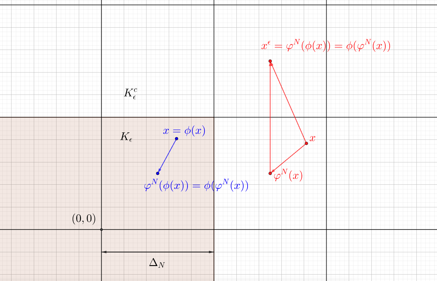
Figure 3: Visualization of $\varphi^{N}\circ\phi=\phi\circ\varphi^{N}$.

We choose $x^{\epsilon}=(2^{j_{\epsilon}}+\frac{1}{m},\dots,2^{j_{\epsilon}}+\frac{1}{m})$ (resp. $x^{\epsilon}=(2^{j_{\epsilon}}+\frac{2^{j_{\epsilon}-1}}{m},\dots,2^{j_{\epsilon}}+\frac{2^{j_{\epsilon}-1}}{m})$) in the case of uniform (resp. non-uniform) grid, where $m=\lceil\frac{1}{\Delta_{N}}\rceil$, see Figure 3. Therefore, we have

$$\left\{\begin{aligned} &\|\phi(x)\|=\|x\|\leq 2T\sqrt{d}\|x\|,\quad&x\in K_{\epsilon}\\ &\|\phi(x)\|=\|x^{\epsilon}\|\leq T\sqrt{d}\,\frac{2^{j}+\frac{2^{j-1}}{m}}{2^{j}}\|x\|\leq 2T\sqrt{d}\|x\|,\quad&x\in K_{\epsilon}^{c}\end{aligned}\right..$$

Together with (83), this yields

$$\mathcal{AW}(\mu,\nu)\leq\int_{K_{\epsilon}^{c}}{\color[rgb]{0,0,0}(1+2T\sqrt{d})}\|x\|\mu(dx)\leq{\color[rgb]{0,0,0}(1+2T\sqrt{d})}\epsilon.$$ (84)

By the triangle equality, we see that

$$\mathcal{AW}(\mu,\bar{\mu}^{N})\leq\mathcal{AW}(\mu,\nu)+\mathcal{AW}(\nu,\bar{\nu}^{N})+\mathcal{AW}(\bar{\mu}^{N},\bar{\nu}^{N}).$$ (85)

Since $\mathcal{AW}(\mu,\nu)$ and $\mathcal{AW}(\nu,\bar{\nu}^{N})$ are already estimated, the only term that remains to be estimated is $\mathcal{AW}(\bar{\mu}^{N},\bar{\nu}^{N})$. For this purpose, we next define a bi-causal coupling $\tilde{\pi}$ between $\bar{\mu}^{N}_{1}$ and $\bar{\nu}^{N}_{1}$. Notice that $\bar{\mu}^{N}=\varphi^{N}_{\#}\mu^{N}$ and $\bar{\nu}^{N}=\varphi^{N}_{\#}\phi_{\#}\mu^{N}$. By choosing $R_{\epsilon}$ to match the boundary of the grid s.t. $\phi\circ\varphi^{N}=\varphi^{N}\circ\phi$, we have $\bar{\nu}^{N}=\phi_{\#}\varphi^{N}_{\#}\mu^{N}=\phi_{\#}\bar{\mu}^{N}$, see Figure 3. So, by the same argument used above, we have that $\tilde{\pi}=(\mathbf{id},\phi)_{\#}\bar{\mu}^{N}\in\text{Cpl}_{\text{bc}}(\bar{\mu}^{N},\bar{\nu}^{N})$. Therefore, by the definition of adapted Wasserstein distance,

$$\begin{split}\mathcal{AW}(\bar{\mu}^{N},\bar{\nu}^{N})&\leq\int\|\varphi^{N}(x)-\varphi^{N}\circ\phi(x)\|\mu^{N}(dx)=\int_{K_{\epsilon}^{c}}\|\varphi^{N}(x)-\varphi^{N}\circ\phi(x)\|\mu^{N}(dx)\quad(\phi|_{K_{\epsilon}}=\mathbf{id})\\ &\leq\int_{K_{\epsilon}^{c}}\big{(}\|\varphi^{N}(x)\|+\|\varphi^{N}(x^{\epsilon})\|\big{)}\mu^{N}(dx)=\int_{K_{\epsilon}^{c}}\big{(}\|\varphi^{N}(x)\|+\|x^{\epsilon}\|\big{)}\mu^{N}(dx)\\ &\leq\int_{K_{\epsilon}^{c}}{\color[rgb]{0,0,0}(1+2T\sqrt{d})}\|\varphi^{N}(x)\|\mu^{N}(dx)={\color[rgb]{0,0,0}(1+2T\sqrt{d})}\int_{K_{\epsilon}^{c}}\|x\|\bar{\mu}^{N}(dx).\end{split}$$ (86)

Step 2: Now we claim that

$$\begin{split}\limsup_{N\to\infty}\int_{K_{\epsilon}^{c}}\|x\|\bar{\mu}^{N}(dx)\leq\limsup_{N\to\infty}\int_{K_{\epsilon}^{c}}\|x\|\mu^{N}(dx).\end{split}$$ (87)

We are going to prove this separately for the uniform and non-uniform adapted empirical measures.
(i) In the case of uniform adapted empirical measure, for all $x\in\mathbb{R}^{dT}$ we have $\|\hat{\varphi}^{N}(x)-x\|\leq T\sqrt{d}\Delta_{N}$. Thus, we obtain that

$$\limsup_{N\to\infty}\int_{K_{\epsilon}^{c}}\|x\|\hat{\mu}^{N}(dx)\leq\limsup_{N\to\infty}\Big{(}\int_{K_{\epsilon}^{c}}\|x\|\mu^{N}(dx)+T\sqrt{d}\Delta_{N}\Big{)}=\limsup_{N\to\infty}\int_{K_{\epsilon}^{c}}\|x\|\mu^{N}(dx).$$ (88)

(ii) In the case of non-uniform adapted empirical measure, for all $j\in\mathbb{N}$ and $x\in\mathcal{A}_{j}$ we have $\|\check{\varphi}^{N}(x)-x\|\leq T\sqrt{d}\Delta_{N}2^{j}$. Thus, we obtain that

$$\int_{K_{\epsilon}^{c}}\|x\|\check{\mu}^{N}(dx) =\sum_{j=0}^{\infty}\int_{\mathcal{A}_{j}\cap K_{\epsilon}^{c}}\|\check{\varphi}^{N}(x)\|\mu^{N}(dx)\leq\sum_{j=0}^{\infty}\int_{\mathcal{A}_{j}\cap K_{\epsilon}^{c}}\big{(}\|\check{\varphi}^{N}(x)-x\|+\|x\|\big{)}\mu^{N}(dx)$$

$$\leq T\sqrt{d}\sum_{j=0}^{\infty}2^{j}\Delta_{N}\mu^{N}(\mathcal{A}_{j}\cap K_{\epsilon}^{c})+\int_{K_{\epsilon}^{c}}\|x\|\mu^{N}(dx)$$

$$=T\sqrt{d}\Delta_{N}+2T\sqrt{d}\Delta_{N}\sum_{j=1}^{\infty}2^{j-1}\mu^{N}(\mathcal{A}_{j}\cap K_{\epsilon}^{c})+\int_{K_{\epsilon}^{c}}\|x\|\mu^{N}(dx),~{}\text{(Since for all $x\in\mathcal{A}_{j}$, $\|x\|\geq 2^{j-1}$)}$$

$$\leq T\sqrt{d}\Delta_{N}+2T\sqrt{d}\Delta_{N}\sum_{j=1}^{\infty}\int_{\mathcal{A}_{j}\cap K_{\epsilon}^{c}}\|x\|\mu^{N}(dx)+\int_{K_{\epsilon}^{c}}\|x\|\mu^{N}(dx)$$

$$=T\sqrt{d}\Delta_{N}+(2T\sqrt{d}\Delta_{N}+1)\int_{K_{\epsilon}^{c}}\|x\|\mu^{N}(dx).$$

By letting $N\to\infty$, $\Delta_{N}\to 0$ and we get

$$\limsup_{N\to\infty}\int_{K_{\epsilon}^{c}}\|x\|\check{\mu}^{N}(dx)\leq\limsup_{N\to\infty}\int_{K_{\epsilon}^{c}}\|x\|\mu^{N}(dx).$$

This combined with (88) completes the proof of the claim (87).
Step 3: Recall that $\mu$ is integrable by assumption. Then, by the law of large numbers,

$$\begin{split}\lim_{N\to\infty}\int_{K_{\epsilon}^{c}}\|x\|\mu^{N}(dx)=\int_{K_{\epsilon}^{c}}\|x\|\mu(dx)\leq\epsilon.\end{split}$$ (89)

Therefore, combining (86), (87) and (89), we have that

$$\limsup_{N\to\infty}\mathcal{AW}(\bar{\mu}^{N},\bar{\nu}^{N})\leq{\color[rgb]{0,0,0}(1+2T\sqrt{d})}\epsilon.$$ (90)

Finally, combining (82), (84), (85) and (90), we conclude that

$$\limsup_{N\to\infty}\mathcal{AW}(\mu,\bar{\mu}^{N})\leq\limsup_{N\to\infty}\Big{(}\mathcal{AW}(\mu,\nu)+\mathcal{AW}(\nu,\bar{\nu}^{N})+\mathcal{AW}(\bar{\mu}^{N},\bar{\nu}^{N})\Big{)}\leq{\color[rgb]{0,0,0}(2+4T\sqrt{d})}\epsilon.$$

We then let $\epsilon\to 0$ and complete the proof of Theorem 2.7. ∎

References

• [ABZ20] Beatrice Acciaio, Julio Backhoff-Veraguas and Anastasiia Zalashko “Causal optimal transport and its links to enlargement of filtrations and continuous-time stochastic optimization” In Stochastic Processes and their Applications 130.5 Elsevier, 2020, pp. 2918–2953
• [AL18] Jonas Adler and Sebastian Lunz “Banach wasserstein gan” In Advances in Neural Information Processing Systems 31, 2018
• [Bac+17] Julio Backhoff-Veraguas, Mathias Beiglbock, Yiqing Lin and Anastasiia Zalashko “Causal transport in discrete time and applications” In SIAM Journal on Optimization 27.4 SIAM, 2017, pp. 2528–2562
• [Bac+20] Julio Backhoff-Veraguas, Daniel Bartl, Mathias Beiglböck and Manu Eder “Adapted Wasserstein distances and stability in mathematical finance” In Finance and Stochastics 24 Springer, 2020, pp. 601–632
• [Bac+22] Julio Backhoff-Veraguas, Daniel Bartl, Mathias Beiglböck and Johannes Wiesel “Estimating processes in adapted Wasserstein distance” In The Annals of Applied Probability 32.1 Institute of Mathematical Statistics, 2022, pp. 529–550
• [BT19] Jocelyne Bion–Nadal and Denis Talay “On a Wasserstein-type distance between solutions to stochastic differential equations” In The Annals of Applied Probability 29.3 Institute of Mathematical Statistics, 2019, pp. 1609–1639
• [Boi11] Emmanuel Boissard “Simple bounds for the convergence of empirical and occupation measures in 1-Wasserstein distance” In Electronic Journal of Probability 16 Institute of Mathematical StatisticsBernoulli Society, 2011, pp. 2296–2333
• [BL14] Emmanuel Boissard and Thibaut Le Gouic “On the mean speed of convergence of empirical and occupation measures in Wasserstein distance” In Annales de l’IHP Probabilités et statistiques 50.2, 2014, pp. 539–563
• [BGV07] François Bolley, Arnaud Guillin and Cédric Villani “Quantitative concentration inequalities for empirical measures on non-compact spaces” In Probability Theory and Related Fields 137.3 Springer, 2007, pp. 541–593
• [BY78] Pierre Brémaud and Marc Yor “Changes of filtrations and of probability measures” In Zeitschrift für Wahrscheinlichkeitstheorie und verwandte Gebiete 45.4 Springer, 1978, pp. 269–295
• [DF15] Jérôme Dedecker and Xiequan Fan “Deviation inequalities for separately Lipschitz functionals of iterated random functions” In Stochastic Processes and their Applications 125.1 Elsevier, 2015, pp. 60–90
• [DSS13] Steffen Dereich, Michael Scheutzow and Reik Schottstedt “Constructive quantization: Approximation by empirical measures” In Annales de l’IHP Probabilités et statistiques 49, 2013, pp. 1183–1203
• [FG15] Nicolas Fournier and Arnaud Guillin “On the rate of convergence in Wasserstein distance of the empirical measure” In Probability Theory and Related Fields 162.3 Springer, 2015, pp. 707–738
• [Gig08] Nicola Gigli “On the geometry of the space of probability measures in Rn endowed with the quadratic optimal transport distance”, 2008
• [GPP19] Martin Glanzer, Georg Ch Pflug and Alois Pichler “Incorporating statistical model error into the calculation of acceptability prices of contingent claims” In Mathematical Programming 174.1 Springer, 2019, pp. 499–524
• [GL07] Nathael Gozlan and Christian Léonard “A large deviation approach to some transportation cost inequalities” In Probability Theory and Related Fields 139.1 Springer, 2007, pp. 235–283
• [Han22] Bing Han “Distributionally robust risk evaluation with causality constraint and structural information”, 2022
• [IS98] Rustam Ibragimov and Sh Sharakhmetov “On an exact constant for the Rosenthal inequality” In Theory of Probability & Its Applications 42.2 SIAM, 1998, pp. 294–302
• [IS01] Rustam Ibragimov and Sh Sharakhmetov “The best constant in the Rosenthal inequality for nonnegative random variables” In Statistics & probability letters 55.4 Elsevier, 2001, pp. 367–376
• [Kle+22] Konstantin Klemmer, Tianlin Xu, Beatrice Acciaio and Daniel B. Neill “SPATE-GAN: Improved Generative Modeling of Dynamic Spatio-Temporal Patterns with an Autoregressive Embedding Loss” In AAAI, 2022
• [Las18] Rémi Lassalle “Causal transference plans and their Monge-Kantorovich problems” In Stochastic Processes and their Applications 36.3 Elsevier, 2018, pp. 452–484
• [Lei20] Jing Lei “Convergence and concentration of empirical measures under Wasserstein distance in unbounded functional spaces” In Bernoulli 26.1 Bernoulli Society for Mathematical StatisticsProbability, 2020, pp. 767–798
• [McD89] Colin McDiarmid “On the method of bounded differences” In Surveys in combinatorics 141.1 Norwich, 1989, pp. 148–188
• [OW21] Jan Obłój and Johannes Wiesel “Robust Estimation of Superhedging Prices” In Derivatives eJournal, 2021
• [PP12] Georg Ch Pflug and Alois Pichler “A distance for multistage stochastic optimization models” In SIAM Journal on Optimization 22.1 SIAM, 2012, pp. 1–23
• [PP14] Georg Ch Pflug and Alois Pichler “Multistage stochastic optimization” Springer, 2014
• [PP15] Georg Ch Pflug and Alois Pichler “Dynamic generation of scenario trees” In Computational Optimization and Applications 62.3 Springer, 2015, pp. 641–668
• [PP16] Georg Ch Pflug and Alois Pichler “From empirical observations to tree models for stochastic optimization: convergence properties” In SIAM Journal on Optimization 26.3 SIAM, 2016, pp. 1715–1740
• [Pic13] Alois Pichler “Evaluations of risk measures for different probability measures” In SIAM Journal on Optimization 23.1 SIAM, 2013, pp. 530–551
• [Rüs85] Ludger Rüschendorf “The Wasserstein distance and approximation theorems” In Probability Theory and Related Fields 70.1 Springer, 1985, pp. 117–129
• [Ver18] Roman Vershynin “High-dimensional probability: An introduction with applications in data science” Cambridge university press, 2018
• [Wie22] Johannes Wiesel “Measuring association with Wasserstein distances” In Bernoulli, 2022
• [Xu+20] Tianlin Xu, Li Kevin Wenliang, Michael Munn and Beatrice Acciaio “COT-GAN: Generating Sequential Data via Causal Optimal Transport” In ArXiv abs/2006.08571, 2020