Optimal service station design for traffic mitigation via genetic algorithm and neural network

Abstract

This paper analyzes how the presence of service stations on highways affects traffic congestion. We focus on the problem of optimally designing a service station to achieve beneficial effects in terms of total traffic congestion and peak traffic reduction. Microsimulators cannot be used for this task due to their computational inefficiency. We propose a genetic algorithm based on the recently proposed Cell Transmission Model with service station (CTM-s), that efficiently describes the dynamics of a service station. Then, we leverage the algorithm to train a neural network capable of solving the same problem, avoiding implementing the CTM-s. Finally, we examine two case studies to validate the capabilities and performance of our algorithms. In these simulations, we use real data extracted from Dutch highways.

1 Introduction

During the last decades, traffic congestion has been worsening in major cities around the world creating costs not only in terms of waiting for resources but also in terms of emissions. According to the INRIX $2021$ Global Traffic Scorecard report, the U.S. drivers wasted on average $99$ hours a year due to traffic congestion, generating nearly $\$88$ billion in total costs. The situation was even worse in France, where in $2021$ drivers in Paris spent on average 140 hours in traffic INRIX (2022).

To manage rush hour traffic, a wide variety of tools have been proposed in the literature as well as implemented in practice. Arguably, one of the most effective approaches is the optimal design of the traffic infrastructure with the goal of mitigating the traffic congestion. On highways, an important factor influencing the flow of vehicles is the presence of Service Stations (STs). Initially, authors focused on the modelling and optimally control of ST by employing queuing theory, see (Wang and Huang, 1995). More recently, the spread of electric vehicles renew the interest of the research community towards service stations, and in particular those offering the possibility to recharge Plug-in Electric Vehicle (PEV). Ferro et al. (2020) propose a bi-level where the higher level aims at computing the optimal planning of charging stations. The lower level instead is modelled as a traffic assignment problem among commuters. The problem of finding the optimal location of charging stations has been also studied in (Kong et al., 2017, 2019), where the authors consider a simple traffic model interconnected with the power grid to determine where the charging station should be located. Refer to (Pagany et al., 2019) for a survey on spatial localization methodologies for the PEV charging infrastructure.

In (Gusrialdi et al., 2017), the authors propose a control scheme to mitigate queues at charging stations optimizing the drivers experience. An incentive based control is presented in (Cenedese et al., 2022b), where a dynamic discount on the charging of PEV is able to decrease traffic congestion over a bottleneck. Finally, in (Cenedese et al., 2021), the authors incentivize electric vehicles to stop at a ST during periods of peak congestion via a discount on the purchased energy. This is an online control of a ST base on game theory (similarly to (Cenedese et al., 2019)) and it is able to decrease the peak of traffic congestion.

The majority of the contributions in the literature focuses more on charging stations rather than the more general STs. Moreover, they do not consider the effect that such stations have on the mainstream traffic dynamics and the possibility that a careful design can mitigate traffic congestion. In this work, we bridge this gap formulating the problem of optimal design of a ST with the objective of minimizing the overall traffic congestion. The main contribution of the paper can be summarized as follows:

• we formalize the problem of the optimal design of a ST to mitigate traffic congestion using the CTM-s as a Mixed Integer Nonlinear Programming (MI-NLP);

• we design a Genetic Algorithm (GA) able to compute the optimal solution of the MI-NLP for a given highway stretch;

• we use the GA to create a training dataset for different highways configurations and use it to train a Neural Network (NN). Once trained, the NN is able to solve the problem without requiring the user to implement the CTM-s;

• we analyze two case studies based on real data and validate the efficacy of the proposed solutions.

2 Problem formulation

Figure 1: The model and variables of the CTM-s, including on- and off-ramps together with a single ST $(i,j)$.

In this section, we first propose a brief introduction on the CTM-s and discuss the variables involved in the optimal design of a service station. Then, we formalize the problem as a general MI-NLP.

2.1 CTM-s overview

The CTM-s was recently proposed by Cenedese et al. (2022a) as an extension of the classical Cell Transmission Model (CTM) (see e.g. (Daganzo, 1992)), where a highway stretch is divided into $N$ consecutive cells described by the index set $\mathcal{N}\coloneqq\{1,\cdots,N\}$. If a driver can enter a ST from cell $i$, called access cell, and exit it by merging back into the mainstream in cell $j$, called exit cell, then the ST is denoted by the ordered couple $p=(i,j)\in\mathcal{M}\subseteq\mathcal{N}\times\mathcal{N}$, see Figure 1. The cardinality of the set describes the number of service stations, i.e., $M=|\mathcal{M}|$. In this work, we focus on the optimal design of a single unimodal ST on a highway stretch, i.e., $M=1$ and the drivers at the ST are assumed to be homogeneous. This standing assumptions simplify some of the dynamics introduced in (Cenedese et al., 2022a, Sec. II.A). Relaxing these assumptions would not create technical difficulties but rather increase the computational complexity of the problem, and thus it is left for future works.

The intrinsic characteristics of the highway stretch are described by the set of parameters in Table 1. To facilitate the discussion, we distinguish the parameters in three different groups according to the type: those associated with the cells (denoted by $P$), those describing the ST (denoted by $S$), and finally some other parameter that is assumed to be fixed (denoted by $F$). More precisely, we define the first two types by the following vectors

$$P=\mathrm{col}((L_{i},\overline{v}_{i},q_{i}^{\max},\rho_{i}^{\max},\beta_{i})_{i\in\mathcal{N}})\in\mathbb{R}^{6N}$$

and

$$S=\mathrm{col}(i,j,\delta_{(i,j)},\beta^{\textup{s}}_{i})\in\mathcal{S}=\mathcal{N}^{2}\times\mathbb{R}\times[0,1].$$

The values of the parameters in $F$ are the result of a reasonable design choice on the ST.

Table 1: CTM-s parameters associated with cell $i\in\mathcal{N}$ and ST $p=(i,j)$ divided by type: $P$, $S$, or $F$.

	Name	Unit	Description
$P$	$L_{i}$	[km]	cell length
	$\overline{v}_{i}$	[km/h]	free-flow speed
	$w_{i}$	$[\textup{km/h}]$	congestion wave speed
	$q_{i}^{\max}$	$[\textup{veh/h}]$	maximum cell capacity
	$\rho_{i}^{\max}$	$[\textup{veh/km}]$	maximum jam density
	$\beta_{i}$	%	off-ramp split ratio
$S$	$i$		ST’s access cell
	$j$		ST’s exit cell
	$\delta_{(i,j)}$	[h]	avg. time spent at the ST
	$\beta^{\textup{s}}_{i}$	%	ST’s off-ramp split ratio
$F$	$p_{i}^{\textup{ms}}$		priority of mainstream $i$
	$r^{\textup{s},\max}_{j}$	$[\textup{veh/h}]$	ST’s maximum on-ramp capacity
	$L_{(i,j)}$		ST’s length in number of cells

The traffic flow dynamics evolve over $T_{\textup{h}}$ time intervals $k$ of length $T$ and indexed by the set $\mathcal{T}\coloneqq\{1,\cdots,T_{\textup{h}}\}$. The mainstream and ST dynamics are described via the CTM-s variables listed in Table 2. The density $\rho_{i}$ of cell $i$ is described by

$$\rho_{i}(k+1)=\rho_{i}(k)+\dfrac{T}{L_{i}}\left(\Phi_{i}^{+}(k)-\Phi_{i}^{-}(k)\right)\>,$$ (1)

where the inflow and outflow are defined respectively as

$$\Phi^{-}_{i}(k) =\phi_{i+1}(k)+s_{i}(k)+s^{\textup{s}}_{i}(k)$$ (2a)

$$\Phi^{+}_{i}(k) =\phi_{i}(k)+r_{i}(k)+r^{\textup{s}}_{i}(k).$$ (2b)

Note that throughout the paper we consider $\phi_{1}(k)$ and the demand of the on-ramps as known external inputs to the dynamical system.

The flow of vehicles entering the ST and exiting the highway via an off-ramp from cell $i$ are simply defined via the associated splitting ratios, i.e., $s^{\textup{s}}_{i}(k)=\beta^{\textup{s}}_{i}\Phi^{-}_{i}(k)$ and $s_{i}(k)=\beta_{i}\Phi^{-}_{i}(k)$ where $\beta^{\textup{s}}_{i}+\beta_{i}\leq 1$.

Table 2: CTM-s variables for the dynamics at time $k\in\mathbb{N}$ associated with cell $i\in\mathcal{N}$ and ST $p=(i,j)$.

Name	Unit	Description
$\rho_{i}(k)$	$[\textup{veh/km}]$	traffic density of cell $i$
$\Phi_{i}^{+}(k)(\Phi_{i}^{-}(k))$	$[\textup{veh/h}]$	total flow entering (exiting) cell $i$
$\phi_{i}(k)$	$[\textup{veh/h}]$	flow entering cell $i$ from $i-1$
$r_{i}(k)$	$[\textup{veh/h}]$	flow merging into $i$ via an on-ramp
$s_{i}(k)$	$[\textup{veh/h}]$	flow leaving $i$ via an off-ramp
$\ell_{(i,j)}(k)$	$\>[\textup{veh}]$	vehicles currently at the ST
$e_{(i,j)}(k)$	$\>[\textup{veh}]$	vehicles queuing to exit the ST
$s^{\textup{s}}_{i}(k)$	$[\textup{veh/h}]$	flow leaving $i$ to enter the ST
$r^{\textup{s}}_{j}(k)$	$[\textup{veh/h}]$	flow merging into $j$ from the ST

The dynamics of the ST $p=(i,j)$ are described by: the number of vehicles at the ST during the time interval $k$, i.e.,

$$\ell_{p}(k+1)=\ell_{p}(k)+T\left[s_{i}^{\textup{s}}(k)-r^{\textup{s}}_{j}(k)\right],$$ (3)

and among the vehicles at the ST, by the ones waiting for merging back into the mainstream, i.e.,

$$e_{p}(k+1)=e_{p}(k)+T\left[s_{i}^{\textup{s}}(k-\delta_{p})-r^{\textup{s}}_{j}(k)\right]\,.$$ (4)

The number of vehicles that attempt to exit the ST during $k$ is $s^{\textup{s}}_{i}(k-\delta_{p})+\frac{e_{p}(k)}{T}$, while the demand of vehicles that try to merge back into the mainstream reads as

$$D^{\textup{s}}_{p}(k)=\min\left(s^{\textup{s}}_{i}(k-\delta_{p})+\frac{e_{p}(k)}{T},r_{j}^{\textup{s},\max}\right).$$ (5)

Due to space limitations, we omit the rest of the dynamics derivation that can be found in (Cenedese et al., 2022a, Eq. 7-14), i.e, the exact definitions of the demand and supply among cells in the case of free-flow and congested scenarios that in turn are used to compute $\phi_{i}(k)$ and $r^{\textup{s}}_{i}(k)$, respectively.

By denoting all the CTM-s variables in Table 2 as $x$, we define the dynamics of the whole model in compact form as

$$x(k+1)=f(x(k),S,P,F),$$ (6)

where $f$ is a highly nonlinear parametric function that incorporate the dynamics in (1)–(5) and (Cenedese et al., 2022a, Eq. 7-14). The dependency from $\phi_{1}$ and the demand of the on-ramps have been omitted to ease the notation.

2.2 General MI-NLP formulation

In this section, we formalize the problem of optimal ST design and cast it as a MI-NLP.

2.2.1 Cost function:

We are now ready to elaborate the concept of optimality considered in this work. As previously stated, the effect that a ST has on the traffic conditions is relevant and thus its design can alleviate or exacerbate the traffic congestion on the highway stretch. To quantify such effect, we introduce two cost components, i.e., $\xi_{\Delta}$ and $\pi_{\Delta}$, which are both related to the additional travel time due to the traffic congestion on the highway stretch during $k\in\mathcal{T}$, i.e.,

$$\Delta(k)\coloneqq\sum_{i\in\mathcal{N}}\left(\dfrac{L_{i}}{v_{i}(k)}-\dfrac{L_{i}}{\overline{v}_{i}}\right)\in\mathbb{R}_{+}.$$ (7)

Notice that $\Delta(k)=0$ implies that the highway is operating in free-flow conditions.

The first cost component corresponds to the area under $\Delta$, hence

$$\xi_{\Delta}(S|P)=T\sum_{k\in\mathcal{T}}\Delta(k)\in\mathbb{R}_{+},$$ (8)

and it captures an aggregate information on the duration and intensity of the traffic congestion. From (7), it follows that if $\xi_{\Delta}=0$, then there is no congestion during $\mathcal{T}$. This quantity is a non-normalized version of the Relative Congestion Index (RCI) used in (Afrin and Yodo, 2020; Tang and Heinimann, 2018).

On top of minimizing $\xi_{\Delta}$, we also aim at achieving a peak-shaving effect on the traffic congestion. For this reason the second cost component captures the percentage of peak congestion reduction due to the (beneficial) presence of the ST, and it is defined as follows

$$\pi_{\Delta}(S|P)=\dfrac{\max_{k}(\Delta_{0}(k))-\max_{k}(\Delta(k))}{\max_{k}(\Delta_{0}(k))}\leq 1,$$ (9)

where $\Delta_{0}$ is computed as in (7), considering no ST on the highway stretch. Here, $\pi_{\Delta}=1$ implies that there is a complete elimination of the peak, i.e., the highway operates in free-flow conditions. On the other hand, if $\pi_{\Delta}\leq 0$ there is no beneficial effect in introducing the ST in terms of peak reduction.

Then, the final cost function used in the optimization problem reads as

$$c(S|P)=\alpha\xi_{\Delta}(S|P)-\pi_{\Delta}(S|P),$$ (10)

where $\alpha$ is a normalizing coefficient. Specifically, if $\alpha=1/(\sum_{i}{\textstyle\frac{L_{i}}{\overline{v}_{i}}})$, then the first component of $c$ corresponds to the RCI.

2.2.2 Constraints:

The choice of the feasible ST’s parameters $S$ is limited by a set of constraints that are necessary to ensure that the attained results have a clear physical interpretation. In the remainder, given a vector $y$, we denote its $q$-th component by $[y]_{q}$.

First, we ensure that the length of the ST is exactly equal to $L_{(i,j)}$. Then, the parameters $S\in\mathcal{S}$ must satisfy

$$[S]_{2}-[S]_{1}=L_{(i,j)}.$$ (11)

The rest are box constraints limiting the values of $S$. We can describe in compact form all the above constraints as $AS\leq b$, for a suitable choice of $A$ and $b$.

Remark 1

Given the particular configuration of the highways or preferences, different constraints can be added. For example, the access point of the ST can be constrained to be only in those cells that do not already have a on- or off-ramp.

We are now ready for formulating the problem of designing the optimal ST for a highway stretch associated with a specific $P$, i.e., computing $S^{\star}$ by solving the following MI-NLP problem

$$S^{\star}= \operatorname*{argmin}_{S\in\mathcal{S}} c(S|P)$$ (12)

s.t. $$AS\leq b$$

$$x(k+1)=f(x(k),S,P,F),\>\forall k\in\mathcal{T}$$

$$x(0)=x_{0},$$

where $x_{0}$ are the dynamics’ initial conditions. The presence of integer variables in $S$ (the first two components) and the highly nonlinar dynamics of the CTM-s with respect to $S$ make the problem complex from both a theoretical and computational point of view. Although approximations that simplify the classical CTM dynamics have been proposed in (Ziliaskopoulos, 2000; Lo, 2001), these modifications do not simplify much problem (12) since the optimization is performed with respect to $S$.

3 Genetic Algorithm

The first solution we present is based on the GA that has been successfully applied in the past also by other authors working on traffic control to attain numerical solutions to “untractable” optimization problems, see (Lo et al., 2001).

The structure of the GA is simple and very effective. First, a set of candidate maximizers of a given fitness function are selected, then their fitness is computed, and finally a new “generation” of candidates is obtained by creating variations of the best performing ones, refer to (Katoch et al., 2021) for an a detailed overview on the topic.

The first population $\mathfrak{S}_{1}$ is composed of $N_{\textup{GA}}$ candidates randomly chosen in the set of feasible design parameters, that is

$$\left\{S\in\mathcal{S}\,|\,AS\leq b\right\}.$$ (13)

The fitness function is simply the opposite of the cost in (10), hence, for a given $(P,F)$ and $x_{0}$, the fitness of $S\in\mathfrak{S}_{i}$ in generation $i$ is $-c(S|P)$.

Given a generation $j$ and the set of $N_{\textup{GA}}^{\star}\leq N_{\textup{GA}}$ best performing elements $\mathfrak{S}_{j}^{\star}\subseteq\mathfrak{S}_{j}$, the new population $\mathfrak{S}_{j+1}$ includes the $N_{\textup{GA}}^{\star}$ best performing elements of generation $j$, i.e., $\mathfrak{S}_{j}^{\star}$, and also their offspring and mutations. The offspring exploits the best performers of the previous generation, i.e., $\mathfrak{S}_{j}^{\star}$ and are generated via double-point crossover. On the other hand, the mutations, chosen randomly, make the GA explore the space of feasible parameters in (13), reducing the probability of converging to local minima. In $\mathfrak{S}_{j+1}$, $N_{\textup{GA}}-N_{\textup{GA}}^{\star}$ elements are composed by the offspring and mutations, and among these the probability of mutation is denoted by $p_{\textup{GA}}$. Note that in general we cannot guarantee that the new elements satisfy the constraints. Then, this issue can be overcome in two ways: the unfeasible solutions are replaced by new feasible ones, or a very low fit can be assigned to unfeasible solutions such that the algorithm is forced to not select them. The GA stops when the number of contiguous generations with no improvement of the fitness exceeds $K_{\textup{stop}}$.

3.1 Implementation

We validate the discussed GA by comparing it with a “brute force” algorithm that solves (12) by sampling the set of feasible $S$ and find the optimal solution by inspection. Due to the combinatorial nature of the brute force algorithm, we consider highway stretches with a moderate number of cells and we perform a moderate number of comparison between the two algorithms. Namely, we use 5 different choices of $P$ for $N\in\{10,15,20\}$ attaining a total number of 15 different values of $P$ used to validate the GA. As expected, the brute force algorithm computational time grows rapidly with $N$, see Table 3.

Table 3: Execution time

N	$10$	$15$	$20$
avg. time brute force	$1.39$ [h]	$2.26$ [h]	$3.14$ [h]
avg. time GA	$0.13$ [h]	$0.31$ [h]	$0.42$ [h]

We denote this validation set by $\mathfrak{P}$; the parameters of each cell composing $P\in\mathfrak{P}$ are randomly selected within the intervals in Table 4. The selected values are in line with those identified in the case study presented in Section 5. The value of $\alpha$ has been chosen equal to $0.01$.

Figure 2: Input $\phi_{1}(k)$ used for the simulations.

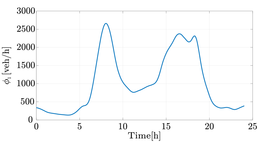
The value of $\phi_{1}(k)$ in Figure 2 is used for all the simulations, and it is a smooth version of the flow in a highway line during a typical working day. Here, we considered highway stretches in which there are no on- and off-ramps. As anticipated, the values of $F$ has been considered fixed and equal to

$$F=\mathrm{col}(0.95,\,1500,\,2).$$ (14)

Table 4: Range of values used to generate the different $P\in\mathfrak{P}$.

$L_{i}$[m]	$\overline{v}_{i}$ [km/h]	$w_{i}$[km/h]	$q_{i}^{\max}$ [veh/h]	$\rho_{i}^{\max}$[veh/km]
$[300,1000]$	$[80,110]$	$[10,40]$	$[1500,2500]$	$[70,100]$

We implemented the GA in Python using the PyGAD, the parameters of the algorithm are reported in Table 5. The GA’s parameters are kept constant for all $P\in\mathfrak{P}$.

Table 5: GA parameters

$N_{\textup{GA}}$	$N_{\textup{GA}}^{\star}$	$p_{\textup{GA}}$	$K_{\textup{stop}}$
16	4	0.1	7

The range of values from which the components of $S\in\mathfrak{S}_{1}$ are randomly drawn are reported in Table 6, the same intervals are used as upper and lower bounds constraints for all $S\in\mathfrak{S}_{j}$ and $j\in\mathbb{N}$.

Table 6: Range of values for $S\in\mathfrak{S}_{j}$ and $j\in\mathbb{N}$.

$(i,j)$	$\delta_{(i,j)}$ [min]	$\beta^{\textup{s}}_{i}$
$\mathcal{N}\times\mathcal{N}$	$[0,720]$	$[0,\,0.2]$

Figure 3: Fitness of the best performing $S\in\mathfrak{S}_{j}$ for each generation $j$. The plateau after generation $25$ is where we identify $S^{\star}$.

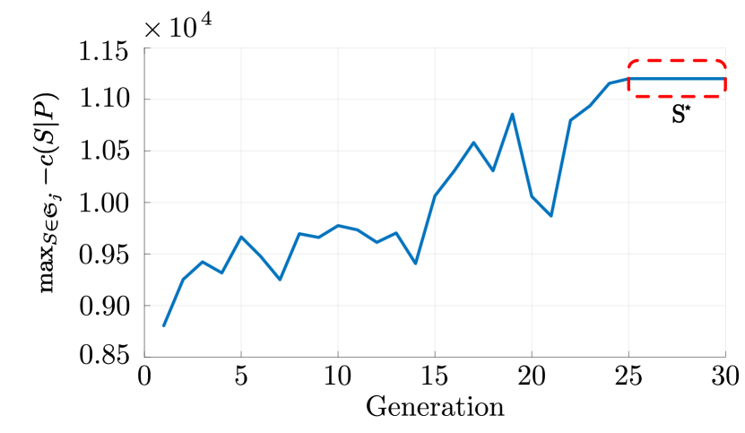
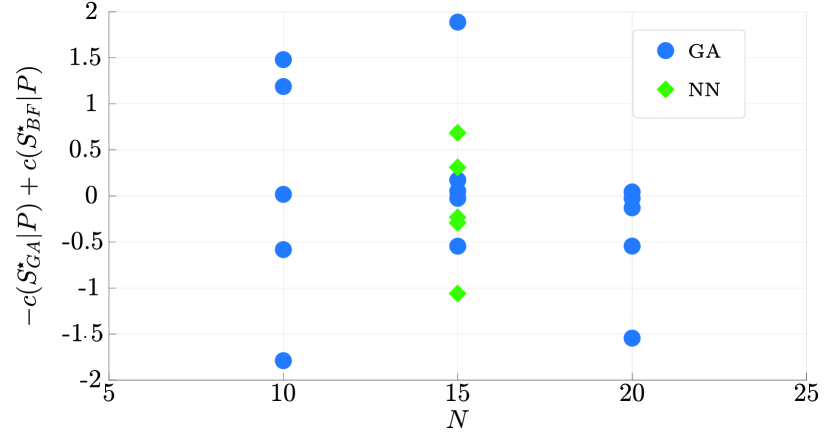
As shown in Figure 3, the GA takes only $30$ generations to converge to $S^{\star}_{\textup{GA}}$. We compare the cost $S^{\star}_{\textup{GA}}$ with the one achieved by the brute force solution $S^{\star}_{\textup{BF}}$. In Figure 4, we plot for all $P\in\mathfrak{P}$ the difference $c(S^{\star}_{\textup{BF}}|P)-c(S^{\star}_{\textup{GA}}|P)$. The result obtained by the GA is comparable to the one obtained via the brute force algorithm. In fact, the difference between the two values stays in the interval $[-2,2]$ even though the cost is usually on the order of hundreds. Therefore, the GA can successfully compute a solution to (12) that achieves performance similar to those attained via the brute force algorithm. Interestingly, in some circumstances $S^{\star}_{\textup{GA}}$ obtains a lower cost than the one obtained by $S^{\star}_{\textup{BF}}$. This is due to the sampling on the feasible space of $S$ that in some circumstances is not dense enough.

Figure 4: The difference between the maximum fitness value computed via the brute force algorithm and the one attained via GA (in blue) and via NN (in blue) for different values of $P\in\mathfrak{P}$.

4 Neural Network

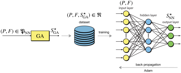
One of the drawbacks of the GA is its lack of scalability when the length and complexity of the stretches increase. Moreover, it highly depends on the underlying model, i.e. the CTM-s, and it solves (12) for one specific stretch, i.e., $P$. In this section, we aim at tackling these shortcomings by deriving an approximation of the mapping between the features of a generic highway stretch ($P$ and $F$), and the associated $S^{\star}$. We achieve this via a NN that requires a single computationally expansive training session but after that it can be used with negligible computational time for generic stretches, refer to (Hagan et al., 1997; Abiodun et al., 2018) and references therein.

To train the NN, we need an extensive dataset of different highways stretches and optimal ST. Real data cannot be used since the location of the ST cannot be changed and thus it cannot be assessed whether it is the optimal choice or not. An alternative can be represented by microsimulators, such as Aimsun Next 22, that are widely regarded as precise representations of real traffic dynamics. However, the execution times are prohibitive. In fact, a simulation of the $24$ hours on a $6$ km highway stretch require $30$ minutes to be completed. Therefore, finding the optimal ST design and repeat the process to create dataset of reasonable size is practically unfeasible.

The CTM-s represents a novel opportunity, which makes it possible to process over $4\cdot 10^{4}$ days of simulation in less than $24$ hours. Moreover, for each highway stretch, identified by $(P,F)$, we can leverage the GA introduced in the previous section to compute $S^{\star}_{\textup{GA}}$, and thus generate a collection of tuples $(P,F,S^{\star}_{\textup{GA}})$ that compose the training dataset $\mathfrak{N}$, see Figure 5. To create a database that comprehends as many scenarios as possible, we vary not only $P$ but also $F$, within reasonable ranges. The set of all these couples $(P,F)$ is denoted by $\mathfrak{P}_{\textup{NN}}$. The variation of $\phi_{1}(k)$ and, if present, of the on-ramps’ demand should be performed carefully. In fact, the choice of unrealistic demand profiles for a given highway stretch can generate a biased NN.

Our numerical simulations show that a NN with a single hidden layer is able to learn how to solve (12), if the dataset $\mathfrak{N}$ captures enough isntances of the CTM-s dynamics. The input layer is composed of as many layer as the components of $(P,F)$. Notice that this implies that, for highway stretches with different number of cells $N$, different NNs should be trained. The generalisation of the method to relax this assumption is left for future works.

We select Adam (Kingma and Ba, 2014) as backpropagation algorithm. It is an adaptive momentum gradient descent based algorithm able to achieve satisfactory results by dynamically change the learning rate as the learning progresses. Finally, we use the Mean Logarithmic Squared Error (MLSE) as loss function for both the training and validation.

Figure 5: The pipeline used to generate the dataset $\mathfrak{N}$ and train of the NN from the initial set $\mathfrak{S}_{\textup{NN}}$.

4.1 Implementation

Next we derive the NN as described above; for the implementation we use Tensorflow. To training dataset $\mathfrak{N}$ is attaiend from a collection of $|\mathfrak{S}_{\textup{NN}}|=10^{4}$ highway stretches of $N=15$ cells. Each cell’s parameters are randomly drawn from the ranges in Table 7.

Table 7: Range of parameters used to generate $\mathfrak{S}_{\textup{NN}}$ and then $\mathfrak{N}$.

	$|\mathfrak{S}_{\textup{NN}}|$ and $|\mathfrak{N}|$	$10^{4}$
$P$	$L_{i}$	$[300,\,1000]$
	$\overline{v}$	$[80,\,110]$
	$w$	$[10,\,40]$
	$q^{\max}$	$[1500,\,2500]$
	$\rho^{\max}$	$[70,\,100]$
$F$	$p^{\textup{ms}}_{i}$	0.95
	$r^{\textup{s,max}}_{j}$	1500
	$L_{(i,j)}$	$2$

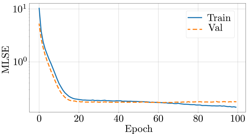
The GA is tuned as in the previous section, i.e., according to Table 5 and 6. For the training phase, we tested different batch sizes, i.e., the number of samples that will be propagated through the NN. Large batches degrade the NN’s ability to generalize while small ones create convergence problems, see Figure 6. The best results are obtained for batches of $[60,70]$ samples, with an MLSE between $0.160$ and $0.162$, showing that the NN is able to compute a solution $S^{\star}_{\textup{NN}}$ that is almost identical to the one obtained via the GA. This is confirmed by Figure 4 where $S^{\star}_{\textup{NN}}$, compared to the brute force solution, obtains similar performance to those of the GA.

Table 8: NN configuration and MLSE values calculate on the validation data set.

Hidden layers	$1$
Neurons hidden layer	$55$
Dropout hidden layer	$0.2$
Activation function	ReLU
Batch size	$[60,\,70]$
Optimizer	Adam
Learning rate	Adaptive

Figure 6: Loss function, i.e., MLSE curve, of the NN ($1$ hidden layer, $55$ neurons) across $100$ epochs, with batch size of $70$ for both the training and validation phase.

5 Case studies

We apply the GA and NN designed in the previous sections to solve (12) for two case studies. We compare the optimal ST, i.e., $S^{\star}$, with the one currently in place $S^{\textup{real}}$ and quantify the benefit that the implementation of the optimal design could have on traffic congestion. The real traffic data are extracted from the Nationaal Dataportaal Wegverkeer (NDW) that provide free access to the data associated to all the sensors located on the Dutch highways. The data has been collected for $24$ hours with a frequency of $1$ minute. The highway stretch selected meet the following requirements: at least a ST is present and the sensors are placed such that it is possible to retrieve $s^{\textup{s}}$ and $r^{\textup{s}}$. The two stretches selected are:

• $\textup{A}2$ southbound, from Amsterdam towards Utrecht, in Figure 7,

• $\textup{A}4$ eastbound, from Amsterdam towards Den Haag, in Figure 8.

Notice that in both cases we did not model the presence of on- and off-ramps, since from our micro-simulations they did not affect the optimal position of the ST. The identification of the cells’ parameters, i.e., of $P_{\textup{A2}}$ and $P_{\textup{A4}}$ respectively, has been performed according to Dervisoglu et al. (2009), and they are reported in Tables 9 and 11. The identification of the ST parameters, viz. $(F_{\textup{A2}},S^{\textup{real}}_{\textup{A2}})$ and $(F_{\textup{A4}},S^{\textup{real}}_{\textup{A4}})$, is performed by processing the mainstream data. The values of $F_{\textup{A4}}$ and $F_{\textup{A2}}$ are very similar and thus we used the ones in (14). The attained quantities are noisy, yet they suffice to identify $\delta_{(i,j)}$ and $\beta^{\textup{s}}_{i}$ in the model. An in-depth discussion on the model identification is beyond the scope of this paper.

5.1 $\textup{A}2$ southbound, from Amsterdam towards Utrecht

In the A2 stretch, the ST is enclosed between two large junctions, with multiple on- and off-ramps, which brings major perturbations to the flows.

As can be seen in Table 9, the highway stretch presents a bottleneck right before the current station location, which means that the infrastructure can offer almost no benefit for the congestion. The $N=15$ cells selected encompass the ST that has as access and exit points cells $11$ and $13$, respectively, i.e., $[S^{\textup{real}}_{\textup{A2}}]_{1}=11$ and $[S^{\textup{real}}_{\textup{A2}}]_{2}=13$.

Table 9: Highway stretch parameters identified for a single lane for the $N=15$ cells in the Dutch $A2$, i.e., $P_{\textup{A2}}$.

Cell	${L}$	${\overline{v}}$	${w}$	${q^{\max}}$	${\rho^{\max}}$
	[km]	[km/h]	[km/h]	[veh/h]	[veh/km]
1	0,65	103	31	1870	79
2	0.56	103	25	1735	86
3	0.61	103	33	1876	75
4	0.23	103	26	1757	84
5	0.34	103	33	1780	71
6	0.54	103	35	1847	71
7	0.29	103	38	1985	72
8	0.31	103	40	2092	73
9	0.59	103	40	2002	69
10	0.60	96	29	1714	77
$[S^{\textup{real}}_{\textup{A2}}]_{1}=11$	0.41	96	29	1705	76
12	0.20	103	33	1845	74
$[S^{\textup{real}}_{\textup{A2}}]_{2}=13$	0.70	103	35	1924	74
14	0.53	104	30	1774	77
15	0.51	103	27	1789	83

Given $(P_{\textup{A}2},F_{\textup{A}2})$ and the flow $\phi_{1}(k)$, we use both the GA and the NN–previously trained– to compute the optimal parameters of the ST. The GA solves the problem in approx $15$ min attaining $S^{\star}_{\textup{A2,GA}}$, while the NN computes as minimizer of (12) $S^{\star}_{\textup{A2,NN}}$ in less than $0.2$ s. The two vectors of parameters almost coincide, and thus we denote both of them by $S^{\star}_{\textup{A2}}$.

Table 10: Comparison between the features of the real station and those of the computed optimal one on the A2 stretch and comparison between the mixed cases.

	${i}$	${j}$	${\delta_{(i,j)}}$ [min]	${\beta^{\textup{s}}_{i}}$	${\xi_{\Delta}}$ [min]	${\pi_{\Delta}}$
$S^{\textup{real}}_{\textup{A2}}$	11	13	80	0.10	271.3	0.12
$S^{\square}_{\textup{A2}}$	11	13	95	0.19	255.3	0.19
$S^{\sqbullet}_{\textup{A2}}$	4	6	80	0.10	117.5	0.26
$S^{\star}_{\textup{A2}}$	4	6	95	0.19	101.1	0.31
$\bar{S}^{\star}_{\textup{A2}}$	7	9	100	0.19	183.8	0.17

By inspecting $S^{\star}_{\textup{A2}}$ one can notice that the optimal configuration requires $\beta\textsuperscript{s}=0.19$, that is an increment of the $9\%$ with respect to the real value $[S^{\textup{real}}_{\textup{A2}}]_{4}$. This was to be expected, in fact a higher percentage of driver stopping at the ST implies a higher damping of the peak traffic congestion. This value, even thought it is high (but lower than the upper bound imposed on $\beta\textsuperscript{s}$), is in line with the data attained from some real ST. To achieve the optimal performance in terms of traffic congestion alleviation, the drivers stopping should spend on average more time at the ST, specifically $15$ additional minutes.

The major difference highlighted by the proposed algorithm between the optimal ST and the real one is the location. The optimal station should be placed around $4$ km before the real one, i.e., between cells $4$ and $6$, see Table 10. Remarkably, the proposed $S^{\star}_{\textup{GA}}$ achieves a reduction of more than $62\%$ of $\xi_{\Delta}$ and an increment of $19\%$ of $\pi_{\Delta}$.

Figure 7: The optimal placement of the A2 ST (in dashed blue box), and the actual placement (in the red box). The sensors considered are highlighted by yellow circles.

However, the proposed $S^{\star}_{\textup{GA}}$ would bring the station in correspondence of a junction, where the A2 crosses over a smaller road, with on- and off-ramps. Placing a ST in such a location would be unpractical, even though theoretically possible. This highlights a shortcoming of the NN with respect to the GA. In fact, if a policymaker finds this sort of problem, then he can simply run again the GA including this additional constraint. Unfortunately, this cannot be done with the NN approach without performing again the training step. The new GA solution $\bar{S}^{\star}_{\textup{A2}}$, in which cells $\{4,5,6\}$ cannot be chosen as entry or exit points, still achieves satisfactory results, namely $\xi_{\Delta}=181$ min and $\pi=0.17$, see Table 10 for comparison. Interestingly, also in this case, the optimal placement of the ST lays just before the junction. This shows some level of robustness of the proposed solution, since minor changes in the ST position do not abruptly decrease the performance.

Finally, we complete the case study by analyzing the effect that applying only partially $S^{\star}_{\textup{A2}}$ has on traffic congestion. We denote the case in which only $\beta^{\textup{s}}$ and $\delta_{(i,j)}$ are as in $S^{\star}_{\textup{A2}}$ by $S^{\square}_{\textup{A2}}$. This represents the scenario in which the policymaker is able to change drivers’ behaviour at the ST, viz. $\beta^{\textup{s}}$ and $\delta_{(i,j)}$, for example via incentives, but not the ST location. With respect to $S^{\textup{real}}_{A2}$, we obtain a smaller reduction of $\xi_{\Delta}$ while the effect in terms of peak traffic reduction remains sensible, since there is an increment of $7\%$ of $\pi_{\Delta}$. In the second case, the position of the ST can be chosen as $S^{\star}_{\textup{A2}}$ but the drivers’ behavior is not affected, we denote it by $S^{\sqbullet}_{\textup{A2}}$. The performance reduction with respect to $S^{\star}_{\textup{A2}}$ is minor, see Table 10, this highlights that the location of the ST has a bigger effect on traffic congestion compared to how many drivers stop and for how long.

5.2 $\textup{A}4$ eastbound, from Amsterdam towards Den Haag

A4 highway stretch has been selected for the interesting configuration of its ramps, indeed the on-ramp before the station merges into the mainstream with a long accessory lane, which then seamlessly turns into the lane for accessing the ST. The same happens for the lane exiting the ST, becoming an off-ramp after the station. Also in this case, the stretch has been divided into $N=15$ cells identified by $P_{\textup{A4}}$, where the ST entering point is at cell $7$ and exiting point at cell $9$, see Table 11.

Table 11: Highway stretch parameters identified for a single lane for the $N=15$ cells in the $A4$, i.e., $P_{\textup{A4}}$.

Cell	${L}$	${\overline{v}}$	${w}$	${q^{\max}}$	${\rho^{\max}}$
	[km]	[km/h]	[km/h]	[veh/h]	[veh/km]
1	0,31	113	21	1730	96
2	0.38	114	27	1765	80
3	0.56	114	28	1794	79
4	0.49	114	25	1793	87
5	0.31	113	32	1989	79
6	0.41	112	32	2005	80
$[S^{\textup{real}}_{\textup{A4}}]_{1}=7$	0.44	112	56	2148	58
8	0.42	111	55	2513	68
$[S^{\textup{real}}_{\textup{A4}}]_{2}=9$	0.33	109	55	2296	63
10	0.56	108	37	2011	72
11	0.34	108	35	2009	74
12	0.26	109	38	2030	76
13	0.32	108	39	1999	72
14	0.22	108	50	1999	70
15	0.59	108	40	2000	77

Table 12: Comparison between the features of the real station and those of the computed optimal one on the A4 stretch.

	${i}$	${j}$	${\delta_{(i,j)}}$ [min]	${\beta^{\textup{s}}_{i}}$	${\xi_{\Delta}}$ [min]	${\pi_{\Delta}}$
$S^{\textup{real}}_{\textup{A4}}$	7	9	65	0.11	1304	0.24
$S^{\square}_{\textup{A4}}$	7	9	86	0.19	981	0.29
$S^{\sqbullet}_{\textup{A4}}$	13	15	65	0.11	1286	0.20
$S^{\star}_{\textup{A4}}$	13	15	86	0.19	806	0.36

Once again, the optimal set of parameters describing the ST $S^{\star}_{\textup{A4}}$ is computed via the GA and the NN, and they are almost identical. In this case, the optimal ST position lays just after the off-ramp mentioned above, i.e., $[S^{\star}_{\textup{A4}}]_{1}=13$ and $[S^{\star}_{\textup{A4}}]_{2}=15$. The ideal split ratio $[S^{\star}_{\textup{A4}}]_{4}=0.19$ coincides with the one identified in the previous case study, confirming the intuition that a higher percentage of vehicles stopping at the ST creates a beneficial effect in terms of traffic mitigation. Moreover, to achieve the optimal performance, the time spent at the ST should also increase of $20$ min. The improvements are milder than in the case of the A2, but still relevant, both in terms of total congestion time saved, and peak of traffic congestion reduction. In fact, $\xi_{\Delta}$ is reduced of $39\%$ and $\pi_{\Delta}$ grows of $12\%$, see Table 12.

Figure 8: The optimal placement of the A4 ST (in dashed blue box), and the actual placement (in the red box). The sensors are denoted by yellow circles.

As for the A2 case, we consider $S^{\sqbullet}_{\textup{A4}}$ and $S^{\square}_{\textup{A4}}$ a partial implementation of the optimal ST design in $S^{\star}_{\textup{A4}}$. The case in which only the position of the service station changes, i.e., $S^{\sqbullet}_{\textup{A4}}$, is of particular interest. In fact, the total congestion time $\xi_{\Delta}$ decreases but the maximum peak of congestion increases, i.e., $\pi_{\Delta}$ decreases, with respect to the current situation. This highlights that the choice of the position of the ST and the policies influencing drivers’ behavior are not decoupled. On the contrary, they work in synergy. Therefore, if one is interested in finding only the optimal ST position, then a different GA should be implemented in which $(\beta^{\textup{s}},\delta_{(i,j)})$ are moved from the vector of the optimization variables $S$ to the set of fixed parameters $F$. The possibility of solving such a complex problem by minor adjustment of the algorithm confirms the power of the proposed optimization scheme.

6 Conclusion

The presence and the features of a ST on a highway stretch can highly affect the level of traffic congestion throughout the day. The use of microsimulators to compute a priori its optimal design is not a viable option due to their computational complexity. We develop a GA and a NN, based on the macroscopic traffic model CTM-s. They successfully calculate the optimal design of the ST that minimizes the traffic congestion. We show via two case studies, based on the real data retrieved form the Dutch highway, the benefit of an optimally designed ST. Namely, it can halve the level of traffic congestion if the ST is placed correctly and enough drivers stop for enough time. These algorithms give valuable insights to policymakers that can be later refined with more demanding simulation tools. They also provide an indication of which policies should be put in place to make the ST operate in optimal conditions.

The CTM-s can be easily extended to the multi-modal case, where different types of vehicles travel and use the ST differently. It is interesting to extend our approach to this more complex scenario. Moreover, we are interested in extending the simulations to a higher number of cells and increase the number of STs to be designed. We think that our algorithms can produce interesting insights.

References

- Abiodun et al. (2018) Abiodun, O.I., Jantan, A., Omolara, A.E., Dada, K.V., Mohamed, N.A., and Arshad, H. (2018). State-of-the-art in artificial neural network applications: A survey. Heliyon, 4(11), e00938. https://doi.org/10.1016/j.heliyon.2018.e00938.
- Afrin and Yodo (2020) Afrin, T. and Yodo, N. (2020). A survey of road traffic congestion measures towards a sustainable and resilient transportation system. Sustainability, 12(11), 4660.
- Cenedese et al. (2021) Cenedese, C., Cucuzzella, M., Scherpen, J., Grammatico, S., and Cao, M. (2021). Highway Traffic Control via Smart e-Mobility – Part I: Theory. IEEE-Transaction on intelligent transportation systems (submitted).
- Cenedese et al. (2019) Cenedese, C., Fabiani, F., Cucuzzella, M., Scherpen, J.M.A., Cao, M., and Grammatico, S. (2019). Charging plug-in electric vehicles as a mixed-integer aggregative game. In 58th IEEE Conference on Decision and Control, 4904–4909.
- Cenedese et al. (2022a) Cenedese, C., Cucuzzella, M., Ferrara, A., and Lygeros, J. (2022a). A novel control-oriented cell transmission model including service stations on highways. 2022 IEEE 61th Conference on Decision and Control (CDC). 10.48550/ARXIV.2205.15115.
- Cenedese et al. (2022b) Cenedese, C., Stokkink, P., Geroliminis, N., and Lygeros, J. (2022b). Incentive-based electric vehicle charging for managing bottleneck congestion. European Journal of Control, 68, 100697. https://doi.org/10.1016/j.ejcon.2022.100697. 2022 European Control Conference Special Issue.
- Daganzo (1992) Daganzo, C. (1992). The cell transmission model. part i: A simple dynamic representation of highway traffic.
- Dervisoglu et al. (2009) Dervisoglu, G., Gomes, G., Kwon, J., Horowitz, R., and Varaiya, P. (2009). Automatic calibration of the fundamental diagram and empirical observations on capacity. In Transportation research board 88th annual meeting, volume 15, 31–59.
- Ferro et al. (2020) Ferro, G., Minciardi, R., Parodi, L., and Robba, M. (2020). Optimal planning of charging stations and electric vehicles traffic assignment: a bi-level approach. IFAC-PapersOnLine, 53(2), 13275–13280. https://doi.org/10.1016/j.ifacol.2020.12.157. 21st IFAC World Congress.
- Gusrialdi et al. (2017) Gusrialdi, A., Qu, Z., and Simaan, M.A. (2017). Distributed scheduling and cooperative control for charging of electric vehicles at highway service stations. IEEE Transactions on Intelligent Transportation Systems, 18(10), 2713–2727. 10.1109/TITS.2017.2661958.
- Hagan et al. (1997) Hagan, M.T., Demuth, H.B., and Beale, M. (1997). Neural Network Design. PWS Publishing Co., USA.
- INRIX (2022) INRIX (2022). 2021 global traffic scorecard.
- Katoch et al. (2021) Katoch, S., Chauhan, S.S., and Kumar, V. (2021). A review on genetic algorithm: past, present, and future. Multimedia Tools and Applications, 80(5), 8091–8126. 10.1007/s11042-020-10139-6.
- Kingma and Ba (2014) Kingma, D.P. and Ba, J. (2014). Adam: A method for stochastic optimization. 10.48550/ARXIV.1412.6980. URL https://arxiv.org/abs/1412.6980.
- Kong et al. (2017) Kong, C., Jovanovic, R., Bayram, I.S., and Devetsikiotis, M. (2017). A hierarchical optimization model for a network of electric vehicle charging stations. Energies, 10(5). 10.3390/en10050675. URL https://www.mdpi.com/1996-1073/10/5/675.
- Kong et al. (2019) Kong, W., Luo, Y., Feng, G., Li, K., and Peng, H. (2019). Optimal location planning method of fast charging station for electric vehicles considering operators, drivers, vehicles, traffic flow and power grid. Energy, 186, 115826. https://doi.org/10.1016/j.energy.2019.07.156.
- Lo (2001) Lo, H.K. (2001). A cell-based traffic control formulation: Strategies and benefits of dynamic timing plans. Transportation Science, 35(2), 148–164. 10.1287/trsc.35.2.148.10136.
- Lo et al. (2001) Lo, H.K., Chang, E., and Chan, Y.C. (2001). Dynamic network traffic control. Transportation Research Part A: Policy and Practice, 35(8), 721–744. https://doi.org/10.1016/S0965-8564(00)00014-8.
- Pagany et al. (2019) Pagany, R., Camargo, L.R., and Dorner, W. (2019). A review of spatial localization methodologies for the electric vehicle charging infrastructure. International Journal of Sustainable Transportation, 13(6), 433–449. 10.1080/15568318.2018.1481243.
- Tang and Heinimann (2018) Tang, J. and Heinimann, H.R. (2018). A resilience-oriented approach for quantitatively assessing recurrent spatial-temporal congestion on urban roads. PLOS ONE, 13(1), 1–22. 10.1371/journal.pone.0190616. URL https://doi.org/10.1371/journal.pone.0190616.
- Wang and Huang (1995) Wang, K.H. and Huang, H.M. (1995). Optimal control of an m/ek/1 queueing system with a removable service station. Journal of the Operational Research Society, 46(8), 1014–1022. 10.1057/jors.1995.138.
- Ziliaskopoulos (2000) Ziliaskopoulos, A.K. (2000). A linear programming model for the single destination system optimum dynamic traffic assignment problem. Transportation Science, 34(1), 37–49. 10.1287/trsc.34.1.37.12281.