Negative heat capacity for hot nuclei: confirmation with formulation from the microcanonical ensemble

Abstract

By using freeze-out properties of multifragmenting hot nuclei produced in quasifusion central ¹²⁹Xe+^natSn collisions at different beam energies (32, 39, 45 and 50 AMeV) which were estimated by means of a simulation based on experimental data collected by the $4\pi$ INDRA multidetector, heat capacity in the thermal excitation energy range 4 - 12.5 AMeV was calculated from total kinetic energies and multiplicities at freeze-out. The microcanonical formulation was employed. Negative heat capacity which indicates a first order phase transition for finite systems is observed and confirms previous results using a different method.

1 Introduction

An important challenge of heavy-ion collisions at intermediate energies was the highlighting and characterization of the liquid-gas phase transition in hot nuclei. At present huge progress has been made even if some points can be deeper investigated [1, 2, 3]. This was notably the case for the observation of negative microcanonical heat capacity related to the consequences of local convexity of the entropy for finite systems [4, 3].

About twenty years ago MULTICS and INDRA collaborations highlighted this signal of negative heat capacity [5, 6, 7]. The method to derive heat capacity was proposed in [8] and applied to both experimental and microcanonical lattice gas model [9] data showing for the model that negative heat capacity appeared as a robust signal. The method is based on the fact that for a given total thermal energy, the average partial energy stored in a part of the system is a good microcanonical thermometer, while the associated fluctuations can be used to construct heat capacity. In this approach a single temperature is used to describe the system at freeze-out: the same temperature is associated with both internal excitation and thermal motion of emitted fragments, which is not physically obvious if one remembers that the level density is expected to vanish at high excitation energies [10, 11, 12]. On the other hand it was also shown a few years after, from a detailed simulation, the necessity to impose a limitation for the temperature of fragments to be able to reproduce experimental data and consequently the necessity to use two temperatures: a microcanonical temperature corresponding to the thermal motion and a second temperature corresponding to the internal excitation of fragments. Exact microcanonical formulae with the two temperatures were proposed in [13, 14]; they are used in this work. Both methods need information from data reconstructed at freeze-out.

In the paper we shall first recall previous results with the first method called method 1 in what follows. Then a section will be devoted to the detailed simulation for reconstructing freeze-out properties. Results applying exact microcanonical formulae (method 2) are presented in section 4. Finally before concluding results with both methods are discussed.

2 Microcanonical heat capacity with method 1 (partial energy fluctuations)

The method proposed in [8] was applied to quasi-fused (QF) systems for central ¹²⁹Xe+^natSn collisions at different bombarding energies: 32, 39, 45 and 50 AMeV. Experimental data were collected with the 4$\pi$ multidetector INDRA described in detail in refs. [15, 16]. Accurate particle and fragment identifications were achieved and the energy of the detected products was measured with an accuracy of 4%. Further details can be found in refs. [17, 18].

Without entering into all the details of method 1, we can just recall the main points. From experiments the most simple decomposition of the thermal excitation energy is in a kinetic part, $E_{k}$, and a potential part, $E_{pot}$ (Coulomb energy + total mass excess). These quantities have to be determined at freeze-out and consequently it is necessary to trace back this configuration on an event by event basis. The true configuration needs the knowledge of the freeze-out volume and of all the particles evaporated from primary hot fragments including the (undetected) neutrons. Consequently some working hypotheses are used, constrained by specific experimental results (see for example [19]). Then, the experimental correlation between the kinetic energy per nucleon $E_{k}$/$A$ and the thermal excitation energy per nucleon $E^{*}$/$A$ of the considered system can be obtained event by event as well as the variance of the kinetic energy $\sigma_{k}^{2}$. Note that $E_{k}$ is calculated by subtracting the potential part $E_{pot}$ from the thermal excitation energy $E^{*}$ and consequently kinetic energy fluctuations at freeze-out reflect the configurational energy fluctuations. An estimator of the microcanonical temperature of the system can be obtained from the kinetic equation of state:

$$\noindent<E_{k}>=\langle\sum_{i=1}^{M}a_{i}\rangle T^{2}+\langle\frac{3}{2}(M-1)\rangle T$$ (1)

The brackets $\langle\rangle$ indicate the average on events with the same $E^{*}$, $a_{i}$ is the level density parameter and M the multiplicity at freeze-out. In this expression the same temperature is associated with both internal excitation and thermal motion of fragments. Then an estimate of the total microcanonical heat capacity is extracted using three equations.

$$\noindent C_{k}=\frac{\delta<E_{k}/A>}{\delta T},$$ (2)

is obtained by taking the derivative of $<E_{k}/A>$ with respect to $T$.

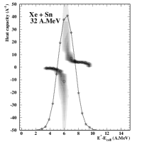
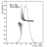
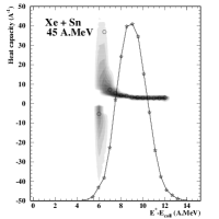
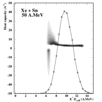
Figure 1: Microcanonical heat capacity per nucleon as a function of the thermal excitation energy (total excitation energy corrected on average for the radial collective energy).

Using a Gaussian approximation for the kinetic energy distribution its variance can be calculated as

$$A\sigma_{k}^{2}\simeq T^{2}\frac{C_{k}C_{pot}}{C_{k}+C_{pot}}.$$ (3)

Eq. (3) can be inverted to extract, from the observed fluctuations, an estimate of the microcanonical heat capacity:

$$\noindent(\frac{C}{A})_{micro}\simeq C_{k}+C_{pot}\simeq\frac{C_{k}^{2}}{C_{k}-\frac{A\sigma_{k}^{2}}{T^{2}}}.$$ (4)

From Eq. (4) we see that the specific microcanonical heat capacity $(C/A)_{micro}$ becomes negative if the normalized kinetic energy fluctuations $A\sigma_{k}^{2}/T^{2}$ overcome $C_{k}$. Figure  1 shows the results obtained [6, 7]. The heat capacity is plotted as grey zones (error bars). At 32 and 39 AMeV a negative branch is observed.

3 A detailed simulation for reconstructing freeze-out properties - the necessity to use two temperatures

Starting from the same raw data the reconstruction of freeze-out properties from simulations [20, 21] was the following. Data with a very high degree of charge completeness were selected, (measured fraction of the available charge $\geq$93% of the total charge of the system), which is crucial for a good estimate of Coulomb energy. QF sources were reconstructed, event by event, by summing the contributions of fragments (Z$\geq$5) at all angles and doubling that of light charged particles (Z$<$5) emitted between 60 and 120^∘ in the reaction centre of mass, in order to exclude the major part of pre-equilibrium emission [22, 23]; with such a prescription only light charged particles with isotropic angular distributions and angle-independent average kinetic energies are considered.

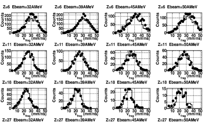
Figure 2: Comparison in the reaction centre of mass between the experimental velocity spectra of fragments of a given charge (full points) and the simulated ones (histograms). Each row refers to a different fragment charge and each column to a different beam energy. From [20].

In simulations, dressed excited fragments and particles at freeze-out are described by spheres at normal density. Then the excited fragments subsequently deexcite while flying apart. All the available asymptotic experimental information (charged particle spectra, average and standard deviation of fragment velocity spectra and calorimetry) is used to constrain the four free parameters of simulations to recover the data at each incident energy: the percentage of measured particles which were evaporated from primary fragments, the collective radial energy, a minimum distance between the surfaces of products at freeze-out and a limiting temperature for excited fragments found equal to 9 MeV. All the details of simulations can be found in refs. [20, 21]. The limiting temperature, related to the vanishing of level density for fragments [12], was found mandatory to reproduce the observed widths of fragment velocity spectra. With a single temperature (internal and kinetic temperatures equal) the sum of Coulomb repulsion, collective energy, thermal kinetic energy directed at random and spreading due to fragment decays accounts for about 60-70% of those widths. By introducing a limiting temperature, which corresponds to intrinsic temperatures for fragments in the range 4-7 MeV (see figure 1 of [24]), the thermal kinetic energy increases, due to energy conservation, thus producing the missing percentage for the widths of final velocity distributions. As shown in fig. 2, the agreement between experimental and simulated velocity spectra for fragments, for the different beam energies, is quite remarkable.

4 Direct formulae from the microcanonical ensemble - method 2

Direct formulae have been proposed in ref. [13] to calculate heat capacity but never used to extract information from data. They are derived within the microcanonical ensemble by considering fragments interacting only by Coulomb and excluded volume, which corresponds to the freeze-out configuration. Within this ensemble, the statistical weight of a configuration $c$, defined by the mass, charge and internal excitation energy of each of the constituting $M_{c}$ fragments, can be written (see [13, 25]). To apply the deduced formulae for microcanonical temperature and second derivative of the system entropy versus thermal energy or alternatively heat capacity, two parameters were fixed in the microcanonical ensemble to ensure coherence with the simulations performed to estimate quantities at freeze-out. These are the fragment level density in which the limiting temperature for fragments is fixed at 9 MeV [14] as obtained from simulations and the number of kinetic degrees of freedom which was fixed according to the conservation of energy and linear momentum as in simulations. The microcanonical temperature is deduced from its statistical definition [13]:

$$T=\left(\frac{\partial S}{\partial E^{*}}\right)^{-1} = \left(\frac{1}{\sum_{c}W_{c}}\sum_{c}W_{c}(3/2M_{c}-5/2)/K\right)^{-1}=\langle(3/2M_{c}-5/2)/K\rangle^{-1}$$ (5)

$W_{c}$ is the statistical weight of a configuration and the notation $\langle\rangle$ refers to the average over the ensemble states. The heat capacity of the system, $C$, is related to the second derivative of the entropy by the equation $\partial^{2}S/\partial E^{*2}$ = $-1/CT^{2}$. Thus, one can evaluate the second derivative of the system entropy versus $E^{*}$ (Eq. (6)) or alternatively the heat capacity $C$ (Eq. (7)).

$$\frac{\partial^{2}S}{\partial E^{*2}} = \langle\frac{(3/2M_{c}-5/2)(3/2M_{c}-7/2)}{K^{2}}\rangle-\langle\frac{(3/2M_{c}-5/2)}{K}\rangle^{2}$$ (6)

$$C=\left(1-T^{2}\langle\frac{(3/2M_{c}-5/2)(3/2M_{c}-7/2)}{K^{2}}\rangle\right)^{-1}$$ (7)

These two quantities only depend on two parameters, $M_{c}$, the total multiplicity and , $K$, the total thermal kinetic energy estimated at freeze-out from the detailed simulation.

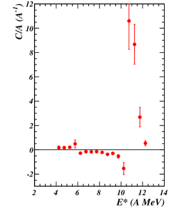
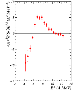
Figure 3: Heat capacity (left) and second derivative of the entropy (right) versus thermal excitation energy $E^{*}$. Error bars correspond to systematic plus statistical errors (see text). From [25].

Values of heat capacity and second derivative of the entropy versus thermal excitation energy $E^{*}$ have been calculated respectively from Eqs. (7) and (6) for QF hot nuclei with $Z$ restricted to the range 80-100 to suppress tails of the distributions and by putting together simulation results from the different incident energies. The average over the ensemble states have been assimilated to an average over “event ensembles” sorted into $E^{*}$ bins. A binning of 0.5 AMeV was chosen to have a sufficient number of events in each bin in order to reduce statistical errors. Figure 3 shows the results. Error bars correspond to systematic plus statistical errors; systematic errors were evaluated by varying the free parameters of simulations within their limits defined by a $\chi^{2}$ procedure [20]. The left part of the figure shows the results for the direct calculation of $C/A$. Negative heat capacity is observed on a rather large thermal excitation energy range and the second diverging region is more visible than the first one. As the second derivative of the entropy is a very small quantity (from $\sim 2.10^{-4}$ to $\sim 3.10^{-6}$), we have kept the presentation made in [13] i.e. $A^{2}\partial^{2}S/\partial E^{*2}$ for fig. 3 - right part; A is replaced by the average mass of the QF hot nuclei, $<A>$, on the considered $E^{*}$ bin. This quantity better defines the $E^{*}$ domain of negative heat capacity. Positive values are measured in the range 6.0 - 10.0 AMeV. The related microcanonical temperatures calculated with Eq. (5) are displayed in fig. 5; they are rather constant around 17 - 18 MeV in the $E^{*}$ range where negative heat capacity is observed. With the large multiplicities observed in the present study, microcanonical temperatures are close to classical kinetic temperatures (see figure 3 of [24]).

5 The two methods - comparison of results

As compared to heat capacity estimates of method 1 [6, 7], there is a significant difference with results of method 2 for the $E^{*}$ range of negative values: 6.0$\pm$1.0 - 10.0$\pm$1.0 AMeV for method 2 and $<$4.0$\pm$1.0 - 6.0$\pm$1.0 AMeV with method 1. For QF hot nuclei selection the same event shape sorting was used. The degree of completeness was different (93% here to be compared to 80% before) but it does not affect significantly the thermal excitation energy per nucleon.

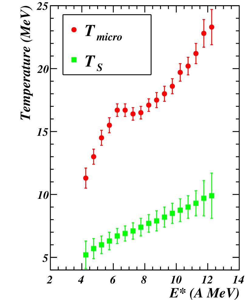
Figure 4: Evolution of temperatures with thermal excitation energy: microcanonical temperature , $T_{micro}$, used in method 2 and single temperature, $T_{S}$, for method 1. Error bars correspond to systematic plus statistical errors.

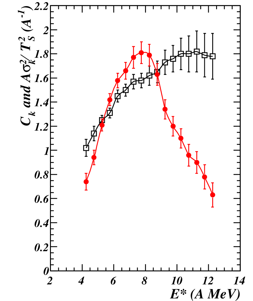
Figure 5: Normalized kinetic energy fluctuations (filled circles) and estimated $C_{k}$ values (open squares) related to method 1 (see text). Error bars correspond to systematic plus statistical errors. From [25].

The method to reconstruct freeze-out properties was also different. But the main difference seems to be related to the average freeze-out volume. In method 1 the average freeze-out volume used was kept constant at 3 times the volume at normal density (3 $V_{0}$) over the whole thermal excitation energy range whereas with the detailed simulation it varies from 3.9 to 5.9 $V_{0}$ (see fig. 4 of  [25]). To check this, method 1 has been applied to freeze-out data used with method 2. From the detailed simulation, for each $E^{*}$ bin, we have calculated $<E_{k}>$ (see Eq. (1)) and derived an apparent single temperature, $T_{S}$ (see fig. 5), needed to build the normalized kinetic energy fluctuations, $A\sigma_{k}^{2}$/$T_{S}^{2}$, to be compared to $C_{k}$ (see Eqs. (2) and (4)). Figure 5 shows that heat capacity becomes negative in the $E^{*}$ range 5.5$\pm$1.0 - 9.0$\pm$1.0 AMeV, i.e. when $A\sigma_{k}^{2}$/$T_{S}^{2}$ overcomes $C_{k}$. This clearly confirms that the main difference, as compared to estimates with method 1, comes from different average freeze-out volumes. We also note a small decrease of the $E^{*}$ domain of negative heat capacities as compared to method 2, which possibly comes from approximations made in method 1.

6 Conclusion

Heat capacity measurements have been revisited without approximation and by correcting the hypothesis of a single temperature associated with both internal excitation and thermal motion of fragments. For those measurements microcanonical formulae and data reconstructed at freeze-out with the help of a detailed simulation have been used. Negative heat capacity was confirmed for hot nuclei in the coexistence region of the liquid-gas phase transition. For the future, one of the last points to be also deeper investigated is the bimodality signature for QF hot nuclei. As demonstrated for $\Delta$-scaling, the effect of the onset and increase of radial expansion must be understood [3, 26, 27, 22].

References

- [1] CHOMAZ P.et al. (eds.), Eur. Phys. J. A 30 (2006) and references therein.
- [2] BORDERIE B. and RIVET M.F., Prog. Part. Nucl. Phys. 61 (2008) 551.
- [3] BORDERIE B. and FRANKLAND J.D., Prog. Part. Nucl. Phys. 105 (2019) 82.
- [4] CHOMAZ P. et al., Phys. Rep. 389 (2004) 263.
- [5] D’AGOSTINO M. et al., Phys. Lett. B 473 (2000) 219.
- [6] LE NEINDRE N. et al. in Proceedings of the XXXVIII International Winter Meeting on Nuclear Physics, Bormio, Italy, edited by I. Iori and A. Moroni, suppl. 116 (Ricerca Scientifica ed Educazione Permanente (2000) p. 404.
- [7] BORDERIE B., J. Phys. G: Nucl. Part. Phys. 28 (2002) R217.
- [8] CHOMAZ P. and GULMINELLI F., Nucl. Phys. A 647 (1999) 153.
- [9] CHOMAZ P. et al., Phys. Rev. Lett. 85 (2000) 3587.
- [10] TUBBS D.L. and KOONIN S.E., Ap. J. 232 (1979) L59.
- [11] DEAN D.R. and MOSEL U., Z. Phys. A 322 (1985) 647.
- [12] KOONIN S.E., and RANDRUP J., Nucl. Phys. A 474 (1987) 173.
- [13] RADUTA Al. H. and RADUTA Ad. R., Nucl. Phys. A 703 (2002) 876.
- [14] RADUTA Al. H. and RADUTA Ad. R., Phys. Rev. C 61 (2000) 034611.
- [15] POUTHAS J. et al., Nucl. Instr. and Meth. in Phys. Res. A 357 (1995) 418.
- [16] POUTHAS J. et al., Nucl. Instr. and Meth. in Phys. Res. A 369 (1996) 222.
- [17] TĂBĂCARU G. et al., Nucl. Instr. and Meth. in Phys. Res. A 428 (1999) 379.
- [18] PÂRLOG M. et al., Nucl. Instr. and Meth. in Phys. Res. A 482 (2002) 693.
- [19] D’AGOSTINO M. et al., Nucl. Phys. A 699 (2002) 795.
- [20] PIANTELLI S. et al., Nucl. Phys. A 809 (2008) 111.
- [21] PIANTELLI S. et al., Phys. Lett. B 627 (2005) 18.
- [22] BONNET E. et al., Nucl. Phys. A 816 (2009) 1.
- [23] FRANKLAND J. D. et al., Nucl. Phys. A 689 (2001) 940.
- [24] BORDERIE B. et al., Phys. Lett. B 723 (2013) 140.
- [25] BORDERIE B. et al., Eur. Phys. J. A 56 (2020) 101.
- [26] FRANKLAND J. D. et al., Phys. Rev. C 71 (2005) 034607.
- [27] GRUYER D. et al., Phys. Rev. Lett. 110 (2013) 172701.