Prospects for constraining interacting dark energy models from gravitational wave and gamma ray burst joint observation

Abstract

With the measurement of the electromagnetic (EM) counterpart, a gravitational wave (GW) event could be treated as a standard siren. As a novel cosmological probe, GW standard sirens will bring significant implications for cosmology. In this paper, by considering the coincident detections of GW and associated $\gamma$ ray burst (GRB), we find that only about 400 GW bright standard sirens from binary neutron star mergers could be detected in a 10-year observation of the Einstein Telescope and the THESEUS satellite mission. Based on this mock sample, we investigate the implications of GW standard sirens on the interaction between dark energy and dark matter. In our analysis, four viable interacting dark energy (IDE) models, with interaction forms $Q=3\beta H\rho_{\mathrm{de}}$ and $Q=3\beta H\rho_{\mathrm{c}}$, are considered. Compared with the traditional EM observational data such as CMB, BAO, and SN Ia, the combination of both GW and EM observations could effectively break the degeneracies between different cosmological parameters and provide more stringent cosmological fits. We find that the GW data could play a more important role for determining the interaction in the models with $Q=3\beta H\rho_{\mathrm{c}}$, compared with the models with $Q=3\beta H\rho_{\mathrm{de}}$. We also show that constraining IDE models with mock GW data based on different fiducial $H_{0}$ values yield different results, indicating that accurate determination of $H_{0}$ is significant for exploring the interaction between dark energy and dark matter.

1 Introduction

The last few decades of cosmological study lead us to a standard cosmological scenario, the so-called $\Lambda$ cold dark matter model ($\Lambda$CDM) with six free parameters, which is in remarkable agreement with the bulk of cosmological observations [1, 2, 3, 4, 5, 6, 7]. This model is featured by dark components including dark matter and dark energy, and dark energy in this model is provided by a cosmological constant $\Lambda$. However, the validity of $\Lambda$CDM has been threatened in recent years on both theoretical and observational grounds. In theory, the cosmological constant $\Lambda$ always suffers from several severe puzzles, such as the “fine-tuning” and “cosmic coincidence” problems [8, 9, 10]. In observation, the measurement inconsistencies of some key cosmological parameters, the Hubble constant $H_{0}$ and cosmic curvature parameter $\Omega_{k}$ for example, are posing a serious challenge to the standard cosmological model [6, 11, 7, 12, 13, 14, 15, 16, 17, 18, 19, 20]. Therefore, some important cosmological issues need to be reexamined in the context of the serious crisis for the standard cosmology. In fact, all of these problems are relevant to the fundamental natures of dark energy and dark matter. For example, dynamical dark energy with the equation of state (EoS) $w<-1$ can help relieve the $H_{0}$ tension. The interacting dark energy (IDE) model considering a coupling between dark energy and dark matter not only can alleviate the Hubble tension [14, 21, 22, 23, 24, 25], but also can alleviate the “fine-tuning” and “cosmic coincidence” problems through the attractor solution [26, 27, 28, 29, 30]. Additionally, the coupling between dark energy and dark matter is an important theoretical possibility whose confirmation or denial would have enormous implications for fundamental physics. Although the existing observational constraints indicate that the coupling between dark energy and dark matter is weak, they still cannot be ruled out by observations [31, 32, 33, 34, 25, 35, 36, 37, 38, 39, 14, 21, 22, 23, 24]. Therefore, it is rewarding to test the IDE models by using other complementary cosmological probes including the gravitational wave (GW) observation (especially the inspiraling and merging compact binaries).

The discovery of GW event GW150914 as the first directly detected GW signal marked the arrival of the era of GW astronomy [40, 41]. In particular, the later GW170817 event from a binary neutron star (BNS) merger and the successful detections of associate electromagnetic (EM) waves in various bands brought us to a new era of multi-messenger astronomy [42, 43]. The measurement of GW signal could directly provide the luminosity distance to the source without any additional calibration, and its redshift can be determined by detecting its remaining kilonova emission in the EM band (in the case of BNS), which enables us to establish the luminosity distance-redshift relation [44, 45, 46]. This is called the standard siren method, which is extremely important for studying cosmology, especially for exploring the constituents of the universe [47, 48, 49, 50, 51, 52, 53, 54, 55, 56, 57, 58, 59, 60, 61, 62]. However, until now, the only GW bright standard siren event available in cosmology still remains the GW170817. Compared with the current ground-based GW detector network LIGO-Virgo-KAGRA, the upcoming Einstein Telescope (ET) as a third-generation ground-based GW observatory with 10 km-long arms and three detectors has a much wider detection frequency range and a much better detection sensitivity [63]. It is expected to detect abundant standard sirens from the BNS mergers in a 10-year observation [47, 64].

In this paper, we aim to investigate the impacts of the future GW standard siren observations on the constraint of the coupling between dark energy and dark matter. Although some authors have discussed these related issues [65, 60, 66], we highlight some improvements in this paper as follows.

In previous studies on constraints on cosmology with future GW observations [65], the simulated process of GW standard sirens was too rough. It was common to assume that ET could detect 1000 GW standard sirens, which is only a rough estimation. However, determining the redshift for a GW standard siren requires the observation of the EM counterpart. One effective method is to detect a temporally coincident $\gamma$-ray burst (GRB) that can be precisely localized. In this paper, we consider the possibility of simultaneous detection of a joint GW-GRB event. Based on the latest studies about joint GW-GRB observations, we construct a mock catalog of standard sirens from ET by considering the coincidences with a GRB detector. This makes it more reasonable to realistically predict the constraints on the IDE models by the future GW standard siren data.

In the simulated process of GW, the previous studies [65, 60, 66] adopted the $\Lambda$CDM model with the parameters taken from the Planck 2018 results [7], $\Omega_{m}=0.315$ and $H_{0}=67.4~{}\mathrm{km~{}s^{-1}~{}Mpc^{-1}}$, as the fiducial cosmology. However, the late-universe observations, the local type Ia supernovae (SN Ia) data calibrated by the distance ladder, reported a high value of the Hubble constant $H_{0}=73.2\pm 1.3~{}\mathrm{km~{}s^{-1}~{}Mpc^{-1}}$ [67], which is in tension with the Planck data. As an independent probe of the late universe, GW data are more likely to infer a $H_{0}$ value matched with the one inferred by SN Ia data. Therefore, to discuss how robust the constraints on the IDE models from GWs are when the fiducial cosmology is altered, we will simulate the GW data based on two different fiducial $H_{0}$ values, respectively, and discuss their constraints on the IDE models.

In the previous papers [65, 60, 66], the interaction terms between dark energy and dark matter are considered proportional to the density of cold dark matter. However, the physical mechanism of the interaction is unclear at present. More discussions of the possibilities would be helpful. In this paper, we will not only consider the interaction terms proportional to the density of cold dark matter but also the interaction terms proportional to the density of dark energy.

Previous studies showed that GW standard sirens, as absolute-distance measurements, are fairly good at constraining the Hubble constant [68] but not good at constraining other cosmological parameters [59, 47, 48, 45, 50, 51, 52, 53, 60, 61, 56, 57, 58, 46, 69, 70]. However, it is found that GW standard sirens are highly complementary with some conventional cosmological probes, including the cosmic microwave background (CMB), baryon acoustic oscillations (BAO), and SN Ia in constraining dark energy models. Such data combinations could effectively break the parameter degeneracies and give tighter constraints on cosmological parameters. Therefore, in this paper, we also employ the mainstream cosmological probes combined with the simulated GW standard siren data from ET to thoroughly investigate the GW’s role in studying the IDE models. The traditional observational data sets used in this paper include CMB, BAO, and SN Ia. Compared to the previous works, we will employ the latest SN Ia “Pantheon+” compilation [71], containing 1701 light curves of 1550 unique objects, instead of the “Pantheon” data containing 1048 data points. There are many improvements, including the sample size, the treatments of systematic uncertainties in redshift, peculiar velocities, photometric calibration, and intrinsic scatter model of SN Ia, which greatly enhance the constraining capability of the Pantheon+ compilation compared with the original Pantheon compilation [71]. Therefore, our work in this paper includes the latest constraints on the IDE model from traditional observational data. For the CMB measurements, we use the Planck distance priors $\left(R,\ell_{A},\Omega_{b}h^{2}\right)$ obtained from the Planck 2018 TT,TE,EE+lowE data [7, 72]. For the BAO data, we consider several measurements from 6dFGS [73], SDSSMGS [74], and BOSS DR12 [75].

2 Interacting dark energy models

In a flat universe described by the Friedmann-Lemaître-Robertson-Walker metric, the dimensionless Hubble parameter $E(z)=H(z)/H_{0}$ could be written as

$$E^{2}=\Omega_{\mathrm{de}0}\frac{\rho_{\mathrm{de}}}{\rho_{\mathrm{de}0}}+\Omega_{\mathrm{c}0}\frac{\rho_{\mathrm{c}}}{\rho_{\mathrm{c}0}}+\Omega_{\mathrm{b}0}\frac{\rho_{\mathrm{b}}}{\rho_{\mathrm{b}0}}+\Omega_{\mathrm{r}0}\frac{\rho_{\mathrm{r}}}{\rho_{\mathrm{r}0}},$$ (2.1)

where $\Omega_{\mathrm{de}0}$, $\Omega_{\mathrm{c}0}$, $\Omega_{\mathrm{b}0}$ and $\Omega_{\mathrm{r}0}$ are current energy density fractions of dark energy, cold dark matter (CDM), baryon and radiation, respectively. Here, we have $\rho_{\mathrm{b}}=\rho_{\mathrm{b}0}(1+z)^{3}$ and $\rho_{\mathrm{r}}=\rho_{\mathrm{r}0}(1+z)^{4}$, where $z$ denotes the redshift. Considering the interaction between dark energy and CDM, we have the energy continuity equations

$$(1+z)\frac{\mathrm{d}\rho_{\mathrm{de}}}{\mathrm{d}z}-3(1+w)\rho_{\mathrm{de}}=\frac{Q}{H},$$ (2.2)

$$(1+z)\frac{\mathrm{d}\rho_{\mathrm{c}}}{\mathrm{d}z}-3\rho_{\mathrm{c}}=-\frac{Q}{H},$$

where $Q$ denotes a phenomenological interaction term, and $w$ is the EoS of dark energy. The form of $Q$ is an open question. However, it is usually assumed to be proportional to the density of dark sectors. In this paper, we consider two forms of the interaction term, i.e., $Q_{1}=3\beta H\rho_{\mathrm{de}}$ and $Q_{2}=3\beta H\rho_{\mathrm{c}}$, where $\beta$ is a dimensionless coupling parameter describing the strength of the interaction between dark energy and dark matter. $\beta>0$ means that dark matter will be converted into dark energy, and vice versa for $\beta<0$. If $\beta=0$, it indicates no interaction between the two sectors.

For the EoS of dark energy $w$, we consider two cases, i.e., the case of $w=-1$, denoted as I$\Lambda$CDM, and the case of $w$ being a constant, denoted as I$w$CDM. Thus, we will have four IDE models, I$\Lambda$CDM1, I$\Lambda$CDM2, I$w$CDM1, and I$w$CDM2. For the I$w$CDM1 model (with $Q_{1}=3\beta H\rho_{\mathrm{de}}$), the dimensionless Hubble parameter satisfies [76, 37, 77]

$$E^{2}(z)= \Omega_{\mathrm{de}0}\left(\frac{\beta}{w+\beta}(1+z)^{3}+\frac{w}{w+\beta}(1+z)^{3(1+w+\beta)}\right)$$ (2.3)

$$+\Omega_{\mathrm{m}0}(1+z)^{3}+\Omega_{\mathrm{r}0}(1+z)^{4}.$$

For the I$w$CDM2 model (with $Q_{2}=3\beta H\rho_{\mathrm{c}}$), we have [76, 37, 77]

$$E^{2}(z)= \Omega_{\mathrm{de}0}(1+z)^{3(1+w)}+\Omega_{\mathrm{b}0}(1+z)^{3}+\Omega_{\mathrm{r}0}(1+z)^{4}$$ (2.4)

$$+\Omega_{\mathrm{c}0}\left(\frac{\beta}{w+\beta}(1+z)^{3(1+w)}+\frac{w}{w+\beta}(1+z)^{3(1-\beta)}\right).$$

Setting $w=-1$ in the above two expressions, the corresponding expressions for I$\Lambda$CDM1 and I$\Lambda$CDM2 could be obtained.

3 Gravitational wave simulation

In this paper, we wish to realistically forecast the constraints on the IDE models from GW standard sirens detected by ET. To construct a mock catalogue of standard sirens, not only the detectable mergers of BNS should be considered, but also more importantly, whether the associated EM counterparts are able to be detected should be considered. Therefore, in this work, we consider Transient High-Energy Sky and Early Universe Surveyor (THESEUS) mission [78, 79, 80], a space telescope proposed to study GRB and X-rays, to predict the associated GRBs with GWs.

Based on the star formation rate [81, 82, 83], the merger rate of BNS density per unit redshift is

$$R_{z}(z)=\frac{R_{m}(z)}{(1+z)}\frac{dV(z)}{dz},$$ (3.1)

where $dV/dz$ is the comoving volume element. $R_{m}(z)$ represents the rate per volume in the source frame, which is related to the time delay between the formation of the BNS progenitors and their mergers as

$$R_{m}(z)=\int_{z}^{\infty}\frac{dt_{f}}{dz_{f}}R_{f}(z_{f})P(t_{d})dz_{f},$$ (3.2)

where $R_{f}$ is the formation rate of massive binaries and $P(t_{d})$ is the distribution of the time delay $t_{d}$. A BNS system that merges at the look-back time $t$ is formed at the look-back time $t_{f}$, and the time delay $t_{d}$ is $t_{f}-t$. Here, the formation rate of massive binaries $R_{f}$ is assumed to be proportional to the cosmic star formation rate, for which we adopt the Madau-Dickinson model [84],

$$\psi_{\rm{MD}}=\psi_{0}\frac{(1+z)^{\alpha^{\prime}}}{1+[(1+z)/C]^{\beta^{\prime}}},$$ (3.3)

with parameters $\alpha^{\prime}=2.7$, $\beta^{\prime}=5.6$, $C=2.9$ and $\psi_{0}=0.015~{}\rm{M_{\odot}~{}Mpc^{-3}yr^{-1}}$. The proportionality coefficient is the normalization factor that ensures today the merger rate is $R_{m}(z=0)=R_{0}$, for which we use $R_{0}=920~{}\rm{Gpc^{-3}yr^{-1}}$ estimated from the O1 LIGO and O2 Ligo/Virgo observation run [85]. For the time delay distribution $P(t_{d})$, we follow and adopt the exponential form [81],

$$P(t_{d})=\frac{1}{\tau}\exp(-t_{d}/\tau),$$ (3.4)

with time scale parameter $\tau=0.1~{}\rm{Gyr}$. Thus, we can obtain the BNS merger rate density per unit redshift.

To obtain the detectable number and distribution of GW events, we need to calculate the signal-to-noise ratio (SNR) for each GW event and select the event whose SNR is larger than the sensitivity threshold of the GW detector. For the calculation of the SNR for a GW event, we refer to the detailed description in Refs. [47, 64], and we do not repeat it here. For the threshold of ET, we take it to be $\rho_{\rm{threshold}}=8$. We assume a running period of 10 years and a duty cycle of 80%. In the left panel of figure 1, we show the redshift distribution of GW events from a realization of the mock catalogue for the ET in a 10-year observation.

For the BNSs used as standard sirens, the redshift information of sources is necessary, which could usually be inferred by the observations of electromagnetic counterparts. To estimate the number and distribution of coincidences between GW events and EM counterparts, the available network of GRB satellites and telescopes when the GW detector is triggered is very crucial. In the following, we combine the THESEUS mission to calculate the detection rate of GW-GRB standard sirens.

For a GRB detected in coincidence with a GW signal, the peak flux should be larger than the flux limit of the satellite. Based on the analysis of GRB170817A [86], we adopt the Gaussian structured jet profile model,

$$L\left(\theta_{\mathrm{V}}\right)=L_{\mathrm{c}}\exp\left(-\frac{\theta_{\mathrm{V}}^{2}}{2\theta_{\mathrm{c}}^{2}}\right),$$ (3.5)

where $L\left(\theta_{\mathrm{V}}\right)$ is the luminosity per unit solid angle, $\theta_{\mathrm{V}}$ is the viewing angle, $L_{\mathrm{c}}$ and $\theta_{\mathrm{c}}$ are structure parameters defined the angular profile. The structured jet parameter is given by $\theta_{\mathrm{c}}=4.7^{\circ}$. $L_{\mathrm{c}}=L_{\mathrm{p}}/4\pi$ erg s^-1 sr^-1, where $L_{\rm{p}}$ is the peak luminosity of each burst. Next, to determine if a GRB could be detected, we need to convert the flux threshold of the GRB satellite $P_{\rm{T}}$ to the luminosity, which could be implemented by

$$L=4\pi d_{L}^{2}(z)k(z)b/(1+z)P_{T}.$$ (3.6)

$b$ is an energy normalization to account for the missing fraction of the $\gamma$-ray energy seen in the detector band [87, 86], and its expression is

$$b=\frac{\int_{10000}^{1}EN(E)dE}{\int_{E1}^{E2}N(E)dE},$$ (3.7)

where $N(E)$ is the observed GRB photon spectrum in units of $\rm{ph~{}s^{-1}~{}keV^{-1}~{}cm^{-2}}$, and $[E1,E2]$ is the detector’s energy window. $k(z)$ represents a k-correction [87, 86],

$$k(z)=\frac{\int_{E1}^{E2}N(E)dE}{\int_{E1(1+z)}^{E2(1+z)}N(E)dE}.$$ (3.8)

For the observed GRB photon spectrum, we model it by the Band function, which is a function of spectral indices ($\alpha_{B}$, $\beta_{B}$) and break energy $E_{b}$, expressed as [88]

$$N(E)=\begin{cases}N_{0}\left(\frac{E}{100\mathrm{keV}}\right)^{\alpha_{B}}\exp\left(-\frac{E}{E_{0}}\right),&E\leq E_{b}\\ N_{0}\left(\frac{E_{b}}{100\mathrm{keV}}\right)^{\alpha_{B}-\beta_{B}}\exp\left(\beta_{B}-\alpha_{B}\right)\left(\frac{E}{100\mathrm{keV}}\right)^{\beta_{B}},&E>E_{b}\end{cases},$$ (3.9)

where $E_{b}=\left(\alpha_{B}-\beta_{B}\right)E_{0}$ and $E_{p}=\left(\alpha_{B}+2\right)E_{0}$. We take $\alpha_{B}=-0.5$, $\beta_{B}=-2.25$ and a peak energy $E_{p}=800~{}\rm{keV}$.

For the distribution of the short GRBs, we assume a standard broken power law model,

$$\Phi\left(L\right)\propto\begin{cases}\left(L/L_{*}\right)^{\alpha_{L}},&L<L_{*}\\ \left(L/L_{*}\right)^{\beta_{L}},&L\geq L_{*}\end{cases},$$ (3.10)

with the characteristic parameter separating the two regimes $L_{*}=2\times 10^{52}~{}\rm{erg~{}sec^{-1}}$, and two slopes parameters $\alpha_{L}=-1.95$ and $\beta_{L}=-3$ [87]. For the THESEUS mission [79], it is recorded if the value of the observed flux is larger than the flux threshold $P_{\rm{T}}=0.2~{}\rm{ph~{}sec^{-1}~{}cm^{-2}}$ in the $50-300$ keV band. According to the THESEUS paper [79], we take a sky coverage fraction of 0.5 and a duty cycle of 80%. Then we can calculate the probability of the GRB detection for every GW event according to the probability distribution $\Phi(L)dL$. Finally, we find that only about 400 standard sirens could be detected for the ET+THESEUS network in 10 years, whose redshift distribution is shown in the right panel of figure 1.

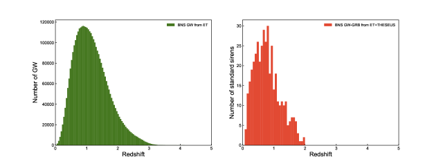
Figure 1: The redshift distribution of the mock catalogue for a 10-year detection of BNS GW (left) from ET and GW-GRB standard sirens (right) from ET+THESEUS.

In order to discuss the influence of GW simulation based on different fiducial $H_{0}$ values on the final results, two sets of GW data will be simulated here. We adopt two fiducial cosmological models, both of which are the $\Lambda$CDM models, but with different parameter values. One model uses the parameter values from Planck 2018 results [7], namely $\Omega_{\rm{m}}=0.315$ and $H_{0}=67.4~{}\mathrm{km~{}s^{-1}~{}Mpc^{-1}}$, while the other model use $\Omega_{\rm{m}}=0.315$ from Planck 2018, but $H_{0}=73.2~{}\mathrm{km~{}s^{-1}~{}Mpc^{-1}}$ from SH0ES Collaboration [67]. According to the error strategy, we consider the instrumental error $\sigma_{D_{L}}^{\text{inst }}$ and an additional error $\sigma_{D_{L}}^{\text{lens }}$ caused by the weak lensing to the total uncertainty of the luminosity distance as

$$\sigma_{D_{L}}=\sqrt{\left(\sigma_{D_{L}}^{\text{inst }}\right)^{2}+\left(\sigma_{D_{L}}^{\text{lens }}\right)^{2}}.$$ (3.11)

The instrumental error of the luminosity distance is dependent on the signal-to-noise ratio (SNR) $\rho$ of a GW signal as $\sigma_{D_{L}}^{\text{inst}}\simeq D_{L}/\rho$ [47]. For the ET, to confirm a detected GW signal is using the criteria that the combined SNR is larger than 8 [47, 64]. To consider the correlation between the inclination angle $\iota$ and the luminosity distance, we add a factor 2 in front of the error [64], $\sigma_{D_{L}}^{\text{inst}}\simeq 2D_{L}/\rho$. The lensing uncertainty is modelled as $\sigma_{D_{L}}^{\text{lens }}=0.05zD_{L}$ [64].

4 Results and discussions

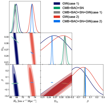
Figure 2: The constraints (68.3% and 95.4% confidence level) on the I$\Lambda$CDM1 model with $Q=3\beta H\rho_{\rm{de}}$ from GW, CMB+BAO+SN, and CMB+BAO+SN+GW. Case 1 denotes the simulated GW data with $H_{0}=67.4~{}\mathrm{km~{}s^{-1}~{}Mpc^{-1}}$, and case 2 represents the one with $H_{0}=73.2~{}\mathrm{km~{}s^{-1}~{}Mpc^{-1}}$, respectively.

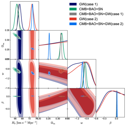
Figure 3: Same as figure 2 but for the I$w$CDM1 model with $Q=3\beta H\rho_{\rm{de}}$.

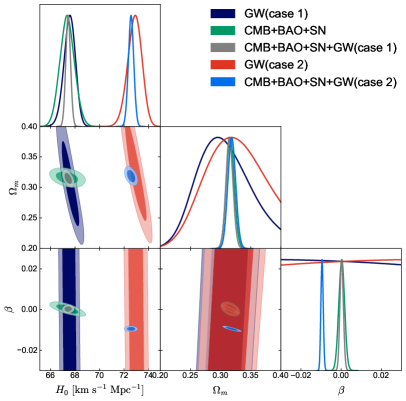
Figure 4: Same as figure 2 but for the I$\Lambda$CDM2 model with $Q=3\beta H\rho_{\rm{c}}$.

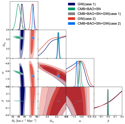
Figure 5: Same as figure 2 but for the I$w$CDM2 model with $Q=3\beta H\rho_{\rm{c}}$.

Model	Parameter	CMB+BAO+SN	GW(case 1)	CMB+BAO+SN+GW(case 1)	GW(case 2)	CMB+BAO+SN+GW(case 2)
I$\Lambda$CDM1 ($Q_{1}=3\beta H\rho_{\rm{de}}$)	$H_{0}$	$67.44\pm{0.50}$	$67.90^{+0.56}_{-0.62}$	$67.45\pm{0.20}$	$73.15^{+0.63}_{-0.72}$	$73.01\pm{0.22}$
	$\Omega_{\rm m}$	$0.3164\pm{0.0066}$	$0.251^{+0.088}_{-0.071}$	$0.3163\pm{0.0029}$	$0.290^{+0.093}_{-0.072}$	$0.2546\pm{0.0023}$
	$\beta$	$0.0003\pm{0.0036}$	$-0.15^{+0.21}_{-0.18}$	$-0.0003\pm{0.0032}$	$-0.06^{+0.22}_{-0.18}$	$0.0152\pm{0.0022}$
I$w$CDM1 ($Q_{1}=3\beta H\rho_{\rm{de}}$)	$H_{0}$	$66.66\pm{0.70}$	$67.90\pm 0.60$	$67.25\pm{0.28}$	$72.92\pm 0.70$	$73.32\pm{0.30}$
	$\Omega_{\rm m}$	$0.3203\pm 0.0071$	$>0.266$	$0.3157\pm{0.0029}$	$0.37^{+0.19}_{-0.12}$	$0.2546\pm{0.0023}$
	$w$	$-0.944\pm 0.036$	$-1.23^{+0.43}_{-0.28}$	$-0.972\pm{0.029}$	$-1.14^{+0.45}_{-0.22}$	$-1.030\pm{0.023}$
	$\beta$	$0.0012\pm 0.0045$	$0.08^{+0.30}_{-0.39}$	$0.0008^{+0.0045}_{-0.0041}$	$0.11^{+0.39}_{-0.23}$	$0.0131\pm 0.0029$
I$\Lambda$CDM2 ($Q_{2}=3\beta H\rho_{\rm{c}}$)	$H_{0}$	$67.37\pm 0.60$	$67.55^{+0.50}_{-0.43}$	$67.44\pm{0.19}$	$72.87^{+0.61}_{-0.54}$	$72.57\pm{0.22}$
	$\Omega_{\rm m}$	$0.3160\pm 0.0065$	$0.312^{+0.035}_{-0.057}$	$0.3148\pm{0.0059}$	$0.335^{+0.044}_{-0.068}$	$0.3186\pm{0.0065}$
	$\beta$	$0.0003\pm 0.0015$	$0.01^{+0.24}_{-0.32}$	$0.0003\pm{0.0009}$	$0.08^{+0.24}_{-0.30}$	$0.0095\pm{0.0006}$
I$w$CDM2 ($Q_{2}=3\beta H\rho_{\rm{c}}$)	$H_{0}$	$65.9\pm{1.1}$	$67.74\pm{0.62}$	$67.34\pm{0.27}$	$72.96\pm{0.72}$	$73.41\pm{0.31}$
	$\Omega_{\rm m}$	$0.3202\pm{0.0071}$	$0.388^{+0.18}_{-0.091}$	$0.3148\pm{0.0060}$	$>0.291$	$0.3146\pm{0.0064}$
	$w$	$-0.946\pm{0.035}$	$-1.26^{+0.47}_{-0.28}$	$-0.988\pm{0.021}$	$-1.16^{+0.47}_{-0.28}$	$-1.086\pm{0.023}$
	$\beta$	$0.0020\pm{0.0019}$	$0.12^{+0.36}_{-0.20}$	$0.0002\pm{0.0009}$	$>0.0414$	$-0.0089\pm{0.0006}$

Table 1: The constraints on cosmological parameters of the I$\Lambda$CDM1, I$w$CDM1, I$\Lambda$CDM2 and I$w$CDM2 models from GW, CMB+BAO+SN and CMB+BAO+SN+GW. Case 1 denotes the simulated GW data with $H_{0}=67.4~{}\mathrm{km~{}s^{-1}~{}Mpc^{-1}}$, and case 2 represents the one with $H_{0}=73.2~{}\mathrm{km~{}s^{-1}~{}Mpc^{-1}}$, respectively. Here $H_{0}$ is in units of $\rm km\ s^{-1}\ Mpc^{-1}$.

The main results are shown in figures 2–5 and table 1. Figure 2 shows the constraints on the I$\Lambda$CDM1 model with $Q=3\beta H\rho_{\rm{de}}$ from GW, CMB+BAO+SN and CMB+BAO+SN+GW. It is important to emphasize that the central values of the cosmological parameters obtained from the simulated GW data are not meaningful in themselves, and only the errors are relevant. However, we find that the two simulated GW data sets with two different fiducial $H_{0}$ values yield different results for the constraint uncertainties on the IDE models. This shows that the central values of parameters can actually make some impacts on the constraint errors, and thus they are somewhat meaningful in this sense. Therefore, we still list the best-fit values from the simulated data in table 1, but it is important to keep in mind that only the constraint errors are meaningful for a forecast study.

Here, we denote the results from the simulated GW data with the fiducial $H_{0}=67.4~{}\mathrm{km~{}s^{-1}~{}Mpc^{-1}}$ as case 1 and denote the one with the fiducial $H_{0}=73.2~{}\mathrm{km~{}s^{-1}~{}Mpc^{-1}}$ as case 2. In both cases, we can see that the constraint on $H_{0}$ with GW data alone is tight and comparable with that from CMB+BAO+SN because GWs provide the measurements of absolute distances with high sensitivity to $H_{0}$. For $\Omega_{\rm{m}}$ and $\beta$, GW alone gives a weaker constraint than CMB+BAO+SN. However, the parameters degeneracy directions from GW and CMB+BAO+SN are rather different, especially in the $H_{0}-\Omega_{\rm{m}}$ and $H_{0}-\beta$ planes. Therefore, their combination could effectively break the degeneracies between parameters and give tight constraints on all parameters. With respect to the $\beta$ describing the strength of the interaction between dark energy and dark matter, we find that the data sets CMB+BAO+SN can give a tight constraint on it, $\beta=0.0003\pm{0.0036}$, which suggests that there is no interaction between dark energy and dark matter. Since the interaction term is proportional to $H(z)$, the CMB measurements in the early universe have a relatively strong ability to constrain the dimensionless coupling parameter $\beta$. Conversely, the GW measurements of the late universe have a weak constraint ability to it as shown in figure 2. However, GW combined with CMB+BAO+SN is still beneficial in breaking the degeneracy between $\beta$ and other parameters.

Comparing the two cases, we find that the constraints on $H_{0}$ are very different, whether using GW data alone or combined with CMB+BAO+SN, which indicates that GW data play a dominant role in constraining $H_{0}$. Moreover, since the degeneracy directions of GW and CMB+BAO+SN are quite different, the best-fit values of parameters from the combined CMB+BAO+SN with two GW cases, respectively, should be affected. For example, CMB+BAO+SN+GW (case 1) gives a result of $\Omega_{\rm{m}}=0.3163\pm 0.0029$, while a shifted best-fit value of $\Omega_{\rm{m}}=0.2546\pm 0.0023$ is obtained by the data set of CMB+BAO+SN+GW (case 2). In particular, the constraints on the interaction parameter $\beta$ are also greatly affected. The CMB+BAO+SN+GW (case 1) data give a result of $\beta=-0.0003\pm 0.0032$ in excellent agreement with the zero interaction, while the result of $\beta=-0.0152\pm 0.0022$ from the CMB+BAO+SN+GW (case 2) data supports that there is an interaction between dark energy and dark matter. Therefore, we conclude that an accurate measurement of $H_{0}$ is very helpful to explore the interaction between dark energy and dark matter.

For the I$w$CDM1 model, we find that CMB+BAO+SN can offer tight constraints on all parameters, while GW data only give weak constraints on all parameters except $H_{0}$. However, all parameters can be constrained more stringent with the help of combining with GW data. For instance, the constraint precision of $H_{0}$ and $\Omega_{\rm{m}}$ is improved by a factor of two when the CMB+BAO+SN data combine with GW. Concerning the coupling constant $\beta$, a tight constraint from existing CMB+BAO+SN, $\beta=0.0012\pm{0.0045}$, also indicates that there is no interaction between two dark sectors. When combined with GW (case 1), we find that the constraint on the interaction parameter $\beta$ is not significantly improved, with a result of $\beta=0.0008^{+0.0045}_{-0.0041}$. However, when combined with GW (case 2), the error of $\beta$ improves to $0.0029$, but its best-fit value shifts to 0.0131, which means dark matter decay into dark energy.

The results of I$\Lambda$CDM2 model with $Q=3\beta H\rho_{\rm{c}}$ are shown in figure 4 and table 1. Similar to the case of the I$\Lambda$CDM1 model, GW data alone give weak constraints on all parameters except $H_{0}$, while all parameters can be constrained very well by the CMB+BAO+SN data. The CMB+BAO+SN data combined with GW could significantly break the degeneracies between parameters and give tighter constraints on all parameters. For the coupling parameter $\beta$, we obtain $\beta=0.0003\pm{0.0015}$ from the CMB+BAO+SN and $\beta=0.0003\pm{0.0009}$ from CMB+BAO+SN+GW (case 1). With the addition of the GW data (no matter case 1 or case 2), the constraint precision of $\beta$ is improved by a factor of two. In this paper, we improve the simulation of GW to make it more reasonable and realistic. We note that our results are very close but slightly different from the previous results for the same IDE model. With respect to the coupling parameter $\beta$, Li et al. [65] obtained $\beta=0.00120\pm{0.00088}$ from the CMB+BAO+SN+GW data, in which the GW data are simulated with the fiducial $H_{0}=67.4~{}\mathrm{km~{}s^{-1}~{}Mpc^{-1}}$. It should be noted that the form of the interaction term they adopt is $Q=\beta H\rho_{\rm{c}}$, a factor of 3 different from the one we used. Therefore, the precision of their constraint on $\beta$ translated into our form should be 0.00029, a little better than that we obtained. The reason for this is that the number of GW standard sirens we obtained is only 400 by taking into account the coincident GRB detection, while Li et al. [65] just roughly assume 1000 GW standard sirens. In addition, for case 2, the CMB+BAO+SN+GW (case 2) data give a result of $\beta=0.0095\pm 0.0006$, which is deviated from zero.

Finally, we investigate the I$w$CDM2 model with $Q=3\beta H\rho_{\rm{c}}$, of which the results are shown in figure 5 and table 1. As the number of parameters increases, we find that GW alone has a weak ability to constrain parameters. However, its parameter degeneracy direction is rather different from that of the CMB+BAO+SN data. Therefore, the combination of them could significantly improve the constraint of parameters. Compared with the constraint value of $\beta$ in the previous work [65], $\beta=-0.0005\pm 0.0004$ from CMB+BAO+SN+GW, the error of $0.0009$ from CMB+BAO+SN+GW (case 1) is also slightly large. Interestingly, in case 2, the combination of CMB, BAO, SN, and GW (case 2) yields a constraint on $\beta$ with a negative mean value, $\beta=-0.0089\pm 0.0006$, which strongly supports dark energy would decay into dark matter.

5 Conclusions

Recently, the measurement inconsistencies of some key cosmological parameters imply that our understanding of the universe may be flawed under the framework of standard cosmological model, which urges us to reexamine some fundamental issues, e.g., the interaction between dark matter and dark energy. On the other hand, in a new era of multi-messenger astronomy, abundant standard sirens from the BNS mergers will be observed by the third-generation ground-based GW detectors, which will bring significant implications for cosmology. In this paper, by considering the coincidences between GWs and GRBs, we construct a mock catalogue of standard sirens consisting of about 400 events based on a 10-year observation of the ET and THESEUS missions. A more reasonable and realistic prospect for constraining the IDE models with future GW standard siren observation is presented in this paper.

We consider four IDE models, i.e., the I$\Lambda$CDM1 ($Q_{1}=3\beta H\rho_{\mathrm{de}}$), the I$w$CDM1 ($Q_{1}=3\beta H\rho_{\mathrm{de}}$), the I$\Lambda$CDM2 ($Q_{2}=3\beta H\rho_{\mathrm{c}}$), and I$w$CDM2 ($Q_{2}=3\beta H\rho_{\mathrm{c}}$). As we know, there is severe tension on measurements of $H_{0}$ between the early universe and the late universe. To discuss how robust the constraints on the IDE models from GWs are when the fiducial cosmology is altered, we simulate the GW data based on two different fiducial $H_{0}$ values, respectively, and discuss their constraints on IDE models. In addition to the simulated GW data, we use existing CMB, BAO, and the latest SN Ia Pantheon+ compilation. From obtained results in these four IDE models, in summary, GW data play a similar role. GW data alone cannot constrain tightly on all parameters except $H_{0}$. However, it can be an important supplement to the CMB+BAO+SN data. The parameter degeneracy directions from GW and CMB+BAO+SN are rather different. Therefore, the combination of them could effectively break the degeneracies between parameters and give much tight constraints on all parameters. For the dimensionless coupling parameter $\beta$ describing the strength of the interaction between dark energy and dark matter, we find that the constraint results from the existing CMB+BAO+SN data indicate no interaction between two dark sectors. In the form of $Q_{1}=3\beta H\rho_{\mathrm{de}}$, we find that the addition of GW standard siren data improves little for the constraint on $\beta$. While, in the form of $Q_{2}=3\beta H\rho_{\mathrm{c}}$, the constraint precision of $\beta$ is improved by a factor of two with the addition of the GW data. We conclude that the GW data could play a more important role in determining the interaction between dark energy and dark matter in the models with $Q=3\beta H\rho_{\mathrm{c}}$, compared with the models with $Q=3\beta H\rho_{\mathrm{de}}$. More interestingly, comparing two constraints on $\beta$ from two simulated GW data sets based on $H_{0}=67.4~{}\mathrm{km~{}s^{-1}~{}Mpc^{-1}}$ and $H_{0}=73.2~{}\mathrm{km~{}s^{-1}~{}Mpc^{-1}}$ respectively, we find that the CMB+BAO+SN+GW (case 2) data yield a non-zero value in all four IDE models indicating the presence of an interaction between dark energy and dark matter. Therefore, we conclude that an accurate measurement of $H_{0}$ is helpful to explore the interaction between dark energy and dark matter.

In summary, there is no doubt that the detection of GW will greatly promote the development of modern cosmology, and GW data are expected to be significantly helpful in answering fundamental issues, such as the interaction between dark energy and dark matter. We also pin hopes on the second-generation space-based GW detector, such as DECi-hertz Interferometer Gravitational-wave Observatory (DECIGO), sensitive to the frequency range between target frequencies of the Laser Interferometric Space Antenna and ground-based detectors [89, 90, 91, 92, 93]. In the time frame considered in this work, numerous EM surveys are planned for construction and operation. For instance, the next-generation CMB experiments, Simons Observatory [94] and CMB-S4 [95], will accurately measure the temperature and polarization anisotropies of CMB at multiple wavelengths with unprecedented accuracy. The Dark Energy Spectroscopic Instrument (DESI) [96] and the Square Kilometre Array (SKA) [97, 98] will precisely measure the BAO and the large-scale structure of the universe at optical and radio frequencies, respectively. The Vera Rubin Observatory Legacy Survey of Space and Time (LSST) is expected to process $\sim 10^{6}$ transient detections per night, increasing the SNIa sample size by up to a factor of 100 compared to previous samples [99]. These future surveys will undoubtedly provide even more stringent estimations of the cosmological parameters, which makes us optimistic that we can finally confirm whether there is an interaction between dark energy and dark matter.

References

- [1] Supernova Search Team collaboration, Observational evidence from supernovae for an accelerating universe and a cosmological constant, Astron. J. 116 (1998) 1009 [astro-ph/9805201].
- [2] Supernova Cosmology Project collaboration, Measurements of and from 42 high redshift supernovae, Astrophys. J. 517 (1999) 565 [astro-ph/9812133].
- [3] WMAP collaboration, First year Wilkinson Microwave Anisotropy Probe (WMAP) observations: Determination of cosmological parameters, Astrophys. J. Suppl. 148 (2003) 175 [astro-ph/0302209].
- [4] SDSS collaboration, Cosmological parameters from SDSS and WMAP, Phys. Rev. D 69 (2004) 103501 [astro-ph/0310723].
- [5] SDSS collaboration, The Second data release of the Sloan digital sky survey, Astron. J. 128 (2004) 502 [astro-ph/0403325].
- [6] Planck collaboration, Planck 2015 results. XIII. Cosmological parameters, Astron. Astrophys. 594 (2016) A13 [1502.01589].
- [7] Planck collaboration, Planck 2018 results. VI. Cosmological parameters, Astron. Astrophys. 641 (2020) A6 [1807.06209].
- [8] S. Weinberg, The Cosmological Constant Problem, Rev. Mod. Phys. 61 (1989) 1.
- [9] V. Sahni and A.A. Starobinsky, The Case for a positive cosmological Lambda term, Int. J. Mod. Phys. D 9 (2000) 373 [astro-ph/9904398].
- [10] M. Li, X.-D. Li, S. Wang and Y. Wang, Dark Energy, Commun. Theor. Phys. 56 (2011) 525 [1103.5870].
- [11] A.G. Riess, S. Casertano, W. Yuan, L.M. Macri and D. Scolnic, Large Magellanic Cloud Cepheid Standards Provide a 1% Foundation for the Determination of the Hubble Constant and Stronger Evidence for Physics beyond CDM, Astrophys. J. 876 (2019) 85 [1903.07603].
- [12] M. Li, X.-D. Li, Y.-Z. Ma, X. Zhang and Z. Zhang, Planck Constraints on Holographic Dark Energy, JCAP 09 (2013) 021 [1305.5302].
- [13] M.-M. Zhao, D.-Z. He, J.-F. Zhang and X. Zhang, Search for sterile neutrinos in holographic dark energy cosmology: Reconciling Planck observation with the local measurement of the Hubble constant, Phys. Rev. D 96 (2017) 043520 [1703.08456].
- [14] R.-Y. Guo, J.-F. Zhang and X. Zhang, Can the tension be resolved in extensions to CDM cosmology?, JCAP 02 (2019) 054 [1809.02340].
- [15] J.-Z. Qi, J.-W. Zhao, S. Cao, M. Biesiada and Y. Liu, Measurements of the Hubble constant and cosmic curvature with quasars: ultracompact radio structure and strong gravitational lensing, Mon. Not. Roy. Astron. Soc. 503 (2021) 2179 [2011.00713].
- [16] J.-Z. Qi, Y. Cui, W.-H. Hu, J.-F. Zhang, J.-L. Cui and X. Zhang, Strongly lensed type Ia supernovae as a precise late-Universe probe of measuring the Hubble constant and cosmic curvature, Phys. Rev. D 106 (2022) 023520 [2202.01396].
- [17] M.-D. Cao, J. Zheng, J.-Z. Qi, X. Zhang and Z.-H. Zhu, A New Way to Explore Cosmological Tensions Using Gravitational Waves and Strong Gravitational Lensing, Astrophys. J. 934 (2022) 108 [2112.14564].
- [18] E. Di Valentino, A. Melchiorri and J. Silk, Planck evidence for a closed Universe and a possible crisis for cosmology, Nature Astron. 4 (2019) 196 [1911.02087].
- [19] E. Di Valentino, A. Melchiorri and J. Silk, Investigating Cosmic Discordance, Astrophys. J. Lett. 908 (2021) L9 [2003.04935].
- [20] W. Handley, Curvature tension: evidence for a closed universe, Phys. Rev. D 103 (2021) L041301 [1908.09139].
- [21] R.-Y. Guo, Y.-H. Li, J.-F. Zhang and X. Zhang, Weighing neutrinos in the scenario of vacuum energy interacting with cold dark matter: application of the parameterized post-Friedmann approach, JCAP 05 (2017) 040 [1702.04189].
- [22] L. Feng, J.-F. Zhang and X. Zhang, Search for sterile neutrinos in a universe of vacuum energy interacting with cold dark matter, Phys. Dark Univ. 23 (2019) 100261 [1712.03148].
- [23] R.-Y. Guo, J.-F. Zhang and X. Zhang, Exploring neutrino mass and mass hierarchy in the scenario of vacuum energy interacting with cold dark matte, Chin. Phys. C 42 (2018) 095103 [1803.06910].
- [24] M. Zhao, R. Guo, D. He, J. Zhang and X. Zhang, Dark energy versus modified gravity: Impacts on measuring neutrino mass, Sci. China Phys. Mech. Astron. 63 (2020) 230412 [1810.11658].
- [25] L. Feng, H.-L. Li, J.-F. Zhang and X. Zhang, Exploring neutrino mass and mass hierarchy in interacting dark energy models, Sci. China Phys. Mech. Astron. 63 (2020) 220401 [1903.08848].
- [26] R.-G. Cai and A. Wang, Cosmology with interaction between phantom dark energy and dark matter and the coincidence problem, JCAP 03 (2005) 002 [hep-th/0411025].
- [27] X. Zhang, Coupled quintessence in a power-law case and the cosmic coincidence problem, Mod. Phys. Lett. A 20 (2005) 2575 [astro-ph/0503072].
- [28] X. Zhang, Statefinder diagnostic for coupled quintessence, Phys. Lett. B 611 (2005) 1 [astro-ph/0503075].
- [29] H.M. Sadjadi and M. Alimohammadi, Cosmological coincidence problem in interactive dark energy models, Phys. Rev. D 74 (2006) 103007 [gr-qc/0610080].
- [30] J. Zhang, H. Liu and X. Zhang, Statefinder diagnosis for the interacting model of holographic dark energy, Phys. Lett. B 659 (2008) 26 [0705.4145].
- [31] A.A. Costa, X.-D. Xu, B. Wang, E.G.M. Ferreira and E. Abdalla, Testing the Interaction between Dark Energy and Dark Matter with Planck Data, Phys. Rev. D 89 (2014) 103531 [1311.7380].
- [32] R.C. Nunes, S. Pan and E.N. Saridakis, New constraints on interacting dark energy from cosmic chronometers, Phys. Rev. D 94 (2016) 023508 [1605.01712].
- [33] E.G.M. Ferreira, J. Quintin, A.A. Costa, E. Abdalla and B. Wang, Evidence for interacting dark energy from BOSS, Phys. Rev. D 95 (2017) 043520 [1412.2777].
- [34] H.-L. Li, L. Feng, J.-F. Zhang and X. Zhang, Models of vacuum energy interacting with cold dark matter: Constraints and comparison, Sci. China Phys. Mech. Astron. 62 (2019) 120411 [1812.00319].
- [35] M.-J. Zhang and W.-B. Liu, Observational constraint on the interacting dark energy models including the Sandage-Loeb test, Eur. Phys. J. C 74 (2014) 2863 [1312.0224].
- [36] S. Cao, N. Liang and Z.-H. Zhu, Testing the phenomenological interacting dark energy with observational data, Mon. Not. Roy. Astron. Soc. 416 (2011) 1099 [1012.4879].
- [37] S. Cao and N. Liang, Interaction between dark energy and dark matter: observational constraints from OHD, BAO, CMB and SNe Ia, Int. J. Mod. Phys. D 22 (2013) 1350082 [1105.6274].
- [38] S. Cao, Y. Chen, J. Zhang and Y. Ma, Testing the Interaction Between Baryons and Dark Energy with Recent Cosmological Observations, Int. J. Theor. Phys. 54 (2015) 1492.
- [39] X. Zheng, M. Biesiada, S. Cao, J. Qi and Z.-H. Zhu, Ultra-compact structure in radio quasars as a cosmological probe: a revised study of the interaction between cosmic dark sectors, JCAP 10 (2017) 030 [1705.06204].
- [40] LIGO Scientific, Virgo collaboration, Observation of Gravitational Waves from a Binary Black Hole Merger, Phys. Rev. Lett. 116 (2016) 061102 [1602.03837].
- [41] LIGO Scientific, Virgo collaboration, GW151226: Observation of Gravitational Waves from a 22-Solar-Mass Binary Black Hole Coalescence, Phys. Rev. Lett. 116 (2016) 241103 [1606.04855].
- [42] LIGO Scientific, Virgo collaboration, GW170817: Observation of Gravitational Waves from a Binary Neutron Star Inspiral, Phys. Rev. Lett. 119 (2017) 161101 [1710.05832].
- [43] LIGO Scientific, Virgo, Fermi-GBM, INTEGRAL collaboration, Gravitational Waves and Gamma-rays from a Binary Neutron Star Merger: GW170817 and GRB 170817A, Astrophys. J. Lett. 848 (2017) L13 [1710.05834].
- [44] B.F. Schutz, Determining the Hubble Constant from Gravitational Wave Observations, Nature 323 (1986) 310.
- [45] X. Zhang, Gravitational wave standard sirens and cosmological parameter measurement, Sci. China Phys. Mech. Astron. 62 (2019) 110431 [1905.11122].
- [46] L. Bian et al., The Gravitational-wave physics II: Progress, Sci. China Phys. Mech. Astron. 64 (2021) 120401 [2106.10235].
- [47] W. Zhao, C. Van Den Broeck, D. Baskaran and T.G.F. Li, Determination of Dark Energy by the Einstein Telescope: Comparing with CMB, BAO and SNIa Observations, Phys. Rev. D 83 (2011) 023005 [1009.0206].
- [48] L.-F. Wang, X.-N. Zhang, J.-F. Zhang and X. Zhang, Impacts of gravitational-wave standard siren observation of the Einstein Telescope on weighing neutrinos in cosmology, Phys. Lett. B 782 (2018) 87 [1802.04720].
- [49] X.-N. Zhang, L.-F. Wang, J.-F. Zhang and X. Zhang, Improving cosmological parameter estimation with the future gravitational-wave standard siren observation from the Einstein Telescope, Phys. Rev. D 99 (2019) 063510 [1804.08379].
- [50] L.-F. Wang, Z.-W. Zhao, J.-F. Zhang and X. Zhang, A preliminary forecast for cosmological parameter estimation with gravitational-wave standard sirens from TianQin, JCAP 11 (2020) 012 [1907.01838].
- [51] J.-F. Zhang, M. Zhang, S.-J. Jin, J.-Z. Qi and X. Zhang, Cosmological parameter estimation with future gravitational wave standard siren observation from the Einstein Telescope, JCAP 09 (2019) 068 [1907.03238].
- [52] J.-F. Zhang, H.-Y. Dong, J.-Z. Qi and X. Zhang, Prospect for constraining holographic dark energy with gravitational wave standard sirens from the Einstein Telescope, Eur. Phys. J. C 80 (2020) 217 [1906.07504].
- [53] Z.-W. Zhao, L.-F. Wang, J.-F. Zhang and X. Zhang, Prospects for improving cosmological parameter estimation with gravitational-wave standard sirens from Taiji, Sci. Bull. 65 (2020) 1340 [1912.11629].
- [54] J.-Z. Qi, S. Cao, C. Zheng, Y. Pan, Z. Li, J. Li et al., Testing the Etherington distance duality relation at higher redshifts: Combined radio quasar and gravitational wave data, Phys. Rev. D 99 (2019) 063507 [1902.01988].
- [55] J.-Z. Qi, S. Cao, Y. Pan and J. Li, Cosmic opacity: cosmological-model-independent tests from gravitational waves and Type Ia Supernova, Phys. Dark Univ. 26 (2019) 100338 [1902.01702].
- [56] S.-J. Jin, D.-Z. He, Y. Xu, J.-F. Zhang and X. Zhang, Forecast for cosmological parameter estimation with gravitational-wave standard siren observation from the Cosmic Explorer, JCAP 03 (2020) 051 [2001.05393].
- [57] L.-F. Wang, S.-J. Jin, J.-F. Zhang and X. Zhang, Forecast for cosmological parameter estimation with gravitational-wave standard sirens from the LISA-Taiji network, Sci. China Phys. Mech. Astron. 65 (2022) 210411 [2101.11882].
- [58] S.-J. Jin, L.-F. Wang, P.-J. Wu, J.-F. Zhang and X. Zhang, How can gravitational-wave standard sirens and 21-cm intensity mapping jointly provide a precise late-universe cosmological probe?, Phys. Rev. D 104 (2021) 103507 [2106.01859].
- [59] J.-Z. Qi, S.-J. Jin, X.-L. Fan, J.-F. Zhang and X. Zhang, Using a multi-messenger and multi-wavelength observational strategy to probe the nature of dark energy through direct measurements of cosmic expansion history, JCAP 12 (2021) 042 [2102.01292].
- [60] S.-J. Jin, R.-Q. Zhu, L.-F. Wang, H.-L. Li, J.-F. Zhang and X. Zhang, Impacts of gravitational-wave standard siren observations from Einstein Telescope and Cosmic Explorer on weighing neutrinos in interacting dark energy models, preprint (arXiv:2204.04689) (2022) [2204.04689].
- [61] S.-J. Jin, T.-N. Li, J.-F. Zhang and X. Zhang, Precisely measuring the Hubble constant and dark energy using only gravitational-wave dark sirens, preprint (arXiv:2202.11882) (2022) [2202.11882].
- [62] P.-J. Wu, Y. Shao, S.-J. Jin and X. Zhang, Path to precision cosmology: Synergy between four promising late-universe cosmological probes, 2202.09726.
- [63] M. Maggiore et al., Science Case for the Einstein Telescope, JCAP 03 (2020) 050 [1912.02622].
- [64] R.-G. Cai and T. Yang, Estimating cosmological parameters by the simulated data of gravitational waves from the Einstein Telescope, Phys. Rev. D 95 (2017) 044024 [1608.08008].
- [65] H.-L. Li, D.-Z. He, J.-F. Zhang and X. Zhang, Quantifying the impacts of future gravitational-wave data on constraining interacting dark energy, JCAP 06 (2020) 038 [1908.03098].
- [66] W. Yang, S. Pan, E. Di Valentino, B. Wang and A. Wang, Forecasting interacting vacuum-energy models using gravitational waves, JCAP 05 (2020) 050 [1904.11980].
- [67] A.G. Riess, S. Casertano, W. Yuan, J.B. Bowers, L. Macri, J.C. Zinn et al., Cosmic Distances Calibrated to 1% Precision with Gaia EDR3 Parallaxes and Hubble Space Telescope Photometry of 75 Milky Way Cepheids Confirm Tension with CDM, Astrophys. J. Lett. 908 (2021) L6 [2012.08534].
- [68] S. Zhang, S. Cao, J. Zhang, T. Liu, Y. Liu, S. Geng et al., A model-independent constraint on the Hubble constant with gravitational waves from the Einstein Telescope, 2009.04204.
- [69] Y. Pan, Y. He, J. Qi, J. Li, S. Cao, T. Liu et al., Testing f(R) gravity with the simulated data of gravitational waves from the Einstein Telescope, Astrophys. J. 911 (2021) 135 [2103.05212].
- [70] Y. He, Y. Pan, D. Shi, J. Li, S. Cao and W. Cheng, High-precision Measurements of Cosmic Curvature from Gravitational Wave and Cosmic Chronometer Observations, Res. Astron. Astrophys. 22 (2022) 085016 [2112.14477].
- [71] D. Brout et al., The Pantheon+ Analysis: Cosmological Constraints, Astrophys. J. 938 (2022) 110 [2202.04077].
- [72] L. Chen, Q.-G. Huang and K. Wang, Distance Priors from Planck Final Release, JCAP 02 (2019) 028 [1808.05724].
- [73] F. Beutler, C. Blake, M. Colless, D.H. Jones, L. Staveley-Smith, L. Campbell et al., The 6dF Galaxy Survey: Baryon Acoustic Oscillations and the Local Hubble Constant, Mon. Not. Roy. Astron. Soc. 416 (2011) 3017 [1106.3366].
- [74] A.J. Ross, L. Samushia, C. Howlett, W.J. Percival, A. Burden and M. Manera, The clustering of the SDSS DR7 main Galaxy sample – I. A 4 per cent distance measure at , Mon. Not. Roy. Astron. Soc. 449 (2015) 835 [1409.3242].
- [75] BOSS collaboration, The clustering of galaxies in the completed SDSS-III Baryon Oscillation Spectroscopic Survey: cosmological analysis of the DR12 galaxy sample, Mon. Not. Roy. Astron. Soc. 470 (2017) 2617 [1607.03155].
- [76] S. Wang, Y.-Z. Wang and X. Zhang, Effects of a Time-Varying Color-Luminosity Parameter on the Cosmological Constraints of Modified Gravity Models, Commun. Theor. Phys. 62 (2014) 927 [1407.7322].
- [77] D.-M. Xia and S. Wang, Constraining interacting dark energy models with latest cosmological observations, Mon. Not. Roy. Astron. Soc. 463 (2016) 952 [1608.04545].
- [78] THESEUS collaboration, The THESEUS space mission concept: science case, design and expected performances, Adv. Space Res. 62 (2018) 191 [1710.04638].
- [79] THESEUS collaboration, THESEUS: a key space mission concept for Multi-Messenger Astrophysics, Adv. Space Res. 62 (2018) 662 [1712.08153].
- [80] G. Stratta, L. Amati, R. Ciolfi and S. Vinciguerra, THESEUS in the era of Multi-Messenger Astronomy, Mem. Soc. Ast. It. 89 (2018) 205 [1802.01677].
- [81] S. Vitale, W.M. Farr, K. Ng and C.L. Rodriguez, Measuring the star formation rate with gravitational waves from binary black holes, Astrophys. J. Lett. 886 (2019) L1 [1808.00901].
- [82] E. Belgacem, Y. Dirian, S. Foffa, E.J. Howell, M. Maggiore and T. Regimbau, Cosmology and dark energy from joint gravitational wave-GRB observations, JCAP 08 (2019) 015 [1907.01487].
- [83] T. Yang, Gravitational-Wave Detector Networks: Standard Sirens on Cosmology and Modified Gravity Theory, JCAP 05 (2021) 044 [2103.01923].
- [84] P. Madau and M. Dickinson, Cosmic Star Formation History, Ann. Rev. Astron. Astrophys. 52 (2014) 415 [1403.0007].
- [85] LIGO Scientific, Virgo collaboration, GWTC-1: A Gravitational-Wave Transient Catalog of Compact Binary Mergers Observed by LIGO and Virgo during the First and Second Observing Runs, Phys. Rev. X 9 (2019) 031040 [1811.12907].
- [86] E.J. Howell, K. Ackley, A. Rowlinson and D. Coward, Joint gravitational wave – gamma-ray burst detection rates in the aftermath of GW170817, 1811.09168.
- [87] D. Wanderman and T. Piran, The rate, luminosity function and time delay of non-Collapsar short GRBs, Mon. Not. Roy. Astron. Soc. 448 (2015) 3026 [1405.5878].
- [88] D.L. Band, Comparison of the gamma-ray burst sensitivity of different detectors, Astrophys. J. 588 (2003) 945 [astro-ph/0212452].
- [89] Y. Zhang, S. Cao, X. Liu, T. Liu, Y. Liu and C. Zheng, Multiple Measurements of Gravitational Waves Acting as Standard Probes: Model-independent Constraints on the Cosmic Curvature with DECIGO, Astrophys. J. 931 (2022) 119 [2204.06801].
- [90] S. Geng, S. Cao, T. Liu, M. Biesiada, J. Qi, Y. Liu et al., Gravitational-wave Constraints on the Cosmic Opacity at z 5: Forecast from Space Gravitational-wave Antenna DECIGO, Astrophys. J. 905 (2020) 54 [2010.05151].
- [91] X. Zheng, S. Cao, Y. Liu, M. Biesiada, T. Liu, S. Geng et al., Model-independent constraints on cosmic curvature: implication from the future space gravitational-wave antenna DECIGO, Eur. Phys. J. C 81 (2021) 14 [2012.14607].
- [92] A. Piórkowska-Kurpas, S. Hou, M. Biesiada, X. Ding, S. Cao, X. Fan et al., Inspiraling Double Compact Object Detection and Lensing Rate: Forecast for DECIGO and B-DECIGO, Astrophys. J. 908 (2021) 196 [2005.08727].
- [93] S. Cao, T. Liu, M. Biesiada, Y. Liu, W. Guo and Z.-H. Zhu, DECi-hertz Interferometer Gravitational-wave Observatory: Forecast Constraints on the Cosmic Curvature with LSST Strong Lenses, Astrophys. J. 926 (2022) 214 [2112.00237].
- [94] Simons Observatory collaboration, The Simons Observatory: Science goals and forecasts, JCAP 02 (2019) 056 [1808.07445].
- [95] CMB-S4 collaboration, CMB-S4 Science Book, First Edition, 1610.02743.
- [96] DESI collaboration, The DESI Experiment Part I: Science,Targeting, and Survey Design, 1611.00036.
- [97] SKA Cosmology SWG collaboration, Overview of Cosmology with the SKA, PoS AASKA14 (2015) 016 [1501.04076].
- [98] M. Zhang, B. Wang, P.-J. Wu, J.-Z. Qi, Y. Xu, J.-F. Zhang et al., Prospects for Constraining Interacting Dark Energy Models with 21 cm Intensity Mapping Experiments, Astrophys. J. 918 (2021) 56 [2102.03979].
- [99] LSST Dark Energy Science collaboration, SNIa Cosmology Analysis Results from Simulated LSST Images: From Difference Imaging to Constraints on Dark Energy, Astrophys. J. 934 (2022) 96 [2111.06858].