Identifying Unique Causal Network from Nonstationary Time Series

Abstract

Identifying causality is a challenging task in many data-intensive scenarios. Many algorithms have been proposed for this critical task. However, most of them consider the learning algorithms for directed acyclic graph (DAG) of Bayesian network (BN). These BN-based models only have limited causal explainability because of the issue of Markov equivalence class. Moreover, they are dependent on the assumption of stationarity, whereas many sampling time series from complex system are nonstationary. The nonstationary time series bring dataset shift problem, which leads to the unsatisfactory performances of these algorithms. To fill these gaps, a novel causation model named Unique Causal Network (UCN) is proposed in this paper. Different from the previous BN-based models, UCN considers the influence of time delay, and proves the uniqueness of obtained network structure, which addresses the issue of Markov equivalence class. Furthermore, based on the decomposability property of UCN, a higher-order causal entropy (HCE) algorithm is designed to identify the structure of UCN in a distributed way. HCE algorithm measures the strength of causality by using nearest-neighbors entropy estimator, which works well on nonstationary time series. Finally, lots of experiments validate that HCE algorithm achieves state-of-the-art accuracy when time series are nonstationary, compared to the other baseline algorithms. The code is available at: https://github.com/KMY-SEU/HCE.

Introduction

Identifying causality is a key step yet challenging task in many data-intensive scenarios. In recent years, many influential methods to infer causal network have been proposed. To identify the structure of Bayesian network (BN), Zheng et al. (2018) proposed a NOTEARS algorithm to learn directed acyclic graph (DAG) based on the principle of purely linear continuous optimization. It abandoned combinatorial constraints and infer the DAG structure with a standard numerical solution. To improve the accuracy of NOTEARS algorithm, Yu et al. (2019) introduced graph neural network (GNN) to search DAG structures. GNN naturally handles discrete variables as well as vector-valued ones, and provides more search accuracy in nonlinear case. To improve the search ability for large-scale network, Ng, Ghassami, and Zhang (2020) applied soft sparsity and hard DAG constraints to gradient-based optimization and search DAGs with thousands of nodes accurately. Furthermore, Sugihara et al. (2012) proposed a convergent cross mapping (CCM) algorithm to detect causality in complex ecosystem based on the tool of nonlinear state space reconstruction. For time-varying causality, Malinsky and Spirtes (2018) proposed a full conditional independence algorithm to learn dynamic causal structure from multivariate time series. Runge et al. (2019) also proposed a PC-based momentary conditional independence (PCMCI) algorithm to detect and quantify causal associations in large nonlinear time-series datasets.

However, these methods still focus on the constraint of DAG, which only has limited causal explainability and induces the issue of Markov equivalence class (Verma, Pearl et al. 1991). The learned result of the algorithm is often a set of DAGs. They explain the same Markovian properties of the multivariate dataset, but they have different DAG structures with different input data segments, which leads to the difficulty in inferring convergent and accurate causal effects (He, Jia, and Yu 2015; Guo and Perkovic 2021).

Moreover, these methods lack the consideration of nonstationarity. Many time series in complex system (e.g., economics (Hong, Liu, and Wang 2009) or ecosystem (Sugihara et al. 2012)) show a nonstationary behavior. Due to a variety of environmental factors that change with time in nonstationary time series, the joint data distribution of observable variables shifts with the increase of sample size. It induces that the causal relations inferred by regression models are inconsistent on changing data input. The unstable regression analysis on shifting dataset leads to incorrect causal identification.

To obtain unique and accurate causal relationship from nonstationary time series, a novel causal network model, named as Unique Causal Network (UCN) model, is proposed in this paper. Different from the previous BN-based models, UCN considers the time delay of causal effects. It enables the causal network to be represented as a 3-order tensor rather than a matrix. By introducing the equivalence of predictability, transfer entropy (Schreiber 2000) and conditional independence, we prove that UCN has the property of decomposability and uniqueness. Based on the two properties, a higher-order causal entropy (HCE) algorithm is also proposed to identify the network weights in a distributed way. Causal entropy is a special case of transfer entropy to address the issue of causal quantification and identification (Sun, Taylor, and Bollt 2015). HCE algorithm adopts nearest-neighbors entropy estimator (Kraskov, Stögbauer, and Grassberger 2004) to measure causal entropy with no assumption of stationarity.

Thus, the main contributions of this paper are summarized as follows:

1. A novel causal network model, namely UCN, is proposed to address the issue of Markov equivalence class. Some proofs are composed to show that it has the advantages of uniqueness and decomposability compared to the previous BN-based models.

2. A corresponding algorithm, namely HCE, is also proposed to identify the structure of UCN in a distributed way. This algorithm adopts nearest-neighbors entropy estimator to measure causal entropy, which enables UCN to be identified accurately from nonstationary time series.

3. Furthermore, lots of experiments are conducted to test the performance of HCE algorithm. The results show that HCE achieves state-of-the-art accuracy under the nonstationary circumstance, compared to the other widely-used baseline algorithms.

Background and Notation

Throughout the paper, the following syntactical conventions are used. An upper case letter (e.g., $X,Y_{i},\Theta$) is denoted as a variable and the same letter in lower case (e.g., $x,y_{i},\theta$) is denoted as the state or value of that variable. A bold-face capitalized letter (e.g., $\mathbf{X},\mathbf{Pa}_{i}$) is denoted as a set of variables, and a corresponding bold-face lower-case letter (e.g., $\mathbf{x},\mathbf{pa}_{i}$) is denoted as the assigned state or value to each variable in the set.

In this paper, a general continues nonlinear system $\mathcal{S}$ is considered. It is represented as a coupling of multiple stochastic variables $\mathbf{U}=\{X_{1},\dots,X_{n}\}$ as follow:

$$X_{i,t}=f_{i}(\mathbf{X}_{1,t-1}^{-},\dots,\mathbf{X}_{i,t-1}^{-},\dots,\mathbf{X}_{n,t-1}^{-},\xi_{i,t}),$$ (1)

where $\mathbf{X}_{i,t-1}^{-}$ denotes the historical variables of $X_{i}$ before time $t$, namely $\{X_{i,t-1},X_{i,t-2},...\}$.

Granger Causality and Information Transfer

Granger causality (GC) test (Granger 1969) is proposed to detect and quantify directed causation in time-series multivariate linear system by the tool of multivariate autoregressive model. The quantified conditional causality in GC, simply marked as $Y\rightarrow X$, is defined as the predictability of $Y\rightarrow X$, which equals to the logarithmic variance ratio of hiding and not hiding $Y$ in Gaussian vector autoregression process (Geweke 1982, 1984). It means that the causal effects in linear system can be measured with analytical solution. However, this is much more complicated in the nonlinear case.

In system $\mathcal{S}$, the dynamical model for $Y\rightarrow X$, where $X,Y\in\mathbf{U}$, can be defined as

$$x_{t}=f(x_{t-1}^{-},y_{t-1}^{-},\xi_{t};\bm{\theta}),$$ (2)

where $f$ is a nonlinear map from $Y$ to $X$.

To quantify and measure the so-called causal effect of $Y\rightarrow X$, Barnett and Bossomaier (2012) have found the numerical equation between the $k$-lag transfer entropy and the predictability of $f$ based on the statistic tool of log-likelihood ratio. In this bivariate case, the transfer entropy is defined as

$$\mathcal{T}_{Y\rightarrow X}=H(X_{t}|X_{t-1}^{(k)})-H(X_{t}|X_{t-1}^{(k)},Y_{t-1}^{(k)}),$$ (3)

where $X_{t-1}^{(k)}$ and $Y_{t-1}^{(k)}$ represent the $k$-lag history of $X$ and $Y$ up to time $t-1$, respectively. Meanwhile, the likelihood of parameters $\bm{\theta}$ is defined as

$$\mathcal{L}(\bm{\theta}|X_{t}^{(n)},Y_{t}^{(n)})=P(X,Y;\bm{\theta}),$$ (4)

where $P(X,Y;\bm{\theta})$ is estimated based on the $n$ joint samples of $(X_{t}^{(n)},Y_{t}^{(n)})$. Then, according to (Barnett and Bossomaier 2012), the following equation is established.

$$\hat{\mathcal{T}}_{Y\rightarrow X}=-\frac{1}{n-k}\log\frac{\mathcal{L}(\hat{\bm{\theta}}_{0}|X_{t}^{(n)},Y_{t}^{(n)})}{\mathcal{L}(\hat{\bm{\theta}}|X_{t}^{(n)},Y_{t}^{(n)})}=\mathcal{F}_{Y\rightarrow X}.$$ (5)

where $\hat{\mathcal{T}}$ is the estimator of $\mathcal{T}$. $\bm{\theta}_{0}$ is the set of parameters belonging to the null set $\Theta_{0}=\{\theta\in\Theta|f(x_{t}^{-},y_{t}^{-},\xi_{t};\bm{\theta})\text{ does not depend on }y_{t}^{-}\}$, and $\hat{\bm{\theta}}_{0}$ and $\hat{\bm{\theta}}$ are the estimation of $\bm{\theta}_{0}$ and $\bm{\theta}$, respectively. $\mathcal{F}_{Y\rightarrow X}$ denotes the predictability of $Y\rightarrow X$ with $f$. Apparently, if variable $Y$ provides no prediction information for variable $X$, the $\mathcal{T}_{Y\rightarrow X}=\mathcal{F}_{Y\rightarrow X}=0$. Eq. (5) is significant and will be mentioned again in the following content.

Bayesian Network and DAG

A Bayesian network model for $\mathbf{U}$ is a DAG, $\mathcal{G}=(\mathbf{V},\mathbf{E})$, in which $\mathbf{V}$ is the set of nodes in one-to-one correspondence to $\mathbf{U}$ and $\mathbf{E}$ is the set of directed edges connecting two variables. The DAG is a type of graphical language describing all of conditional independence in the joint distribution. It factorizes the joint distribution into the product of multiple conditional probability distributions as follow:

$$P(X_{1},\dots,X_{n})=\prod_{i=1}^{n}P(X_{i}|\mathbf{Pa}_{i}),$$ (6)

where $\mathbf{Pa}_{i}$ is the direct predecessors of $X_{i}$ in $\mathcal{G}$, called causal parents. $\mathbf{Pa}_{i}$ satisfies the property of conditional independence for all its other predecessors $\{X_{1},X_{2},\dots,X_{i-1}\}\backslash\mathbf{Pa}_{i}$ as

$$X_{i}\perp\!\!\!\perp\{X_{1},X_{2},\dots,X_{i-1}\}\backslash\mathbf{Pa}_{i}|\mathbf{Pa}_{i}.$$ (7)

Geiger, Verma, and Pearl (1990) provided a graphical criterion, named as d-separation, to identify the conditional independence, as follow:

Definition 1 (d-separation).

Let $\mathbf{X}$, $\mathbf{Y}$ and $\mathbf{Z}$ be three disjoint subsets of $\mathbf{V}$, and let $\mathbf{p}$ be any path from a node in $\mathbf{X}$ to a node in $\mathbf{Y}$ regardless of direction. $\mathbf{Z}$ is said to block $\mathbf{p}$ if and only if there is a node $v\in\mathbf{p}$ satisfying one of the following items.

1. $v$ has v-structure (two nodes $a,b\in\mathbf{p}$ pointing to $v$, namely $a\rightarrow v\leftarrow b$), and neither $v$ nor its any descendants are in $\mathbf{Z}$;

2. $v$ in $\mathbf{Z}$ and $v$ does not have v-structure.

Then, $\mathbf{Z}$ d-separate $\mathbf{X}$ and $\mathbf{Y}$, denoted as $\mathbf{X}\perp\!\!\!\perp_{\mathcal{G}}\mathbf{Y}|\mathbf{Z}$, if $\mathbf{Z}$ blocks any $\mathbf{p}$.

Based on d-separation, the concept of Markov property and faithfulness (Pearl 1988; Spirtes et al. 2000) can be defined as follows.

Definition 2 (Markov property).

The joint distribution $P$ is Markovian w.r.t. the DAG $\mathcal{G}$ if

$$\mathbf{X}\perp\!\!\!\perp_{\mathcal{G}}\mathbf{Y}|\mathbf{Z}\Rightarrow\mathbf{X}\perp\!\!\!\perp\mathbf{Y}|\mathbf{Z},$$ (8)

where $\mathbf{X}$, $\mathbf{Y}$ and $\mathbf{Z}$ are three disjoint subsets of $\mathbf{V}$.

Definition 3 (Faithfulness).

Probability distribution $P$ is faithful to the DAG $\mathcal{G}$ if

$$\mathbf{X}\perp\!\!\!\perp\mathbf{Y}|\mathbf{Z}\Rightarrow\mathbf{X}\perp\!\!\!\perp_{\mathcal{G}}\mathbf{Y}|\mathbf{Z}$$ (9)

for all disjoint subsets $\mathbf{X}$, $\mathbf{Y}$ and $\mathbf{Z}$.

These two commonly used assumptions are symmetric, which enable us to infer conditional independence directly from DAG. Furthermore, to ensure the consistency of DAG, which proves the true conditional independence avoiding the Simpson’s paradox (Peters, Janzing, and Schölkopf 2017), the causal sufficiency is introduced with intuitive meaning as follows.

Definition 4 (Causal sufficiency).

Variable set $\mathbf{U}$ is said to satisfy causal sufficiency if there is no latent variable $C$ that is a common cause of multiple variables in $\mathbf{U}$.

Causal sufficiency means that no other external variable $C$ out of the system $\mathcal{S}$ can influence the distribution of at least two endogenous variables, and $C$ is often called as confounder. The assumption of causal sufficiency is common in many applications of the Bayesian network model, but it often violates the practice of that in some cases (Yu et al. 2018), especially in nonstationary time series. Thus, the assumption of causal sufficiency is abandoned in UCN, which means fewer assumptions and more rationality. It is one of the advantages of UCN.

When to predict a variable of $\mathbf{U}$, the minimal variable set whose knowledge assisting in prediction to the target variable $X$ is important. Therefore, the concept of Markov blanket (Pearl 1988) also need to be introduced in UCN, as follows.

Definition 5 (Markov blanket).

For the DAG $\mathcal{G}$ and a target variable $X$, if there is a variable set $\mathbf{M}\subset\mathbf{V}$ satisfied

$$X\perp\!\!\!\perp_{\mathcal{G}}\mathbf{V}\backslash(\mathbf{M}\cup\{X\})|\mathbf{M},$$ (10)

then the minimal $\mathbf{M}$ is a Markov blanket, which contains all knowledge for predicting $X$.

Considering the Markov property and faithfulness, the probability distribution $P$ w.r.t. $\mathcal{G}$ also satisfies $X\perp\!\!\!\perp\mathbf{V}\backslash(\mathbf{M}\cup\{X\})|\mathbf{M}$.

Traditional Bayesian network model has many good properties, but it can only record the spatial causal information with 2-dimensional graphical language. For time-series dynamical complex system like $\mathcal{S}$, the Bayesian network will ignore the temporal Markovian information, which results in mismatch between the Markov blanket and the true dependence for prediction (Peters, Janzing, and Schölkopf 2017). Thus, UCN model extends the DAG structure to be a 3-order tensor with temporal property. It has some useful properties of BN-based model and improves the graphical representation of causality.

Learning Unique Causal Network

In this section, the UCN model and the HCE algorithm are sequentially demonstrated in detail. Before the demonstration, two assumptions need to be confirmed as follows:

1. Temporal assumption: the cause precedes the effect.

2. Causal assumption: the state of effect is predictable by the state of its direct cause.

Then, the proposed causal framework can be established based on the two basic assumptions.

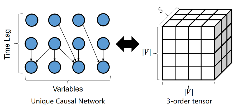
Figure 1: Tensor-based representation of UCN.

Unique Causal Network Model

Consider a network $\mathcal{G}=(\mathbf{V},\mathbf{E})$. The adjacency $A\in\mathbb{R}^{|\mathbf{V}|\times|\mathbf{V}|\times S}$ matching $\mathcal{G}$ is a real 3-order tensor recording the weights of edges. The weight $A_{jis}$ represents the causal effect $X_{j,t-s}\rightarrow X_{i,t}$ with time lag $s$. Then, it can be concluded that $\mathcal{G}$ is a DAG as shown in Fig. 1.

Proposition 1 (Acyclic).

$\mathcal{G}$ is a DAG.

Proof.

If $\mathcal{G}$ is not a DAG, there is at least one path $\mathbf{p}$ which is a cycle. Then, for any two different nodes $X,Y\in\mathbf{p}$, there must be two different path $X\rightarrow\dots\rightarrow Y$ and $Y\rightarrow\dots\rightarrow X$ without intersection except for them two. Then, $X$ is the direct or indirect cause of $Y$, and the direct or indirect effect of $Y$ at the same time. This is contradictory to the temporal assumption. ∎

Thus, due to the acyclic property, the assumptions of Markov property and faithfulness (see Definition 2 and Definition 3) can also be applied to our model.

Then, the equivalence of d-separation (equal to conditional independence), zero transfer entropy and time-series unpredictability can be inferred as the following proposition.

Proposition 2 (Causal equivalence).

Given the causal network $\mathcal{G}$, then the d-separation in $\mathcal{G}$, zero transfer entropy and time-series unpredictability in the system $\mathcal{S}$ are equivalent, which can be represented as

$$X\perp\!\!\!\perp_{\mathcal{G}}Y|\mathbf{Z}\iff\mathcal{T}_{Y\rightarrow X|\mathbf{Z}}=0\iff\mathcal{F}_{Y\rightarrow X|\mathbf{Z}}=0,$$ (11)

for any possible variable $Y$ preceding the target variable $X$, and $\mathbf{Z}$ is the set of some variables preceding $X$ as conditional set.

To prove this proposition, two lemmas need to be introduced first as follows.

Lemma 1.

For a variable $X$ and another variable $Y$ preceding $X$, $X\perp\!\!\!\perp_{\mathcal{G}}Y|\mathbf{Z}$ if and only if the transfer entropy $\mathcal{T}_{Y\rightarrow X|\mathbf{Z}}=0$, where $\mathbf{Z}$ is the conditional set of $X$ and $\mathbf{Pa}_{X}\subseteq\mathbf{Z}$.

Proof.

Given the variables $X$ and $Y$, then $X\perp\!\!\!\perp_{\mathcal{G}}Y|\mathbf{Z}\Rightarrow X\perp\!\!\!\perp Y|\mathbf{Z}$ because of the Markov property of $\mathcal{G}$. Thus $\mathcal{T}_{Y\rightarrow X|\mathbf{Z}}=H(X|\mathbf{Z})-H(X|\mathbf{Z},Y)=0$. On the other hand, if $\mathcal{T}_{Y\rightarrow X|\mathbf{Z}}=0$, then $X\perp\!\!\!\perp Y|\mathbf{Z}$. Thus, $X\perp\!\!\!\perp Y|\mathbf{Z}\Rightarrow X{\perp\!\!\!\perp}_{\mathcal{G}}Y|\mathbf{Z}$ due to the faithfulness. ∎

Lemma 2.

For a variable $X$ and another variable $Y$ preceding $X$, the transfer entropy $\mathcal{T}_{Y\rightarrow X|\mathbf{Z}}=0$ if and only if $\mathcal{F}_{Y\rightarrow X|\mathbf{Z}}=0$, where $\mathbf{Z}$ is a conditional set of $X$.

Proof.

Barnett and Bossomaier (2012) has proved a theorem to show that $\mathcal{T}_{Y\rightarrow X}=0$ if and only if $\mathcal{F}_{Y\rightarrow X}=0$ in a bivariate nonlinear system as stated in the background section. To prove lemma 2 under the circumstance of system $\mathcal{S}$, we provide a similar but not same proof in the conditional case as follows.

Given the variables $X$, $Y$ and $\mathbf{Z}$ with their continuous samples $x^{(k)}$, $y^{(k)}$ and $\mathbf{z}^{(k)}$. $x^{(k)}$ is considered as a sequence with $k$ samples collected from a segment of stochastic process in system $\mathcal{S}$, namely as $x^{(k)}=\{x_{1},\dots,x_{k}\}$, and the other two are the same. Note that $x^{(k)},y^{(k)},\mathbf{z}^{(k)}$ do not consider the subscript because they have the property of time delay. For the joint process $(X,Y,\mathbf{Z})$ in general, each joint samples of $(x^{(k)},y^{(k)},\mathbf{z}^{(k)})$ can be supposed to be ergodic. Then, it is natural to define the transfer entropy as

$$\mathcal{T}_{Y\rightarrow X|\mathbf{Z}}=H(X|\mathbf{Z})-H(X|Y,\mathbf{Z}).$$ (12)

Furthermore, the prediction model containing parameters can be defined as

$$f(x|y,\mathbf{z};\bm{\theta})=P(X|Y,\mathbf{Z};\bm{\theta}),$$ (13)

where $f$ is a conditional probability distribution function in terms of the joint samples $(x^{(k)},y^{(k)},\mathbf{z}^{(k)})$. The model $f$ is assumed to be identifiable and the parameters are assumed to be unique such that $f(\cdot|\cdot;\bm{\theta}_{1})\neq f(\cdot|\cdot;\bm{\theta}_{2})$ for $\bm{\theta}_{1}\neq\bm{\theta}_{2}$. Thus, the unique true parameter $\bm{\theta}^{*}$ satisfy

$$f(x|y,\mathbf{z};\bm{\theta}^{*})=P(X|Y,\mathbf{Z};\bm{\theta}^{*})=P(X|Y,\mathbf{Z}).$$ (14)

Thus, considering the ergodic assumption (Walters 2000) that $x_{t}$ is only up to $y_{t}$ and $\mathbf{z}_{t}$ for any $t=1,\dots,k$ in $f$, the likelihood for $\bm{\theta}$ can be written as

$$\quad\mathcal{L}_{k}(\mathbf{\theta}|x^{(k)},y^{(k)},\mathbf{z}^{(k)})$$ (15)

$$= P(x^{(k)},y^{(k)},\mathbf{z}^{(k)};\bm{\theta})$$

$$= P(x_{k}|x^{(k-1)},y^{(k)},\mathbf{z}^{(k)};\bm{\theta})$$

$$*P(y_{k},\mathbf{z}_{k}|x^{(k-1)},y^{(k-1)},\mathbf{z}^{(k-1)};\bm{\theta})$$

$$*P(x^{(k-1)},y^{(k-1)},\mathbf{z}^{(k-1)};\bm{\theta})$$

$$= f(x_{k}|y_{k},\mathbf{z}_{k};\bm{\theta})q(y_{k},\mathbf{z}_{k})\mathcal{L}_{k-1}$$

$$= \prod_{t=1}^{k}f(x_{t}|y_{t},\mathbf{z}_{t};\bm{\theta})q(y_{t},\mathbf{z}_{t}),$$

where $P(x_{t}|x^{(t-1)},y^{(t)},\mathbf{z}^{(t)};\bm{\theta})=f(x_{t}|x^{(t-1)},y^{(t)},\mathbf{z}^{(t)};\bm{\theta})=f(x_{t}|y_{t},\mathbf{z}_{t};\bm{\theta})$. Moreover, the parameter set $\bm{\theta}$ only affects $X$, thus $P(y_{t},\mathbf{z}_{t}|x^{(t-1)},y^{(t-1)},\mathbf{z}^{(t-1)};\bm{\theta})$ can be simplified as a distribution $q(y_{t},\mathbf{z}_{t})$, which does not equal to zero almost everywhere and not refer to $\bm{\theta}$. Then, to maximize the likelihood $\mathcal{L}_{k}$, the average log-likelihood is obtained as

$$\ell(\mathbf{\theta}|x^{(k)},y^{(k)},\mathbf{z}^{(k)}) =\frac{1}{k}\log\mathcal{L}_{k}(\mathbf{\theta}|x^{(k)},y^{(k)},\mathbf{z}^{(k)})$$ (16)

$$\sim\frac{1}{k}\sum_{t=1}^{k}\log f(x_{t}|y_{t},\mathbf{z}_{t};\bm{\theta}).$$

Apparently, the unique parameter $\theta^{*}$ for the prediction model $f$ can always be obtained as $k\rightarrow\infty$. Thus, according to the Birkhoff-Khinchin ergodic theorem (Walters 2000) and the Eq. (14),

$$\ell\stackrel{{\scriptstyle a.s}}{{\longrightarrow}}E[\log f(x|y,\mathbf{z};\bm{\theta})],$$ (17)

and then

$$E[\log f(x|y,\mathbf{z};\bm{\theta})]\stackrel{{\scriptstyle a.s}}{{\longrightarrow}}-H(X|Y,\mathbf{Z})$$ (18)

as $k\rightarrow\infty$.

Then, a nested null model can be defined as $H_{0}:\bm{\theta}\in\bm{\Theta}_{0}$. $\bm{\Theta}_{0}=\{\bm{\theta}\in\bm{\Theta}|X$ are indenpendent of $Y$ given $\mathbf{Z}\}$, and $\bm{\Theta}_{0}\subseteq\bm{\Theta}$, which is the full parameter set. Then, the likelihood ratio can be defined as

$$\Lambda(x^{(k)},y^{(k)},\mathbf{z}^{(k)})=\frac{\mathcal{L}_{k}(\hat{\mathbf{\theta}}_{0}|x^{(k)},y^{(k)},\mathbf{z}^{(k)})}{\mathcal{L}_{k}(\hat{\mathbf{\theta}}|x^{(k)},y^{(k)},\mathbf{z}^{(k)})},$$ (19)

where $\hat{\mathbf{\theta}}_{0}$ and $\hat{\mathbf{\theta}}$ are the Maximum likelihood estimators for $\bm{\Theta}_{0}$ and $\bm{\Theta}$, respectively. It is intuitive that $\Lambda(x^{(k)},y^{(k)},\mathbf{z}^{(k)})$ measures the dependence degree of predicting $X$ given $Z$ to $Y$. Thus, the degree of predictability can be defined as

$$\mathcal{F}_{Y\rightarrow X|\mathbf{Z}}=-\frac{1}{k}\log\Lambda(x^{(k)},y^{(k)},\mathbf{z}^{(k)}),$$ (20)

Where $\mathcal{F}_{Y\rightarrow X|\mathbf{Z}}\in[0,+\infty)$. Then, $\mathcal{F}_{Y\rightarrow X|\mathbf{Z}}\stackrel{{\scriptstyle a.s}}{{\longrightarrow}}\mathcal{T}_{Y\rightarrow X|\mathbf{Z}}$ as $k\rightarrow\infty$ obviously according to Eq. (12), Eq. (17) and Eq. (18). Thus, $\mathcal{F}_{Y\rightarrow X|\mathbf{Z}}$ and $\mathcal{T}_{Y\rightarrow X|\mathbf{Z}}$ have the same result based on the chi-square test (Barnett and Bossomaier 2012), namely $\mathcal{T}_{Y\rightarrow X|\mathbf{Z}}=0$ if and only if $\mathcal{F}_{Y\rightarrow X|\mathbf{Z}}=0$. ∎

Consequently, Proposition 2 is correct with no more proof needed since the Lemma 1 and the Lemma 2. It is an important conclusion that the causal connections in $\mathcal{G}$ imply the information of predictability.

Next, it is important to know which variables have the key influence to predict the state of target variable $X$. Starting from the concept of the parents $\mathbf{Pa}_{X}$ to $X$, it can be concluded that all variables in $\mathbf{Pa}_{X}$ precede $X$ because of the temporal assumption. And then, any variable in $\mathbf{Pa}_{X}$ assists in prediction as the following proposition states.

Proposition 3.

$\forall Y\in\mathbf{Pa}_{X}$, the variable $Y$ satisfy $\mathcal{F}_{Y\rightarrow X|\mathbf{Pa}_{X}\backslash\{Y\}}>0$.

Proof.

For any variable $Y\in\mathbf{Pa}_{X}$, there is no variable set that can d-separate $X$ and $Y$. Thus, it is natural to induce $\mathcal{F}_{Y\rightarrow X|\mathbf{Pa}_{X}\backslash\{Y\}}>0$ from $Y\not\!\perp\!\!\!\perp_{\mathcal{G}}X|\mathbf{Pa}_{X}\backslash\{Y\}$ based on the Proposition 2. ∎

This proposition is often used to search the skeleton of the Bayesian network globally by conditional independence test (Spirtes et al. 2000; Kalisch and Bühlman 2007). But only by conditional independence test, the structure $X\rightarrow Y\rightarrow Z$, $X\leftarrow Y\leftarrow Z$ and $X\leftarrow Y\rightarrow Z$ can not be distinguished in various Markov equivalence classes of Bayesian network (Verma, Pearl et al. 1991). In the UCN, this issue can be addressed because of the temporal assumption, as the following propositon states.

Proposition 4.

$\forall Y$ preceding $X$ and $Y\notin\mathbf{Pa}_{X}$, the variable $Y$ satisfy $\mathcal{F}_{Y\rightarrow X|\mathbf{Pa}_{X}}=0$.

Proof.

For any variable $Y$ preceding $X$ and $Y\notin\mathbf{Pa}_{X}$, $Y\perp\!\!\!\perp_{\mathcal{G}}X|\mathbf{Pa}_{X}$ because all paths from $Y$ to $X$ are blocked by $\mathbf{Pa}_{X}$ in $\mathcal{G}$. Due to $\mathbf{Pa}_{X}=\mathbf{Pa}_{X}\backslash\{Y\}$, it can be concluded that $Y\perp\!\!\!\perp_{\mathcal{G}}X|\mathbf{Pa}_{X}\backslash\{Y\}$. Thus $\mathcal{F}_{Y\rightarrow X|\mathbf{Pa}_{X}\backslash\{Y\}}=0$ according to the Proposition 2. ∎

Then, it can be directly obtained that

Corollary 1.

$\forall Y$ preceding $X$, $Y\notin\mathbf{Pa}_{X}$ if and only if $\mathcal{F}_{Y\rightarrow X|\mathbf{Pa}_{X}\backslash\{Y\}}=0$.

This corollary is important to design the search algorithm to learn causal structure of $\mathcal{G}$. Next,

Proposition 5.

For any nested variable set $\mathbf{M}\supseteq\mathbf{Pa}_{X}$, and all variables in $\mathbf{M}$ precede $X$, then $\forall Y\in\mathbf{V}\backslash\mathbf{M}\cup\{X\}$, $Y\perp\!\!\!\perp_{\mathcal{G}}X|\mathbf{M}$, namely $\mathcal{F}_{Y\rightarrow X|\mathbf{M}}=0$.

Proof.

Let $\mathbf{M}\supseteq\mathbf{Pa}_{X}$ and all variables in $\mathbf{M}$ precede $X$. For any selected $Y\in\mathbf{V}\backslash\mathbf{M}\cup\{X\}$, then $Y\notin\mathbf{Pa_{X}}$. According to Proposition 4, we have $\mathcal{F}_{Y\rightarrow X|\mathbf{Pa}_{X}}=0$. And then $Y\perp\!\!\!\perp_{\mathcal{G}}X|\mathbf{Pa}_{X}$ due to the causal equivalence, which means $\mathbf{Pa}_{X}$ blocks any paths between $X$ and $Y$. Thus $\mathbf{M}$ also blocks any paths between $X$ and $Y$ because $\mathbf{M}\supseteq\mathbf{Pa}_{X}$, namely $Y\perp\!\!\!\perp_{\mathcal{G}}X|\mathbf{M}$. ∎

Then, the following corollary can be obtained with few proofs.

Corollary 2.

For any variable $X$ in $\mathcal{G}$, $\mathbf{Pa}_{X}=\mathbf{M}_{X}$, which is the Markov blanket containing all knowledge for predicting $X$.

Proof.

According to the Proposition 5, $\mathbf{Pa}_{X}$ is the minimal variable set of $\mathbf{M}$, which satisfied Definition 5. Thus, $\mathbf{Pa}_{X}=\mathbf{M}_{X}$. ($\mathbf{M}_{X}$ must contain $\mathbf{Pa}_{X}$, otherwise $\exists Y$ precedes $X$, $Y\in\mathbf{Pa}_{X}$, $Y\notin\mathbf{M}_{X}$, and then $Y\not\!\perp\!\!\!\perp_{\mathcal{G}}X|\mathbf{M}_{X}$, which is not satisfied Definition 5) ∎

Consequently, the predictability of the target variable $X$ is only up to its causal parents $\mathbf{Pa}_{X}$ in $\mathcal{G}$. Thus, the decomposability of the causal network $\mathcal{G}$ can be explored

Proposition 6 (Decomposability).

The causal network $\mathcal{G}$ can be decomposed into $n$ subgraphs $\mathcal{G}_{i,t}=(\mathbf{V},\mathbf{E}_{i,t})$ for simultaneous variables $X_{i,t},i=1,\dots,n$. Then, the d-separation in $\mathcal{G}$ is same as that in $\mathcal{G}_{i,t}$, namely $\perp\!\!\!\perp_{\mathcal{G}}\iff~{}\perp\!\!\!\perp_{\mathcal{G}_{i,t}}$.

Proof.

Refer to Corollary 2, the predictability for each target variables $X_{i,t},i=1,\dots,n$ is only decided by their parents $\mathbf{Pa}_{i}$. And, there must be no connection between these variables at the same time $t$ because of the temporal assumption. Thus, $\mathcal{G}$ can be decomposed into $n$ subgraphs $\mathcal{G}_{i,t}=(\mathbf{V},\mathbf{E}_{i,t})$ where $\mathbf{E}_{i,t}$ is the directed connections from each variables of $\mathbf{Pa}_{i}$ to $X_{i}$. To put it another way, $\mathcal{G}$ is the linear combination of all $\mathcal{G}_{i,t}$. Furthermore, $\perp\!\!\!\perp_{\mathcal{G}}\iff\perp\!\!\!\perp_{\mathcal{G}_{i,t}}$ is trivial to see in Fig. 2. ∎

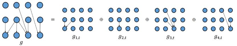
Figure 2: The way to decompose UCN and combine all subgraphs. $\bigoplus$ represents linear combination.

Next, the uniqueness of the causal network $\mathcal{G}$ can be further proved as follows.

Proposition 7 (Uniqueness).

The causal network $\mathcal{G}$ is unique.

Proof.

According to the principle of decomposability, we have $n$ subgraphs $\mathcal{G}_{i,t}$ of $\mathcal{G}$. In $\mathcal{G}_{i,t}$, the parents of the target variable $X_{i,t}$ is unique. we can first prove it.

Let $X$ be any target variable $X_{i,t}$. Then, $\mathbf{Pa}_{X}$ and $\widetilde{\mathbf{Pa}}_{X}$ are both the parents of $X$ in $\mathcal{G}_{i,t}$ and $\widetilde{\mathcal{G}}_{i,t}$, respectively. $\forall Y\in\widetilde{\mathbf{Pa}}_{X}$, no variable set $\mathbf{Z}$ excluding $X$ and $Y$, which contains the set $\mathbf{Pa}_{X}\backslash\{Y\}$, satisfying $Y\not\!\perp\!\!\!\perp_{\widetilde{\mathcal{G}}_{i,t}}X|\mathbf{Z}$. Thus, $Y\not\!\perp\!\!\!\perp_{\widetilde{\mathcal{G}}_{i,t}}X|\mathbf{Pa}_{X}\backslash\{Y\}$, and then $Y\not\!\perp\!\!\!\perp_{{\mathcal{G}}_{i,t}}X|\mathbf{Pa}_{X}\backslash\{Y\}$ because of $\perp\!\!\!\perp_{\widetilde{\mathcal{G}}_{i,t}}\iff\perp\!\!\!\perp_{\mathcal{G}}\iff\perp\!\!\!\perp_{\mathcal{G}_{i,t}}$ (see decomposability). Then, $Y\in\mathbf{Pa}$ can be concluded from the Corollary 1 and the causal equivalence. Thus, $\widetilde{\mathbf{Pa}}_{X}\subseteq\mathbf{Pa}_{X}$. In a similar way, $\widetilde{\mathbf{Pa}}_{X}\supseteq\mathbf{Pa}_{X}$ can be also obtained. Thus, $\mathbf{Pa}_{X}=\widetilde{\mathbf{Pa}}_{X}$. Thus, the $\mathcal{G}_{i,t}$ is same as $\widetilde{\mathcal{G}}_{i,t}$.

Consequently, the causal network $\mathcal{G}$ is unique because all subgraphs $\mathcal{G}_{i,t}$ are unique and $\mathcal{G}$ is just the linear combination of multiple unique subgraphs. ∎

The property of uniqueness guarantees that UCN avoids the issue of Markov equivalence class, which enables UCN to be more accurate and explainable.

Higher-order Causal Entropy Algorithm

To identify the structure of UCN, a novel algorithm based on the principle of higher-order causal entropy, namely HCE, is proposed. Causal entropy is a special case of transfer entropy (Sun, Taylor, and Bollt 2015). It is measured by nearest-neighbors entropy estimator (Kraskov, Stögbauer, and Grassberger 2004) with no stationary assumption. The pseudocode of HCE is shown in the following Algorithm 1.

First of all, due to the decomposability property (see Proposition 6), the network can be decomposed into $n$ subgraphs. These subgraphs can be identified respectively and stacked to be a complete network finally. Thus, HCE algorithm can be decomposed into $n$ child processes. Each child process searches causal parents $\mathbf{Pa}_{i}$ for target variable $X_{i}$, in a distributed way instead of $n$-times sequential iterations.

Then, each child process can be decomposed into two modules by parameters $\tau_{max},\alpha$ and $\beta$. In the first module, for target variable $X_{i}$, HCE calculates the causal entropy of each historical variable and each time delay $\tau=1,\dots,\tau_{max}$. It saves part of variables from the given conditional set and finally obtains the possible $\mathbf{Pa}_{i}$. In the second module, HCE removes spurious causation from $\mathbf{Pa}_{i}$ and the subgraph is obtained at the end. $\alpha$ and $\beta$ are both used to control the bound of zero causal entropy according to Corollary 1. If the obtained value of causal entropy is less than $\alpha$ or $\beta$, the value will be approximated to be zero. Thus, the obtained $\mathbf{Pa}_{i}$ becomes narrower with bigger $\alpha$ and $\beta$. Finally, the network can be obtained by combining all subgraphs.

Furthermore, time complexity of HCE is $\mathcal{O}(n^{3}\tau_{max})$. The main computational cost comes from searching causal parents for each variable at time $t$ and estimating causal entropy for each possible edge. In HCE algorithm, the time complexity of searching causal parents is $\mathcal{O}(n\tau_{max})$ because all historical variables need to be traversed. Then, note that HCE algorithm can be distributed. Thus, the time is calculated only for each variable, and the time to combine all subgraphs is $\mathcal{O}(1)$, that can be ignored. Meanwhile, the so-called KSG estimator (Kraskov, Stögbauer, and Grassberger 2004) is adopted to measure causal entropy with time complexity $\mathcal{O}(n^{2})$ in worst case. But it can be accelerated by using KD-tree neighbor search.

Input: Observation set $\mathbf{U}=\{X_{1},\dots,X_{n}\}$ and maximum time lag $\tau_{max}$.

Output: An UCN $\mathcal{G}$.

1

2for $i=1,\dots,n$ do

3       Initialize the causal parent set $\mathbf{Pa}_{i}=\varnothing$;

4       for $\tau=1,\dots,\tau_{max}$  do

5             Initialize condition set $\mathbf{Z}=\{X_{1,\tau},\dots,X_{n,\tau}\}$;

6             for $j=1,\dots,n$ do

7                   Let $\mathcal{T}_{X_{j,\tau}\rightarrow X_{i}|\mathbf{Z}\backslash\{X_{j,\tau}\}}=H(X_{i}|\mathbf{Z}\backslash\{X_{j,\tau}\})-H(X_{i}|\mathbf{Z})$;

8                   if $\mathcal{T}_{X_{j,\tau}\rightarrow X_{i}|\mathbf{Z}\backslash\{X_{j,\tau}\}}>\alpha$ then

9                         append $X_{j,\tau}$ into $\mathbf{Pa}_{i}$;

10                  else

11                         remove $X_{j,\tau}$ from $\mathbf{Z}$;

12                  

13            

14      

15      for each $Y\in\mathbf{Pa}_{i}$ do

16             Let $\mathcal{T}_{Y\rightarrow X_{i}|\mathbf{Pa}_{i}\backslash\{Y\}}=H(X_{i}|\mathbf{Pa}_{i}\backslash\{Y\})-H(X_{i}|\mathbf{Pa}_{i})$;

17             if $\mathcal{T}_{Y\rightarrow X_{i}|\mathbf{Pa}_{i}\backslash\{Y\}}<\beta$ then

18                   remove $Y$ from $\mathbf{Pa}_{i}$;

19            

20      

Construct the network $\mathcal{G}$ with $\mathbf{Pa}_{1},\dots,\mathbf{Pa}_{n}$;

Algorithm 1 Higher-order Causal Entropy Algorithm

Experiments

Synthetic Data

In the experiments, the performance of HCE algorithm is tested at synthetic data generated from the UCN. For example, as shown in Fig. 3, $f_{1},f_{2}$ are both functions, defined as $f_{1}(x)=x$ and $f_{2}(x)=x+5x^{2}\exp^{-\frac{x^{2}}{20}}$. The state of variable at time $t$ is certainly calculated by the historical states of all variables, such that $x_{1,t}=0.2f_{2}(x_{1,t-1})+0.3f_{1}(x_{env,t-1})+\mathcal{N}(0,1)$, where the noise is assumed to be normal distribution in general. Apparently, the environment variable $X_{env}$ is the common parent for variable $X_{1}$ and variable $X_{4}$, and it is not affected by any other variables.

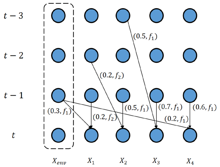
Figure 3: An example of the UCN

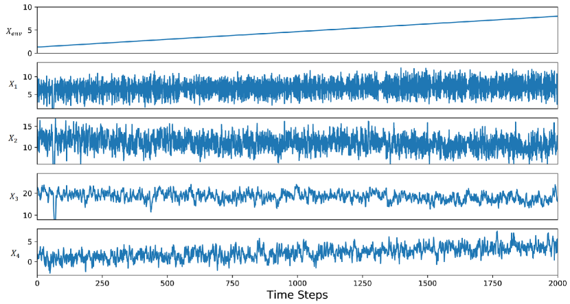
Figure 4: Generated time series of five variables with 2000 time steps

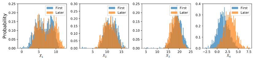
Figure 5: Dataset shift of the four observation variables

Thus, to generate nonstationary data in a simple way, the state of environment variable $X_{env}$ is assumed to be a linear increasing sequence as shown in Fig. 4. It can be seen that the evolution curve of $X_{env}$ is in the range of $1.3\sim 8.0$ with 2000 time steps. At the same time, the other observation variables are also presented in Fig. 4. They all fluctuate in different and limited ranges, and have no property of periodicity.

To reveal the nonstationarity in the generated time series, the distributions of the four observation variables within the first 1000 time steps and that within the later 1000 time steps are also shown in Fig. 5, respectively. It is clear that the dataset shift of all variables occurs to some extents when time segments change. Especially for variable $X_{4}$, the statistical distribution over the first 1000 steps is greatly shift to the left of distribution over the later 1000 steps. Thus, if we adopt some regression methods, such as granger causality (Granger 1969), to detect causality between these variables, the obtained results of regression will be time-varying because of time-varying distribution.

Moreover, all synthetic data is randomly generated from many UCNs like Fig. 3, and we will not list them all here. But in practice, their network size $n$ and number of edges are specially designed for different scenarios. The number of edges is at least twice the network size and the sample size is fixed to be 2000 in all scenarios.

Evaluation Metrics

In the experiments, two indices are adopted to measure the performance of model, including true positive rate (TPR) and false positive rate (FPR). They are defined as

$$TPR =\frac{true~{}positive}{true~{}positive+false~{}negative},$$ (21)

$$FPR =\frac{false~{}positive}{false~{}positive+true~{}negative}.$$

Results

To test the performance of HCE algorithm, GC (Granger 1969), CCM (Sugihara et al. 2012) and PCMCI (Runge et al. 2019) are selected for comparison. In the experiments, the actual UCN is hidden first, and then the network structure needs to be reconstructed by these algorithms. The TPR and FPR are both calculated after the running of these algorithms on the synthetic data as shown in Fig. 3. The parameters of HCE are set as that $\tau_{max}=5,\alpha=0.01$ and $\beta=0.02$. Then, the receiver operating characteristic (ROC) curve is drawn. But note that the scores calculated for ROC curve have different representations in each algorithm. In HCE, the causal entropy of each edge is recorded, and finally normalized into range of 0 and 1 by min-max scaling.

Figure 6: The ROC curve of HCE and other algorithms.

Figure 7: The accuracy of HCE and other algorithms with different network size.

As shown in Fig. 6, the ROC curve of HCE overall covers the curves generated from other algorithms, which means the area under curve (AUC) of HCE is higher than that of other algorithms. Thus, it can be concluded that HCE algorithm achieves better generalization at different classification thresholds in nonstationary time series when the network size is 5.

Furthermore, the performance of HCE algorithm is tested on dataset with bigger network size. As shown in Fig. 7, it is clear that HCE algorithm performs generally better than other baseline algorithms with increasing network size. Note that all results for boxplot are tested on the dataset generated from UCNs with different network sizes and different network structures. Besides, the data generation processes are executed at least 20 times to eliminate test errors.

For all algorithms, the FPRs are fixed to be below 0.1 except for GC. Due to the bad adaption for nonstationary time series, GC achieves higher TPRs and FPRs at the same time. The results have large variances at each running time. For the other three algorithms, the FPRs decrease as the network size increases. This is because the increasing network size leads to the exponential increase of negative edges, which makes imbalance between the false positives and the true negatives.

As shown in Fig. 7, the TPR of HCE algorithm gradually decreases with the increase of network size, but it is still higher than that of PCMCI with the almost same FPR. The decreasing performance of HCE results from the decreasing accuracy of causal entropy estimation in scenarios with lots of variables. But it can be improved by other estimator (e.g., Belghazi et al. 2018) with a little more time consumption. Consequently, without loss of generality, HCE can better detect causality from nonstationary time series compared to the other widely accepted baseline algorithms.

Conclusion and Future Work

In this paper, UCN model is proposed to address the issue of Markov equivalence class. Some proofs are provided to explicitly show the uniqueness property of UCN, which guarantees the identified network structure is unique. Furthermore, the decomposability of UCN is also proved. Based on this property, HCE algorithm is designed to identify the structure of UCN in a distributed way. HCE algorithm identifies the causality by an improved nearest-neighbors entropy estimator, which works well in nonstationary time series. Lots of experiments are conducted to test the performance of HCE algorithm on synthetic data, compared with the other algorithms, including GC, CCM and PCMCI. The results show that HCE algorithm can achieve state-of-the-art accuracy even though the time series are nonstationary.

In the future, we will focus on improving the accuracy of algorithm when the network size is large. For example, the method like (Belghazi et al. 2018) to estimate mutual information based on neural network can be used to replace the nearest-neighbors entropy estimator with a little more time consumption. The method using neural network like transformer (Vaswani et al. 2017) can also be adopted to identify the weight tensor of UCN via an end-to-end way.

Furthermore, we will focus on the issue of causal inference based on the proposed UCN-based structural causal model (SCM). In general, SCM-based causal inference has three steps, including identifying causal graph (BN-like DAG or others), intervention, and counterfactual (Peters, Janzing, and Schölkopf 2017). UCN can be an alternative network model for the BN. To do intervention and infer counterfactual on UCN-based SCM, one may reconstruct intervened distribution by copula-based methods (Cherubini, Luciano, and Vecchiato 2004; Ibragimov 2009), or convert a UCN-based SCM into a stochastic differential equation and solve it, like (Ness, Paneri, and Vitek 2019). The bottleneck may be the way how to define the tools of intervention, and how to expand the application to the scenarios of higher-order Markov process.

Consequently, The feasibility of above ideas will be tested in the future. We believe that UCN can be expanded to be a more general framework for describing causality in complex system.