How to train your draGAN: A task oriented solution to imbalanced classification

Abstract

The long-standing challenge of building effective classification models for small and imbalanced datasets has seen little improvement since the creation of the Synthetic Minority Over-sampling Technique (SMOTE) over 20 years ago. Though GAN based models seem promising, there has been a lack of purpose built architectures for solving the aforementioned problem, as most previous studies focus on applying already existing models. This paper proposes a unique, performance-oriented, data-generating strategy that utilizes a new architecture, coined draGAN, to generate both minority and majority samples. The samples are generated with the objective of optimizing the classification model’s performance, rather than similarity to the real data. We benchmark our approach against state-of-the-art methods from the SMOTE family and competitive GAN based approaches on 94 tabular datasets with varying degrees of imbalance and linearity. Empirically we show the superiority of draGAN, but also highlight some of its shortcomings.
All code is available on: https://github.com/LeonGuertler/draGAN

1 Introduction

Numerous real-world business applications of Machine Learning are based on tabular data [1, 2] which is often imbalanced [1]. This poses a significant problem to Machine Learning models, as they will oftentimes only fit the majority class, neglecting the minority class [3, 4]. Alleviation of this problem can be achieved on both the data-level and the model-level. Whilst model-level approaches tend to focus on complex architectures or bespoke loss functions that pay more attention to the minority class [5, 6], data-level approaches are more general and focus on sampling methods [7], data augmentation [8] and data generation [6, 9, 10, 11, 12], which makes them compatible with any classification model. SMOTE [9], the “de facto” standard for learning from imbalanced data, even though performing well in practice, is not able to effectively extend the training field [13]; generated samples lack diversity [13] and it does not take decision boundaries into account. Furthermore, any data points generated are solely based on the samples in the minority class, which means that the model misses out on valuable information about the data’s distribution. GAN based approaches, especially cWGAN [11], address the above issues but take substantially longer than SMOTE to converge. Moreover, one problem with using GANs to generate a batch of training samples for the classification model is that each data point is generated independently. Therefore, they might not be well distributed in the sample space and thus skew the classification model. However, the biggest shortcoming of both approaches is that they focus on generating synthetic data points that are similar to the real data, rather than data points that lead to the best classification performance.
We propose a novel GAN based architecture, coined draGAN (Deep Reinforcement Augmented Generative Adversarial Network), that directly addresses the aforementioned problems. Namely, model collapse is solved by using one-dimensional convolutional layers in the Generator to map a single Gaussian noise vector to a whole training batch of samples, ensuring coherence; the objective of priming generated data points on the performance of the classification model is realized by using the Discriminator, in our work referred to as Critic, to estimate the performance (i.e. AUC) the classification model would achieve on the training data if it were trained on the generated data points.

Our contribution can be summarized as follows:

• We create a new Generator architecture that generates full, coherent, training batches with every forward pass.

• We propose an alternative function of the adversarial, using it to estimate the training value of the generated data points, and therefore effectively extend its purpose into a domain beyond simply estimating the realisticity of generated data.

2 Related Work

In SMOTE [9], new datapoints ($x_{new}$) are generated by randomly sampling from the minority class ($x_{i}$) and creating a linear interpolation of its features with one of its nearest minority class neighbours ($x_{j}$).

$$x_{new}=x_{i}+\epsilon*(x_{j}-x_{i});\text{where}\ \epsilon\sim U(0,1)$$ (1)

This concept has be built upon by hundreds of similar algorithms and most of them were recently benchmarked by [14], where the authors point out that even though overall polynom-fit-SMOTE [15] is the best one, the performance gain over SMOTE is marginal. Polynom-fit-SMOTE generates new data points along line segments between minority class samples that are connected via one of the four topological techniques (”bus”, ”star”, ”mesh” and ”polynom”). This means that generated data points will be more scattered as compared to SMOTE. Though [15] concludes that the ”star” and ”mesh” strategies perform best, [14] finds that all four strategies perform similarly. In this work, we will utilize the ”star” strategy.

Similarly to SMOTE, MixUp [16] proposes a linear interpolation of features of two data points, however, these data points don’t need to be from the same class or cluster, and hence the labels are also interpolated (2 and 3 respectively).

$$x_{new}=\lambda x_{i}+(1-\lambda)x_{j}$$ (2)

$$y_{new}=\lambda y_{i}+(1-\lambda)y_{j}$$ (3)

Where $\lambda\sim\text{Beta}(\alpha,\alpha)$, for $\alpha\in(0,\infty)$.
However, in the context of binary classification with out of the box models, the label has to be in a discrete format, which we enforce by rounding.
Because of the nature of these algorithms, they are not able to effectively extend the training field [13], generated samples can lack diversity [13] and decision boundaries are not taken into consideration. Moreover, they do not attempt to accurately approximate the probability distribution of the positive samples, which is an issue that GANs address.

Since its inception, GAN [10] has shown an astonishing capability of generating realistic samples for different, often high dimensional, data types [17, 18, 19, 20]. This popularity has resulted in the further development and application of the technique for other problems. Recently, [21] showed that GANs are a feasible solution to the imbalanced learning problem. However, they commonly suffer from unstable training [22], have no quantitative way of indicating convergence and, as applied in [21], do not make use of all the available data, as the network is trained solely on the minority class.

The instability of training and the absence of a convergence mechanism has successfully been addressed by a number of recent papers that utilize the Wasserstein-1 function as a loss for the discriminator, referred to as a critic in their work [23]. The discriminator has to lie within the space of 1-Lipschitz functions, which was enforced by clipping of weights. This both stabilizes the training process by providing more meaningful gradients and, since the Wasserstein-1 function measures the “distance”, shows whether the model converges. The method has been extended by [24] where the 1-Lipschitz constraint was enforced through gradient clipping, which further improves the quality of the gradients, especially when the initial solution is far from the target solution. However, it should be pointed out that in the context of using a Generative model to improve the classification accuracy of a secondary model, the Wasserstein-1 function does not indicate the convergence towards the actual goal of the model, namely, improving the classification performance of the secondary model, but rather indicates how similar the generated samples are to the original data.

The vanilla GAN model has no mechanism for generating samples with specific labels, except training the model exclusively on these labels. The idea of generating label specific data with GANs was first introduced by [25] where the Generator and Discriminator accept a one-hot encoded label vector in addition to the usual inputs (4). This architecture, coined cGAN, was successfully used to generate MNIST digits for given labels.

$$\min_{G}\max_{D}\mathbb{E}_{x\sim p_{\text{data}}(x)}[\log{D(x|y)}]+\mathbb{E}_{z\sim p_{\text{z}}(z)}[1-\log{D(G(z|y))}]$$ (4)

This method has been improved by an architecture coined AC-GAN [26] where, rather than providing two separate inputs, the Gaussian noise vector is augmented with a one-hot encoded label vector before being fed to the Generator. The Discriminator has two separate final layers, where one, the auxiliary head, predicts the label of the provided sample, and the other, the discriminatory head, whether the sample was generated. Whilst the Generator tries to maximize $L_{C}-L_{S}$, the Discriminator tries to maximize $L_{C}+L_{S}$.

$$L_{S}=\mathbb{E}[\log{P(S=\text{real}|X_{\text{real}})}]+\mathbb{E}[\log{P(S=\text{fake}|X_{\text{fake}})}]$$ (5)

$$L_{C}=\mathbb{E}[\log{P(C=c|X_{\text{real}})}]+\mathbb{E}[\log{(C=c|X_{\text{fake}})}]$$ (6)

cWGAN as used in [11] presents a combination of WGAN-GP [24] and an AC-GAN [26], by incorporating the AC loss. However, as they point out in their paper, their implementation deviates from the classic AC-GAN by using two separate networks for the discriminator and the auxiliary classifier, rather than merely two different heads. The architecture, which is optimized by (10), was purpose-built for oversampling tabular data for imbalanced learning and, to the best of our knowledge, is currently the state-of-the-art GAN based model for the aforementioned problem.

$$\text{Wasserstein-loss}=\mathbb{E}_{x\sim p_{\text{data}}(x)}[D(X)]-\mathbb{E}_{z\sim p_{z}}[D(G(z))]$$ (7)

$$\text{Gradient-penalty}=\lambda_{GP}\mathbb{E}_{\hat{x}\sim p_{\hat{x}}}[(\|\nabla_{\hat{x}}D(\hat{x})\|_{2}-1)^{2}]$$ (8)

$$\text{AC-loss}=\lambda_{\text{AC}}\mathbb{E}_{z\sim p_{z}}[\text{BCE}(\text{AC}(G(z))))]$$ (9)

$$\min_{G}\max_{D}(\text{Wasserstein-loss}-\text{Gradient-penalty}+\text{AC-loss})$$ (10)

One key issue that is neither addressed by cWGAN [11] nor SMOTE [9] is that for the purpose of building a high-performing classification model on an imbalanced dataset, the most important metric should be the model’s performance. Thus, we propose a GAN based architecture that incorporates a deep reinforcement learning agent to estimate the quality, in regards to improved classification performance, of each generated data point, called draGAN.

Before diving into the details of our proposed method (draGAN), we want to prevent any potential confusion by pointing out that this is a novel work, and in no way related to the DRAGAN algorithm developed by [27].

3 Methodology

The purpose of supervised learning algorithms is to predict a label y given an input x, for any pair that is jointly sampled from the distribution $p(x,y)$. This can be achieved by sampling a finite number of pairs $(x_{\tilde{\alpha}},y_{\tilde{\alpha}})_{\tilde{\alpha}\in\mathcal{A}}$ and minimizing

$$\mathcal{L}_{\mathcal{A}}(\theta)\equiv\sum_{\tilde{\alpha}\in\mathcal{A}}{\mathcal{L}(z(x_{\tilde{\alpha}};\theta),y_{\tilde{\alpha}})}$$ (11)

where $\tilde{\alpha}\in\mathcal{A}$ denotes inputs from the training set and $\mathcal{L}$ a loss function. The quality of the fitted parameters $\theta$ is commonly estimated on a number of test inputs, denoted as $\dot{\beta}\in\mathcal{B}$. The difference of the test loss and the training loss is referred to as the Generalization-error (12)

$$\mathcal{E}=\mathcal{L}_{\mathcal{B}}-\mathcal{L}_{\mathcal{A}}$$ (12)

In imbalanced classification problems, one class, referred to as the majority class, will be over-represented as compared to the other, referred to as minority class. This means that any equally weighted measures of success, such as accuracy, will be miss-leading. Thus, new measures that pay more attention to the minority class have been introduce [29, 30]. Inversely to the loss function, these measures indicate optimal performance at 1 and poor performance at 0.

Unfortunately, since these performance indicators are discrete, they can not directly be used for training. Furthermore, any equally weighted metric used for training, such as the ”de-facto” Negative Log-Likelihood Loss (13), will not guarantee a strictly inversely correlated performance on the discrete metrics, which will ultimately be used to validated the models success.

$$\mathcal{L}_{\mathcal{A}}(\theta)\equiv-\frac{1}{|\mathcal{A}|}\sum_{\tilde{\alpha}\in\mathcal{A}}{y_{\tilde{\alpha}}*log(z(x_{\tilde{\alpha}};\theta))+(1-y_{\tilde{\alpha}})*log(1-z(x_{\tilde{\alpha}};\theta))}$$ (13)

where $|\mathcal{A}|$ denote the cardinality (size) of the training set.

We justify this claim by computing the trivial solution with the lowest test loss and the corresponding $\text{F}_{1}\text{-Score}$.

We denote the weights corresponding to the proposed trivial solution as $\theta_{\text{trivial}}$. A trivial solution will have the best loss when a constant $\epsilon$ minimizes (14), for $\epsilon\in(0,1)$.

$$\mathcal{L}_{\mathcal{B}}(\theta_{\text{trivial}})$$

$$\equiv-\frac{1}{|\mathcal{B}|}\sum_{\dot{\beta}\in\mathcal{B}}{y_{\dot{\beta}}*log(z(x_{\dot{\beta}};\theta_{\text{trivial}}))+(1-y_{\dot{\beta}})*log(1-z(x_{\dot{\beta}};\theta_{\text{trivial}}))}$$

$$=-\frac{1}{|\mathcal{B}|}\sum_{\dot{\beta}\in\mathcal{B}}{y_{\dot{\beta}}*log(\epsilon)+(1-y_{\dot{\beta}})*log(1-\epsilon)}$$ (14)

$\epsilon$ can easily be determined by dividing (14) into a majority set ($\mathcal{B}_{\text{\tiny majority}}\subset\mathcal{B}$) and a minority set ($\mathcal{B}_{\text{\tiny minority}}\subset\mathcal{B}$), where $\mathcal{B}_{\text{\tiny minority}}=(\mathcal{B}_{\text{\tiny majority}})^{\complement}$ and hence $|\mathcal{B}_{\text{\tiny minority}}|+|\mathcal{B}_{\text{\tiny majority}}|=|\mathcal{B}|$.

$$\mathcal{L}_{\mathcal{B}}(\theta_{\text{trivial}})=-\frac{1}{|\mathcal{B}|}*(|\mathcal{B}_{\text{\tiny minority}}|*log(\epsilon)+|\mathcal{B}_{\text{\tiny majority}}|*log(1-\epsilon))$$ (15)

$$\frac{d\mathcal{L}_{\mathcal{B}}(\theta_{\text{trivial}})}{d\epsilon} =-\frac{1}{|\mathcal{B}|}*(\frac{|\mathcal{B}_{\text{\tiny minority}}|}{\epsilon}-\frac{|\mathcal{B}_{\text{\tiny majority}}|}{1-\epsilon})$$ (16)

$$\therefore\text{Minimum at }\epsilon=\frac{|\mathcal{B}_{\text{\tiny minority}}|}{|\mathcal{B}|}$$ (17)

The theoretical continuous confusion matrix can be expressed as.

		Predicted
		Yes	No
Actual	Yes	$0.5*\frac{|\mathcal{B}_{\text{\tiny minority}}|}{|\mathcal{B}|}*|\mathcal{B}|$	$0.5*(1-\frac{|\mathcal{B}_{\text{\tiny minority}}|}{|\mathcal{B}|})*|\mathcal{B}|$
	No	$0.5*\frac{|\mathcal{B}_{\text{\tiny minority}}|}{|\mathcal{B}|}*|\mathcal{B}|$	$0.5*(1-\frac{|\mathcal{B}_{\text{\tiny minority}}|}{|\mathcal{B}|})*|\mathcal{B}|$

Therefore, the $F_{1}\text{-Score}$ can be evaluated as

$$\text{Precision}_{\mathcal{B}} =\frac{0.5*\frac{|\mathcal{B}_{\text{\tiny minority}}|}{|\mathcal{B}|}*|\mathcal{B}|}{0.5*\frac{|\mathcal{B}_{\text{\tiny minority}}|}{|\mathcal{B}|}*|\mathcal{B}|+0.5*\frac{|\mathcal{B}_{\text{\tiny minority}}|}{|\mathcal{B}|}*|\mathcal{B}|}=0.5$$ (18)

$$\text{Recall}_{\mathcal{B}} =\frac{0.5*\frac{|\mathcal{B}_{\text{\tiny minority}}|}{|\mathcal{B}|}*|\mathcal{B}|}{0.5*\frac{|\mathcal{B}_{\text{\tiny minority}}|}{|\mathcal{B}|}*|\mathcal{B}|+0.5*(1-\frac{|\mathcal{B}_{\text{\tiny minority}}|}{|\mathcal{B}|})*|\mathcal{B}|}=\frac{|\mathcal{B}_{\text{\tiny minority}}|}{|\mathcal{B}|}$$ (19)

$$F_{1}\text{-Score} =\frac{2*0.5*\frac{|\mathcal{B}_{\text{\tiny minority}}|}{|\mathcal{B}|}}{0.5+\frac{|\mathcal{B}_{\text{\tiny minority}}|}{|\mathcal{B}|}}=\frac{|\mathcal{B}_{\text{\tiny minority}}|}{0.5*|\mathcal{B}|+|\mathcal{B}_{\text{\tiny minority}}|}=\frac{\epsilon}{0.5+\epsilon}$$ (20)

where (20) is a strictly increasing function with respect to the cardinality of $\mathcal{B}_{\text{\tiny minority}}$. This means that the higher the imbalance ratio, the lower the $F_{1}\text{-Score}$ of the trivial solution will be, which makes the function strictly correlated to the loss of the trivial solution (14) for the interval $(\frac{|\mathcal{B}_{\text{\tiny minority}}|}{|\mathcal{B}|},1)$. We illustrate this by plotting the $F_{1}\text{-Score}$ and the Loss as a function of epsilon (Figure 1), for an arbitrary toy dataset with 10% minority samples and 90% majority samples.

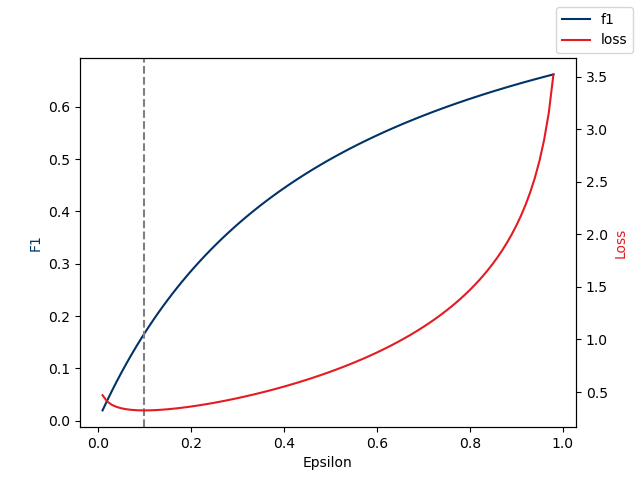
Figure 1: Loss vs $\text{F}_{1}\text{-Score}$

Or, to express the results more clearly, as the number of minority samples approaches 0, the $F_{1}\text{-Score}$ of the trivial solution approaches 0 (21), which compares rather poorly to the 0.5 achieved by random guessing.

$$\lim_{|\mathcal{B}_{\text{\tiny minority}}|\to 0}\;\frac{|\mathcal{B}_{\text{\tiny minority}}|}{0.5*|\mathcal{B}|+|\mathcal{B}_{\text{\tiny minority}}|}=0$$ (21)

The ”de-facto” solution to this problem is to generate new data points in the vicinity of other data points with the same class. This will alleviate the problem to an extend, since the best trivial solution will be equal to random guessing ($\frac{|\mathcal{B}_{\text{\tiny minority}}|}{|\mathcal{B|}}=0.5$). However, it does not guarantee that the loss (both test and train) is strictly inversely correlated to our discrete measure of success. Hence, we would like to generate new data ($\breve{\gamma}\in\mathcal{Y}$) such that minimizing $\mathcal{L}_{\mathcal{A}\cup\mathcal{Y}}$ will maximize $F_{1}\text{-Score}_{\mathcal{A}}$ and, if (12) is low, $F_{1}\text{-Score}_{\mathcal{B}}$.

In other words, we want to generate $\mathcal{Y}$ such that $\mathcal{L}_{\mathcal{A}\cup\mathcal{Y}}$ is inversely correlated to $F_{1}\text{-Score}_{\mathcal{A}}$. We will refer to any discrepancies of the $\mathcal{L}_{\mathcal{A}}$ and $F_{1}\text{-Score}_{\mathcal{A}}$ as the Performance-Error (22). Furthermore, we expand the Generalization error (12) to include the $F_{1}\text{-Score}$ (23) (or any other discrete measure of success).

$$\text{Performance-Error}_{\mathcal{A}}=1+\frac{\text{Cov}(F_{1}\text{-Score}_{\mathcal{A}},\mathcal{L}_{\mathcal{A}})}{\sqrt{\text{Var}(F_{1}\text{-Score}_{\mathcal{A}})\text{Var}(\mathcal{L}_{\mathcal{A}})}}$$ (22)

where $\mathcal{A}$ is interchangeable with $\mathcal{B}$.

$$\mathcal{E}_{F_{1}\text{-Score}}=F_{1}\text{-Score}_{\mathcal{B}}-F_{1}\text{-Score}_{\mathcal{A}}$$ (23)

Thus, the overall objective is to minimize (24). In our approach, we simplify this by designing the algorithm to optimize for a high $F_{1}\text{-Score}$. Hence, reducing (24) to (23).

$$\text{Total-Error}=\text{Performance-Error}_{\mathcal{A}}+\mathcal{E}$$ (24)

However, because of the discrete nature of the $F_{1}\text{-Score}$ it can not directly be used as a loss function for a data generation algorithm.

We solved this problem by training a GAN, using the Discriminator to estimate the $F_{1}\text{-Score}_{\mathcal{A}}(\theta_{\mathcal{Y}})$ (where $\theta_{\mathcal{Y}}$ are the parameters of a classification model that was trained on $\mathcal{Y}$), and the Generator to map random noise to $\mathcal{Y}$.

More formally, the Generator maps a random noise vector, denoted as $\kappa$, to a batch of training samples, denoted as $\mathcal{Y}$. We will denote a set of batches of generated data as $\mathbfcal{Y}$ which means $\breve{\gamma}\in\mathcal{Y}\in\mathbfcal{Y}$. Hence, the loss functions for the Discriminator (in our work referred to as Critic) and Generator, are (25) and (26) respectively.

$$\mathcal{L}_{\mathcal{A}}(\theta_{\text{\tiny dis}})$$ (25)

$$\equiv\sum_{\kappa\in\mathcal{K}}\mathcal{L}(z_{\text{\tiny dis}}(z_{\text{\tiny gen}}(\kappa;\theta_{\text{\tiny gen}});\theta_{\text{\tiny dis}}),F_{1}\text{-Score}(y_{\mathcal{A}},\theta_{z_{\text{\tiny gen}}(\kappa;\theta_{\text{\tiny gen}})}))$$

$$\equiv\sum_{\mathcal{Y}\in\mathbfcal{Y}}\mathcal{L}(z_{\text{\tiny dis}}(\mathcal{Y};\theta_{\text{\tiny dis}}),F_{1}\text{-Score}(y_{\mathcal{A}},\theta_{\mathcal{Y}}))$$

$$\mathcal{L}_{\mathcal{A}}(\theta_{\text{\tiny gen}})$$ (26)

$$\equiv\sum_{\kappa\in\mathcal{K}}\mathcal{L}(z_{\text{\tiny gen}}(\kappa;\theta_{\text{\tiny gen}}),z_{\text{\tiny dis}}(z_{\text{\tiny gen}}(\kappa;\theta_{\text{\tiny gen}});\theta_{\text{\tiny dis}}))$$

$$\equiv\sum_{\mathcal{Y}\in\mathbfcal{Y}}\mathcal{L}(\mathcal{Y},z_{\text{\tiny dis}}(\mathcal{Y};\theta_{\text{\tiny dis}}))$$

In the following three subsections we offer a more intuitive understanding of draGAN.

Model Overview

Similar to the vanilla GAN architecture, the Generator, a Neural Network, creates new data points by accepting a Gaussian noise vector as input. In our case, the data points generated correspond to a batch of training samples. This generated data is then used to train the classification model (i.e. a Logistic Regression model). Said model is subsequently evaluated on the actual training data. The metric for evaluation can be chosen liberally, which we demonstrate by using a discrete AUC score. The achieved performance is mapped to the generated training data used and then utilized as an X,y pair to train the Critic. In other words, the Critic will, over time, learn how valuable, from a classification performance perspective, each generated data point will be, which allows it to provide a meaningful loss to the Generator. This comes with the fortunate side product that one can train the model on discrete metrics, which the Critic will turn into a continuous loss for the Generator.

This architecture directly addresses the aforementioned problem of not taking the classification value of the generated data points into consideration. However, as a vigilant reader will have noticed, draGAN does not optimize either network to generate realistic data points. Even though this might intuitively seem like a problem, as the network could conceivably generate data that skews the classification model into an unrealistic direction, we empirically show that it results in better classification performances of the model, which is the overall objective of this architecture.

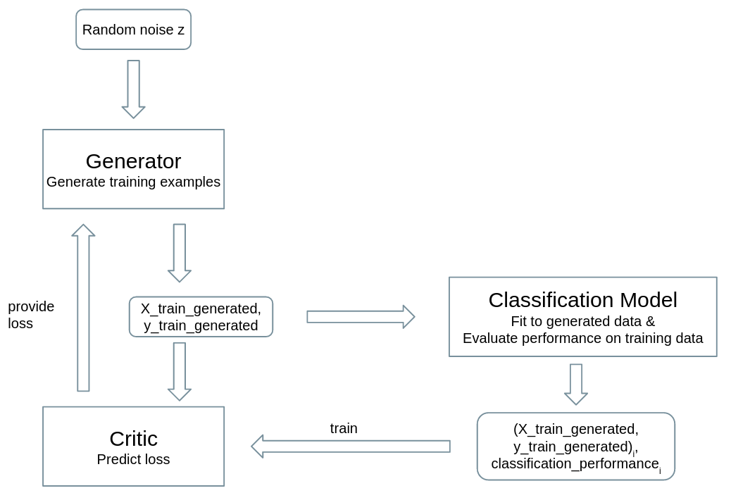
Figure 2: draGAN Architecture.

3.1 Generator

In Vanilla GAN, the Generator is used to map a random Gaussian noise vector to a sample that is hard to distinguish from the real data. However, since the network itself generates a single data point at a time, it oftentimes results in the Generator learning to map any random input to one, highly valued, data point [31]. When using a batch of generated samples to train the classification model, this poses an obvious problem.

Furthermore, even if the Generator does not collapse during training, the generated batch of data points might not be coherent. This means that the data points might be different from one another, and individually look realistic, but are not well distributed in the sample space. Therefore, a classification model trained on these generated data points will likely not perform well. The Generator used in draGAN solves this issue by using a 1-dimensional convolutional layer to generate batches of samples at every forward pass. It follows that the loss will not be provided for any one single sample, but for the whole batch. This intuitively makes sense as one will ultimately use a batch of generated samples to train the classifier and not individual samples.

3.2 Adversarial

In vanilla GAN the adversarial, referred to as Discriminator, learns to classify whether a provided sample originated from the real data or was generated by the Generator. This process was further improved by the Wasserstein GAN where the adversarial, referred to as Critic, estimates the Wasserstein-1 function for generated values. I.e. how much “earth” would have to be moved from the distribution curve of the generated sample, to convert it to a real sample. Both of these approaches work well for generating realistic data points. However, that is not the objective when using GAN based approaches to improve classification performance, as realistic samples do not necessarily correspond to high classification performance.

The adversarial in draGAN, referred to as Critic, addresses this problem by learning how to estimate the score, in our case AUC, that the classification model would achieve if it were trained on the generated data and assessed on the original training data. More concretely, the Critic learns to estimate the value of each generated batch with respect to the classifier’s performance on a chosen metric. Therefore, throughout training, samples generated by the Generator will be increasingly helpful to the classifier in learning the distribution of the real training data, ultimately resulting in a better performance. Furthermore, since the Critic will always provide a continuous loss to the Generator, even when trained on discrete values, draGAN can be trained to optimize the classifier’s performance on any metric, including AUC. This means that a classifier such as Logistic Regression can indirectly be optimized for any (discrete) metric. It is worth pointing out that similar to the Wasserstein GAN, draGAN has a mechanism for indicating convergence. Whilst the former uses the Wasserstein-1 function to measure the “distance” between generated and real samples, which gives a clear indication of whether the model is improving, the latter uses the Classification Models performance metric (i.e. AUC score) to indicate the same.

3.3 Training Process

The training process of draGAN is typical for most GAN based architectures, where both the Generator and Adversarial are re-trained frequently and the Adversarial is used to provide some loss to the Generator. The key difference is that usually, the Adversarial learns to classify samples to be either generated or real [10] or learns to estimate the similarity of a given sample to the real data [23]. In draGAN, however, the value of each generated sample is determined by training the classification model on the generated data and assessing its performance on the training data. Subsequently, these data points are used to train the Critic. This process draws similarities to Reinforcement learning. For example, similarly to the memory recall method proposed in [32], after each iteration, some of the Critic’s training data is saved for recalling in future training. [23] proposed to train the Critic until convergence in each iteration, because of the differentiability of Wasserstein-1, whilst [10] determined a single training step to be the optimum. Because of the non-differentiability of the function that the Critic in draGAN attempts to estimate, we do not train the Critic until convergence but empirically estimated a good value to be in the range from 10 to 100 steps. This, however, is a hyperparameter and thus the optimum will be subject to the size of the network and the data used.

4 Experimental Setup

To empirically evaluate the performance of draGAN, we benchmarked it on 94 imbalanced classification datasets (Table LABEL:datasets-table, in Appendix 6.1) against a plethora of state-of-the-art data generation algorithms from the SMOTE and GAN families. For these experiments we chose AUC to be the metric that draGAN is supposed to maximize.

4.1 Preprocessing

[14] is, to the best of our knowledge, the the most extensive empirical study of oversampling techniques. For ease of comparison between their work and ours, we utilize the exact same reprocessing and sampling pipeline.

4.2 Datasets

$N_{+}$ denotes the number minority class samples and $N_{-}$ the number of majority class samples (note $N=N_{+}+N_{-}$) and IR indicates the imbalance ratio (27).

$$\text{IR}=\frac{N_{-}}{N_{+}}$$ (27)

As proposed by [11] we use the difference of AUC scores achieved by a Random Forest Classifier and a Logistic Regression as an estimator of the linearity of each dataset. If the difference is greater than 0.1, the dataset is considered non-Linear.
An exhaustive table of all datasets used can in be found in Appendix 6.1

4.3 Performance Measure

As already pointed out, the accuracy of a classification model on an imbalanced dataset gives a very poor indication of performance. Therefore, we use three alternative measures that are commonly utilized to evaluate performances for imbalanced classification tasks [14, 33, 34, 35]. The notation is as follows, TP, TN, FP and FN correspond to true positive, true negative, false positive and false negative respectively.

G-score: which is sometimes referred to as Geometric Mean or G-Mean measures the balance between classification performances on both the majority and the minority classes.

$$G=\sqrt{\frac{\text{TP}}{\text{P}}*\frac{\text{TN}}{\text{N}}}$$ (28)

Where P$=$TP$+$FN and N$=$TN$+$FP

$\text{F}_{1}$-score: (which is a specific form of the F-score) is the harmonic mean of precision (29) and recall (30).

$$\text{Precision}=\frac{\text{TP}}{\text{TP}+\text{FP}}$$ (29)

$$\text{Recall}=\frac{\text{TP}}{\text{TP}+\text{FN}}$$ (30)

$$\text{F}_{1}=2*\frac{\text{Precision}*\text{Recall}}{\text{Precision}+\text{Recall}}$$ (31)

AUC-Score: which abbreviates Area Under the receiver operating characteristic Curve quantifies the graph of sensitives plotted against corresponding false positive rates by calculating the area under the curve.

$$\text{TPR}=\frac{\text{TP}}{\text{TP}+\text{FN}}$$ (32)

$$\text{FPR}=\frac{\text{FP}}{\text{FP}+\text{TN}}$$ (33)

$$\text{AUC}=\int_{0}^{1}{\text{TPR}(\text{FPR}^{-1}(x))dx}$$ (34)

4.4 Data-split

Classification performance is evaluated by repeated stratified k-fold cross-validation with 5 splits and 3 repeats.

4.5 Hyperparameter tuning

For Hyperparameter tuning of draGAN, 15 datasets were randomly selected. Each datataset was stratified with 5 splits, omitting the test data and using a fraction of the training data as validation, so that we do not skew the empirical results. Parameters were sampled via the Tree-structured Parzen Estimator algorithm, as implemented in Optuna. A list of all hyperparameters can be found in the Appendix 6.2.

5 Results

In this section we will analyze the performances of our benchmarks as compared to draGAN using the AUC-score. Because of it’s slow speed the cWGAN algorithm was only evaluated on a subset of the datasets. The cWGAN benchmarking and the results as evaluated on the other discrete measures of success can be found in the Appendix 6.4 and Appendix 6.5 respectively.
For ease of comparison, an ”Average” row was added to Table LABEL:table:results.

Table 1: Results

Nr	Dataset	Vanilla	SMOTE	Polynom_fit_SMOTE	MixUp	draGAN (ours)
0	cm1	0.729	0.7292	0.7292	0.7292	0.738
1	german	0.5537	0.5537	0.5537	0.5537	0.661
2	hepatitis	0.742	0.7428	0.7788	0.7639	0.783
3	hypothyroid	0.8111	0.8445	0.8483	0.826	0.8278
4	kc1	0.7962	0.7962	0.7962	0.7962	0.7972
5	pc1	0.657	0.657	0.657	0.657	0.7122
6	satimage	0.7027	0.7057	0.7153	0.7008	0.6902
7	spectf	0.8522	0.8501	0.8509	0.8522	0.8116
8	abalone_17_vs_7_8_9_10	0.7512	0.8436	0.8486	0.7626	0.9304
9	abalone_19_vs_10_11_12_13	0.454	0.7277	0.7255	0.5064	0.8063
10	abalone_20_vs_8_9_10	0.7548	0.9094	0.9167	0.7703	0.9747
11	abalone_21_vs_8	0.8957	0.9139	0.9157	0.9014	0.966
12	abalone_3_vs_11	1	1	1	1	0.9995
13	abalone9_18	0.731	0.7801	0.7955	0.7401	0.938
14	car_good	0.6223	0.6127	0.6205	0.6166	0.5922
15	car_vgood	0.9308	0.9335	0.9343	0.9296	0.9252
16	cleveland_0_vs_4	0.6097	0.6536	0.6435	0.6259	0.6958
17	ecoli_0_1_3_7_vs_2_6	0.9066	0.9189	0.9304	0.8823	0.9458
18	ecoli_0_1_4_6_vs_5	0.949	0.9429	0.9298	0.9449	0.9013
19	ecoli_0_1_4_7_vs_2_3_5_6	0.8461	0.8444	0.8351	0.8526	0.8304
20	ecoli_0_1_4_7_vs_5_6	0.8914	0.887	0.875	0.8982	0.8556
21	ecoli_0_1_vs_2_3_5	0.9198	0.9062	0.9143	0.9143	0.8695
22	ecoli_0_1_vs_5	0.9716	0.9652	0.958	0.9716	0.9121
23	ecoli_0_2_3_4_vs_5	0.9408	0.9232	0.9231	0.9358	0.8617
24	ecoli_0_2_6_7_vs_3_5	0.8645	0.8434	0.8537	0.861	0.7828
25	ecoli_0_3_4_6_vs_5	0.9419	0.9311	0.9203	0.9311	0.8703
26	ecoli_0_3_4_7_vs_5_6	0.8636	0.8621	0.8532	0.85	0.8538
27	ecoli_0_3_4_vs_5	0.9306	0.9111	0.9056	0.925	0.8361
28	ecoli_0_4_6_vs_5	0.9409	0.9226	0.9148	0.9345	0.8572
29	ecoli_0_6_7_vs_3_5	0.8792	0.8568	0.8622	0.8767	0.8406
30	ecoli_0_6_7_vs_5	0.9425	0.9342	0.9313	0.9363	0.8937
31	flaref	0.8854	0.9095	0.9117	0.8952	0.9012
32	glass_0_1_4_6_vs_2	0.6351	0.6058	0.6351	0.6314	0.6645
33	glass_0_1_5_vs_2	0.6344	0.5685	0.636	0.6185	0.6167
34	glass_0_1_6_vs_2	0.6238	0.5868	0.631	0.5978	0.6452
35	glass_0_1_6_vs_5	0.86	0.8762	0.86	0.8848	0.94
36	glass_0_4_vs_5	0.9625	0.9625	0.9625	0.9625	0.8668
37	glass_0_6_vs_5	0.8379	0.8642	0.8379	0.8262	0.9711
38	glass_0_1_2_3_vs_4_5_6	0.9763	0.9758	0.9769	0.9756	0.9714
39	glass0	0.7306	0.7396	0.7345	0.7286	0.8339
40	glass1	0.5245	0.5526	0.525	0.5368	0.5436
41	glass6	0.971	0.9713	0.971	0.9707	0.9569
42	glass2	0.657	0.6228	0.6553	0.6515	0.7172
43	glass4	0.765	0.7847	0.765	0.7719	0.8308
44	glass5	0.8732	0.8878	0.8683	0.8967	0.9569
45	kddcup_buffer_overflow_vs_back	1	1	1	1	1
46	kddcup_guess_passwd_vs_satan	0.9994	0.9994	0.9994	0.9994	0.9957
47	kddcup_land_vs_portsweep	0.999	0.999	0.999	0.999	0.998
48	kddcup_land_vs_satan	0.9994	0.9995	0.9995	0.9994	0.9997
49	kr_vs_k_one_vs_fifteen	1	1	1	1	1
50	kr_vs_k_three_vs_eleven1	0.9993	0.9996	0.9997	0.9994	0.9999
51	kr_vs_k_zero_one_vs_draw	0.9908	0.9881	0.9909	0.9908	0.9921
52	kr_vs_k_zero_vs_eight	0.9066	0.9243	0.9263	0.9067	0.9239
53	kr_vs_k_zero_vs_fifteen	0.999	1	1	0.9998	0.9995
54	led7digit_0_2_4_5_6_7_8_9_vs_1	0.914	0.9145	0.9109	0.9162	0.8916
55	lymphography_normal_fibrosis	0.9324	0.9929	0.9929	0.9369	0.8893
56	page_blocks_1_3_vs_4	0.9381	0.9389	0.9385	0.9385	0.95
57	poker_8_9_vs_51	0.561	0.4873	0.5306	0.5675	0.5196
58	poker_8_9_vs_6	0.4495	0.4421	0.4114	0.4336	0.3993
59	poker_8_vs_6	0.289	0.2863	0.2385	0.268	0.3229
60	poker_9_vs_7	0.6427	0.5755	0.5439	0.6085	0.5607
61	shuttle_2_vs_5	0.9928	0.9932	0.9927	0.9916	0.9966
62	shuttle_6_vs_2_3	1	1	1	1	0.9977
63	shuttle_c0_vs_c4	0.9879	0.9899	0.9891	0.9881	0.9999
64	shuttle_c2_vs_c4	0.975	0.9806	0.975	0.9736	0.9737
65	vowel0	0.9625	0.9633	0.9641	0.963	0.9549
66	winequality_red_3_vs_5	0.7944	0.792	0.7915	0.7947	0.71
67	winequality_red_4	0.6089	0.6126	0.6162	0.6096	0.6764
68	winequality_red_8_vs_6	0.6357	0.6489	0.6552	0.6381	0.8228
69	winequality_red_8_vs_6_7	0.6007	0.607	0.6138	0.6013	0.7653
70	winequality_white_3_9_vs_5	0.3703	0.3474	0.3404	0.4096	0.6509
71	winequality_white_3_vs_7	0.6185	0.5724	0.6165	0.6185	0.5269
72	winequality_white_9_vs_4	0.6367	0.709	0.7114	0.6256	0.8502
73	yeast_0_2_5_6_vs_3_7_8_9	0.8358	0.8208	0.8327	0.838	0.7835
74	yeast_0_2_5_7_9_vs_3_6_8	0.8877	0.8848	0.8858	0.8842	0.8327
75	yeast_0_3_5_9_vs_7_8	0.7468	0.7288	0.751	0.7373	0.7122
76	yeast_0_5_6_7_9_vs_4	0.8307	0.8392	0.8309	0.8312	0.8211
77	yeast_1_2_8_9_vs_7	0.7508	0.7813	0.7838	0.7524	0.79
78	yeast_1_4_5_8_vs_7	0.6827	0.6784	0.6758	0.6881	0.6343
79	yeast_1_vs_7	0.8136	0.8463	0.8442	0.8299	0.8429
80	yeast_2_vs_4	0.9161	0.9333	0.9286	0.9196	0.9312
81	yeast_2_vs_8	0.844	0.8349	0.8423	0.8505	0.7751
82	yeast4	0.8709	0.8814	0.8811	0.8745	0.8909
83	yeast5	0.9861	0.9861	0.9864	0.9861	0.9874
84	yeast6	0.9249	0.9299	0.9359	0.9279	0.927
85	yeast1	0.7803	0.7808	0.7834	0.7828	0.7749
86	yeast3	0.9629	0.9653	0.9654	0.9644	0.9336
87	zoo_3	0.7837	0.8272	0.8026	0.7895	0.7695
88	iris0	1	1	1	1	1
89	new_thyroid1	0.8857	0.8976	0.8992	0.8915	0.996
90	pima	0.7489	0.7621	0.774	0.7551	0.8088
91	segment0	0.8474	0.8611	0.8647	0.8538	0.964
92	vehicle0	0.8194	0.8231	0.8259	0.8219	0.9648
93	wisconsin	0.995	0.9951	0.9948	0.995	0.9939
	Average	0.8195	0.8259	0.827	0.8207	0.8391

As can be observed in Table LABEL:table:results, draGAN achieved the highest AUC score most frequently (42 times) followed by Vanilla (25 times), polynom_fit_SMOTE (22 times), MixUp (19 times) and SMOTE (18 times). Beyond simple ranking, draGAN achieved the overall highest average AUC score and a more than 2.6 times higher performance gain over the baseline (Vanilla) than the current state-of-the-art (polynom_fit_SMOTE).

5.1 Correlation of results

To gain a better understanding of how similar certain algorithms perform, we calculated the Pearson Correlation Coefficient w.r.t. vanilla logistic regression (35) for each one.

$$r_{i}=\frac{\sum_{k}(x_{i,k}-\bar{x}_{i})(y_{k}-\bar{y})}{\sqrt{\sum_{k}(x_{i,k}-\bar{x}_{i})^{2}\sum_{k}(y_{k}-\bar{y})^{2}}}$$ (35)

where $x_{i,k}$ denotes the performance achieved by algorithm i on dataset k, and $y_{k}$ the performance achieved by the vanilla logistic regression on dataset k.

What is interesting is that the performances of SMOTE, polynom_fit_SMOTE and MixUp are all highly correlated to the performance of the vanilla Logistic Regression (0.97, 0.97 and 0.99 respectively), whilst draGAN performs more independently (0.86).

5.2 Highest Performance gains over Vanilla Logistic Regression

To determine whether it is worth running draGAN in practise, we compare the individual top 10 percentage point performance gains of each algorithm over vanilla Logistic Regression.

SMOTE	polynom_fit_SMOTE	MixUp	draGAN (ours)
0.2737	0.2715	0.0524	0.3523
0.1546	0.1619	0.0393	0.2806
0.0924	0.0974	0.0248	0.2199
0.0723	0.0747	0.0235	0.2135
0.0605	0.0645	0.0219	0.207
0.0491	0.0605	0.0163	0.1871
0.0439	0.0372	0.0162	0.1792
0.0435	0.0368	0.0155	0.1646
0.0334	0.0338	0.0149	0.1454
0.0327	0.033	0.0123	0.1332
0.0856	0.0871	0.0237	0.2083

Table 2: Individual Top 10 percentage point gains over Vanilla Logistic Regression; the last line represents the averages of the above figures

As can be observed in Table 2, draGAN has both the single highest percentage point performance gain, and the highest average percentage point gain (out of the individual top 10 performances).
As a vigilant reader will have realized, the only way such a substantial performance gain and yet only a comparatively marginal overall average performance gain is possible, is when the algorithm under-performs the baseline on other datasets. Further research is required to figure out what exactly causes the algorithm to over/under perform and potentially stabilize it. However, as of now, it seems advisable for practitioners to train both draGAN and a more stable SMOTE variant, before choosing the final sampling method to be used.

As shown in the Appendix 6.4, draGAN, converges much faster than other GAN based methods and has fewer tune-able parameters. Hence, the overall temporal and computational cost associated with adding the algorithm to ones toolkit, is marginal, whilst the potential performance gain can be substantial.

5.3 Classification Performance as a function of available datapoints

Lastly, we investigate the performance drop-off experienced by the various classifiers with respect to the number of samples available. Figure 3 visualizes the relationship of the classifiers performances with respect to the fraction of the dataset, abalone_17_vs_7_8_9_10, used. The numbers given in the legend are the slopes of the best fit line for each classifier. draGAN has, by far, the smallest absolute slope, which indicates that it experiences the smallest drop-off in performance when only very limited data is available. This is likely because it makes use of all available data, not just the minority class, and is able extrapolate.

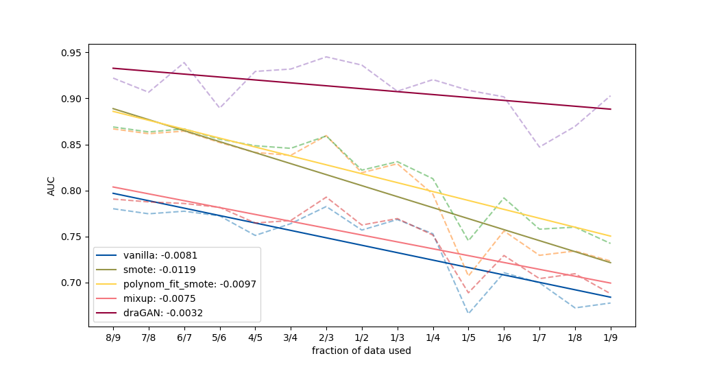
Figure 3: AUC score with varying data size

6 Conclusion

Even though we have successfully shown that our novel, task-oriented, data generation method, coined draGAN, is able to outperform the current state-of-the-art for generating new data points that improve the classification accuracy of a secondary model, we want to highlight the significant difference in approach to other GAN based models, rather than just the performance. To the best of our knowledge, this was the first time the adversarial was used to estimate the value of a generated data point in a domain beyond judging its realisticity. Since this approach is not limited to the aforementioned problem nor to any specific data type we hope to see its applications in different works in the future.

Authors’ contributions

• Leon Guertler: Ideation, conceptualization, implementation; Mathematical justifications; first draft

• Andri Ashfahani: Feedback & suggestions

• Anh Tuan Luu: Academic Supervision

Appendix

6.1 Datasets

Table 3: Datasets

	Dataset	N	#Features	IR	non-Linear
0	cm1	498	23	9.16	0
1	german	1000	29	2.33	0
2	hepatitis	155	19	3.84	0
3	hypothyroid	3163	25	19.95	1
4	kc1	2109	21	5.47	0
5	pc1	1109	21	13.40	0
6	satimage	6435	36	9.28	1
7	spectf	267	44	3.85	0
8	abalone_17_vs_7_8_9_10	2338	8	39.31	0
9	abalone_19_vs_10_11_12_13	1622	8	49.69	0
10	abalone_20_vs_8_9_10	1916	8	72.69	0
11	abalone_21_vs_8	581	8	40.5	1
12	abalone_3_vs_11	502	8	32.47	1
13	abalone9_18	731	8	16.40	0
14	car_good	1728	6	24.04	1
15	car_vgood	1728	6	25.58	1
16	cleveland_0_vs_4	177	23	12.62	0
17	ecoli_0_1_3_7_vs_2_6	281	7	39.14	0
18	ecoli_0_1_4_6_vs_5	280	6	13.0	0
19	ecoli_0_1_4_7_vs_2_3_5_6	336	7	10.59	0
20	ecoli_0_1_4_7_vs_5_6	332	6	12.28	0
21	ecoli_0_1_vs_2_3_5	244	7	9.17	0
22	ecoli_0_1_vs_5	240	6	11.0	0
23	ecoli_0_2_3_4_vs_5	202	7	9.1	0
24	ecoli_0_2_6_7_vs_3_5	224	7	9.18	0
25	ecoli_0_3_4_6_vs_5	205	7	9.25	0
26	ecoli_0_3_4_7_vs_5_6	257	7	9.28	0
27	ecoli_0_3_4_vs_5	200	7	9.0	0
28	ecoli_0_4_6_vs_5	203	6	9.15	0
29	ecoli_0_6_7_vs_3_5	222	7	9.09	0
30	ecoli_0_6_7_vs_5	220	6	10.0	0
31	flaref	1066	11	23.79	0
32	glass_0_1_4_6_vs_2	205	9	11.06	0
33	glass_0_1_5_vs_2	172	9	9.12	0
34	glass_0_1_6_vs_2	192	9	10.29	0
35	glass_0_1_6_vs_5	184	9	19.44	1
36	glass_0_4_vs_5	92	9	9.22	1
37	glass_0_6_vs_5	108	9	11.0	1
38	glass_0_1_2_3_vs_4_5_6	214	9	3.20	0
39	glass0	214	9	2.06	1
40	glass1	214	9	1.82	1
41	glass6	214	9	6.38	0
42	glass2	214	9	11.59	0
43	glass4	214	9	15.46	1
44	glass5	214	9	22.78	1
45	kddcup_buffer_overflow_vs_back	2233	31	73.43	0
46	kddcup_guess_passwd_vs_satan	1642	38	29.98	0
47	kddcup_land_vs_portsweep	1061	40	49.52	0
48	kddcup_land_vs_satan	1610	30	75.67	0
49	kr_vs_k_one_vs_fifteen	2244	6	27.77	0
50	kr_vs_k_three_vs_eleven1	2935	6	35.23	0
51	kr_vs_k_zero_one_vs_draw	2901	6	26.63	0
52	kr_vs_k_zero_vs_eight	1460	6	53.07	1
53	kr_vs_k_zero_vs_fifteen	2193	6	80.22	0
54	led7digit_0_2_4_5_6_7_8_9_vs_1	443	7	10.97	0
55	lymphography_normal_fibrosis	148	23	23.67	0
56	page_blocks_1_3_vs_4	472	10	15.86	0
57	poker_8_9_vs_51	2075	25	82.0	0
58	poker_8_9_vs_6	1485	25	58.4	0
59	poker_8_vs_6	1477	25	85.88	0
60	poker_9_vs_7	244	25	29.5	0
61	shuttle_2_vs_5	3316	9	66.67	0
62	shuttle_6_vs_2_3	230	9	22.0	0
63	shuttle_c0_vs_c4	1829	9	13.87	0
64	shuttle_c2_vs_c4	129	9	20.5	0
65	vowel0	988	13	9.978	0
66	winequality_red_3_vs_5	691	11	68.1	0
67	winequality_red_4	1599	11	29.17	0
68	winequality_red_8_vs_6	656	11	35.44	0
69	winequality_red_8_vs_6_7	855	11	46.5	0
70	winequality_white_3_9_vs_5	1482	11	58.28	0
71	winequality_white_3_vs_7	900	11	44.0	0
72	winequality_white_9_vs_4	168	11	32.6	1
73	yeast_0_2_5_6_vs_3_7_8_9	1004	10	9.14	1
74	yeast_0_2_5_7_9_vs_3_6_8	1004	10	9.14	1
75	yeast_0_3_5_9_vs_7_8	506	10	9.12	0
76	yeast_0_5_6_7_9_vs_4	528	10	9.35	1
77	yeast_1_2_8_9_vs_7	947	10	30.57	0
78	yeast_1_4_5_8_vs_7	693	10	22.1	0
79	yeast_1_vs_7	459	7	14.3	0
80	yeast_2_vs_4	514	8	9.08	1
81	yeast_2_vs_8	482	10	23.1	0
82	yeast4	1484	10	28.10	0
83	yeast5	1484	10	32.73	1
84	yeast6	1484	10	41.4	1
85	yeast1	1484	10	2.46	0
86	yeast3	1484	10	8.10	1
87	zoo_3	101	16	19.2	0
88	iris0	150	4	2.0	0
89	new_thyroid1	215	5	5.14	0
90	pima	768	8	1.87	0
91	segment0	2308	23	6.02	0
92	vehicle0	846	18	3.25	0
93	wisconsin	683	9	1.86	0

6.2 draGAN Hyperparameter tuning

Table LABEL:table:hyperparams-dragan shows the hyperparameters that performed best during the non-exhaustive Hyperparameter-tuning and were used for all experiments. All ambiguous hyperparameters are described in greater detail below the table.

Table 4: Hyperparameters (draGAN)

z_size	512
Generator Learning-Rate	0.000266
Generator Optimizer	RMSprop
Generator Activation	Sigmoid
Generator BatchNorm	No
Generator Dropout	Yes
Critic Learning-Rate	0.036284
Critic Nr. Epochs	2
Critic Optimizer	Adam
Critic Layer 1	64
Critic Layer 2	128
Critic Layer 3	64
Critic Activation 1	ReLU
Critic Activation 2	ReLU
Critic Activation 3	LeakyReLU
Critic BatchNorm Layer 1	Yes
Critic BatchNorm Layer 2	No
Critic Dropout Layer 1	No
Critic Dropout Layer 2	Yes
Nr. Samples Generated factor	1.793469
Total Epochs	1750
Batch Size	16
Max Memory Factor	124
Early Stopping	921

• Critic Nr. Epochs: Similarly to the training process of the original GAN architecture, the Critic is re-trained multiple times for each training step of the Generator.

• Nr. Samples Generated factor: This is the factor used to determine how many samples draGAN should generated, based on the number of training samples provided.

• Max Memory Factor: Similarly to the DQN architecture first proposed by [32], in each iteration, we retain some of the Critic’s training data for the next training iterations. The Max Memory Factor poses an upper limit to the number of samples in the models “memory”, which is enforced by deleting random elements thereof, rather than FIFO or FILO.

• Early Stopping: In draGAN, early stopping is evaluated based on for how many epochs the discrete measure of success (i.e. AUC) has not improved.

Figure 4 shows the exact architecture of the Generator and Critic in a diagrammatic form.

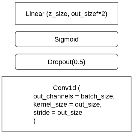
(a) Generator

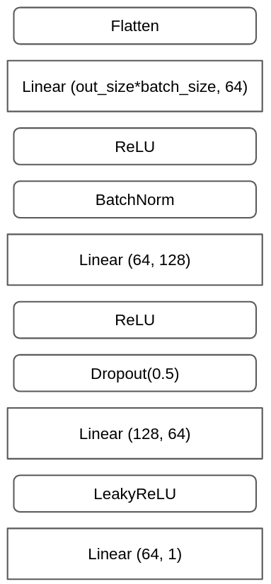
(b) Critic

Figure 4: draGAN Architecture

6.3 Experiment Hardware

For reproduction of our results, and specifically because we report the time take by each algorithm, below is a list of the hardware used for all experiments.

• AMD Threadripper 3970x

• NVIDIA GeForce RTX 3090

• RAM DDR4 3600 (128gb)

• Ubuntu 20.04

6.4 cWGAN results

As can be observed in Table LABEL:table:cWGAN-time, cWGAN, on average, takes more than 30-times as long to converge as draGAN. However, it is worthwhile pointing out that the library used, namely the one published by [11], runs on CPU whilst draGAN utilizes a GPU.

Table 5: Average Time (in seconds)

Nr	Dataset	Vanilla	SMOTE	Polynom_fit_SMOTE	MixUp	draGAN (ours)
cm1	0.0039	0.0057	0.006	0.0057	127.4778	528.7398
german	0.0045	0.0074	0.0063	0.008	194.2204	1070.6063
hepatitis	0.0046	0.0061	0.0052	0.0045	77.2097	160.3711
hypothyroid	0.0089	0.0178	0.0257	0.029	320.9317	9162.6501
kc1	0.0053	0.0083	0.0115	0.0125	235.6677	21622.0294
pc1	0.0043	0.0056	0.0088	0.0084	187.0925	1052.9057
satimage	0.0215	0.0526	0.0815	0.052	734.1355	32469.5402
spectf	0.0099	0.0078	0.013	0.0106	137.3585	357.6188
abalone_17_vs_7_8_9_10	0.0057	0.0086	0.0158	0.0143	244.8049	2056.5642
abalone_19_vs_10_11_12_13	0.0055	0.0071	0.0118	0.0109	170.4024	1448.2401
abalone_20_vs_8_9_10	0.0055	0.0079	0.0147	0.0119	183.5537	1594.7504
abalone_21_vs_8	0.0042	0.0055	0.0073	0.0064	98.9843	534.1806
abalone_3_vs_11	0.0042	0.0046	0.0069	0.0059	63.8179	473.0562
abalone9_18	0.0048	0.0061	0.0079	0.0073	87.9872	1160.8417
car_good	0.0047	0.0054	0.0096	0.0151	143.3904	6318.2594
car_vgood	0.0047	0.0067	0.0106	0.0152	140.254	22054.9514
Average	0.0064	0.0102	0.0152	0.0136	196.7055	6379.0816

Table LABEL:table:cWGAN_results shows the average AUC-Scores achieved by the different methods on the first 15 datasets. Even though draGAN seems to clearly outperform the rest (especially cWGAN), we want to emphasize that using merely 15 datasets is in no way statistically significant, and the results listed here are unlikely to generalize. This is why, cWGAN has been omitted from Table LABEL:table:results.

Table 6: AUC-Score

Dataset	Vanilla	SMOTE	Polynom_fit_SMOTE	MixUp	draGAN (ours)	cWGAN
cm1	0.729	0.7292	0.7292	0.7292	0.738	0.7291
german	0.5537	0.5537	0.5537	0.5537	0.661	0.5537
hepatitis	0.742	0.7428	0.7788	0.7639	0.783	0.7454
hypothyroid	0.8111	0.8445	0.8483	0.826	0.8278	0.832
kc1	0.7962	0.7962	0.7962	0.7962	0.7972	0.7964
pc1	0.657	0.657	0.657	0.657	0.7122	0.5082
satimage	0.7027	0.7057	0.7153	0.7008	0.6902	0.7127
spectf	0.8522	0.8501	0.8509	0.8522	0.8116	0.8458
abalone_17_vs_7_8_9_10	0.7512	0.8436	0.8486	0.7626	0.9304	0.6924
abalone_19_vs_10_11_12_13	0.454	0.7277	0.7255	0.5064	0.8063	0.4596
abalone_20_vs_8_9_10	0.7548	0.9094	0.9167	0.7703	0.9747	0.8454
abalone_21_vs_8	0.8957	0.9139	0.9157	0.9014	0.966	0.9116
abalone_3_vs_11	1	1	1	1	0.9995	1
abalone9_18	0.731	0.7801	0.7955	0.7401	0.938	0.7436
car_good	0.6223	0.6127	0.6205	0.6166	0.5922	0.4932
car_vgood	0.9308	0.9335	0.9343	0.9296	0.9252	0.8768
Average	0.7490	0.7875	0.7929	0.7566	0.8221	0.7341

6.5 Detailed results

Tables (LABEL:table:results_f1_score, LABEL:table:results_g1_score) show the performances achieved by the different benchmarking algorithms using a number of discrete measures of success. The decision boundary for each algorithm was determined using (36).

$$\text{Decision-Threshold}=\max_{\tiny\text{Threshold}}(\text{TPR}_{\tiny\text{Threshold}}-\text{FPR}_{\tiny\text{Threshold}})$$ (36)

where TPR is (32) and FPR (33)

Table 7: F1-Score

Nr	Dataset	Vanilla	SMOTE	Polynom_fit_SMOTE	MixUp	draGAN (ours)
0	cm1	0.3109	0.3109	0.3109	0.3109	0.3064
1	german	0.3926	0.3926	0.3926	0.3926	0.5058
2	hepatitis	0.461	0.4784	0.4995	0.4684	0.5168
3	hypothyroid	0.2183	0.2876	0.3086	0.2348	0.2434
4	kc1	0.4884	0.4884	0.4884	0.4884	0.4685
5	pc1	0.254	0.254	0.254	0.254	0.2621
6	satimage	0.3044	0.3056	0.3074	0.3071	0.2815
7	spectf	0.6083	0.6156	0.6107	0.6085	0.5601
8	abalone_17_vs_7_8_9_10	0.1362	0.2496	0.2334	0.1543	0.3314
9	abalone_19_vs_10_11_12_13	0.0412	0.1037	0.124	0.0492	0.1313
10	abalone_20_vs_8_9_10	0.0846	0.2288	0.194	0.0933	0.3356
11	abalone_21_vs_8	0.3026	0.3558	0.3558	0.3431	0.4585
12	abalone_3_vs_11	0.8	0.8	0.8	0.8	0.7911
13	abalone9_18	0.2685	0.2774	0.3107	0.263	0.447
14	car_good	0.103	0.1141	0.1086	0.1079	0.1081
15	car_vgood	0.3169	0.3368	0.3387	0.3144	0.3134
16	cleveland_0_vs_4	0.1694	0.1659	0.1824	0.1649	0.2147
17	ecoli_0_1_3_7_vs_2_6	0.0417	0.0536	0.0536	0.0369	0.0838
18	ecoli_0_1_4_6_vs_5	0.6148	0.6296	0.6348	0.6354	0.5965
19	ecoli_0_1_4_7_vs_2_3_5_6	0.4611	0.4676	0.4583	0.4905	0.4517
20	ecoli_0_1_4_7_vs_5_6	0.591	0.5822	0.5645	0.5638	0.5673
21	ecoli_0_1_vs_2_3_5	0.6532	0.5647	0.6011	0.5915	0.6152
22	ecoli_0_1_vs_5	0.6434	0.6512	0.6929	0.6306	0.6919
23	ecoli_0_2_3_4_vs_5	0.6435	0.6343	0.6651	0.6607	0.5903
24	ecoli_0_2_6_7_vs_3_5	0.5759	0.5487	0.5674	0.5776	0.5015
25	ecoli_0_3_4_6_vs_5	0.6762	0.6921	0.6762	0.673	0.629
26	ecoli_0_3_4_7_vs_5_6	0.5585	0.5545	0.5439	0.5416	0.5836
27	ecoli_0_3_4_vs_5	0.6268	0.6112	0.6317	0.6255	0.6101
28	ecoli_0_4_6_vs_5	0.6762	0.675	0.6619	0.6847	0.6133
29	ecoli_0_6_7_vs_3_5	0.5779	0.5917	0.5902	0.5854	0.553
30	ecoli_0_6_7_vs_5	0.6667	0.6556	0.6286	0.6318	0.5615
31	flaref	0.2632	0.3118	0.316	0.2794	0.3198
32	glass_0_1_4_6_vs_2	0.2617	0.2385	0.2661	0.2518	0.2459
33	glass_0_1_5_vs_2	0.218	0.2108	0.2154	0.2087	0.1941
34	glass_0_1_6_vs_2	0.1812	0.1681	0.1812	0.1641	0.2206
35	glass_0_1_6_vs_5	0.3778	0.3568	0.3778	0.3763	0.4422
36	glass_0_4_vs_5	0.4444	0.4444	0.4444	0.4444	0.3404
37	glass_0_6_vs_5	0.42	0.3844	0.42	0.4022	0.437
38	glass_0_1_2_3_vs_4_5_6	0.8628	0.871	0.8628	0.8592	0.8446
39	glass0	0.6665	0.6621	0.6665	0.6641	0.7169
40	glass1	0.3028	0.4119	0.3028	0.39	0.4996
41	glass6	0.8388	0.8247	0.8388	0.8388	0.7578
42	glass2	0.1899	0.1915	0.1899	0.1889	0.2363
43	glass4	0.4027	0.3971	0.4027	0.4071	0.4354
44	glass5	0.3205	0.3205	0.3205	0.3229	0.3631
45	kddcup_buffer_overflow_vs_back	0.9091	0.9091	0.9091	0.9091	0.9091
46	kddcup_guess_passwd_vs_satan	0.9417	0.9417	0.9417	0.9417	0.9036
47	kddcup_land_vs_portsweep	0.8421	0.8421	0.8421	0.8421	0.8135
48	kddcup_land_vs_satan	0.8254	0.8421	0.8421	0.8254	0.8492
49	kr_vs_k_one_vs_fifteen	0.9669	0.9669	0.9669	0.9669	0.9669
50	kr_vs_k_three_vs_eleven1	0.9136	0.9504	0.9447	0.9275	0.9604
51	kr_vs_k_zero_one_vs_draw	0.7631	0.6925	0.8007	0.8074	0.7263
52	kr_vs_k_zero_vs_eight	0.3773	0.3042	0.3053	0.3804	0.3382
53	kr_vs_k_zero_vs_fifteen	0.8012	0.897	0.897	0.8743	0.8691
54	led7digit_0_2_4_5_6_7_8_9_vs_1	0.5728	0.6948	0.6131	0.5674	0.5662
55	lymphography_normal_fibrosis	0.0667	0.1333	0.1333	0.0889	0.0822
56	page_blocks_1_3_vs_4	0.5245	0.5268	0.5268	0.5268	0.6998
57	poker_8_9_vs_51	0.0671	0.026	0.0418	0.0596	0.0497
58	poker_8_9_vs_6	0.0353	0.038	0.0305	0.035	0.0396
59	poker_8_vs_6	0.014	0.0159	0.0168	0.0169	0.0192
60	poker_9_vs_7	0.0489	0.0208	0.0174	0.0444	0.015
61	shuttle_2_vs_5	0.6984	0.7126	0.6984	0.6283	0.8097
62	shuttle_6_vs_2_3	0.6667	0.6667	0.6667	0.6667	0.6444
63	shuttle_c0_vs_c4	0.8588	0.9132	0.9006	0.8704	0.9766
64	shuttle_c2_vs_c4	0.0444	0.0714	0.0444	0.0658	0.0714
65	vowel0	0.8079	0.7839	0.8002	0.801	0.6253
66	winequality_red_3_vs_5	0.1155	0.1461	0.144	0.1102	0.0774
67	winequality_red_4	0.1232	0.1461	0.1479	0.1221	0.1328
68	winequality_red_8_vs_6	0.0955	0.1247	0.1461	0.0977	0.1412
69	winequality_red_8_vs_6_7	0.0389	0.0505	0.0595	0.0398	0.1024
70	winequality_white_3_9_vs_5	0.0753	0.0399	0.072	0.0949	0.087
71	winequality_white_3_vs_7	0.22	0.0759	0.2212	0.2158	0.1118
72	winequality_white_9_vs_4	0	0	0	0	0
73	yeast_0_2_5_6_vs_3_7_8_9	0.5494	0.5648	0.5572	0.5756	0.5399
74	yeast_0_2_5_7_9_vs_3_6_8	0.6839	0.6746	0.6864	0.6786	0.6513
75	yeast_0_3_5_9_vs_7_8	0.3924	0.3623	0.4012	0.3787	0.3827
76	yeast_0_5_6_7_9_vs_4	0.5198	0.514	0.4761	0.5267	0.4469
77	yeast_1_2_8_9_vs_7	0.1382	0.1573	0.1336	0.1479	0.161
78	yeast_1_4_5_8_vs_7	0.1616	0.1782	0.1613	0.168	0.1407
79	yeast_1_vs_7	0.2623	0.3165	0.3158	0.274	0.3465
80	yeast_2_vs_4	0.7065	0.7211	0.7226	0.7264	0.5624
81	yeast_2_vs_8	0.4671	0.4302	0.4744	0.4692	0.3353
82	yeast4	0.3358	0.2814	0.3435	0.3356	0.2916
83	yeast5	0.6107	0.6145	0.6028	0.6089	0.6144
84	yeast6	0.3851	0.3305	0.3314	0.3612	0.3186
85	yeast1	0.6038	0.6047	0.6107	0.6088	0.6024
86	yeast3	0.6531	0.6652	0.6632	0.6561	0.6355
87	zoo_3	0	0	0	0	0
88	iris0	0.9474	0.9474	0.9474	0.9474	0.9474
89	new_thyroid1	0.6757	0.7021	0.7028	0.6797	0.8839
90	pima	0.6176	0.633	0.6473	0.6223	0.6666
91	segment0	0.4825	0.5083	0.5075	0.4967	0.7591
92	vehicle0	0.5869	0.5908	0.5907	0.5897	0.821
93	wisconsin	0.963	0.9628	0.9611	0.9635	0.953
	Average	0.4487	0.4549	0.4592	0.4513	0.4641

Table 8: G-Score

Nr	Dataset	Vanilla	SMOTE	Polynom_fit_SMOTE	MixUp	draGAN (ours)
0	cm1	0.649	0.649	0.649	0.649	0.6823
1	german	0.5309	0.5309	0.5309	0.5309	0.6096
2	hepatitis	0.6586	0.6731	0.6849	0.6752	0.6847
3	hypothyroid	0.7477	0.811	0.8258	0.7703	0.7819
4	kc1	0.7276	0.7276	0.7276	0.7276	0.7255
5	pc1	0.5741	0.5741	0.5741	0.5741	0.6799
6	satimage	0.6789	0.6796	0.6801	0.6687	0.6512
7	spectf	0.7884	0.7845	0.7825	0.7911	0.745
8	abalone_17_vs_7_8_9_10	0.6838	0.7542	0.7597	0.6947	0.8562
9	abalone_19_vs_10_11_12_13	0.4094	0.6466	0.6119	0.4439	0.7265
10	abalone_20_vs_8_9_10	0.6349	0.7873	0.7958	0.643	0.8612
11	abalone_21_vs_8	0.7064	0.7207	0.7208	0.7127	0.7556
12	abalone_3_vs_11	0.8165	0.8165	0.8165	0.8165	0.8162
13	abalone9_18	0.6734	0.7032	0.7145	0.6606	0.8478
14	car_good	0.5454	0.6064	0.579	0.5754	0.5883
15	car_vgood	0.8758	0.8829	0.8827	0.8742	0.8687
16	cleveland_0_vs_4	0.4359	0.4181	0.4429	0.4529	0.4663
17	ecoli_0_1_3_7_vs_2_6	0.2361	0.2498	0.2498	0.2215	0.2601
18	ecoli_0_1_4_6_vs_5	0.8008	0.7905	0.7867	0.7989	0.7722
19	ecoli_0_1_4_7_vs_2_3_5_6	0.741	0.7499	0.7208	0.747	0.7375
20	ecoli_0_1_4_7_vs_5_6	0.7646	0.7649	0.7598	0.7693	0.7612
21	ecoli_0_1_vs_2_3_5	0.8048	0.7754	0.7866	0.7882	0.7678
22	ecoli_0_1_vs_5	0.8266	0.8154	0.8091	0.8252	0.7886
23	ecoli_0_2_3_4_vs_5	0.7959	0.7771	0.784	0.7922	0.7491
24	ecoli_0_2_6_7_vs_3_5	0.7412	0.7219	0.7356	0.7414	0.6922
25	ecoli_0_3_4_6_vs_5	0.7865	0.7875	0.7865	0.7858	0.7715
26	ecoli_0_3_4_7_vs_5_6	0.7692	0.7694	0.7672	0.7623	0.7635
27	ecoli_0_3_4_vs_5	0.7878	0.7686	0.7676	0.7868	0.728
28	ecoli_0_4_6_vs_5	0.786	0.782	0.7807	0.7865	0.7666
29	ecoli_0_6_7_vs_3_5	0.7553	0.7422	0.7513	0.757	0.7243
30	ecoli_0_6_7_vs_5	0.8105	0.8096	0.8038	0.8032	0.7553
31	flaref	0.8076	0.8302	0.8295	0.8203	0.8133
32	glass_0_1_4_6_vs_2	0.5591	0.5352	0.5608	0.5608	0.5438
33	glass_0_1_5_vs_2	0.5752	0.5599	0.5714	0.5559	0.5139
34	glass_0_1_6_vs_2	0.4916	0.4678	0.4916	0.4655	0.5713
35	glass_0_1_6_vs_5	0.5468	0.5403	0.5468	0.5461	0.5589
36	glass_0_4_vs_5	0.5361	0.5361	0.5361	0.5361	0.4507
37	glass_0_6_vs_5	0.4701	0.4372	0.4701	0.4537	0.5465
38	glass_0_1_2_3_vs_4_5_6	0.9054	0.9043	0.9054	0.9032	0.9047
39	glass0	0.693	0.7117	0.693	0.6976	0.7893
40	glass1	0.3529	0.4859	0.3529	0.4319	0.5199
41	glass6	0.8638	0.8651	0.8638	0.8638	0.861
42	glass2	0.5716	0.5532	0.5716	0.5639	0.6128
43	glass4	0.6496	0.6501	0.6496	0.6501	0.6677
44	glass5	0.5462	0.5462	0.5462	0.5468	0.5419
45	kddcup_buffer_overflow_vs_back	0.9129	0.9129	0.9129	0.9129	0.9129
46	kddcup_guess_passwd_vs_satan	0.9513	0.9513	0.9513	0.9513	0.9493
47	kddcup_land_vs_portsweep	0.8713	0.8713	0.8713	0.8713	0.8686
48	kddcup_land_vs_satan	0.8712	0.8714	0.8714	0.8712	0.8715
49	kr_vs_k_one_vs_fifteen	0.9674	0.9674	0.9674	0.9674	0.9674
50	kr_vs_k_three_vs_eleven1	0.9669	0.9681	0.9679	0.9674	0.9684
51	kr_vs_k_zero_one_vs_draw	0.9487	0.9482	0.9524	0.9528	0.9517
52	kr_vs_k_zero_vs_eight	0.82	0.8456	0.8431	0.8251	0.8414
53	kr_vs_k_zero_vs_fifteen	0.9004	0.9018	0.9018	0.9015	0.9013
54	led7digit_0_2_4_5_6_7_8_9_vs_1	0.7302	0.8183	0.721	0.7343	0.7184
55	lymphography_normal_fibrosis	0.1336	0.1414	0.1414	0.1371	0.1363
56	page_blocks_1_3_vs_4	0.8374	0.8385	0.8385	0.8385	0.8627
57	poker_8_9_vs_51	0.4602	0.3696	0.3968	0.4605	0.4188
58	poker_8_9_vs_6	0.3894	0.4065	0.3121	0.3671	0.3249
59	poker_8_vs_6	0.2266	0.2201	0.1994	0.2821	0.3313
60	poker_9_vs_7	0.3012	0.1142	0.1072	0.2751	0.0878
61	shuttle_2_vs_5	0.9426	0.9429	0.9426	0.9375	0.9414
62	shuttle_6_vs_2_3	0.7071	0.7071	0.7071	0.7071	0.7055
63	shuttle_c0_vs_c4	0.9654	0.9705	0.9694	0.9664	0.9793
64	shuttle_c2_vs_c4	0.1225	0.1265	0.1225	0.1204	0.1251
65	vowel0	0.9161	0.9128	0.915	0.9151	0.8893
66	winequality_red_3_vs_5	0.5795	0.5773	0.5762	0.4836	0.5329
67	winequality_red_4	0.5654	0.5584	0.5595	0.5645	0.6047
68	winequality_red_8_vs_6	0.5785	0.5893	0.5919	0.5783	0.6823
69	winequality_red_8_vs_6_7	0.3558	0.3465	0.3509	0.3572	0.6229
70	winequality_white_3_9_vs_5	0.1772	0.2109	0.1076	0.2187	0.5852
71	winequality_white_3_vs_7	0.4691	0.4363	0.4689	0.4682	0.3758
72	winequality_white_9_vs_4	0	0	0	0	0
73	yeast_0_2_5_6_vs_3_7_8_9	0.7825	0.7607	0.7812	0.7816	0.7462
74	yeast_0_2_5_7_9_vs_3_6_8	0.8358	0.8262	0.8346	0.8296	0.8053
75	yeast_0_3_5_9_vs_7_8	0.679	0.677	0.6865	0.6808	0.678
76	yeast_0_5_6_7_9_vs_4	0.778	0.7857	0.7789	0.7723	0.7609
77	yeast_1_2_8_9_vs_7	0.627	0.6626	0.6569	0.6285	0.6695
78	yeast_1_4_5_8_vs_7	0.6	0.5979	0.5917	0.6082	0.5714
79	yeast_1_vs_7	0.6633	0.7246	0.7119	0.6947	0.7263
80	yeast_2_vs_4	0.8516	0.862	0.8599	0.8516	0.8286
81	yeast_2_vs_8	0.6396	0.6456	0.6404	0.6481	0.6474
82	yeast4	0.8139	0.8087	0.816	0.8136	0.8132
83	yeast5	0.9251	0.9256	0.9252	0.9251	0.9246
84	yeast6	0.8281	0.8305	0.834	0.8333	0.8287
85	yeast1	0.7127	0.7144	0.7152	0.7175	0.7138
86	yeast3	0.9058	0.9106	0.9086	0.9063	0.8733
87	zoo_3	0	0	0	0	0
88	iris0	0.9487	0.9487	0.9487	0.9487	0.9487
89	new_thyroid1	0.7997	0.8198	0.8209	0.8104	0.9161
90	pima	0.6916	0.7066	0.7194	0.6931	0.7318
91	segment0	0.7878	0.8106	0.8052	0.7949	0.9208
92	vehicle0	0.7537	0.7587	0.7579	0.7576	0.9108
93	wisconsin	0.9739	0.9733	0.9728	0.9736	0.9669
	Average	0.6742	0.6805	0.6776	0.6758	0.696

References

-
[1]
S. Lessmann, B. Baesens, H.-V. Seow, L. C. Thomas,
Benchmarking
state-of-the-art classification algorithms for credit scoring: An update of
research, European Journal of Operational Research 247 (1) (2015) 124–136.
doi:https://doi.org/10.1016/j.ejor.2015.05.030.
URL https://www.sciencedirect.com/science/article/pii/S0377221715004208 - [2] Y. Kou, C.-T. Lu, S. Sirwongwattana, Y.-P. Huang, Survey of fraud detection techniques, in: IEEE International Conference on Networking, Sensing and Control, 2004, Vol. 2, 2004, pp. 749–754 Vol.2. doi:10.1109/ICNSC.2004.1297040.
- [3] A. Ali, S. M. H. Shamsuddin, A. L. Ralescu, Classification with class imbalance problem: A review, in: SOCO 2015, 2015.
-
[4]
Y. SUN, A. K. C. WONG, M. S. KAMEL,
Classification of imbalanced
data: A review, International Journal of Pattern Recognition and Artificial
Intelligence 23 (04) (2009) 687–719.
arXiv:https://doi.org/10.1142/S0218001409007326, doi:10.1142/S0218001409007326.
URL https://doi.org/10.1142/S0218001409007326 - [5] M. Galar, A. Fernandez, E. Barrenechea, H. Bustince, F. Herrera, A review on ensembles for the class imbalance problem: Bagging-, boosting-, and hybrid-based approaches, IEEE Transactions on Systems, Man, and Cybernetics, Part C (Applications and Reviews) 42 (4) (2012) 463–484. doi:10.1109/TSMCC.2011.2161285.
-
[6]
W. A. Rivera, P. Xanthopoulos,
A
priori synthetic over-sampling methods for increasing classification
sensitivity in imbalanced data sets, Expert Systems with Applications 66
(2016) 124–135.
doi:https://doi.org/10.1016/j.eswa.2016.09.010.
URL https://www.sciencedirect.com/science/article/pii/S0957417416304882 - [7] Y. C. Zhuoyuan Zheng, Y. Li, Oversampling method for imbalanced classification, Computing and Informatics 34 (5) (2015) 1017–1037.
-
[8]
B. A. Talpur, D. O’Sullivan,
Multi-class imbalance in text
classification: A feature engineering approach to detect cyberbullying in
twitter, Informatics 7 (4).
doi:10.3390/informatics7040052.
URL https://www.mdpi.com/2227-9709/7/4/52 - [9] N. V. Chawla, K. W. Bowyer, L. O. Hall, W. P. Kegelmeyer, Smote: Synthetic minority over-sampling technique, J. Artif. Int. Res. 16 (1) (2002) 321–357.
-
[10]
I. Goodfellow, J. Pouget-Abadie, M. Mirza, B. Xu, D. Warde-Farley, S. Ozair,
A. Courville, Y. Bengio,
Generative
adversarial nets, in: Z. Ghahramani, M. Welling, C. Cortes, N. Lawrence,
K. Weinberger (Eds.), Advances in Neural Information Processing Systems,
Vol. 27, Curran Associates, Inc., 2014.
URL https://proceedings.neurips.cc/paper/2014/file/5ca3e9b122f61f8f06494c97b1afccf3-Paper.pdf -
[11]
J. Engelmann, S. Lessmann,
Conditional
wasserstein gan-based oversampling of tabular data for imbalanced learning,
Expert Systems with Applications 174 (2021) 114582.
doi:https://doi.org/10.1016/j.eswa.2021.114582.
URL https://www.sciencedirect.com/science/article/pii/S0957417421000233 - [12] F. Last, G. Douzas, F. Bação, Oversampling for imbalanced learning based on k-means and smote.
-
[13]
J. Zhai, J. Qi, C. Shen,
Binary imbalanced data
classification based on diversity oversampling by generative models, Inf.
Sci. 585 (C) (2022) 313–343.
doi:10.1016/j.ins.2021.11.058.
URL https://doi.org/10.1016/j.ins.2021.11.058 -
[14]
G. Kovács,
An
empirical comparison and evaluation of minority oversampling techniques on a
large number of imbalanced datasets, Applied Soft Computing 83 (2019)
105662.
doi:https://doi.org/10.1016/j.asoc.2019.105662.
URL https://www.sciencedirect.com/science/article/pii/S1568494619304429 - [15] S. Gazzah, N. E. B. Amara, New oversampling approaches based on polynomial fitting for imbalanced data sets, in: 2008 The Eighth IAPR International Workshop on Document Analysis Systems, 2008, pp. 677–684. doi:10.1109/DAS.2008.74.
-
[16]
H. Zhang, M. Cisse, Y. N. Dauphin, D. Lopez-Paz,
mixup: Beyond empirical risk
minimization, in: International Conference on Learning Representations,
2018.
URL https://openreview.net/forum?id=r1Ddp1-Rb - [17] Y. Luo, B.-L. Lu, Eeg data augmentation for emotion recognition using a conditional wasserstein gan, in: 2018 40th Annual International Conference of the IEEE Engineering in Medicine and Biology Society (EMBC), 2018, pp. 2535–2538. doi:10.1109/EMBC.2018.8512865.
- [18] Y. Saito, S. Takamichi, H. Saruwatari, Text-to-speech synthesis using stft spectra based on low-/multi-resolution generative adversarial networks, in: 2018 IEEE International Conference on Acoustics, Speech and Signal Processing (ICASSP), 2018, pp. 5299–5303. doi:10.1109/ICASSP.2018.8461714.
- [19] T. Xu, P. Zhang, Q. Huang, H. Zhang, Z. Gan, X. Huang, X. He, Attngan: Fine-grained text to image generation with attentional generative adversarial networks, in: 2018 IEEE/CVF Conference on Computer Vision and Pattern Recognition, 2018, pp. 1316–1324. doi:10.1109/CVPR.2018.00143.
-
[20]
E. Brophy, Z. Wang, Q. She, T. Ward,
Generative adversarial networks in
time series: A survey and taxonomy, CoRR abs/2107.11098.
arXiv:2107.11098.
URL https://arxiv.org/abs/2107.11098 -
[21]
U. Fiore, A. De Santis, F. Perla, P. Zanetti, F. Palmieri,
Using
generative adversarial networks for improving classification effectiveness in
credit card fraud detection, Information Sciences 479 (2019) 448–455.
doi:https://doi.org/10.1016/j.ins.2017.12.030.
URL https://www.sciencedirect.com/science/article/pii/S0020025517311519 -
[22]
I. J. Goodfellow, NIPS 2016 tutorial:
Generative adversarial networks, CoRR abs/1701.00160.
arXiv:1701.00160.
URL http://arxiv.org/abs/1701.00160 -
[23]
M. Arjovsky, S. Chintala, L. Bottou,
Wasserstein gan (2017).
doi:10.48550/ARXIV.1701.07875.
URL https://arxiv.org/abs/1701.07875 -
[24]
I. Gulrajani, F. Ahmed, M. Arjovsky, V. Dumoulin, A. C. Courville,
Improved
training of wasserstein gans, in: I. Guyon, U. V. Luxburg, S. Bengio,
H. Wallach, R. Fergus, S. Vishwanathan, R. Garnett (Eds.), Advances in Neural
Information Processing Systems, Vol. 30, Curran Associates, Inc., 2017.
URL https://proceedings.neurips.cc/paper/2017/file/892c3b1c6dccd52936e27cbd0ff683d6-Paper.pdf -
[25]
M. Mirza, S. Osindero, Conditional
generative adversarial nets, CoRR abs/1411.1784.
arXiv:1411.1784.
URL http://arxiv.org/abs/1411.1784 -
[26]
A. Odena, C. Olah, J. Shlens,
Conditional image synthesis with
auxiliary classifier gans (2016).
doi:10.48550/ARXIV.1610.09585.
URL https://arxiv.org/abs/1610.09585 - [27] N. Kodali, J. Abernethy, J. Hays, Z. Kira, How to train your dragan, arXiv preprint arXiv:1705.07215 2 (4).
-
[28]
D. A. Roberts, S. Yaida, B. Hanin, The
principles of deep learning theory, CoRR abs/2106.10165.
arXiv:2106.10165.
URL https://arxiv.org/abs/2106.10165 -
[29]
D. C. Blair,
Information
retrieval, 2nd ed. c.j. van rijsbergen. london: Butterworths; 1979: 208 pp.
price: $32.50, Journal of the American Society for Information Science
30 (6) (1979) 374–375.
arXiv:https://asistdl.onlinelibrary.wiley.com/doi/pdf/10.1002/asi.4630300621,
doi:https://doi.org/10.1002/asi.4630300621.
URL https://asistdl.onlinelibrary.wiley.com/doi/abs/10.1002/asi.4630300621 - [30] P. Flach, J. Hernandez-Orallo, C. Ferri, A coherent interpretation of auc as a measure of aggregated classification performance., 2011, pp. 657–664.
-
[31]
L. Metz, B. Poole, D. Pfau, J. Sohl-Dickstein,
Unrolled generative adversarial
networks, CoRR abs/1611.02163.
arXiv:1611.02163.
URL http://arxiv.org/abs/1611.02163 -
[32]
V. Mnih, K. Kavukcuoglu, D. Silver, A. A. Rusu, J. Veness, M. G. Bellemare,
A. Graves, M. Riedmiller, A. K. Fidjeland, G. Ostrovski, S. Petersen,
C. Beattie, A. Sadik, I. Antonoglou, H. King, D. Kumaran, D. Wierstra,
S. Legg, D. Hassabis, Human-level
control through deep reinforcement learning, Nature 518 (7540) (2015)
529–533.
doi:10.1038/nature14236.
URL https://doi.org/10.1038/nature14236 - [33] T. Raeder, G. Forman, N. Chawla, Learning from imbalanced data: Evaluation matters, 2012.
-
[34]
V. López, A. Fernández, S. García, V. Palade, F. Herrera,
An
insight into classification with imbalanced data: Empirical results and
current trends on using data intrinsic characteristics, Information Sciences
250 (2013) 113–141.
doi:https://doi.org/10.1016/j.ins.2013.07.007.
URL https://www.sciencedirect.com/science/article/pii/S0020025513005124 -
[35]
V. López, A. Fernández, F. Herrera,
On
the importance of the validation technique for classification with imbalanced
datasets: Addressing covariate shift when data is skewed, Information
Sciences 257 (2014) 1–13.
doi:https://doi.org/10.1016/j.ins.2013.09.038.
URL https://www.sciencedirect.com/science/article/pii/S0020025513006804