Data-Adaptive Discriminative Feature Localization with Statistically Guaranteed Interpretation

Abstract

In explainable artificial intelligence, discriminative feature localization is critical to reveal a blackbox model’s decision-making process from raw data to prediction. In this article, we use two real datasets, the MNIST handwritten digits and MIT-BIH Electrocardiogram (ECG) signals, to motivate key characteristics of discriminative features, namely adaptiveness, predictive importance and effectiveness. Then, we develop a localization framework based on adversarial attacks to effectively localize discriminative features. In contrast to existing heuristic methods, we also provide a statistically guaranteed interpretability of the localized features by measuring a generalized partial $R^{2}$. We apply the proposed method to the MNIST dataset and the MIT-BIH dataset with a convolutional auto-encoder. In the first, the compact image regions localized by the proposed method are visually appealing. Similarly, in the second, the identified ECG features are biologically plausible and consistent with cardiac electrophysiological principles while locating subtle anomalies in a QRS complex that may not be discernible by the naked eye. Overall, the proposed method compares favorably with state-of-the-art competitors. Accompanying this paper is a Python library dnn-locate that implements the proposed approach.

Institute of Mathematical Statistics

, , , and

1 Introduction

The empirical success of machine learning in real applications has profound impacts on many scientific and engineering areas, including image analysis (LeCun et al., 1989; He et al., 2016), recommender systems (Wang, Wang and Yeung, 2015), natural language processing (Hochreiter and Schmidhuber, 1997), drug discovery (Vamathevan et al., 2019), protein structure prediction (Jumper et al., 2021; Evans et al., 2021). However, the nature of a black-box model makes it challenging to interpret its decision-making process. The lack of interpretability hinders transparency, trust, and understanding of scientific discovery. To meet challenges, Explainable AI (XAI) is emerging, which includes localizing discriminative features attributing to a model’s predictive performance, shaping or confirming human intuitions and knowledge, for instance, visual explanation on image recognition.

1.1 Motivation: DL discriminative localization in the MIT-BIH ECG dataset

Our investigation responds to the need for locating features that are most critical to a learning outcome. The present study is motivated by the MIT-BIH ECG dataset and the MNIST dataset. Specifically, the MNIST dataset serves as a benchmark for studying XAI methods (Ribeiro, Singh and Guestrin, 2016; Lundberg and Lee, 2017), in part because the results of Localization could be easily evaluated by human intuition. As demonstrated in Figures 3 and 7, localized image pixels explain how a deep convolutional network differentiates digits ‘7’ and ‘9’ on the MNIST data. A more substantial medical application is based on the MIT-BIH ECG dataset, this dataset is a commonly used ECG benchmark dataset, which consists of ECG recordings from 47 different subjects recorded at the sampling rate of 360Hz by the BIH Arrhythmia Laboratory. Each beat is annotated into 5 different classes under the Association for the Advancement of Medical Instrumentation (AAMI) EC57 standard (Stergiou et al., 2018): ’N’, ’S’, ’V’, ’F’, and ’Q’. One random sample per class is demonstrated in Figure 1.

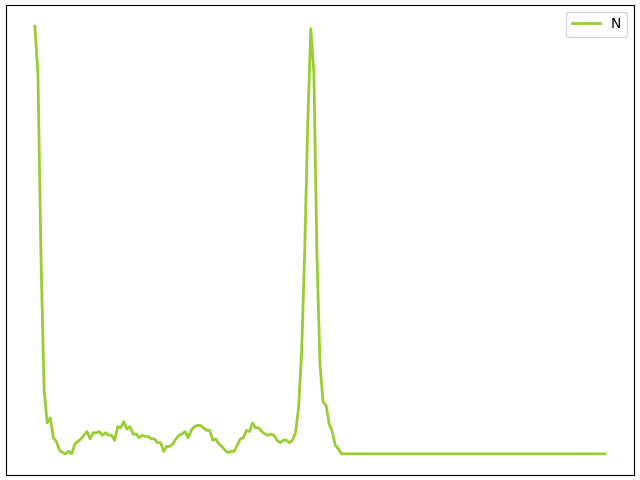
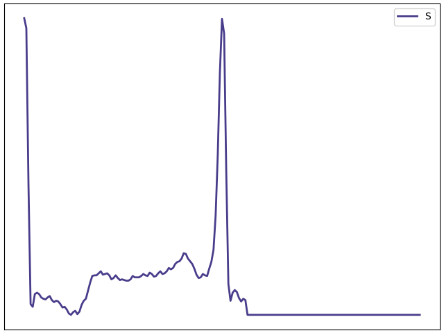
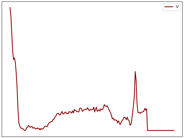
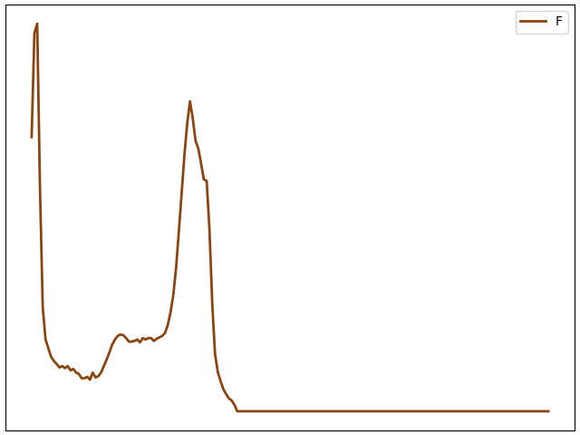
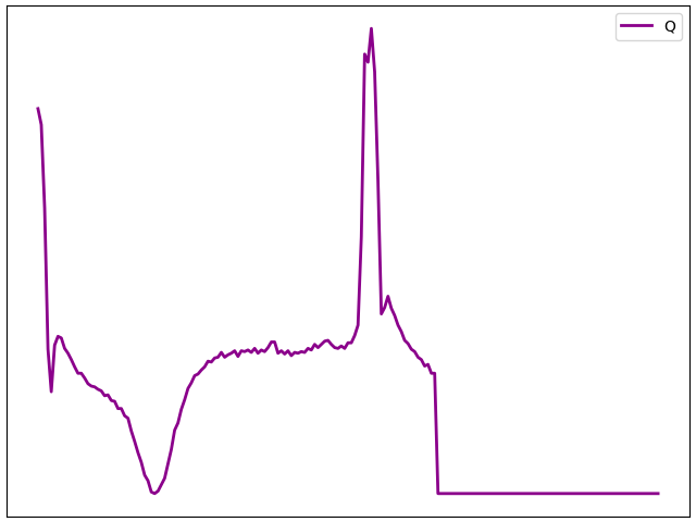
Figure 1: Five classes of ECG beat: {‘N’: normal, left/right bundle branch block, atrial escape, nodal escape}, {‘S’: atrial premature, aberrant atrial premature, nodal premature, supra-ventricular premature}, {‘V’: premature ventricular contraction, ventricular escape}, {‘F’: fusion of ventricular and normal}, {‘Q’: paced, fusion of paced and normal, unclassifiable}.

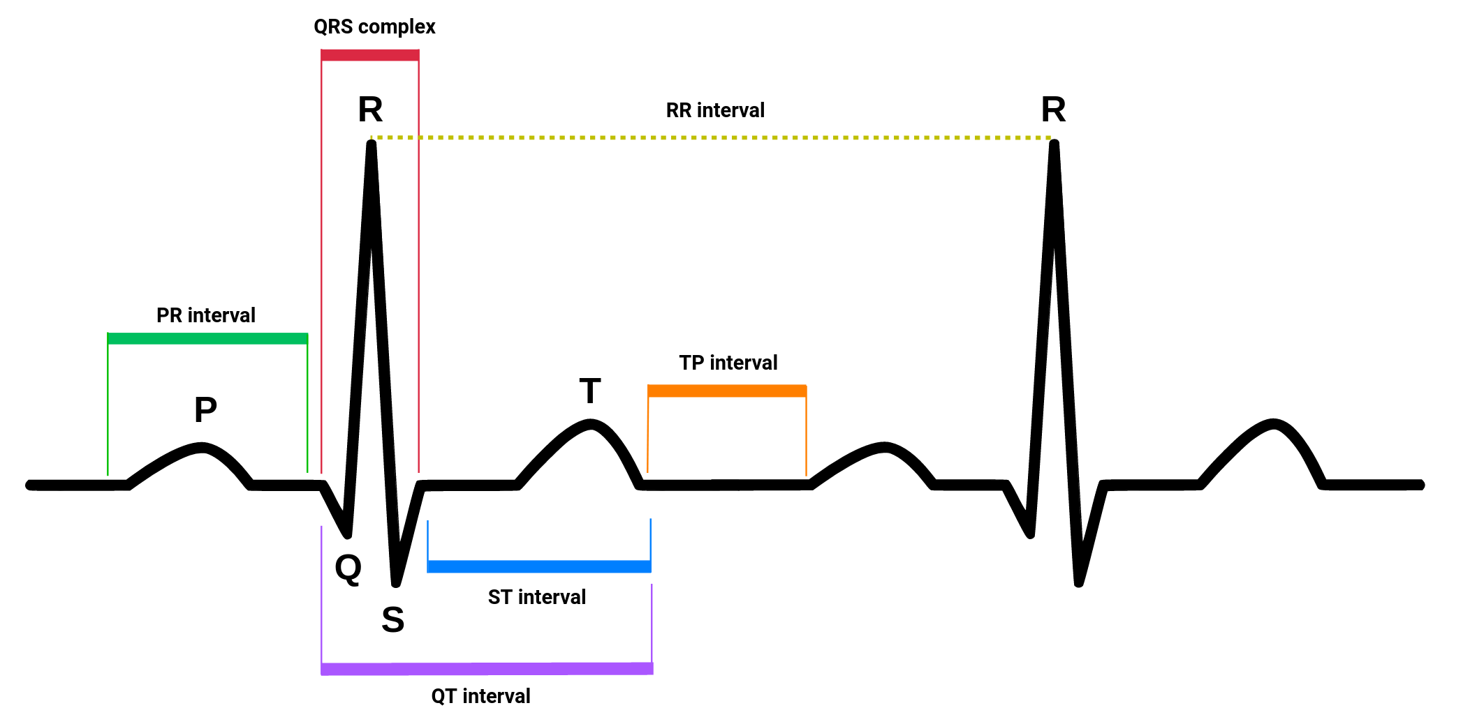
Figure 2: A typical ECG signal with its most common waveforms, where important points and intervals are marked.

Broadly speaking, The existing ECG diagnosis methods in the literature can be categorized into two: conventional machine learning (ML) and deep learning (DL) methods. Conventional ML methods first extract manually-crafted features based on ECG background knowledge and some signal morphological technique, including the QRS complex, T wave, R-R interval, S-T interval (Wasimuddin et al., 2020); see Figure 2. Next, conventional classification methods, such as support vector machines (SVMs; Cortes and Vapnik (1995)), random forest (Breiman, 2001), and gradient boosting (Friedman, 2001), can be used to implement ECG diagnosis under a supervised learning framework based on extracted features (Jambukia, Dabhi and Prajapati, 2015). However, conventional methods strongly depend on the quality of the manually-defined features, which are limited by existing domain knowledge. Specifically, the manually-crafted morphological features may not be able to capture all predictive information in the original ECG signals (Bharti et al., 2021; Thygesen et al., 2007). Moreover, it is also challenging to perfectly extract morphological features from ECG signals due to electrical noise caused by tray magnetic fields and accessories that vibrate (Elgendi, 2013). Therefore, certain biases may be introduced during feature engineering, thus hampering the accuracy of ECG diagnosis.

Recently, deep learning has garnered considerable success in ECG diagnosis. DL differs from conventional ML methods in directly fitting a neural network based on raw ECG signals without feature engineering to extract manual-crafted features. DL models have recently delivered superior performance in the classification of ECG diagnosis. For instance, existing convolutional neural networks (Attia et al., 2019; Rajpurkar et al., 2017; Ko et al., 2020) achieved over 93% heartbeat classification accuracy. In contrast to conventional ML methods, DL models can effectively and adaptively extract the underlying information from raw data. Alternatively, the DL models may localize some novel discriminative features that even ECG experts may not be aware of nor can discern. However, despite their merits, DL models are often referred to as a blackbox, referring to the seeming mystery of their decision-making processes. The lack of interpretable features relevant to the prediction stands out as a significant barrier to the clinical use of their routine. Therefore, our primary goal is to develop a localization framework to unmask unknown discriminative features of blackbox models to help bridge the bench-to-bedside gap and explore the domain knowledge of interpreting ECGs.

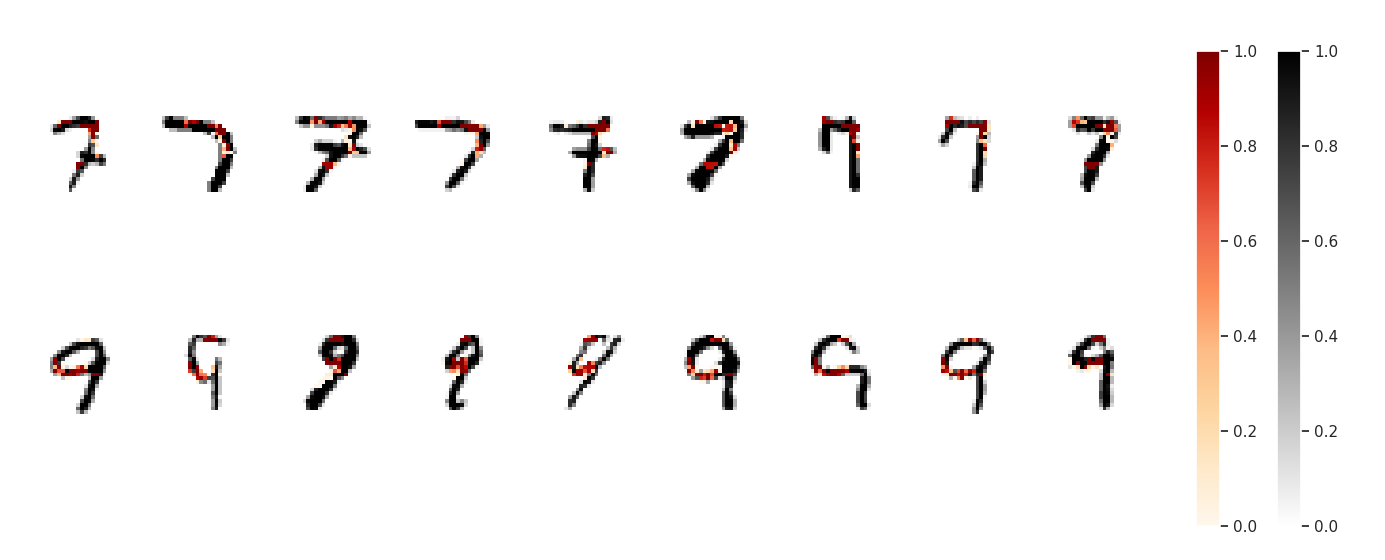
Figure 8: Data-adaptive localized discriminative features (red) for the proposed method with $\tau=20$ based on different ‘7’ and ‘9’ digits (black). The gray color-bar indicates gray scale of original images, and the red color-bar indicates the proportion.

Discriminative feature localization for DL models is important but challenging. The major difficulties include (i) discriminative features are data-dependent on an input instance. For example, in the MNIST or ECG dataset, the location of discriminative features may differ with inputs; see Figures 8 and 10. On this premise, classical variable selection methods based on tabular data are unsuitable without modification; instead, it requires data-adaptive feature selection. (ii) A reliable statistical measure supported by theory is required to quantify predictive importance of any discriminative feature. Most existing methods are heuristic and fail to interpret the localized features. (iii) As indicated in Figure 3, the localized features should effectively explain the discrimination of different outcomes. Hence, effectiveness and predictive importance should be simultaneously considered for selecting sensible discriminative features.

1.2 Prior work and our contributions

Three major approaches have emerged for discriminative feature localization, including two-stage methods, feature-importance-based methods, and backtracking methods. Specifically, two-stage methods use a simple explainable model, such as a local linear model, to approximate a complex blackbox model, and then to extract discriminative features. In particular, a method called local interpretable model-agnostic explanations (LIME) (Ribeiro, Singh and Guestrin, 2016) approximates a classification model by a local sparse linear model based on a kernel smoother as in Davis, Lii and Politis (2011), then highlights those features with positive linear coefficients. Deep-Taylor (Montavon et al., 2017) expands and decomposes a neural network output in terms of its input variables and generates a heatmap by back-propagating explanations from output to input. Feature-importance-based methods rank each feature’s contribution by its importance based on an approximating model in a two-stage method. For example, SHAP (SHapley Additive exPlanations) (Lundberg and Lee, 2017) develops a kernel method integrating LIME with the SHAP-value as the kernel weights and feature importance to quantify the contribution of features in an approximating local linear model. The backtracking methods map the activation layers of a neural network back to the input feature space, identifying which input patterns contribute more to prediction. In particular, Zhou et al. (2016) uses the global average pooling (GAP) together with class activation mapping (CAM) at the last layer of a convolutional neural network (CNN). Then it backtracks discriminative regions at the previous convolutional layers to the predicted scores. Gradient-CAM (Selvaraju et al., 2017) extends GAP to a general CNN model by computing the gradient of a decision score concerning the feature activation maps of a convolutional layer. Deconvnet (Zeiler and Fergus, 2014) and Layer-wise Relevance Propagation (LRP) (Bach et al., 2015) perform backtracking with a deconvolution and conservative relevance redistribution, respectively. Finally, Patternnet (Kindermans et al., 2017) identifies discriminative features by localizing the signal and noise directions for each neuron of a neural network.

Despite their merits, issues remain. First, a two-stage approach does not directly interpret an original model since discriminative features are localized by a simple approximation. For example, discriminative features generated by a linear approximation model (Ribeiro, Singh and Guestrin, 2016; Lundberg and Lee, 2017) may be neither discriminative nor interpretable in the original model. Second, most existing methods are heuristic. As argued in Tjoa and Guan (2019), an intermediate backtracking process for GAP, Gradient-CAM and LRP are not amenable to scrutiny. Moreover, Deconvnet and LRP fail to produce a theoretically correct explanation even for a linear model (Kindermans et al., 2017). Finally, the above methods usually provide a dense representation of discriminative features, as suggested in Figure 9, yielding less effective interpretation.

There are three key contributions of our work in this paper:

• We propose a generalized partial $R^{2}$ in Definition 2.1 to quantify the degree of predictive importance of discriminative features so that they can be interpreted similarly as in classical statistical analysis.

• The proposed localization framework (5) is able to simultaneously consider both predictive importance and effectiveness. Specifically, as illustrated in Figures 7 and 10, it provides a flexible framework to localize discriminative features corresponding to a certain amount of accuracy, as measured by an $R^{2}$.

• Through numerical experiments in Section 5 (the MNIST dataset), the localized discriminative features not only confirm the visual intuition but also are more efficient than the other existing methods. The numerical experiments in Section 6 suggest that localized ECG features are biologically plausible and consistent with cardiac electrophysiological principles, while locating subtle anomalies in sinus rhythm that may not be discernible by the naked eyes.

2 Generalized partial $R^{2}$ for discriminative localization

In this section, we introduce generalized partial ${R}^{2}$ to quantify the degree of predictive importance of discriminative features.

2.1 Motivation

In a learning paradigm, a prediction function $d$ is trained to predict an outcome $Y$ for a given instance $\bm{X}$, where $\bm{X}=(X_{1},\cdots,X_{p})^{\intercal}$ is a $p$-dimensional continuous feature vector. Without loss of generality, each feature component $X_{j}$ is rescaled to $[0,1]$. For example, in the MNIST dataset, $\bm{X}$ is a gray-scale image, and $Y$ is its associated digit label (LeCun and Cortes, 2010). To assess the performance, a loss function $L(\cdot,\cdot)$ is used, such as the cross-entropy loss $L(d(\bm{X}),Y)=-\bm{1}^{\intercal}_{Y}\log\big{(}\text{softmax}\big{(}d(\bm{X})\big{)}\big{)}$, where $\bm{1}_{Y}$ is the one-hot encoding of $Y$ and $\text{softmax}(\bm{z})=(\text{softmax}(\bm{z})_{1},\cdots,\text{softmax}(\bm{z})_{p})^{\intercal}$ with $\text{softmax}(\bm{z})_{i}={\exp(z_{i})}/{\sum_{j}\exp(z_{j})}$.

Our goal is to identify discriminative features that effectively disrupt or deteriorate the prediction performance of a given learner $d$. To proceed, we highlight three distinctive characteristics of discriminative features motivated from real applications, namely adaptiveness, predictive importance, and effectiveness. As an illustrative example based on the MNIST dataset, consider two localized feature sets in the left panel of Figure 3. The feature set removed in the middle or right panel decreases the predictive accuracy of $d$ by the same amount from 0.986 to 0.614, which suggests that the discriminate features should contribute largely to the predictive performance of $d$. Moreover, with the same amount of deterioration of performance, the highlighted features in the middle panel appear more compact, which we call more effective in the sequel, and thus more preferred as discriminative features. Furthermore, key characteristics are also captured by the MIH-BIH data. In particular, the amplitudes and locations of the QRS complexes (Kusumoto, 2020), as well as of P and T waves, varying across ECG signals even of the same class, dictate that the discriminative features should be adaptive to the input ECG signals, as shown in the right panel of Figure 3. Note that the QRS complex corresponds to the spread of a stimulus through the ventricles and is usually the most visually important part of an ECG tracing (Kusumoto, 2020). Moreover, ion channel aberrations and structural abnormalities in the ventricles can affect electrical conduction in the ventricles (Rudy, 2004), manifesting with subtle anomalies in the QRS complex in sinus rhythm that may not be discernible by the naked eyes, yielding sparse or effective discriminative features.

 

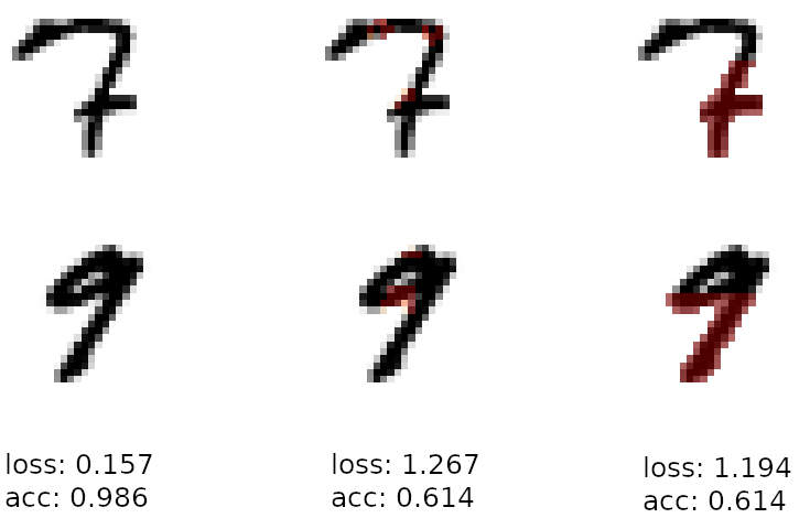
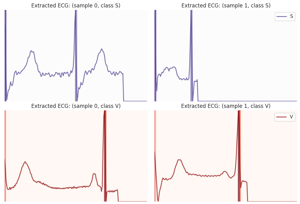
Figure 3: Examples to illustrate the concepts of adaptiveness, predictive importance, and effectiveness of discriminative features on the MNIST and MIT-BIH data. Upper panel. The left represents raw images of digits 7 and 9, the middle represents images with localized pixels (marked in red) by the proposed method, and the right represents images with localized pixels from row 15 to 28. Here ‘loss’ and ‘acc’ denote the cross-entropy and classification accuracy of a conventional neural network for each of the original and two disrupted dataset (by removing the localized regions of all images). Lower panel. The top and bottom each show two extracted ECGs and their localized regions from class ‘S’ (blue) or ‘V’ (red) in the MIT-BIH data. Specifically, the red/blue solid lines are the extracted ECG signals, and the highlighted vertical blue/red bars are localized regions by the proposed method. More discussion can be found in Sections 5 and 6.

In summary, three distinctive characteristics of discriminative features are desired:

• Adaptiveness. Discriminative feature extraction has to be adaptive to an input instance and a specific learner $d$. For example, in the MNIST/MIT-BIH dataset, the location of discriminative features may differ with input images/signals.

• Predictive importance. The prediction accuracy of a learner $d$ would significantly deteriorate without discriminative features. Alternatively, discriminative features can explain a large proportion of its predictive performance.

• Effectiveness. Discriminative features should effectively describe the discrimination of the outcome. Therefore, under the same predictive importance, the number/amount of localized discriminative features should be as small as possible. For example, compact localized pixels in the MNIST dataset or compact and accurate location of QRS complexes of ECG signals in the MIT-BIH ECG dataset.

To address adaptiveness, we introduce a localizer $\bm{\delta}(\bm{x})=(\delta_{1}(\bm{x}),\cdots,\delta_{p}(\bm{x}))^{\intercal}:\mathbb{R}^{p}\to\mathbb{R}^{p}$ to produce a disruption adaptively based on an instance $\bm{x}$ to yield disrupted features $\bm{x}_{\bm{\delta}}=\bm{x}-\bm{\delta}(\bm{x})$. Without loss of generality, assume that each $|\delta_{j}(\bm{x})|\leq 1$ because $x_{j}$ is rescaled to be in $[0,1]$. In practice, the restriction $|\delta_{j}(\bm{x})|\leq 1$ is usually met by construction, for example, in an auto-encoder in image classification, see Section 3.2 for illustration.

2.2 Generalized partial $R^{2}$

To measure the degree of predictive importance of a localizer $\bm{\delta}(\cdot)$, we introduce a generalized partial $R^{2}$, which mimics the partial $R^{2}$ in regression (Nagelkerke et al., 1991) and McFadden’s $R^{2}$ (McFadden et al., 1973) in classification. Specifically, the main idea of the partial $R^{2}$ is one minus the ratio of the full-model risk to the partial model risk. On this ground, we generalize the partial $R^{2}$ to blackbox models in Definition 1.

Definition 2.1 (Generalized partial $R^{2}$).

Given a predictive model $d$, we define the generalized partial $R^{2}$ based on a localizer $\bm{\delta}(\cdot)$ as

$$R^{2}(d,\bm{\delta})=1-\frac{\mathbb{E}\big{(}L(d(\bm{X}),Y)\big{)}}{\mathbb{E}\big{(}L(d(\bm{X}_{\bm{\delta}}),Y)\big{)}}.$$ (1)

If $R^{2}(d,\bm{\delta})\geq r^{2}$, we say that the localized features by $\bm{\delta}(\cdot)$ is $r^{2}$-discriminative.

The generalized partial $R^{2}$ is one minus the proportion of the risk on full features $\bm{X}$ over that of the disrupted features $\bm{X}_{\delta}=\bm{X}-\bm{\delta}(\bm{X})$. It is a natural and clear criterion to extend the classical $R^{2}$, and measure the predictive importance of the features disrupted by a localizer. Specifically, a higher $R^{2}$ yields stronger predictive importance of the localized discriminative features. When $\bm{\delta}(\bm{x})$ does not affect the performance of $d$, that is, $\mathbb{E}\big{(}L(d(\bm{X}_{\bm{\delta}}),Y)\big{)}=\mathbb{E}\big{(}L(d(\bm{X}),Y)\big{)}$, or $R^{2}(d,\bm{\delta})=0$, the localized features contain no information for prediction. On the other hand, $r_{\max}^{2}=\max_{\bm{\delta}}R^{2}(d,\bm{\delta})$ the largest $R^{2}$ among all possible localizers, gives an upper bound of $R^{2}$. For instance, a localizer with each $\delta_{j}(\bm{x})=\bm{x}_{j}$ disrupts extremely by removing all features, which forces a learner $d$ to predict without features. In general, $0<R^{2}<r_{\max}^{2}$ indicates the percentage of performance explained by $\bm{\delta}$.

3 Methods

Our main idea of identifying effective discriminative features is to seek a localizer $\bm{\delta}(\bm{x})$ yielding the most effective disruption of the features to reduce the prediction accuracy of a learner $d$.

3.1 A discriminative localization framework

In Figure 3, the $r^{2}$-discriminative localizer in the right panel is ineffective, although it also affects the same amount of prediction accuracy. Therefore, discriminative features should have an effective (or compact) representation, in addition to their contribution to a learner’s prediction accuracy.

To achieve this goal, we introduce an activity $L_{1}$-regularizer $J(\bm{\delta})$ to quantify the effectiveness of a localizer,

$$J(\bm{\delta})=\sup_{\bm{x}}\sum_{j=1}^{p}\big{|}\delta_{j}(\bm{x})\big{|}.$$ (2)

The benefits of this regularizer are two folds. First, it coincides with greedy feature selection results as indicated in Appendix A. Second, the supremum in (2) makes the localized features more balance over an entire sample, as suggested in Section 5. Moreover, we specify $\|\bm{\delta}(\bm{x})\|_{\infty}\leq 1$ for any $\bm{x}$, to control the magnitude of the disruption. This requirement can be trivially satisfied, for instance, using the proposed truncated rectified linear unit (TReLU) or Tanh as an activation function in the output layer of any deep neural network, see (9) in Section 3.2.

Next, we define an effective $r^{2}$-discriminative localizer $\bm{\delta}^{0}$ as the one minimizing $J(\bm{\delta})$ among all $r^{2}$-discriminative localizers. Then $\bm{\delta}^{0}$ can be regarded as an optimal localizer for identifying discriminative features to interpret a learner’s predictability through effective disruption.

Definition 3.1 (Effective $\bm{r}^{2}$-discriminative).

For $0\leq r^{2}\leq r^{2}_{\max}$, an effective $r^{2}$-discriminative localizer to $d$ is defined as

$$\bm{\delta}^{0}\in\mathop{\rm argmin}_{\bm{\delta}\in\mathcal{H}_{b}:R^{2}(d,\bm{\delta})\geq r^{2}}\ J(\bm{\delta}),$$ (3)

where $\mathcal{H}_{b}$ is a candidate collection of localizers such that $\sup_{\bm{x}}\|\bm{\delta}(\bm{x})\|_{\infty}\leq 1$, and we say that the localized features by $\bm{\delta}^{0}(\cdot)$ is effective $r^{2}$-discriminative.

As noted in Definition 3.1, $\bm{\delta}^{0}$ is a most effective localizer that minimizes the regularization $J(\cdot)$ among all $r^{2}$-discriminative localizers. Without loss of generality, we assume that $\bm{\delta}^{0}$ always exists but may not be unique in the sequel. Note that in the presence of multiple global minimizers in (3), each of them could be useful, since our goal is to estimate such an effective $r^{2}$-discriminative localizer.

To identify an effective discriminative localizer for a learner $d$, we maximize $R^{2}(d,\bm{\delta})$ or the prediction risk $\mathbb{E}\big{(}L\big{(}d(\bm{X}-\bm{\delta}(\bm{X})),Y\big{)}\big{)}$ with respect to $\bm{\delta}$, under the restriction of $J(\bm{\delta})$. This leads to our proposed framework:

$$\max_{\bm{\delta}\in\mathcal{H}_{b}}\ \mathbb{E}\big{(}L\big{(}d(\bm{X}-\bm{\delta}(\bm{X})),Y\big{)}\big{)},\ \text{subject to}\ J(\bm{\delta})\leq\tau,$$ (4)

where $\tau>0$ is a tuning parameter to balance the objective of deteriorating the prediction performance and magnitude of a localizer $\bm{\delta}(\cdot)$. To make the constraint sensible, we let $\tau\leq p$ since $\sup_{\bm{\delta}\in\mathcal{H}_{b}}J(\bm{\delta})=p$. As shown in Lemma 3.2, a most effective $r^{2}$-discriminative localizer $\bm{\delta}^{0}$ can be identified by (4).

Lemma 3.2.

Let $\bm{\delta}^{0}_{\tau}$ be a global maximizer of (4), and

$$\tau^{0}=\min\{\tau\in(0,p]:R^{2}(d,\bm{\delta}^{0}_{\tau})\geq r^{2}\},$$

then $\bm{\delta}^{0}_{\tau^{0}}$ is an effective $r^{2}$-discriminative localizer with $J(\bm{\delta}^{0}_{\tau^{0}})=\tau^{0}$.

Lemma 3.2 says that (4) recovers an effective $r^{2}$-discriminative localizer defined in Definition 3.1 in a similar fashion as Fisher consistency in classification (Lin, 2004; Bartlett, Jordan and McAuliffe, 2006).

Given a training sample $(\bm{x}_{i},y_{i})^{n}_{i=1}$, we propose an empirical risk function to estimate $\bm{\delta}^{0}_{\tau}$ and $\tau^{0}$:

$$\max_{\bm{\delta}\in\mathcal{H}_{b}}\ L_{n}(d,\bm{\delta}) =\frac{1}{n}\sum_{i=1}^{n}L\big{(}d\big{(}\bm{x}_{i}-\bm{\delta}(\bm{x}_{i})\big{)},y_{i}\big{)},\quad\text{subj to,}\quad J(\bm{\delta})\leq\tau.$$ (5)

Denote $\widehat{\bm{\delta}}_{\tau}$ as a maximizer of (5) for a given $\tau$. In view of Lemma 3.2, our final estimate of $(\bm{\delta}^{0}_{\tau^{0}},\tau^{0})$ is

$$\widehat{\bm{\delta}}_{\widehat{\tau}}\text{ is a maximizer of \eqref{eqn:emp_model}},\quad\text{where}\ \widehat{\tau}=\min\{\tau\in(0,p]:R^{2}(d,\widehat{\bm{\delta}}_{\tau})\geq r^{2}\}.$$ (6)

In practice, $\tau\in(0,p]$ is replaced by $\tau\in\bm{\tau}$, where $\bm{\tau}$ is the candidate set of the tuning parameter $\tau$ as some grid points for positive real numbers, and the estimated $R^{2}$ is evaluated based on an independent test sample $\mathcal{D}_{\text{test}}=(\bm{x}_{i},y_{i})^{n+m}_{i=n+1}$,

$$\widehat{R}^{2}(d,\widehat{\bm{\delta}}_{\tau};\mathcal{D}_{\text{test}})=1-\frac{\sum_{(\bm{x},y)\in\mathcal{D}_{\text{test}}}L(d(\bm{x}),y)}{\sum_{(\bm{x},y)\in\mathcal{D}_{\text{test}}}L(d(\bm{x}-\widehat{\bm{\delta}}_{\tau}(\bm{x})),y)}.$$ (7)

Taken together, we iteratively solve (5) for $\tau\in\bm{\tau}$ from the smallest to the largest via a grid search (Bergstra and Bengio, 2012), and it terminates once $\widehat{R}^{2}(d,\widehat{\bm{\delta}}_{\tau};\mathcal{D}_{\text{test}})$ exceeds a prespecified target $r^{2}$.

3.2 A convolutional auto-encoder discriminative localizer

The proposed framework (5) admits a general localizer, such as a deep neural network. In practice, a network architecture incorporating data structure would be preferred (Bengio, 2012). For example, for the image-to-image localization in the MNIST dataset, or the sequence-to-sequence localization in the ECG dataset, convolutional auto-encoder architectures are natural options to impose a “local smoothing” structure of the localized features. Therefore, this section illustrates the localizer $\bm{\delta}$ as a convolutional auto-encoder. It is noted that the network architecture of a discriminative model sets a standard for designing a localizer’s architecture.

Consider a localizer of the form $\bm{\delta}(\bm{x})=\bm{x}\odot\bm{\pi}(\bm{x})$, $\bm{x}$ is an image, where $\odot$ is the element-wise product and $0\leq\bm{\pi}(\bm{x})\leq 1$ represents the percentage of image features that a localizer removes from the original feature $\bm{x}$.

Subsequently, we implement our proposed localizer by taking an image $\bm{x}$ as input and giving output as disruption proportion $\bm{\pi}(\bm{x})$. Specifically, we build a convolutional auto-encoder discriminative localizer based on a convolutional auto-encoder network (CAE; Masci et al. (2011); Rumelhart, Hinton and Williams (1985)), which is composed of three components: Encoder-CNN (E-CNN), hidden neural network (HNN), and Decoder-CNN (D-CNN), as illustrated in Figure 4. Besides, on the CAE backend model, we introduce a TReLU-softmax or Tanh+ReLU-softmax activation function to control the activity $L_{1}$-regularizer of the localizer. On this ground, we consider a localizer class:

$$\mathcal{H}^{\tau}_{b}=\Big{\{}\bm{\delta}_{\tau}(\bm{x})=\bm{x}\odot\bm{\pi}_{\bm{\theta}}^{\tau}(\bm{x}):\bm{\pi}_{\bm{\theta}}^{\tau}(\bm{x})=A_{\tau}\big{(}\text{CAE}_{\bm{\theta}}(\bm{x})\big{)};\ \bm{\theta}\in\bm{\Theta}\Big{\}},$$ (8)

where $\text{CAE}_{\bm{\theta}}(\bm{x})$ is a convolutional auto-encoder with $\bm{\theta}\in\mathbb{R}^{q}$ denoting its parameters, $\bm{\Theta}$ is a parameter space of $\bm{\theta}$, and $A_{\tau}(\cdot)$ is a structured activation function, such as:

$$A_{\tau}(\bm{z})=\text{TReLu}\big{(}\tau\cdot\text{softmax}(\bm{z})\big{)},\text{ or }A_{\tau}(\bm{z})=\text{Tanh}\Big{(}\text{ReLu}\big{(}\tau\cdot\text{softmax}(\bm{z})\big{)}\Big{)}$$ (9)

where $\text{TReLu}(\bm{u})=\min(\bm{u}_{+},\bm{1})$ is the truncated ReLU function.

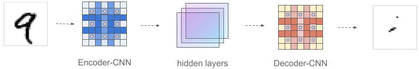
Figure 4: Our localization network structure based on a convolutional auto-encoder, which is composed of three components: Encoder-CNN (E-CNN), hidden neural network (HNN), and Decoder-CNN (D-CNN).

Note that for any $\bm{\delta}\in\mathcal{H}^{\tau}_{b}$, based on the definition of $A_{\tau}$, the following conditions are automatically satisfied: (i) $\sup_{\bm{x}}\|\bm{\delta}(\bm{x})\|_{\infty}\leq 1$; (ii) $J(\bm{\delta})=\sup_{\bm{x}}\|\bm{\delta}(\bm{x})\|_{1}\leq\tau$. Therefore, the constraints in (5) can be removed given $\mathcal{H}^{\tau}_{b}$, and the optimization of (5) becomes:

$$\max_{\bm{\theta}}\ \frac{1}{n}\sum_{i=1}^{n}L\big{(}d\big{(}\bm{x}_{i}-\bm{x}_{i}\odot\bm{\pi}^{\tau}_{\bm{\theta}}(\bm{x}_{i})\big{)},y_{i}\big{)},$$ (10)

which can be solved by Gradient Descent (GD) or stochastic gradient descent (SGD; Raginsky, Rakhlin and Telgarsky (2017)). The GD solution of (10) attains a local maximizer of (10) under some mild assumptions (Lee et al., 2016). Note that the convergence result can be extended to SGD as in (Ge et al., 2015), and a global maximizer may be obtained by GD or SGD with additional assumptions (Raginsky, Rakhlin and Telgarsky, 2017). Once $\widehat{\bm{\theta}}$ is obtained, the estimated localizer is specified as

$$\widehat{\bm{\delta}}_{\tau}(\bm{x})=\bm{x}\odot A_{\tau}\big{(}\text{CAE}_{\widehat{\bm{\theta}}}(\bm{x})\big{)}.$$ (11)

3.3 Interpretation uncertainty

Robustness is a general challenge to existing interpretation approaches. For example, Ghorbani, Abid and Zou (2019) indicates that systematic perturbations can lead to dramatically different interpretations without changing the label. To distinguish the interpretability and robustness for the proposed framework, we propose an unexplainable $R^{2}$ as a confidence interval for the generalized partial $R^{2}$ to distinguish the prediction deterioration caused by discriminative features from model instability. In particular, given a learner $d$ and a localizer $\widehat{\bm{\delta}}_{\tau}$, we construct a confidence interval for $R^{2}(d,\widehat{\bm{\delta}}_{\tau})$ via bootstrap on a test sample.

First we generate a bootstrap sample $\mathcal{D}^{(b)}_{\text{test}}$ by drawing $B$ independent observations from the test data $\mathcal{D}_{\text{test}}$ with replacement. Then the unexplainable $R^{2}$ for $R^{2}(d,\widehat{\bm{\delta}}_{\tau})$ is obtained using the sampling distribution of the bootstrapped estimates $\big{\{}\widehat{R}^{2}(d,\widehat{\bm{\delta}}_{\tau};\mathcal{D}^{(B)}_{\text{test}})\big{\}}_{b=1}^{B}$. For example, for the MNIST dataset, we obtain a 95% confidence interval of $R^{2}(d,\widehat{\bm{\delta}}_{\tau})$ by computing the $\lfloor.025B\rfloor$-th and $\lfloor.975B\rfloor$-th ordered estimated $R^{2}$ on the bootstrap samples, as indicated in Figure 5. More detail can be found in Section 5.

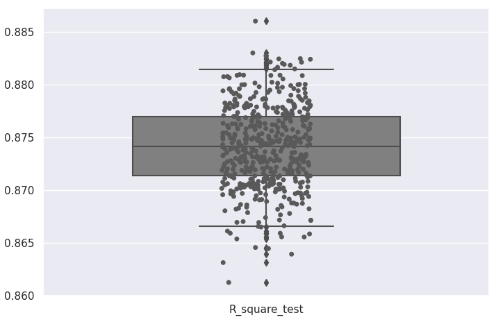
Figure 5: Boxplot of the estimated $R^{2}$ of the proposed method based on 500 bootstrap samples for the MNIST benchmark example. This example illustrates the concept of an unexplainable $R^{2}$.

4 Theoretical guarantee

This section indicates that the proposed framework yields discriminative features attaining a target $R^{2}$ with optimal effectiveness asymptotically.

To proceed, let $\bm{\delta}^{0}_{\tau}$ be a global maximizer of (4) over a function class $\mathcal{H}_{b}=\big{\{}\bm{\delta}\in\mathcal{H}:\ \sup_{\bm{x}}\|\bm{\delta}(\bm{x})\|_{\infty}\leq 1\big{\}}.$ Without loss of generality, assume that $0\leq L(d(\bm{x}_{\bm{\delta}}),Y)\leq U$ for a sufficiently large constant $U\geq 1$, for any $\bm{\delta}\in\mathcal{H}_{b}$ and $\bm{x}\in\mathbb{R}^{p}$ (Wu and Liu, 2007). To make the constraint sensible, we let $\tau\leq p$ since $\sup_{\bm{\delta}\in\mathcal{H}_{b}}J(\bm{\delta})=p$.

Denote the Rademacher complexity for the function class $\mathcal{H}_{b}$ as $\kappa_{n}=\mathbb{E}\mathcal{R}_{n}\big{(}\mathcal{H}_{b}\big{)}=\sup_{\bm{\delta}\in\mathcal{H}_{b}}n^{-1}\sum_{i=1}^{n}\big{|}\eta_{i}\big{(}L(d(\bm{X}_{i}-\bm{\delta}(\bm{X}_{i})),Y)\big{)}\big{|}$, and $\{\eta_{i}\}_{i=1}^{n}$ are i.i.d. Rademacher random variables with $\eta_{i}$ taking the values +1 and -1 with probability 1/2 each. To make the constraint sensible, we let $\tau\leq p$ since $\sup_{\bm{\delta}\in\mathcal{H}_{b}}J(\bm{\delta})=p$. Theorem B.1 gives a convergence rate for the discrepancy between $\bm{\delta}^{0}_{\tau}$ and $\widehat{\bm{\delta}}_{\tau}$ in terms of $R^{2}$ uniformly over $0<\tau\leq p$.

Theorem 4.1 (Asymptotics of $\bm{R}^{2}$).

Let $\widehat{\bm{\delta}}_{\tau}$ be a global maximizer of (5), for $\varepsilon_{n}\geq 8\kappa_{n}$ and any predictive model $d$, we have

$$\mathbb{P}\big{(}\sup_{0<\tau\leq p}R^{2}(d,\bm{\delta}^{0}_{\tau})-R^{2}(d,\widehat{\bm{\delta}}_{\tau})\geq\varepsilon_{n}\big{)}\leq K\exp\big{(}-\frac{n\varepsilon_{n}^{2}}{KU^{2}}\big{)},$$

where $K>0$ is a constant. Hence,

$$\sup_{0<\tau\leq p}(R^{2}(d,\bm{\delta}^{0}_{\tau})-R^{2}(d,\widehat{\bm{\delta}}_{\tau}))=O_{p}\big{(}\max(\kappa_{n},n^{-1/2})\big{)}.$$

Note that the asymptotics of the Rademacher complexity $\kappa_{n}$ for a candidate class $\mathcal{H}$ has been extensively investigated in the literature (Bartlett and Mendelson, 2002; Bartlett, Bousquet and Mendelson, 2005). Therefore, the uniform convergence rate can be obtained for a generic candidate class by Theorem B.1. Moreover, the asymptotics for a fixed $\tau$ is also provided in Appendix C, where the rate can be further improved.

Next, we show that $\widehat{\bm{\delta}}_{\widehat{\tau}}$ is an asymptotically effective $r^{2}$-discriminative localizer. Note that $\widehat{\bm{\delta}}_{\widehat{\tau}}$ already is an $r^{2}$-discriminative localizer, since $R^{2}(d,\widehat{\bm{\delta}}_{\widehat{\tau}})\geq r^{2}$ by the definition of $\widehat{\tau}$ in (6). Therefore, it suffices to show effectiveness, that is, that is, $|J(\widehat{\bm{\delta}}_{\widehat{\tau}})-J(\bm{\delta}^{0}_{\tau^{0}})|=|\widehat{\tau}-\tau^{0}|\overset{p}{\longrightarrow}0$. To proceed, we require a smoothness condition of $R^{2}(d,\bm{\delta}^{0}_{\tau})$ over $\tau$ in Assumption A.

Assumption A (Smooth). Assume that $R^{2}(d,\bm{\delta}^{0}_{\tau})$ is a continuous function in $\tau$. Moreover, there exists a constant $\mu_{0}>0$ such that $|\tau_{1}-\tau_{2}|\leq\mu$ if $|R^{2}(d,\bm{\delta}^{0}_{\tau_{1}})-R^{2}(d,\bm{\delta}^{0}_{\tau_{2}})|\leq c_{0}\mu^{\alpha}$ for any $\mu\leq\mu_{0}$.

Theorem 4.2 (Oracle property).

Let $\bm{\delta}^{0}$ be an effective $r^{2}$-discriminative localizer in Definition 3.1 and $\widehat{\bm{\delta}}_{\widehat{\tau}}$ be a global maximizer of (6). Under Assumption A, for $\omega_{n}\geq 2(8\kappa_{n}/c_{0})^{1/\alpha}$, we have

$$\mathbb{P}\Big{(}\big{|}\widehat{\tau}-\tau^{0}\big{|}\geq\omega_{n}\Big{)} =\mathbb{P}\Big{(}\big{|}J(\widehat{\bm{\delta}}_{\widehat{\tau}})-J(\bm{\delta}^{0})\big{|}\geq\omega_{n}\Big{)}\leq K^{\prime}\exp\Big{(}-\frac{n\omega_{n}^{2\alpha}}{K^{\prime}U^{2}}\Big{)},$$

where $K^{\prime}>0$ is a universal constant. Therefore,

$$|J(\widehat{\bm{\delta}}_{\widehat{\tau}})-J(\bm{\delta}^{0}_{\tau^{0}})|=|\widehat{\tau}-\tau^{0}|\overset{p}{\longrightarrow}0,$$

and $\widehat{\bm{\delta}}_{\widehat{\tau}}$ is an asymptotically effective $r^{2}$-discriminative localizer.

Therefore, the proposed framework yields an effective $r^{2}$-discriminative localizer as defined in (3.1), rendering theoretical reliable discriminative features for a target $R^{2}$. Moreover, the theorems are illustrated for the proposed convolutional auto-encoder neural network (10) in Corollary B.1, where the convergence rates are computed depending on the sample size and the network architecture.

5 MNIST benchmark

This section examines the numerical performance and visualizes discriminative features generated from the proposed localizer for the MNIST handwritten digit dataset (LeCun and Cortes, 2010) (http://yann.lecun.com/exdb/mnist/). All empirical results are produced in our Python library dnn-locate (https://github.com/statmlben/dnn-locate).

For the MNIST data, we extract 14,251 images (28$\times$28 field) from the dataset with labels ‘7’ and ‘9’. Our goal is to localize discriminative features for distinguishing digits ‘7’ and ‘9’ with a specific generalized partial $R^{2}$.

First, we train a decision function $d$ as a CNN, where we regularize each parameter of the CNN by the $L_{1}$-norm with weight 0.001. Here the CNN model is optimized by the Adam algorithm with an initial learning rate of 0.001, early stopping based on the validation accuracy with patience as 10, and 20% of the training data as a validation set.

Then, a convolutional auto-encoder (CAE), as in (8) and Figure 4, is constructed as the localizer. For training, we optimize the model by stochastic gradient descent with an initial learning rate of $10/\tau$ and reduce the learning rate by a factor of 0.382 (Bengio, 2012), when the validation loss has stopped improving. Moreover, early stopping is conducted based on validation accuracy with patience as 15 (Raskutti, Wainwright and Yu, 2014).

For the proposed method, we implement (10) based on $\tau=4,6,8,10,12,14,18,20$, and the relation between $\tau$ and its corresponding estimated $R^{2}$s are demonstrated in Figure 6. Note that the estimated $R^{2}$ increases as the activity $L_{1}$-norm of the localizer becoming large. Furthermore, the discriminative features, identified by the proposed method for two illustrative instances of ‘7’ and ‘9’, are visualized in Figure 7. Specifically, as the estimated $R^{2}$ becomes larger, the disrupted instance labeled as ‘9’ becomes more and more like ‘7’.

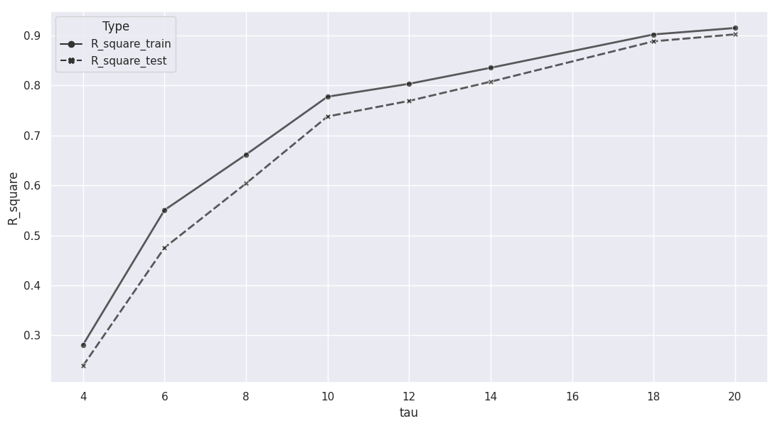
Figure 6: Training and testing estimated $R^{2}$s for the proposed framework in handwritten digit dataset with $\tau=6,8,10,12,14,16,18,20$, which indicates that the $R^{2}$ increases as the magnitude for an estimated localizer becoming large.

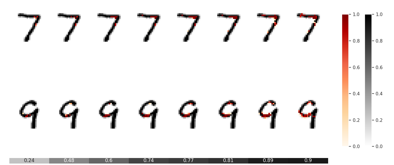
Figure 7: Illustrative instances of localized discriminative features (red) by the proposed method for ‘7’ and ‘9’ digits (black) as well as their corresponding estimated $R^{2}$s (the heatmap in x-axis). The gray color-bar indicates gray scale of original images, and the red color-bar indicates the proportion of removing features, that is, $\bm{\pi}(\bm{x})$ in (10).

As illustrated by the boxplot (Figure 5), a 95% confidence interval [0.867, 0.882] for the $R^{2}(d,\widehat{\bm{\delta}}_{\tau})$ indicates some uncertainty with the fitted localizer ($\tau=17$), where the $R^{2}$ is categorized as unexplainable if it falls inside the confidence interval.

Next, we compare the proposed method with five state-of-the-art methods by both human visual and numerical evaluations, including deep Taylor explainer (Montavon et al., 2017), gradient-based explainer (Selvaraju et al., 2017), lrp.z (Bach et al., 2015), deconvnet (Zeiler and Fergus, 2014), and pattern.net (Kindermans et al., 2017). All competitors are implemented by the Python library innvestigate (https://github.com/albermax/innvestigate), and the batch size is set as 64 for pattern.net. In particular, a heatmap of discriminative features produced by each method is validated by a visual inspection and by a numerical comparison based on the estimated $R^{2}$ given the same amount/magnitude of feature disruption.

5.1 Visual comparison

As displayed in Figure 7, the proposed method produces more compact discriminative features. By comparison, the other competitors yield dense image features spreading over the entire digits. Moreover, the proposed method gives roughly equal attention to two images in discriminating digits ’7’ from ’9’, which conforms with human intuition. However, as depicted in 9, all competitors generate imbalanced discriminative features that are more in one of the two images of ‘7’ and ‘9’ as shown in Figure 9. As a result, the proposed method is more conducive for label-specific analysis.

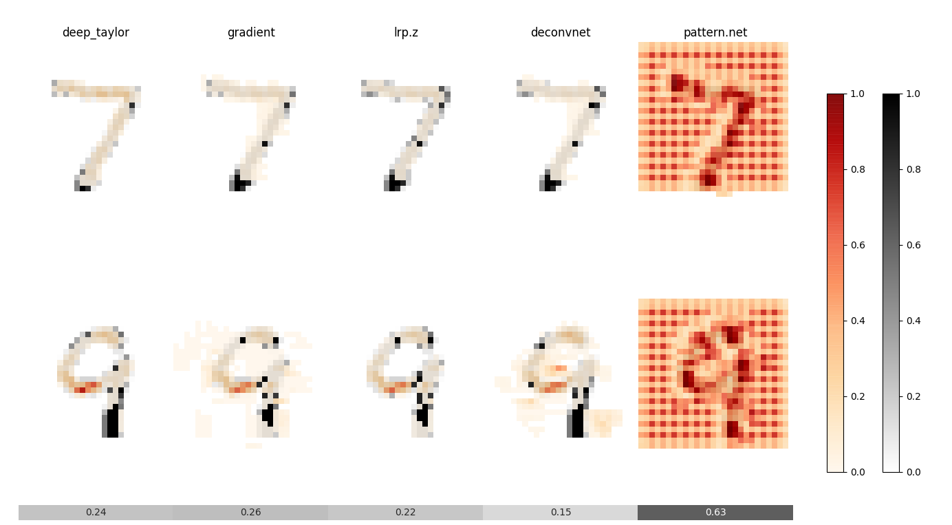
Figure 9: Illustrative instances of localized discriminative features (red), based on five competitors, for ‘7’ and ‘9’ digits (black), and their corresponding generalized partial $R^{2}$s (the heatmap in x-axis). The gray color-bar indicates gray scale of original images, and the red color-bar indicates importance of pixels produced by a localizer.

5.2 Numerical comparison

To make a fair comparison, we conduct a pairwise comparison between the proposed localizer and each competitor under the same magnitude of $J(\cdot)$. Specifically, we compute the value of $J(\cdot)$ and the estimated $R^{2}$ of detected regions by a competitor. To fairness, we chose our tuning parameter $\tau$ to be the same as the $J(\cdot)$ of the competitor. Then compare the $R^{2}$s for the proposed method and the corresponding competitor.

As indicated in Table 1, under the same magnitude $J(\cdot)$, the proposed localizer outperforms all competitors in terms of $R^{2}$, where the amounts of improvement are 58.47%, 147.1%, 146.5%, 308.0%, and 44.14%.

Table 1: A pairwise comparison for the proposed framework and five existing methods based on 10-fold cross validation. Here $J(\cdot)$ is the activity $L_{1}$-regularizer as defined in (2), and the estimated $R^{2}$ as in (7).

			activity $L_{1}$-norm $J(\cdot)$		$\widehat{R}^{2}$ (competitor in the first column)		$\widehat{R}^{2}$ (our method)
	deep-Taylor		11.698(.228)		0.236(.016)		0.374(.084)
	gradient		26.028(.319)		0.289(.012)		0.714(.033)
	lrp.z		14.689(.219)		0.256(.014)		0.631(.077)
	deconvnet		27.832(.955)		0.175(.015)		0.714(.023)
	pattern.net		374.709(2.762)		0.648(.006)		0.934(.001)

In summary, the proposed method has significant benefits. First, as illustrated in Figure 7, it provides a flexible framework to localize desirable discriminative features to explain a certain amount of predictive performance as measured by an $R^{2}$. Second, the visual and numerical results in Figures 7 and 9 and Table 1 suggest that the proposed method can produce compact and effective discriminative features, which are consistent with human visual judgment.

6 ECG data analysis

Finally, we present the results of applying our method to the MIT-BIH Arrhythmia Electrocardiogram (ECG) dataset for heartbeat classification (Moody and Mark, 1990). The MIT-BIH dataset consists of ECG recordings from 47 different subjects recorded at the sampling rate of 360Hz by the BIH Arrhythmia Laboratory. Each beat is annotated into 5 different classes by following the Association for the Advancement of Medical Instrumentation (AAMI) EC57 standard: labeled as ’N’, ’S’, ’V’, ’F’, and ’Q’. The pre-processed dataset is publicly available at https://www.kaggle.com/shayanfazeli/heartbeat. The MIT-BIH ECG dataset has been extensively studied, including using deep convolutional neural networks (Kachuee, Fazeli and Sarrafzadeh, 2018; Acharya et al., 2017; Martis et al., 2013). In spite of the impressive predictive performance obtained by the devised networks (with more than 93% classification accuracy), it is unknown why and how the networks achieved their good performance. To advance our understanding and possibly offering new insights, our goal is to localize discriminative signal fragments based on the deep CNN developed in Kachuee, Fazeli and Sarrafzadeh (2018), which is one of the state-of-the-art ECG classification methods.

For implementation, we build a localizer by using a convolutional auto-encoder structure in Figure 4 with two convolutional layers as an encoder and two transposed convolution layers as a decoder. For training, we use the SGDW optimizer with “learning_rate=.1”, “weight_decay=1e-4”, “momentum=.9”. Besides, a reducing learning rate scheme is used with “factor=.382” and “patience=3”, and early stopping is adopted with “patience=20”. Moreover, we tune the hyperparameter $\tau$ to achieve various $R^{2}$s: 10%, 50%, 60%, 70%, 75%. Training one network takes less than half an hour on a GeForce GTX 2060Ti GPU. All the Python codes are publicly available in https://github.com/statmlben/dnn-locate.

To demonstrate our localization results, we concentrate on the localized ECG signals under the label ‘S’ (including atrial premature, aberrant atrial premature, nodal premature, and supra-ventricular premature) and the label ‘V’ (including premature ventricular contraction, and ventricular escape).

 

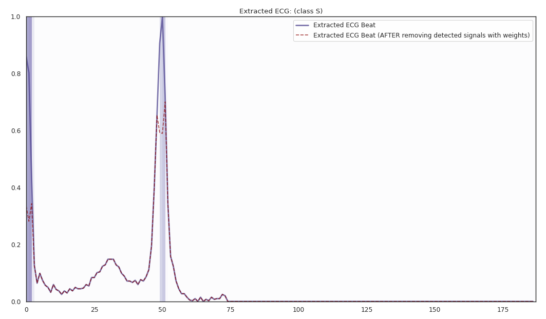
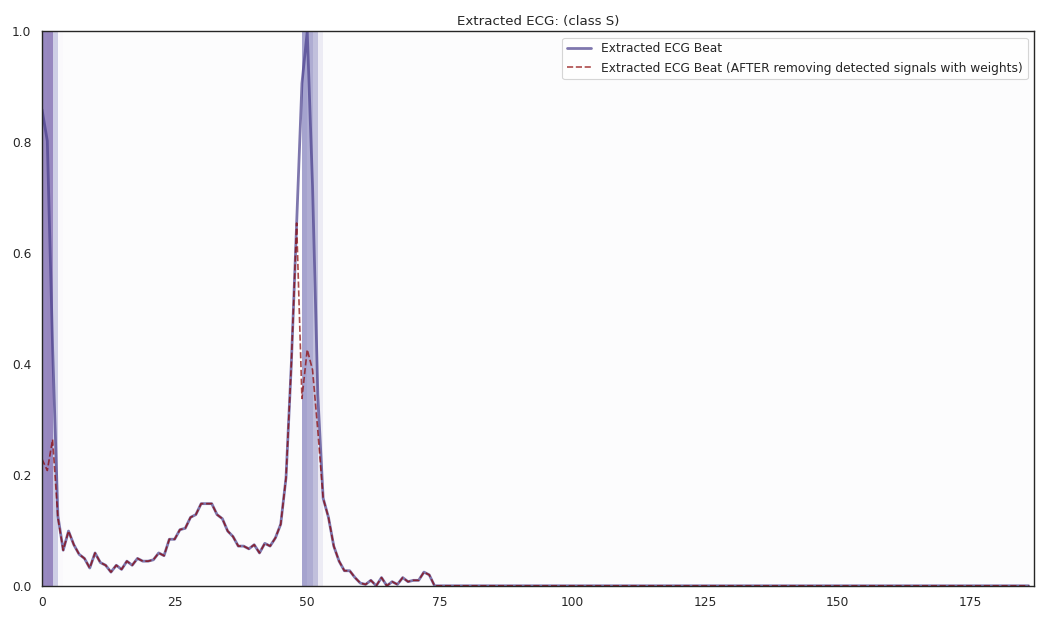
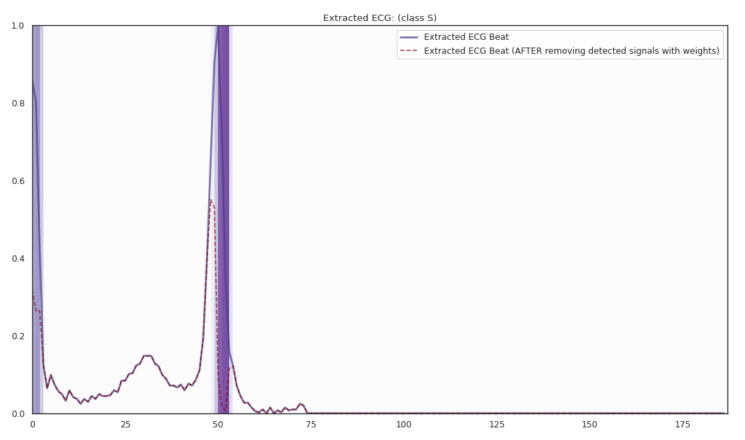
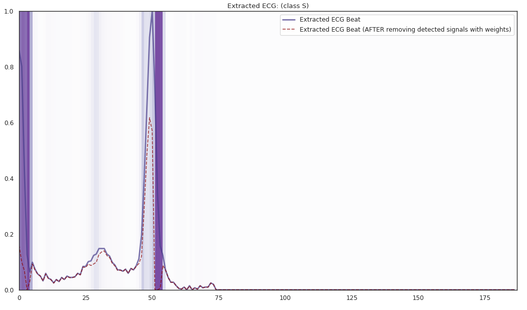
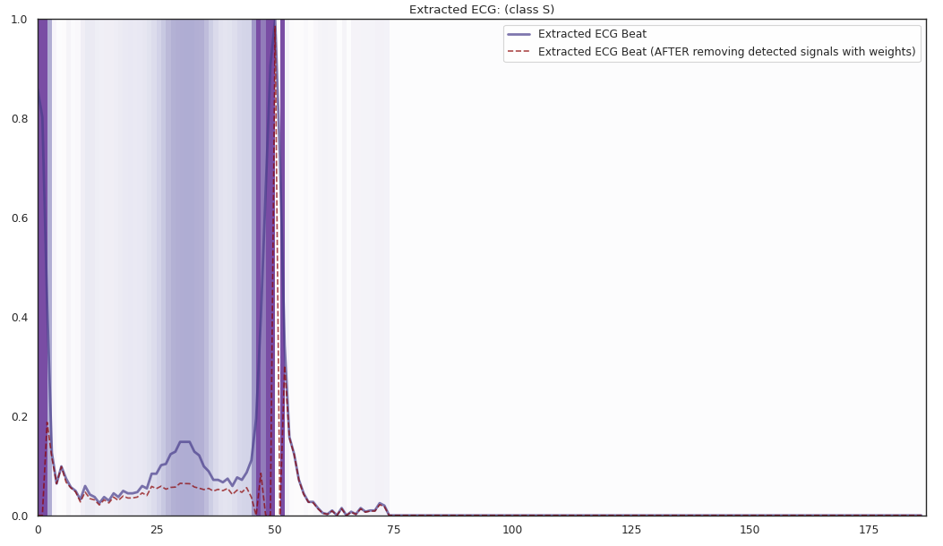
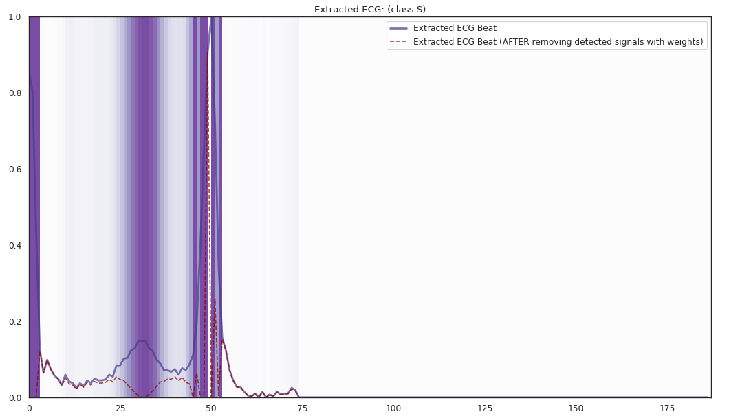
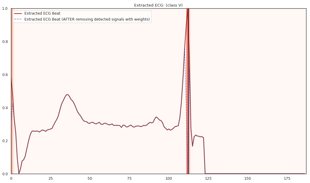
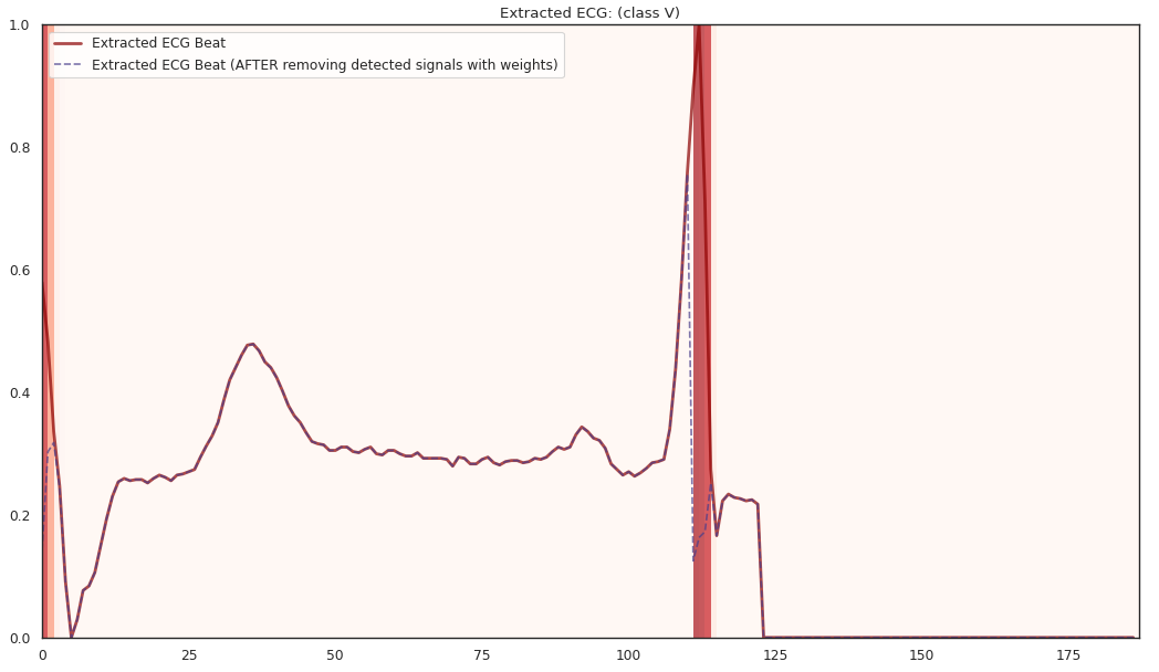
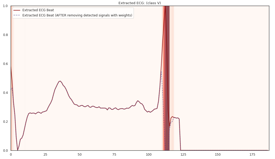
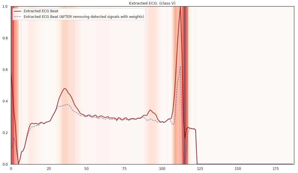
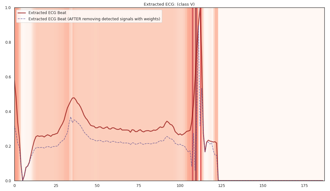
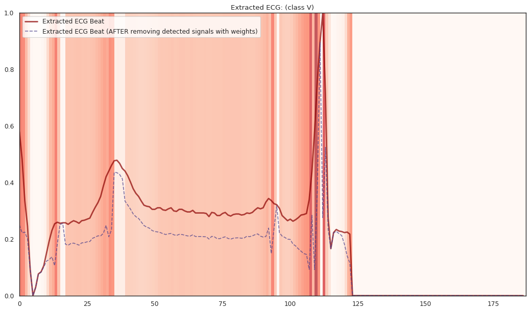
Figure 10: The proposed method reveals subtle discriminative features used by a deep convolutional neural network for ECG classification on the MIT-BIH dataset. The left/right panel highlights the localized features for a particular individual under label ‘V’/‘S’. Note that the $R^{2}$ increases from 10% to 88% for both upper and lower panels. The medical literature provided in Section 6 gives supporting evidence for biological plausibility of the localized features; see more discussion in Section 6.

As shown in the lower panel of Figure 10, the localized regions (highlighted by the red bars) of ECG complexes in sinus rhythm are most informative in distinguishing presence of ventricular ectopic beats from supraventricular ectopic beats in a particular individual. The localized regions lie in the QRS complex, which correlates with ventricular depolarization or electrical propagation in the ventricles (Mirvis and Goldberger, 2001). Ion channel aberrations and structural abnormalities in the ventricles can affect electrical conduction in the ventricles (Rudy, 2004), manifesting with subtle anomalies in the QRS complex in sinus rhythm that may not be discernible by the naked eye but is detectable by the convolutional auto-encoder. Of note, as the $R^{2}$ increases from 10% to 88%, the highlighted color bar is progressively broader, covering a higher proportion of the QRS complex. The foregoing observations are sensible: the regions of interest resided in the QRS complex are biologically plausible and consistent with cardiac electrophysiological principles.

As shown in the upper panel of Figure 10, similarly, the regions of interest (highlighted by the blue bars) of ECG complexes in sinus rhythm are most informative in distinguishing the presence of supraventricular ectopic beats from ventricular ectopic beats in a particular individual. As in the left panel, the regions of interest lies in the QRS complex, which is intuitive and biologically plausible as explained above.

As shown in the last three figures in the upper panel of Figure 10 for supraventricular complexes, as the $R^{2}$ increases from 80% to 84% and finally 88%, the blue bar progressively highlights the P wave of ECG complexes in sinus rhythm. This observation is consistent with our understanding of the mechanistic underpinnings of atrial depolarization, which correlates with the P wave. Ion channel alterations and structural changes in the atria can affect electrical conduction in the atria (Rudy, 2004), manifesting with subtle anomalies in the P wave in sinus rhythm that may not be discernible by the naked eye but are detectable by the convolutional auto-encoder.

Collectively, the examples above underscore the fact that the discriminative regions of interest identified by our proposed method are biologically plausible and consistent with cardiac electrophysiological principles while locating subtle anomalies in the P wave and QRS complex that may not be discernible by the naked eye. By inspecting our results with an ECG clinician (Dr. Chen in the authorship), the localized discriminative features of the ECG are consistent with medical interpretation in ECG diagnosis.

6.1 Robustness against localization network architecture

This section examines the robustness of the proposed framework against network architectures. We use the same implementation configuration with $\tau=0.05$, and examine CAE network architectures with different numbers of neurons, denoted as CAE64, CAE128, CAE256 and CAE512, where CAE64 is constructed as: Conv1D(64)+Conv1D(32)+Conv1DTranspose(32)+Conv1DTranspose(64), and other CAE networks are defined likewise. Moreover, we also implement a localizer with a multilayer perceptron (MLP) structure: MLP256, MLP512, MLP1024, and MLP2048. For example, MLP256 is constructed as: Dense(256)+Dense(128)+Dense(64)+Dense(187), and other MLP networks are defined likewise. As indicated in Table 2, $R^{2}$s of the localized discriminative features provided by convolutional auto-encoders are significantly higher and more stable than those produced by MLPs. In particular, for CAE-based networks, larger networks generally improve the performance. The localization results by the CAE networks are illustrated in Figure 11: the localized discriminative features are fairly consistent with different CAE-based network architectures.

Table 2: $R^{2}$s for the proposed framework with different network architectures. Here “CAE” indicates a convolutional auto-encoder, “MLP” indicates a multilayer perceptron, and the estimated $R^{2}$ is computed as in (7) based on 10-fold cross-validation.

CAE64	CAE128	CAE256		MLP512	MLP1024	MLP2048
0.816(.028)	0.872(.011)	0.872(.015)		0.141(.252)	0.156(.255)	0.133(.242)

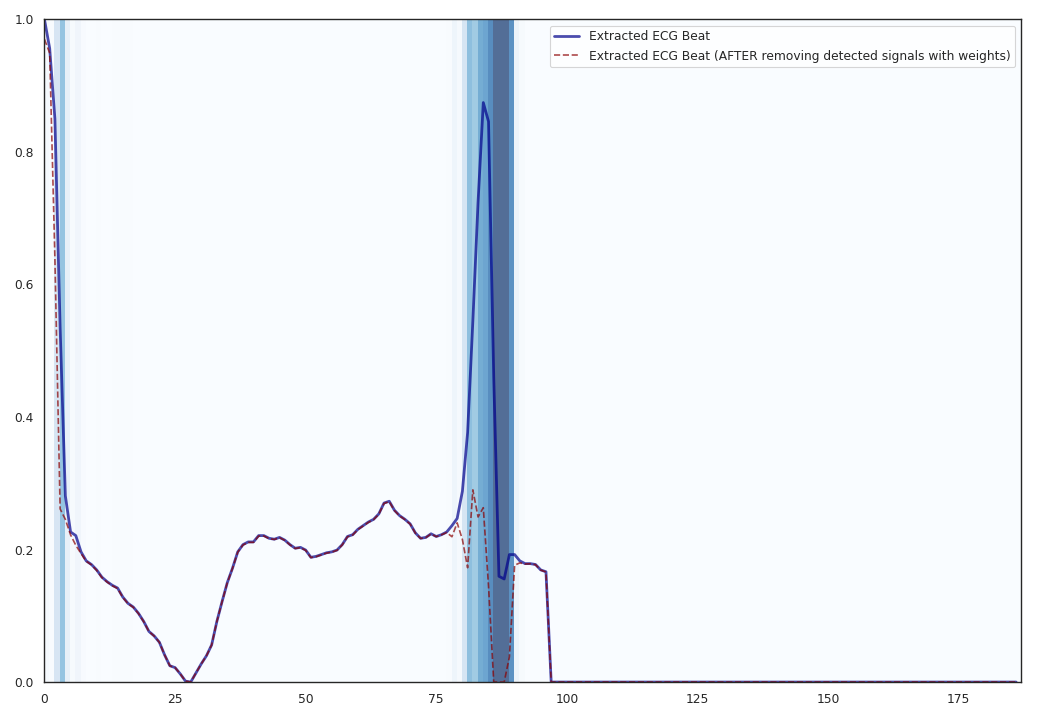
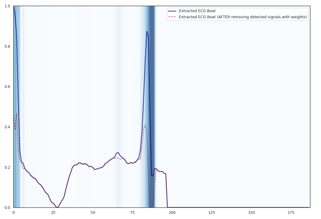
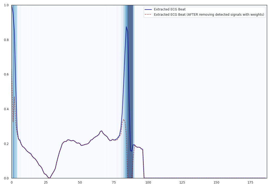
Figure 11: The localized discriminative features of one ECG signal in the MIT-BIH dataset based on the proposed framework with different CAE network architectures: CAE64 - CAE256.

7 Discussion

XAI methods have gained prominence in many scientific domains, for example, medical diagnostics, which requires both interpretability and predictive accuracy. To identify discriminative features, we quantify the quality of interpretability by a generalized partial $R^{2}$ while measuring the interpretation effectiveness by an activity $L_{1}$-norm. On this ground, we construct a localizer by disrupting the original features, and seek a localizer yielding the most deteriorated performance of a learner while having the smallest activity norm for minimal feature disruption. Theoretically, we show that the proposed localization method identifies discriminative features asymptotically. Moreover, we apply the proposed framework to the MNIST and MIT-BIH ECG datasets to interpret a learning outcome of a convolutional auto-encoder neural network. Numerical results suggest that the proposed localizer compares favorably with state-of-the-art competitors in the literature while identifying discriminative regions that are not only visually/biologically plausible but also concise. Furthermore, it is of interest to know if any localized features are genuinely important, for which hypothesis testing targeting a data-adaptive localizer as in Dai, Shen and Pan (2022) would be needed as a possible extension of our framework.

[Acknowledgments] The corresponding authors for this work are Ben Dai and Wei Pan. The authors would like to thank the referees, the Associate Editor, and the Editor for the constructive feedback which greatly improved this work.

We would like to acknowledge support for this project from RGC-ECS 24302422, the CUHK direct grant, NSF DMS-1712564, DMS-1721216, DMS-1952539, and NIH grants R01GM126002, R01AG069895, R01AG065636, R01AG074858, R01AG074858, U01AG073079 and RF1 AG067924.

Supplement to “Data-Adaptive Discriminative Feature Localization with Statistically Guaranteed Interpretation”. The supplementary materials consist of: Appendix A indicates that the proposed framework incorporates greedy feature selection for a linear regression model and a piecewise linear regression model; Appendix B provides details of assumptions and asymptotic results for the proposed framework; Appendix C refines the asymptotic results of the proposed framework based on a fixed $\tau$; Appendix D provides the technical proofs.

Python package dnn-locate. The Python package dnn-locate is available in PyPi (https://pypi.org/project/dnn-locate/). For the most recent version of the package, see https://github.com/statmlben/dnn-locate.

Appendix A Discriminative features for linear models

This section indicates that the proposed framework incorporates greedy feature selection for a linear regression model and a piecewise linear regression model.

Linear regression. Consider a linear regression model, $Y=\bm{X}^{\intercal}\bm{\beta}^{0}+\varepsilon$, where $\mathbb{E}(\varepsilon)=0$, random error $\varepsilon$ is independent of $\bm{X}$, and $\bm{\beta}^{0}$ is the true regression parameter. Now, let $\bm{\delta}{(\bm{x})}=\bm{\delta}\in\mathbb{R}^{p}$, and $J(\bm{\delta})=\|\bm{\delta}\|_{1}$, then the proposed framework (4) becomes

$$\max_{\bm{\delta}}\ \mathbb{E}\big{(}\big{(}Y-(\bm{X}-\bm{\delta})^{\intercal}\bm{\beta}^{0}\big{)}^{2}\big{)},\quad\text{subject to}\quad\|\bm{\delta}\|_{1}\leq\tau,\quad\|\bm{\delta}\|_{\infty}\leq 1.$$ (12)

Lemma A.1 (Greedy selection in linear regression).

A global maximizer of (12) is $\bm{\delta}_{\tau}^{0}(\bm{x})=\bm{\delta}_{\tau}^{0}=(\bm{\delta}^{0}_{\tau,1},\cdots,\bm{\delta}^{0}_{\tau,p})^{\intercal}$, where

$$\bm{\delta}^{0}_{\tau,j}=\begin{cases}\mathop{\rm Sign}(\bm{\beta}^{0}_{j}),&\text{if}\quad\big{|}\big{\{}i:|\bm{\beta}^{0}_{i}|>|\bm{\beta}^{0}_{j}|,i=1,\cdots,p\big{\}}\big{|}<\lfloor\tau\rfloor,\\ (\tau-\lfloor\tau\rfloor)\mathop{\rm Sign}(\bm{\beta}^{0}_{j}),&\text{if}\quad\big{|}\big{\{}i:|\bm{\beta}^{0}_{i}|>|\bm{\beta}^{0}_{j}|,i=1,\cdots,p\big{\}}\big{|}=\lfloor\tau\rfloor,\\ 0,&otherwise,\end{cases}$$

where $\lfloor\tau\rfloor$ is the largest integer no greater than $\tau$.

Piecewise linear regression. Next, consider a piecewise linear regression model

$$Y=\sum_{v=1}^{V}\bm{X}^{\intercal}\bm{\beta}_{v}^{0}\mathbb{I}(\bm{X}\in\mathcal{X}_{v})+\varepsilon,\quad\mathbb{E}(\varepsilon)=0,$$

where random error $\varepsilon$ is independent of $\bm{X}$, and $\mathbb{R}^{p}=\bigcup_{v=1}^{V}\mathcal{X}_{v}$. Let $\bm{\delta}{(\bm{x})}=\bm{\delta}_{v}\mathbb{I}(\bm{x}\in\mathcal{X}_{v})$ and $J(\bm{\delta})=\sup_{\bm{x}}\|\bm{\delta}(\bm{x})\|_{1}=\max_{v=1,\cdots,V}\|\bm{\delta}_{v}\|_{1}$. Then the proposed framework (4) reduces to

$$\max_{\bm{\delta}}\ \mathbb{E}\big{(}\big{(}Y-\sum_{v=1}^{V}(\bm{X}-\bm{\delta}_{v})^{\intercal}\bm{\beta}_{v}^{0}\mathbb{I}(\bm{X}\in\mathcal{X}_{v})\big{)}^{2}\big{)},$$

$$\text{subj to,}\ \|\bm{\delta}_{v}\|_{1}\leq\tau,\|\bm{\delta}_{v}\|_{\infty}\leq 1,\text{ for }v=1,\cdots,V.$$ (13)

Lemma A.2 (Greedy selection in piecewise linear regression).

A global maximizer of (A) is $\bm{\delta}_{\tau}^{0}(\bm{x})=\bm{\delta}^{0}_{\tau,v}\mathbb{I}(\bm{x}\in\mathcal{X}_{v})$ with $\bm{\delta}_{\tau,v}^{0}=(\bm{\delta}^{0}_{\tau,v,1},\cdots,\bm{\delta}^{0}_{\tau,v,p})^{\intercal}$; $v=1,\cdots,V$, where

$$\bm{\delta}^{0}_{\tau,v,j}=\begin{cases}\mathop{\rm Sign}(\bm{\beta}^{0}_{v,j}),&\text{if}\quad\big{|}\big{\{}i:|\bm{\beta}^{0}_{v,i}|>|\bm{\beta}^{0}_{v,j}|,i=1,\cdots,p\big{\}}\big{|}<\lfloor\tau\rfloor,\\ (\tau-\lfloor\tau\rfloor)\mathop{\rm Sign}(\bm{\beta}^{0}_{v,j}),&\text{if}\quad\big{|}\big{\{}i:|\bm{\beta}^{0}_{v,i}|>|\bm{\beta}^{0}_{v,j}|,i=1,\cdots,p\big{\}}\big{|}=\lfloor\tau\rfloor,\\ 0,&otherwise.\end{cases}$$

Interestingly, Lemmas A.1 and A.2 suggest that the proposed framework produces intuitively sensible detected features for linear and piecewise linear models by taking top $\lfloor\tau\rfloor$ most important features as measured by the magnitudes of the regression coefficients.

Appendix B Additional asymptotic results

Let $\bm{\delta}^{0}_{\tau}$ be a global maximizer of the proposed framework over a function class

$$\mathcal{H}_{b}=\big{\{}\bm{\delta}\in\mathcal{H}:\ \sup_{\bm{x}}\|\bm{\delta}(\bm{x})\|_{\infty}\leq 1\big{\}}.$$ (14)

Without loss of generality, assume that $0\leq L(d(\bm{x}_{\bm{\delta}}),Y)\leq U$ for some sufficiently large constant $U\geq 1$, for any $\bm{\delta}\in\mathcal{H}_{b}$ and $\bm{x}\in\mathbb{R}^{p}$. Otherwise, the loss will be truncated Wu and Liu (2007). To make the constraint sensible, we let $\tau\leq p$ since $\sup_{\bm{\delta}\in\mathcal{H}_{b}}J(\bm{\delta})=p$.

Denote $\kappa_{n}=\mathbb{E}\mathcal{R}_{n}\big{(}\mathcal{H}_{b}\big{)}$, where $\mathcal{R}_{n}(\mathcal{H}_{b})=\sup_{\bm{\delta}\in\mathcal{H}_{b}}n^{-1}\sum_{i=1}^{n}\big{|}\eta_{i}\big{(}L(d(\bm{X}_{i}-\bm{\delta}(\bm{X}_{i})),Y)\big{)}\big{|}$ is the Rademacher complexity for $\mathcal{H}_{b}$, and $\{\eta_{i}\}_{i=1}^{n}$ are i.i.d. Rademacher random variables.

Theorem B.1 gives a probabilistic bound for the discrepancy between $\bm{\delta}^{0}_{\tau}$ and $\widehat{\bm{\delta}}_{\tau}$ in terms of the generalized $R^{2}$ uniformly over $\tau\in(0,p]$.

Theorem B.1 (Asymptotic $R^{2}$ for $\widehat{\bm{\delta}}_{\tau}$).

Let $\widehat{\bm{\delta}}_{\tau}$ is a global maximizer of (5). For $\varepsilon_{n}\geq 8\kappa_{n}$ and any learner $d$ independent of $(\bm{X}_{i},Y_{i})_{i=1}^{n}$,

$$\mathbb{P}\Big{(}\sup_{\tau\in(0,p]}(R^{2}(d,\bm{\delta}^{0}_{\tau})-R^{2}(d,\widehat{\bm{\delta}}_{\tau}))\geq\varepsilon_{n}\Big{)}\leq K\exp\big{(}-\frac{n\varepsilon_{n}^{2}}{KU^{2}}\big{)},$$ (15)

where $K>0$ is a constant. Hence, $\sup_{\tau\in(0,p]}(R^{2}(d,\bm{\delta}^{0}_{\tau})-R^{2}(d,\widehat{\bm{\delta}}_{\tau}))=O_{p}\big{(}\max(\kappa_{n},n^{-1/2})\big{)}$, where $O_{p}$ denotes the stochastic order.

Moreover, the asymptotics for a fixed $\tau$ is also provided in Theorem C.1 in Appendix C, where the convergence rate can be further improved.

Next, we show that $\widehat{\bm{\delta}}_{\widehat{\tau}}$ is an asymptotically effective $r^{2}$-discriminative detector. Note that $\widehat{\bm{\delta}}_{\widehat{\tau}}$ already is an $r^{2}$-discriminative detector, since $R^{2}(d,\widehat{\bm{\delta}}_{\widehat{\tau}})\geq r^{2}$ by the definition of $\widehat{\tau}$ in (6). Therefore, it suffices to show effectiveness, that is, $|J(\widehat{\bm{\delta}}_{\widehat{\tau}})-J(\bm{\delta}^{0}_{\tau^{0}})|=|\widehat{\tau}-\tau^{0}|\overset{p}{\longrightarrow}0$. To proceed, we require a smoothness condition for $R^{2}(d,\bm{\delta}^{0}_{\tau})$ over $\tau$.

Assumption A (Smoothness). Assume that $R^{2}(d,\bm{\delta}^{0}_{\tau})$ is a continuous function in $\tau$. Moreover, there exists a constant $\mu_{0}>0$ such that $|\tau_{1}-\tau_{2}|\leq\mu$ if $|R^{2}(d,\bm{\delta}^{0}_{\tau_{1}})-R^{2}(d,\bm{\delta}^{0}_{\tau_{2}})|\leq c_{0}\mu^{\alpha}$ for any $\mu\leq\mu_{0}$.

Theorem B.2 (Oracle property).

Let $\bm{\delta}^{0}$ be an effective $r^{2}$-discriminative detector in Definition 2 and $\widehat{\bm{\delta}}_{\widehat{\tau}}$ be a global maximizer of (6). Suppose Assumption A is satisfied, then for $\omega_{n}\geq 2(8\kappa_{n}/c_{0})^{1/\alpha}$,

$$\mathbb{P}\Big{(}\big{|}\widehat{\tau}-\tau^{0}\big{|}\geq\omega_{n}\Big{)}=\mathbb{P}\Big{(}\big{|}J(\widehat{\bm{\delta}}_{\widehat{\tau}})-J(\bm{\delta}^{0})\big{|}\geq\omega_{n}\Big{)}\leq K^{\prime}\exp\Big{(}-\frac{n\omega^{2\alpha}}{K^{\prime}U^{2}}\Big{)},$$

where $K^{\prime}>0$ is a universal constant, which yields that $\widehat{\bm{\delta}}_{\widehat{\tau}}$ is an asymptotically effective $r^{2}$-discriminative detector.

Therefore, the proposed method yields an effective $r^{2}$-discriminative detector as defined in (3), rendering reliable discriminative features for a target $R^{2}$.

Then, we illustrate the theoretical results in Section B to the proposed convolutional auto-encoder. For simplicity, we flatten $\bm{x}$ as a $p$-length vector, and introduce weight normalization for each kernel matrix in CAE (Salimans and Kingma, 2016). The detailed configuration for CAE is indicated in Table 3.

Table 3: The configuration of Encoder-CNN (E-CNN), Hidden neural network (HNN), and Decoder-CNN (D-CNN) in a convolutional auto-encoder (CAE). WN is a weight normalization layer, Conv is a convolutional layer, and Dense is a dense layer.

			E-CNN		HNN		D-CNN
	depth		$l_{E}$		$l_{H}$		$l_{D}$
	dim		$(p^{(i)}_{E})_{i=1}^{l_{E}}$		$(p^{(i)}_{H})_{i}^{l_{H}}$		$(p^{(i)}_{D})_{i=1}^{l_{D}}$
	filter size		$(r^{(i)}_{E})_{i=1}^{l_{E}}$		–		$(r^{(i)}_{D})_{i=1}^{l_{D}}$
	#filter		$(c^{(i)}_{E})_{i=1}^{l_{E}}$		–		$(c^{(i)}_{D})_{i=1}^{l_{D}}$
	basic unit		WN+Conv		WN+Dense		WN+Conv

Assumption C. There exists a random variable $Z_{i}$ such that

$$\big{|}L\big{(}d\big{(}\bm{X}_{i}-\bm{\delta}(\bm{X}_{i})\big{)},Y_{i}\big{)}-L\big{(}d\big{(}\bm{X}_{i}-\bar{\bm{\delta}}(\bm{X}_{i})\big{)},Y_{i}\big{)}\big{|}\leq Z_{i}\big{\|}\bm{\delta}(\bm{X}_{i})-\bar{\bm{\delta}}(\bm{X}_{i})\big{\|}_{2},$$

and $\mathbb{E}\big{(}\max_{i=1,\cdots,n}Z^{2}_{i}\big{)}\leq V_{n}$ for some real sequence $V_{n}$.

Corollary B.3.

Suppose that Assumptions A and C are met, and $\bm{\delta}^{0}\in\mathcal{H}_{b}$, let $\widehat{\bm{\theta}}$ is a global maximizer of (9), and $\widehat{\bm{\delta}}_{\tau}$ is defined in (11), then

$$\sup_{\tau\in(0,p]}R^{2}(d,\bm{\delta}^{0}_{\tau})-R^{2}(d,\widehat{\bm{\delta}}_{\tau})=O_{p}\Big{(}\big{(}\frac{plV_{n}}{n}\big{)}^{\frac{1}{2}}\big{(}\sum_{i=1}^{l_{H}}(p^{(i)}_{H}p^{(i-1)}_{H})^{2}+\sum_{s\in\{E,D\}}\sum_{i=1}^{l_{s}}(c_{s}^{(i)}r_{s}^{(i)})^{2}\sqrt{\frac{p_{s}^{(i)}}{c_{s}^{(i)}}}\big{)}^{\frac{1}{4}}\Big{)},$$

$$|\widehat{\tau}-\tau^{0}|=O_{p}\Big{(}\big{(}\frac{plV_{n}}{n}\big{)}^{\frac{1}{2\alpha}}\big{(}\sum_{i=1}^{l_{H}}(p^{(i)}_{H}p^{(i-1)}_{H})^{2}+\sum_{s\in\{E,D\}}\sum_{i=1}^{l_{s}}(c_{s}^{(i)}r_{s}^{(i)})^{2}\sqrt{\frac{p_{s}^{(i)}}{c_{s}^{(i)}}}\big{)}^{\frac{1}{4}}\big{)}^{\frac{1}{4\alpha}}\Big{)},$$

where $l=l_{E}+l_{H}+l_{D}$ is the total depth of the CAE network defined in Table 3.

Appendix C Asymptotics for fixed $\bm{\tau}$

In this section, we establish the asymptotic properties of the proposed framework based on a fixed $\tau$. On this ground, consider the functional class:

$$\mathcal{H}_{\tau}=\big{\{}\bm{\delta}\in\mathcal{H}:\sup_{\bm{x}}\|\bm{\delta}(\bm{x})\|_{\infty}\leq 1,\ J(\bm{\delta})\leq\tau\big{\}}.$$ (16)

Assumption D (Bernstein condition). There exist constants $B\geq 1$ and $0\leq\beta\leq 1$, such that for every $\bm{\delta}\in\mathcal{H}_{\tau}$, we have

$$\mathbb{E}\Big{(}\big{(}L\big{(}d(\bm{X}_{\bm{\delta}^{0}_{\tau}}),Y\big{)}-L\big{(}d(\bm{X}_{\bm{\delta}}),Y\big{)}\big{)}^{2}\Big{)}\leq B\Big{(}\mathbb{E}\Big{(}L\big{(}d(\bm{X}_{\bm{\delta}^{0}_{\tau}}),Y\big{)}-L\big{(}d(\bm{X}_{\bm{\delta}}),Y\big{)}\Big{)}\Big{)}^{\beta}.$$

This is a common condition in statistical learning theory Massart (2000), which yields that the second moment of excess risk is upper bounded by its first moment. Note that Assumption B is automatically satisfied for any distribution and functional class if $\beta=0$. More generally, as suggested in Shen et al. (2007); Bartlett, Bousquet and Mendelson (2005), many regularized functional classes in learning tasks satisfy these conditions with $\beta>0$.

Assumption A^′ (Entropy condition). There exists $\kappa_{\tau,n}>0$, then for any $\varepsilon\geq\kappa_{\tau,n}$, we have

$$4\mathbb{E}\mathcal{R}_{n}\big{(}\mathcal{H}_{\tau,\varepsilon}\big{)}\leq\varepsilon,\quad\mathcal{H}_{\tau,\varepsilon}=\big{\{}\bm{\delta}\in\mathcal{H}_{\tau}:\mathbb{E}\big{(}L\big{(}d(\bm{X}_{\bm{\delta}^{0}_{\tau}}),Y\big{)}-L\big{(}d(\bm{X}_{\bm{\delta}}),Y\big{)}\big{)}\leq\varepsilon\big{\}},$$

where $\mathcal{R}_{n}(\mathcal{H}_{\tau,\varepsilon})=\sup_{\bm{\delta}\in\mathcal{H}_{\tau,\varepsilon}}n^{-1}\sum_{i=1}^{n}\big{|}\eta_{i}\big{(}L(d(\bm{X}_{i}-\bm{\delta}^{0}_{\tau}(\bm{X}_{i})),Y)-L(d(\bm{X}_{i}-\bm{\delta}(\bm{X}_{i})),Y)\big{)}\big{|}$ is the local Rademacher complexity for $\mathcal{H}_{\tau,\varepsilon}$, and $\{\eta_{i}\}_{i=1}^{n}$ are i.i.d. Rademacher random variables.

Note that $\mathbb{E}\mathcal{R}_{n}\big{(}\mathcal{H}_{\tau,\varepsilon}\big{)}\leq\mathbb{E}\mathcal{R}_{n}\big{(}\mathcal{H}_{b}\big{)}$, hence Assumption A^′ is automatically satisfied when $\kappa_{\tau,n}\geq 4\mathbb{E}\mathcal{R}_{n}\big{(}\mathcal{H}_{b}\big{)}$. Moreover, when the covering number is given for the functional class, $\kappa_{\tau,n}$ can be explicitly computed.

Theorem C.1 (Asymptotics of $\bm{R}^{2}$).

Under Assumptions A^′ and D, and $\widehat{\bm{\delta}}_{\tau}$ is a global maximizer of (5) for a fixed $\tau>0$, for $\varepsilon_{n}\geq\kappa_{\tau,n}$, then

$$\mathbb{P}\Big{(}R^{2}(d,\bm{\delta}^{0}_{\tau})-R^{2}(d,\widehat{\bm{\delta}}_{\tau})\geq\varepsilon_{n}\Big{)}\leq c_{0}\exp\big{(}-\frac{n\varepsilon_{n}^{2-\beta}}{c_{1}UB}\big{)},$$ (17)

where $c_{0}$ and $c_{1}$ are positive constants, and $\kappa_{\tau,n}$ is defined in Assumption A^′. Therefore, $R^{2}(d,\bm{\delta}^{0}_{\tau})-R^{2}(d,\widehat{\bm{\delta}}_{\tau})=O_{p}\big{(}\max(\kappa_{\tau,n},n^{-(2-\beta)})\big{)}$.

Appendix D Technical proofs

Proof of Lemma 1. We prove Lemma 1 by contradiction. Suppose there exists a detector $\bm{\delta}^{\prime}$, such that $R^{2}(d,\bm{\delta}^{\prime})\geq r^{2}$, but $J(\bm{\delta}^{\prime})<J(\bm{\delta}^{0}_{\tau^{0}})$. Then, let $\tau^{\prime}=J(\bm{\delta}^{\prime})$, we have $R^{2}(d,\bm{\delta}^{0}_{\tau^{\prime}})\geq R^{2}(d,\bm{\delta}^{\prime})\geq r^{2},$ where $\bm{\delta}^{0}_{\tau^{\prime}}$ is a global maximizer of (4) with $\tau=\tau^{\prime}$. Note that $\tau^{\prime}=J(\bm{\delta}^{\prime})<J(\bm{\delta}^{0}_{\tau^{0}})\leq\tau^{0}$, which leads to the contradiction on the definition of $\tau^{0}$. This completes the proof. $\square$

Proof of Lemmas A.1 and A.2. Note that $\bm{\delta}_{\tau}^{0}$ is a maximizer of

$$\max_{\bm{\delta}}\sum_{j=1}^{p}|\bm{\delta}_{j}\bm{\beta}_{j}^{0}|,\quad\text{subject to,}\quad\|\bm{\delta}\|_{1}\leq\tau,\quad\|\bm{\delta}\|_{\infty}\leq 1.$$

Hence, $\mathbb{E}\big{(}\big{(}Y-(\bm{X}-\bm{\delta}_{\tau}^{0})^{\intercal}\bm{\beta}^{0}\big{)}^{2}\big{)}=|(\bm{\delta}_{\tau}^{0})^{\intercal}\bm{\beta}^{0}|=\sum_{j=1}^{p}|\bm{\delta}^{0}_{\tau,j}\bm{\beta}_{j}^{0}|\geq\sum_{j=1}^{p}|\bm{\delta}_{j}\bm{\beta}_{j}^{0}|\geq|\bm{\delta}^{\intercal}\bm{\beta}^{0}|=\mathbb{E}\big{(}\big{(}Y-(\bm{X}-\bm{\delta})^{\intercal}\bm{\beta}^{0}\big{)}^{2}\big{)}$, for any $\bm{\delta}$ satisfying the constraints. Thus, $\bm{\delta}_{\tau}^{0}$ is the global maximizer of (12).

For piecewise linear regression, it suffices to consider the piecewise maximization, that is, for $v=1,\cdots,V$, consider

$$\max_{\bm{\delta}_{v}}\ \mathbb{E}\Big{(}\big{(}Y-(\bm{X}-\bm{\delta}_{v})^{\intercal}\bm{\beta}_{v}^{0}\big{)}^{2}\big{|}\bm{X}\in\mathcal{X}_{v}\Big{)},\quad\text{subject to,}\quad\|\bm{\delta}_{v}\|_{1}\leq C,\quad\|\bm{\delta}_{v}\|_{\infty}\leq 1.$$

Therefore, each $\bm{\delta}^{0}_{\tau,v}$ is provided as in Lemma A.1. This completes the proof. $\square$

Proof of Theorem B.1. Let $\bm{\delta}^{0}_{\tau}$ and $\widehat{\bm{\delta}}_{\tau}$ be global maximizers of the population model (4) and the empirical model (5) for $\tau>0$, then

$$\sup_{\tau\in(0,p]}R^{2}(d,\bm{\delta}_{\tau}^{0})-R^{2}(d,\widehat{\bm{\delta}}_{\tau})$$

$$=\ \sup_{\tau\in(0,p]}\frac{\mathbb{E}\big{(}L(d(\bm{X}),Y)\big{)}}{\mathbb{E}\big{(}L(d(\bm{X}_{\bm{\delta}_{\tau}^{0}}),Y)\big{)}\mathbb{E}\big{(}L(d(\bm{X}_{\widehat{\bm{\delta}}_{\tau}}),Y)\big{)}}\Big{(}\mathbb{E}\big{(}L(d(\bm{X}_{\bm{\delta}^{0}_{\tau}}),Y)\big{)}-\mathbb{E}\big{(}L(d(\bm{X}_{\widehat{\bm{\delta}}_{\tau}}),Y)\big{)}\Big{)}$$

$$\leq\ a_{0}\sup_{\tau\in(0,p]}\Big{(}\mathbb{E}\big{(}L(d(\bm{X}_{\bm{\delta}^{0}_{\tau}}),Y)\big{)}-\mathbb{E}\big{(}L(d(\bm{X}_{\widehat{\bm{\delta}}_{\tau}}),Y)\big{)}\Big{)},$$ (18)

where $a_{0}$ is a constant, and the last inequality follows from the fact that $\mathbb{E}\big{(}L(d(\bm{X}_{\bm{\delta}_{\tau}^{0}}),Y)\big{)}$ and $\mathbb{E}\big{(}L(d(\bm{X}_{\widehat{\bm{\delta}}_{\tau}}),Y)\big{)}$ are bounded away from zero for $\tau>0$.

Therefore, let $l(d,\bm{\delta})=\mathbb{E}\big{(}L(d(\bm{X}_{\bm{\delta}}),Y)\big{)}$, it suffices to consider

$$\mathbb{P}\Big{(}\sup_{\tau\in(0,p]}l(d,\bm{\delta}^{0}_{\tau})-l(d,\widehat{\bm{\delta}}_{\tau})\geq\varepsilon_{n}\Big{)}$$

$$=\ \mathbb{P}\Big{(}\sup_{\tau\in(0,p]}l(d,\bm{\delta}^{0}_{\tau})-L_{n}(d,\bm{\delta}^{0}_{\tau})+L_{n}(d,\bm{\delta}^{0}_{\tau})-L_{n}(d,\widehat{\bm{\delta}}_{\tau})+L_{n}(d,\widehat{\bm{\delta}}_{\tau})-l(d,\widehat{\bm{\delta}}_{\tau})\geq\varepsilon_{n}\Big{)}$$

$$\leq\ \mathbb{P}\Big{(}\sup_{\tau\in(0,p]}\big{|}l(d,\bm{\delta}^{0}_{\tau})-L_{n}(d,\bm{\delta}^{0}_{\tau})\big{|}+\big{|}L_{n}(d,\widehat{\bm{\delta}}_{\tau})-l(d,\widehat{\bm{\delta}}_{\tau})\big{|}\geq\varepsilon_{n}\Big{)}$$

$$\leq\ \mathbb{P}\Big{(}\sup_{\bm{\delta}\in\mathcal{H}_{b}}\big{|}l(d,\bm{\delta})-L_{n}(d,\bm{\delta})\big{|}-\mathbb{E}\sup_{\bm{\delta}\in\mathcal{H}_{b}}\big{|}l(d,\bm{\delta})-L_{n}(d,\bm{\delta})\big{|}\geq\varepsilon_{n}/2-2\mathbb{E}\mathcal{R}_{n}(\mathcal{H}_{b})\Big{)}$$

$$\leq\ K\exp\big{(}-\frac{n\varepsilon_{n}^{2}}{KU^{2}}\big{)},$$

where the first inequality follows from $L_{n}(d,\bm{\delta}^{0}_{\tau})-L_{n}(d,\widehat{\bm{\delta}}_{\tau})\leq 0$, the second last inequality follows from the symmetrization inequality, and the last inequality follows from Talagrand’s inequality (Talagrand, 1996; Massart, 2000).

Proof of Theorem B.2. By Lemmas D.1 and D.2, $R^{2}(d,\bm{\delta}^{0})=r^{2}$ and $J(\widehat{\bm{\delta}}_{\widehat{\tau}})=\widehat{\tau}$, thus it suffices to consider

$$\mathbb{P}\big{(}|\widehat{\tau}-\tau^{0}|\geq\omega_{n}\big{)}\leq\mathbb{P}\big{(}\widehat{\tau}\leq\tau^{0}-\omega_{n}\big{)}+\mathbb{P}\big{(}\widehat{\tau}\geq\tau^{0}+\omega_{n}\big{)},$$

where $\tau^{0}=J(\bm{\delta}^{0})$, and we treat each probability separately. Specifically,

$$\mathbb{P}\big{(}\widehat{\tau} \leq\tau^{0}-\omega_{n}\big{)}\leq\mathbb{P}\big{(}R^{2}(d,\bm{\delta}^{0}_{\tau^{0}})-R^{2}(d,\bm{\delta}^{0}_{\widehat{\tau}})\geq c_{2}\omega_{n}^{\alpha}\big{)}=\mathbb{P}\big{(}r^{2}-R^{2}(d,\bm{\delta}^{0}_{\widehat{\tau}})\geq c_{2}\omega_{n}^{\alpha}\big{)}$$

$$\leq\mathbb{P}\big{(}R^{2}(d,\widehat{\bm{\delta}}_{\widehat{\tau}})-R^{2}(d,\bm{\delta}^{0}_{\widehat{\tau}})\geq c_{2}\omega_{n}^{\alpha}\big{)}\leq\mathbb{P}\big{(}\sup_{\tau\in(0,p]}R^{2}(d,\widehat{\bm{\delta}}_{\tau})-R^{2}(d,\bm{\delta}^{0}_{\tau})\geq c_{2}\omega_{n}^{\alpha}\big{)}$$

$$\leq K\exp\Big{(}-\frac{nc_{2}^{2}\omega_{n}^{2\alpha}}{KU^{2}}\Big{)},$$ (19)

where the first inequality follows from Assumption A, the first equality follows from $R^{2}(d,\bm{\delta}^{0}_{\tau^{0}})=r^{2}$, the second inequality follows from $R^{2}(d,\widehat{\bm{\delta}}_{\widehat{\tau}})\geq r^{2}$, and the last inequality follows from Theorem B.1.

Next, let $\widetilde{\tau}=(\tau^{0}+\widehat{\tau})/2$, then

$$\mathbb{P}\big{(}\widehat{\tau} \geq\tau^{0}+\omega_{n}\big{)}\leq\mathbb{P}\big{(}R^{2}(d,\bm{\delta}^{0}_{\widetilde{\tau}})-R^{2}(d,\bm{\delta}^{0}_{\tau^{0}})\geq c_{2}{(\frac{\omega_{n}}{2})}^{\alpha}\big{)}=\mathbb{P}\big{(}R^{2}(d,\bm{\delta}^{0}_{\widetilde{\tau}})-r^{2}\geq c_{2}{(\frac{\omega_{n}}{2})}^{\alpha}\big{)}$$

$$\leq\mathbb{P}\big{(}R^{2}(d,\bm{\delta}^{0}_{\widetilde{\tau}})-R^{2}(d,\widehat{\bm{\delta}}_{\widetilde{\tau}})\geq c_{2}{(\frac{\omega_{n}}{2})}^{\alpha}\big{)}\leq\mathbb{P}\big{(}\sup_{\tau\in(0,p]}R^{2}(d,\bm{\delta}^{0}_{{\tau}})-R^{2}(d,\widehat{\bm{\delta}}_{{\tau}})\geq c_{2}{(\frac{\omega_{n}}{2})}^{\alpha}\big{)}$$

$$\leq K\exp\Big{(}-\frac{nc_{2}^{2}\omega_{n}^{2\alpha}}{2^{\alpha}KU^{2}}\Big{)},$$

where the first inequality follows from the fact that $\{\widehat{\tau}\geq\tau^{0}+\omega_{n}\}\subset\{\widetilde{\tau}-\tau^{0}\geq\omega_{n}/2\}$, which yields that $R^{2}(d,\bm{\delta}^{0}_{\widetilde{\tau}})-R^{2}(d,\bm{\delta}^{0}_{\tau^{0}})\geq c_{2}(\omega_{n}/2)^{\alpha}$ based on Assumption A. Moreover, the second last inequality follows from $R^{2}(d,\widehat{\bm{\delta}}_{\widetilde{\tau}})<r^{2}$ by the definition of $\widehat{\tau}$, and the last inequality follows from Theorem B.1.

Proof of Theorem C.1. The treatment for the proof is based on a chaining argument as in (Dai et al., 2019; Wong and Shen, 1995). Let $\bm{\delta}^{0}_{\tau}$ and $\widehat{\bm{\delta}}_{\tau}$ be global maximizers of the population model (4) and the empirical model (5) for $\tau>0$, then

$$R^{2}(d,\bm{\delta}_{\tau}^{0})-R^{2}(d,\widehat{\bm{\delta}}_{\tau})$$

$$=\ \frac{\mathbb{E}\big{(}L(d(\bm{X}),Y)\big{)}}{\mathbb{E}\big{(}L(d(\bm{X}_{\bm{\delta}_{\tau}^{0}}),Y)\big{)}\mathbb{E}\big{(}L(d(\bm{X}_{\widehat{\bm{\delta}}_{\tau}}),Y)\big{)}}\Big{(}\mathbb{E}\big{(}L(d(\bm{X}_{\bm{\delta}^{0}_{\tau}}),Y)\big{)}-\mathbb{E}\big{(}L(d(\bm{X}_{\widehat{\bm{\delta}}_{\tau}}),Y)\big{)}\Big{)}$$

$$\leq\ a_{0}\Big{(}\mathbb{E}\big{(}L(d(\bm{X}_{\bm{\delta}^{0}_{\tau}}),Y)\big{)}-\mathbb{E}\big{(}L(d(\bm{X}_{\widehat{\bm{\delta}}_{\tau}}),Y)\big{)}\Big{)},$$ (20)

where $a_{0}$ is a constant, and the last inequality follows from the fact that $\mathbb{E}\big{(}L(d(\bm{X}_{\bm{\delta}_{\tau}^{0}}),Y)\big{)}$ and $\mathbb{E}\big{(}L(d(\bm{X}_{\widehat{\bm{\delta}}_{\tau}}),Y)\big{)}$ are bounded away from zero.

Therefore, it suffices to consider the asymptotic behavior of the regret error $e(\widehat{\bm{\delta}}_{\tau})=\mathbb{E}\big{(}L(d(\bm{X}_{\bm{\delta}^{0}_{\tau}}),Y)\big{)}-\mathbb{E}\big{(}L(d(\bm{X}_{\widehat{\bm{\delta}}_{\tau}}),Y)\big{)}$. Now, let

$$A=\bigcup_{j=1}^{\infty}A_{j},\quad A_{j}=\big{\{}\bm{\delta}\in\mathcal{H}:\ J(\bm{\delta})\leq\tau,\ \sup_{\bm{x}}\|\bm{\delta}(\bm{x})\|_{\infty}\leq 1,\ 2^{j-1}\varepsilon_{n}\leq e(\bm{\delta})\leq 2^{j}\varepsilon_{n}\big{\}},$$

we have

$$\mathbb{P}\Big{(} e(\widehat{\bm{\delta}}_{\tau})\geq\varepsilon_{n}\Big{)}\leq\mathbb{P}\Big{(}\sup_{\bm{\delta}\in A}L_{n}(d,\bm{\delta})-L_{n}(d,\bm{\delta}^{0}_{\tau})\geq 0\Big{)}\leq\sum_{j=1}^{\infty}\mathbb{P}\Big{(}\sup_{\bm{\delta}\in A_{j}}L_{n}(d,\bm{\delta})-L_{n}(d,\bm{\delta}^{0}_{\tau})\geq 0\Big{)}$$

$$\leq\sum_{j=1}^{\infty}\mathbb{P}\Big{(}\sup_{\bm{\delta}\in A_{j}}\big{(}\mathbb{D}_{n}(d,\bm{\delta})-\mathbb{D}(d,\bm{\delta})\big{)}-\mathbb{E}\sup_{\bm{\delta}\in A_{j}}\big{(}\mathbb{D}_{n}(d,\bm{\delta})-\mathbb{D}(d,\bm{\delta})\big{)}\geq 2^{j-1}\varepsilon_{n}-2\mathbb{E}\mathcal{R}_{j}\Big{)}$$

$$\leq\sum_{j=1}^{\infty}\mathbb{P}\Big{(}\sup_{\bm{\delta}\in A_{j}}\big{(}\mathbb{D}_{n}(d,\bm{\delta})-\mathbb{D}(d,\bm{\delta})\big{)}-\mathbb{E}\sup_{\bm{\delta}\in A_{j}}\big{(}\mathbb{D}_{n}(d,\bm{\delta})-\mathbb{D}(d,\bm{\delta})\big{)}\geq 2^{j-2}\varepsilon_{n}\Big{)}=\sum_{j=1}^{j_{0}}I_{j},$$

where $\mathbb{D}_{n}(d,\bm{\delta})=L_{n}(d,\bm{\delta})-L_{n}(d,\bm{\delta}^{0}_{\tau})$, $\mathbb{D}(d,\bm{\delta})=\mathbb{E}\big{(}\mathbb{D}_{n}(d,\bm{\delta})\big{)}$, the last equality follows from $I_{j}=0$ if $j>j_{0}$ with $j_{0}=\max_{j}\{j:2^{j-2}\varepsilon_{n}\leq 2U_{r}\}$, and the second last inequality follows from the symmetrization inequality (Koltchinskii, 2011) and Assumption A,

$$\mathbb{E}\sup_{\bm{\delta}\in A_{j}}\big{(}\mathbb{D}_{n}(d,\bm{\delta})-\mathbb{D}(d,\bm{\delta})\big{)}\leq 2\mathbb{E}\mathcal{R}_{j}\leq 2^{j-2}\varepsilon_{n},$$

where $\mathcal{R}_{j}=\sup_{\bm{\delta}\in A_{j}}n^{-1}\big{|}\sum_{i=1}^{n}\eta_{i}\big{(}L(d(\bm{X}_{i}-\bm{\delta}^{0}_{\tau}(\bm{X}_{i})),Y)-L(d(\bm{X}_{i}-\bm{\delta}(\bm{X}_{i})),Y)\big{)}\big{|}$ is the local Rademacher complexity for $A_{j}$, and $\{\eta_{i}\}_{i=1}^{n}$ are i.i.d. Rademacher random variables. Therefore, it suffices to bound each $I_{j}$ separately. By Talagrand’s concentration inequalities (Talagrand, 1996) and the symmetrization inequality (Koltchinskii, 2011), for $j=1,\cdots,j_{0}$, we have

$$I_{j} \leq K\exp\big{(}-\frac{n(2^{j}\varepsilon_{n})^{2}}{32a_{1}(\sigma_{j}^{2}+\mathbb{E}\mathcal{R}_{j}+2^{j-1}\varepsilon_{n})}\big{)}\leq K\exp\big{(}-\frac{n(2^{j}\varepsilon_{n})^{2}}{32a_{1}(B(2^{j}\varepsilon_{n})^{\beta}+2^{j-3}\varepsilon_{n}+2^{j-1}\varepsilon_{n})}\big{)}$$

$$\leq K\exp\big{(}-\frac{n(2^{j-3}\varepsilon_{n}/U)^{2}}{4a_{1}/U(B(2^{j-3}\varepsilon_{n}/U)^{\beta}+B2^{j-3}\varepsilon_{n}/U)}\big{)}\leq K\exp\big{(}-\frac{n(2^{j}\varepsilon_{n})^{2-\beta}}{512a_{1}BU}\big{)},$$ (21)

where $K$ is a universal constant, $\sigma_{j}^{2}=\sup_{\bm{\delta}\in A_{j}}\mathbb{E}\big{(}\big{(}L(d(\bm{X}_{\bm{\delta}^{0}_{\tau}}),Y)-L(d(\bm{X}_{\bm{\delta}}),Y)\big{)}^{2}\big{)}$, and the last inequality follows from the fact that $(2^{j-4}\varepsilon_{n}/U)^{\beta}\geq(2^{j-4}\varepsilon_{n}/U)$, since $2^{j-2}\varepsilon_{n}\leq 2U_{r}$. Therefore,

$$\mathbb{P}\Big{(}e(\widehat{\bm{\delta}}_{\tau})\geq\varepsilon_{n}\Big{)} \leq\sum_{j=1}^{j_{0}}K\exp\big{(}-\frac{n(2^{j}\varepsilon_{n})^{2-\beta}}{512a_{1}BU}\big{)}$$

$$\leq\sum_{j=1}^{\infty}K\exp\big{(}-\frac{n(2^{j}\varepsilon_{n})^{2-\beta}}{512a_{1}BU}\big{)}\leq c_{0}\exp\big{(}-\frac{n\varepsilon_{n}^{2-\beta}}{256a_{1}BU}\big{)}.$$

This completes the proof. $\square$

Lemma D.1.

Let $\widehat{\bm{\delta}}_{\widehat{\tau}}$ be a global maximizer of (5), and $\widehat{\tau}=\min\{\tau\in(0,p]:R^{2}(d,\widehat{\bm{\delta}}_{{\tau}})\geq r^{2}\}$, then $J(\widehat{\bm{\delta}}_{\widehat{\tau}})=\widehat{\tau}$.

Proof of Lemma D.1. We prove Lemma D.1 by contradiction. Suppose $J(\widehat{\bm{\delta}}_{\widehat{\tau}})<\widehat{\tau}$, and $\widehat{\bm{\delta}}_{\widehat{\tau}}$ is a global maximizer of $L_{n}(d,\bm{\delta})$ in (5). Now, let $\tau^{\prime}=J(\widehat{\bm{\delta}}_{\widehat{\tau}})<\widehat{\tau}$, then $\widehat{\bm{\delta}}_{\tau^{\prime}}=\widehat{\bm{\delta}}_{\widehat{\tau}}$ is a global maximizer of $L_{n}(d,\bm{\delta})$ in (5). Thus, $R^{2}(d,\widehat{\bm{\delta}}_{\tau^{\prime}})=R^{2}(d,\widehat{\bm{\delta}}_{\widehat{\tau}})\geq r^{2}$, and $\tau^{\prime}<\widehat{\tau}$, which contradicts to the definition of $\widehat{\tau}$. This completes the proof. $\square$

Lemma D.2.

Under Assumption A, let $\bm{\delta}^{0}_{\tau}$ as a global maximizer of (4), then for any $0\leq r^{2}\leq r^{2}_{\max}$, there exists $\tau_{0}$, such that $R^{2}(d,\bm{\delta}^{0}_{\tau_{0}})=r^{2}$. Moreover, the solution is achieved at the boundary, that is, $\tau=J(\bm{\delta}^{0}_{\tau})$.

Proof of Lemma D.2. By Assumption A, $R^{2}(d,\bm{\delta}^{0}_{\tau})$ is a continuous function with respect to $\tau$, then for any $0\leq r^{2}\leq r^{2}_{\max}$, there exists $\tau^{\prime}$, such that $R^{2}(d,\bm{\delta}^{0}_{\tau^{\prime}})=r^{2}$. Next, we prove that the solution is achieved at the boundary by contradiction. Suppose there exists $\tau>0$, such that $\tau^{\prime}=J(\bm{\delta}^{0}_{\tau})<\tau$, then $\bm{\delta}^{0}_{\tau^{\prime}}=\bm{\delta}^{0}_{\tau}$. According to Assumption A, we have $\tau^{\prime}=\tau$, since $|R^{2}(d,\bm{\delta}^{0}_{\tau})-R^{2}(d,\bm{\delta}^{0}_{\tau^{\prime}})|=0$, which leads to the contradiction to the fact that $\tau^{\prime}<\tau$. This completes the proof. $\square$

Proof of Corollary B.3. Based on Theorems B.1 and B.2, it suffices to compute the Rademacher complexities for the function space in (8). For any $\bm{\delta}_{\tau}$, $\bar{\bm{\delta}}_{\tau}\in\mathcal{H}_{b}^{\tau}$,

$$n^{-1}\sum_{i=1}^{n}|L\big{(}d\big{(}\bm{x}_{i}-\bm{\delta}_{\tau}(\bm{x}_{i}),y_{i}\big{)}-L\big{(}d\big{(}\bm{x}_{i}-\bar{\bm{\delta}}_{\tau}(\bm{x}_{i}),y_{i}\big{)}|^{2}\leq n^{-1}\sum_{i=1}^{n}z_{i}^{2}\big{\|}\bm{\delta}_{\tau}(\bm{x}_{i})-\bar{\bm{\delta}}_{\tau}(\bm{x}_{i})\big{\|}^{2}_{2}$$

$$\leq n^{-1}\tau^{2}p^{2}\sum_{i=1}^{n}z_{i}^{2}\big{\|}\text{CAE}_{\bm{\theta}}(\bm{x}_{i})-\text{CAE}_{\bar{\bm{\theta}}}(\bm{x}_{i})\big{\|}^{2}_{2}\leq n^{-1}\tau^{2}p^{2}\|\bm{z}^{2}\|^{2}_{n}\sum_{i=1}^{n}\big{\|}\text{CAE}_{\bm{\theta}}(\bm{x}_{i})-\text{CAE}_{\bar{\bm{\theta}}}(\bm{x}_{i})\big{\|}^{2}_{2},$$

where $\|\bm{z}^{2}\|^{2}_{n}=\max_{i=1,\cdots,n}z_{i}^{2}$, the first inequality follows from Assumption D, and the second inequality follows from Lipschitz conditions for the truncated ReLU and softmax functions. Hence, the entropy for $\mathcal{L}=\big{\{}L(d(\bm{X}-\bm{\delta}(\bm{X})),Y):\bm{\delta}\in\mathcal{H}_{b}^{\tau}\big{\}}$ is bounded by

$$\log\mathcal{N}\big{(}\mathcal{L},u\big{)} \leq\log\mathcal{N}\big{(}\mathcal{H}_{\text{CAE}},\frac{u}{\tau p\|\bm{z}^{2}\|_{n}}\big{)}\leq\Big{(}\frac{2p^{2}\|\bm{z}^{2}\|_{n}}{u}(l_{E}+l_{H}+l_{D})^{2}\big{(}\sum_{i=1}^{l_{H}}(p^{(i)}_{H}p^{(i-1)}_{H})^{2}$$

$$\quad+\sum_{i=1}^{l_{E}}(c_{E}^{(i)}r_{E}^{(i)})^{2}\sqrt{p_{E}^{(i)}/c_{E}^{(i)}}+\sum_{i=1}^{l_{D}}(c_{D}^{(i)}r_{D}^{(i)})^{2}\sqrt{p_{D}^{(i)}/c_{D}^{(i)}}\big{)}\Big{)}^{\frac{1}{2}},$$ (22)

The second inequality follows from Lemma 14 in Lin and Zhang (2019) and $\tau\leq p$, where the covering number for the functional space $\mathcal{H}_{\text{CAE}}=\big{\{}\text{CAE}_{\bm{\theta}}(\bm{x})|\bm{\theta}\in\bm{\Theta}\big{\}}$ is upper bounded. Note that all weight matrices in CAE are normalized by ‘WN’ layer, thus both spectral norm and Frobenius norm are upper bounded by one. By Theorem 3.12 of Koltchinskii (2011), the Rademacher complexity is upper bounded by

$$\mathbb{E}\mathcal{R}_{n}(\mathcal{L}) \leq a_{0}n^{-1/2}\Big{(}2p^{2}\mathbb{E}\|\bm{z}^{2}\|_{n}(l_{E}+l_{H}+l_{D})^{2}\big{(}\sum_{i=1}^{l_{H}}(p^{(i)}_{H}p^{(i-1)}_{H})^{2}$$

$$+\sum_{i=1}^{l_{E}}(c_{E}^{(i)}r_{E}^{(i)})^{2}\sqrt{p_{E}^{(i)}/c_{E}^{(i)}}+\sum_{i=1}^{l_{D}}(c_{D}^{(i)}r_{D}^{(i)})^{2}\sqrt{p_{D}^{(i)}/c_{D}^{(i)}}\big{)}\Big{)}^{\frac{1}{4}}.$$

Therefore, the desirable results follow from Theorem B.2. $\square$

References

- Acharya et al. (2017) {barticle}[author] \bauthor\bsnmAcharya, \bfnmU Rajendra\binitsU. R., \bauthor\bsnmOh, \bfnmShu Lih\binitsS. L., \bauthor\bsnmHagiwara, \bfnmYuki\binitsY., \bauthor\bsnmTan, \bfnmJen Hong\binitsJ. H., \bauthor\bsnmAdam, \bfnmMuhammad\binitsM., \bauthor\bsnmGertych, \bfnmArkadiusz\binitsA. and \bauthor\bsnmSan Tan, \bfnmRu\binitsR. (\byear2017). \btitleA deep convolutional neural network model to classify heartbeats. \bjournalComputers in biology and medicine \bvolume89 \bpages389–396. \endbibitem
- Attia et al. (2019) {barticle}[author] \bauthor\bsnmAttia, \bfnmZachi I\binitsZ. I., \bauthor\bsnmNoseworthy, \bfnmPeter A\binitsP. A., \bauthor\bsnmLopez-Jimenez, \bfnmFrancisco\binitsF., \bauthor\bsnmAsirvatham, \bfnmSamuel J\binitsS. J., \bauthor\bsnmDeshmukh, \bfnmAbhishek J\binitsA. J., \bauthor\bsnmGersh, \bfnmBernard J\binitsB. J., \bauthor\bsnmCarter, \bfnmRickey E\binitsR. E., \bauthor\bsnmYao, \bfnmXiaoxi\binitsX., \bauthor\bsnmRabinstein, \bfnmAlejandro A\binitsA. A., \bauthor\bsnmErickson, \bfnmBrad J\binitsB. J. \betalet al. (\byear2019). \btitleAn artificial intelligence-enabled ECG algorithm for the identification of patients with atrial fibrillation during sinus rhythm: a retrospective analysis of outcome prediction. \bjournalThe Lancet \bvolume394 \bpages861–867. \endbibitem
- Bach et al. (2015) {barticle}[author] \bauthor\bsnmBach, \bfnmSebastian\binitsS., \bauthor\bsnmBinder, \bfnmAlexander\binitsA., \bauthor\bsnmMontavon, \bfnmGrégoire\binitsG., \bauthor\bsnmKlauschen, \bfnmFrederick\binitsF., \bauthor\bsnmMüller, \bfnmKlaus-Robert\binitsK.-R. and \bauthor\bsnmSamek, \bfnmWojciech\binitsW. (\byear2015). \btitleOn pixel-wise explanations for non-linear classifier decisions by layer-wise relevance propagation. \bjournalPloS One \bvolume10 \bpagese0130140. \endbibitem
- Bartlett, Bousquet and Mendelson (2005) {barticle}[author] \bauthor\bsnmBartlett, \bfnmPeter L\binitsP. L., \bauthor\bsnmBousquet, \bfnmOlivier\binitsO. and \bauthor\bsnmMendelson, \bfnmShahar\binitsS. (\byear2005). \btitleLocal rademacher complexities. \bjournalThe Annals of Statistics \bvolume33 \bpages1497–1537. \endbibitem
- Bartlett, Jordan and McAuliffe (2006) {barticle}[author] \bauthor\bsnmBartlett, \bfnmPeter L\binitsP. L., \bauthor\bsnmJordan, \bfnmMichael I\binitsM. I. and \bauthor\bsnmMcAuliffe, \bfnmJon D\binitsJ. D. (\byear2006). \btitleConvexity, classification, and risk bounds. \bjournalJournal of the American Statistical Association \bvolume101 \bpages138–156. \endbibitem
- Bartlett and Mendelson (2002) {barticle}[author] \bauthor\bsnmBartlett, \bfnmPeter L\binitsP. L. and \bauthor\bsnmMendelson, \bfnmShahar\binitsS. (\byear2002). \btitleRademacher and Gaussian complexities: Risk bounds and structural results. \bjournalJournal of Machine Learning Research \bvolume3 \bpages463–482. \endbibitem
- Bengio (2012) {bincollection}[author] \bauthor\bsnmBengio, \bfnmYoshua\binitsY. (\byear2012). \btitlePractical recommendations for gradient-based training of deep architectures. In \bbooktitleNeural networks: Tricks of the trade \bpages437–478. \bpublisherSpringer. \endbibitem
- Bergstra and Bengio (2012) {barticle}[author] \bauthor\bsnmBergstra, \bfnmJames\binitsJ. and \bauthor\bsnmBengio, \bfnmYoshua\binitsY. (\byear2012). \btitleRandom search for hyper-parameter optimization. \bjournalJournal of Machine Learning Research \bvolume13. \endbibitem
- Bharti et al. (2021) {barticle}[author] \bauthor\bsnmBharti, \bfnmRohit\binitsR., \bauthor\bsnmKhamparia, \bfnmAditya\binitsA., \bauthor\bsnmShabaz, \bfnmMohammad\binitsM., \bauthor\bsnmDhiman, \bfnmGaurav\binitsG., \bauthor\bsnmPande, \bfnmSagar\binitsS. and \bauthor\bsnmSingh, \bfnmParneet\binitsP. (\byear2021). \btitlePrediction of heart disease using a combination of machine learning and deep learning. \bjournalComputational intelligence and neuroscience \bvolume2021. \endbibitem
- Breiman (2001) {barticle}[author] \bauthor\bsnmBreiman, \bfnmLeo\binitsL. (\byear2001). \btitleRandom forests. \bjournalMachine Learning \bvolume45 \bpages5–32. \endbibitem
- Cortes and Vapnik (1995) {barticle}[author] \bauthor\bsnmCortes, \bfnmCorinna\binitsC. and \bauthor\bsnmVapnik, \bfnmVladimir\binitsV. (\byear1995). \btitleSupport-vector networks. \bjournalMachine Learning \bvolume20 \bpages273–297. \endbibitem
- Dai, Shen and Pan (2022) {barticle}[author] \bauthor\bsnmDai, \bfnmBen\binitsB., \bauthor\bsnmShen, \bfnmXiaotong\binitsX. and \bauthor\bsnmPan, \bfnmWei\binitsW. (\byear2022). \btitleSignificance Tests of Feature Relevance for a Black-Box Learner. \bjournalIEEE Transactions on Neural Networks and Learning Systems. \endbibitem
- Dai et al. (2019) {barticle}[author] \bauthor\bsnmDai, \bfnmBen\binitsB., \bauthor\bsnmShen, \bfnmXiaotong\binitsX., \bauthor\bsnmWang, \bfnmJunhui\binitsJ. and \bauthor\bsnmQu, \bfnmAnnie\binitsA. (\byear2019). \btitleScalable collaborative ranking for personalized prediction. \bjournalJournal of the American Statistical Association \bvolume116 \bpages1215-1223. \endbibitem
- Davis, Lii and Politis (2011) {bincollection}[author] \bauthor\bsnmDavis, \bfnmRichard A\binitsR. A., \bauthor\bsnmLii, \bfnmKeh-Shin\binitsK.-S. and \bauthor\bsnmPolitis, \bfnmDimitris N\binitsD. N. (\byear2011). \btitleRemarks on some nonparametric estimates of a density function. In \bbooktitleSelected Works of Murray Rosenblatt \bpages95–100. \bpublisherSpringer. \endbibitem
- Elgendi (2013) {barticle}[author] \bauthor\bsnmElgendi, \bfnmMohamed\binitsM. (\byear2013). \btitleFast QRS detection with an optimized knowledge-based method: Evaluation on 11 standard ECG databases. \bjournalPloS one \bvolume8 \bpagese73557. \endbibitem
- Evans et al. (2021) {barticle}[author] \bauthor\bsnmEvans, \bfnmRichard\binitsR., \bauthor\bsnmO’Neill, \bfnmMichael\binitsM., \bauthor\bsnmPritzel, \bfnmAlexander\binitsA., \bauthor\bsnmAntropova, \bfnmNatasha\binitsN., \bauthor\bsnmSenior, \bfnmAndrew W\binitsA. W., \bauthor\bsnmGreen, \bfnmTimothy\binitsT., \bauthor\bsnmŽídek, \bfnmAugustin\binitsA., \bauthor\bsnmBates, \bfnmRussell\binitsR., \bauthor\bsnmBlackwell, \bfnmSam\binitsS., \bauthor\bsnmYim, \bfnmJason\binitsJ. \betalet al. (\byear2021). \btitleProtein complex prediction with AlphaFold-Multimer. \bjournalBiorxiv. \endbibitem
- Friedman (2001) {barticle}[author] \bauthor\bsnmFriedman, \bfnmJerome H\binitsJ. H. (\byear2001). \btitleGreedy function approximation: a gradient boosting machine. \bjournalAnnals of Statistics \bpages1189–1232. \endbibitem
- Ge et al. (2015) {binproceedings}[author] \bauthor\bsnmGe, \bfnmRong\binitsR., \bauthor\bsnmHuang, \bfnmFurong\binitsF., \bauthor\bsnmJin, \bfnmChi\binitsC. and \bauthor\bsnmYuan, \bfnmYang\binitsY. (\byear2015). \btitleEscaping from saddle points—online stochastic gradient for tensor decomposition. In \bbooktitleConference on Learning Theory \bpages797–842. \endbibitem
- Ghorbani, Abid and Zou (2019) {binproceedings}[author] \bauthor\bsnmGhorbani, \bfnmAmirata\binitsA., \bauthor\bsnmAbid, \bfnmAbubakar\binitsA. and \bauthor\bsnmZou, \bfnmJames\binitsJ. (\byear2019). \btitleInterpretation of neural networks is fragile. In \bbooktitleProceedings of the AAAI Conference on Artificial Intelligence \bvolume33 \bpages3681–3688. \endbibitem
- He et al. (2016) {binproceedings}[author] \bauthor\bsnmHe, \bfnmKaiming\binitsK., \bauthor\bsnmZhang, \bfnmXiangyu\binitsX., \bauthor\bsnmRen, \bfnmShaoqing\binitsS. and \bauthor\bsnmSun, \bfnmJian\binitsJ. (\byear2016). \btitleDeep residual learning for image recognition. In \bbooktitleProceedings of the IEEE conference on computer vision and pattern recognition \bpages770–778. \endbibitem
- Hochreiter and Schmidhuber (1997) {barticle}[author] \bauthor\bsnmHochreiter, \bfnmSepp\binitsS. and \bauthor\bsnmSchmidhuber, \bfnmJürgen\binitsJ. (\byear1997). \btitleLong short-term memory. \bjournalNeural Computation \bvolume9 \bpages1735–1780. \endbibitem
- Jambukia, Dabhi and Prajapati (2015) {binproceedings}[author] \bauthor\bsnmJambukia, \bfnmShweta H\binitsS. H., \bauthor\bsnmDabhi, \bfnmVipul K\binitsV. K. and \bauthor\bsnmPrajapati, \bfnmHarshadkumar B\binitsH. B. (\byear2015). \btitleClassification of ECG signals using machine learning techniques: A survey. In \bbooktitle2015 International Conference on Advances in Computer Engineering and Applications \bpages714–721. \bpublisherIEEE. \endbibitem
- Jumper et al. (2021) {barticle}[author] \bauthor\bsnmJumper, \bfnmJohn\binitsJ., \bauthor\bsnmEvans, \bfnmRichard\binitsR., \bauthor\bsnmPritzel, \bfnmAlexander\binitsA., \bauthor\bsnmGreen, \bfnmTim\binitsT., \bauthor\bsnmFigurnov, \bfnmMichael\binitsM., \bauthor\bsnmRonneberger, \bfnmOlaf\binitsO., \bauthor\bsnmTunyasuvunakool, \bfnmKathryn\binitsK., \bauthor\bsnmBates, \bfnmRuss\binitsR., \bauthor\bsnmŽídek, \bfnmAugustin\binitsA., \bauthor\bsnmPotapenko, \bfnmAnna\binitsA. \betalet al. (\byear2021). \btitleHighly accurate protein structure prediction with AlphaFold. \bjournalNature \bvolume596 \bpages583–589. \endbibitem
- Kachuee, Fazeli and Sarrafzadeh (2018) {binproceedings}[author] \bauthor\bsnmKachuee, \bfnmMohammad\binitsM., \bauthor\bsnmFazeli, \bfnmShayan\binitsS. and \bauthor\bsnmSarrafzadeh, \bfnmMajid\binitsM. (\byear2018). \btitleEcg heartbeat classification: A deep transferable representation. In \bbooktitle2018 IEEE International Conference on Healthcare Informatics (ICHI) \bpages443–444. \bpublisherIEEE. \endbibitem
- Kindermans et al. (2017) {barticle}[author] \bauthor\bsnmKindermans, \bfnmPieter-Jan\binitsP.-J., \bauthor\bsnmSchütt, \bfnmKristof T\binitsK. T., \bauthor\bsnmAlber, \bfnmMaximilian\binitsM., \bauthor\bsnmMüller, \bfnmKlaus-Robert\binitsK.-R., \bauthor\bsnmErhan, \bfnmDumitru\binitsD., \bauthor\bsnmKim, \bfnmBeen\binitsB. and \bauthor\bsnmDähne, \bfnmSven\binitsS. (\byear2017). \btitleLearning how to explain neural networks: Patternnet and patternattribution. \bjournalarXiv preprint arXiv:1705.05598. \endbibitem
- Ko et al. (2020) {barticle}[author] \bauthor\bsnmKo, \bfnmWei-Yin\binitsW.-Y., \bauthor\bsnmSiontis, \bfnmKonstantinos C\binitsK. C., \bauthor\bsnmAttia, \bfnmZachi I\binitsZ. I., \bauthor\bsnmCarter, \bfnmRickey E\binitsR. E., \bauthor\bsnmKapa, \bfnmSuraj\binitsS., \bauthor\bsnmOmmen, \bfnmSteve R\binitsS. R., \bauthor\bsnmDemuth, \bfnmSteven J\binitsS. J., \bauthor\bsnmAckerman, \bfnmMichael J\binitsM. J., \bauthor\bsnmGersh, \bfnmBernard J\binitsB. J., \bauthor\bsnmArruda-Olson, \bfnmAdelaide M\binitsA. M. \betalet al. (\byear2020). \btitleDetection of hypertrophic cardiomyopathy using a convolutional neural network-enabled electrocardiogram. \bjournalJournal of the American College of Cardiology \bvolume75 \bpages722–733. \endbibitem
- Koltchinskii (2011) {bbook}[author] \bauthor\bsnmKoltchinskii, \bfnmVladimir\binitsV. (\byear2011). \btitleOracle Inequalities in Empirical Risk Minimization and Sparse Recovery Problems: Ecole d’Eté de Probabilités de Saint-Flour XXXVIII-2008 \bvolume2033. \bpublisherSpringer Science & Business Media. \endbibitem
- Kusumoto (2020) {bbook}[author] \bauthor\bsnmKusumoto, \bfnmFred\binitsF. (\byear2020). \btitleECG interpretation: from pathophysiology to clinical application. \bpublisherSpringer Nature. \endbibitem
- LeCun and Cortes (2010) {barticle}[author] \bauthor\bsnmLeCun, \bfnmYann\binitsY. and \bauthor\bsnmCortes, \bfnmCorinna\binitsC. (\byear2010). \btitleMNIST handwritten digit database. \endbibitem
- LeCun et al. (1989) {barticle}[author] \bauthor\bsnmLeCun, \bfnmYann\binitsY., \bauthor\bsnmBoser, \bfnmBernhard\binitsB., \bauthor\bsnmDenker, \bfnmJohn S\binitsJ. S., \bauthor\bsnmHenderson, \bfnmDonnie\binitsD., \bauthor\bsnmHoward, \bfnmRichard E\binitsR. E., \bauthor\bsnmHubbard, \bfnmWayne\binitsW. and \bauthor\bsnmJackel, \bfnmLawrence D\binitsL. D. (\byear1989). \btitleBackpropagation applied to handwritten zip code recognition. \bjournalNeural Computation \bvolume1 \bpages541–551. \endbibitem
- Lee et al. (2016) {binproceedings}[author] \bauthor\bsnmLee, \bfnmJason D\binitsJ. D., \bauthor\bsnmSimchowitz, \bfnmMax\binitsM., \bauthor\bsnmJordan, \bfnmMichael I\binitsM. I. and \bauthor\bsnmRecht, \bfnmBenjamin\binitsB. (\byear2016). \btitleGradient descent only converges to minimizers. In \bbooktitleConference on Learning Theory \bpages1246–1257. \endbibitem
- Lin (2004) {barticle}[author] \bauthor\bsnmLin, \bfnmYi\binitsY. (\byear2004). \btitleA note on margin-based loss functions in classification. \bjournalStatistics & Probability Letters \bvolume68 \bpages73–82. \endbibitem
- Lin and Zhang (2019) {barticle}[author] \bauthor\bsnmLin, \bfnmShan\binitsS. and \bauthor\bsnmZhang, \bfnmJingwei\binitsJ. (\byear2019). \btitleGeneralization bounds for convolutional neural networks. \bjournalarXiv preprint arXiv:1910.01487. \endbibitem
- Lundberg and Lee (2017) {binproceedings}[author] \bauthor\bsnmLundberg, \bfnmScott M\binitsS. M. and \bauthor\bsnmLee, \bfnmSu-In\binitsS.-I. (\byear2017). \btitleA unified approach to interpreting model predictions. In \bbooktitleAdvances in Neural Information Processing Systems \bpages4765–4774. \endbibitem
- Martis et al. (2013) {barticle}[author] \bauthor\bsnmMartis, \bfnmRoshan Joy\binitsR. J., \bauthor\bsnmAcharya, \bfnmU Rajendra\binitsU. R., \bauthor\bsnmLim, \bfnmChoo Min\binitsC. M., \bauthor\bsnmMandana, \bfnmKM\binitsK., \bauthor\bsnmRay, \bfnmAjoy K\binitsA. K. and \bauthor\bsnmChakraborty, \bfnmChandan\binitsC. (\byear2013). \btitleApplication of higher order cumulant features for cardiac health diagnosis using ECG signals. \bjournalInternational journal of neural systems \bvolume23 \bpages1350014. \endbibitem
- Masci et al. (2011) {binproceedings}[author] \bauthor\bsnmMasci, \bfnmJonathan\binitsJ., \bauthor\bsnmMeier, \bfnmUeli\binitsU., \bauthor\bsnmCireşan, \bfnmDan\binitsD. and \bauthor\bsnmSchmidhuber, \bfnmJürgen\binitsJ. (\byear2011). \btitleStacked convolutional auto-encoders for hierarchical feature extraction. In \bbooktitleInternational Conference on Artificial Neural Networks \bpages52–59. \bpublisherSpringer. \endbibitem
- Massart (2000) {binproceedings}[author] \bauthor\bsnmMassart, \bfnmPascal\binitsP. (\byear2000). \btitleSome applications of concentration inequalities to statistics. In \bbooktitleAnnales de la Faculté des sciences de Toulouse: Mathématiques \bvolume9(2) \bpages245–303. \endbibitem
- McFadden et al. (1973) {barticle}[author] \bauthor\bsnmMcFadden, \bfnmDaniel\binitsD. \betalet al. (\byear1973). \btitleConditional logit analysis of qualitative choice behavior. \endbibitem
- Mirvis and Goldberger (2001) {bincollection}[author] \bauthor\bsnmMirvis, \bfnmDavid M\binitsD. M. and \bauthor\bsnmGoldberger, \bfnmAry Louis.\binitsA. L. (\byear2001). \btitleElectrocardiography. In \bbooktitleHeart Disease \bpages82–128. \bpublisherPhiladelphia: W.B. Saunders. \endbibitem
- Montavon et al. (2017) {barticle}[author] \bauthor\bsnmMontavon, \bfnmGrégoire\binitsG., \bauthor\bsnmLapuschkin, \bfnmSebastian\binitsS., \bauthor\bsnmBinder, \bfnmAlexander\binitsA., \bauthor\bsnmSamek, \bfnmWojciech\binitsW. and \bauthor\bsnmMüller, \bfnmKlaus-Robert\binitsK.-R. (\byear2017). \btitleExplaining nonlinear classification decisions with deep taylor decomposition. \bjournalPattern Recognition \bvolume65 \bpages211–222. \endbibitem
- Moody and Mark (1990) {binproceedings}[author] \bauthor\bsnmMoody, \bfnmGeorge B\binitsG. B. and \bauthor\bsnmMark, \bfnmRoger G\binitsR. G. (\byear1990). \btitleThe MIT-BIH arrhythmia database on CD-ROM and software for use with it. In \bbooktitle[1990] Proceedings Computers in Cardiology \bpages185–188. \bpublisherIEEE. \endbibitem
- Nagelkerke et al. (1991) {barticle}[author] \bauthor\bsnmNagelkerke, \bfnmNico JD\binitsN. J. \betalet al. (\byear1991). \btitleA note on a general definition of the coefficient of determination. \bjournalBiometrika \bvolume78 \bpages691–692. \endbibitem
- Raginsky, Rakhlin and Telgarsky (2017) {barticle}[author] \bauthor\bsnmRaginsky, \bfnmMaxim\binitsM., \bauthor\bsnmRakhlin, \bfnmAlexander\binitsA. and \bauthor\bsnmTelgarsky, \bfnmMatus\binitsM. (\byear2017). \btitleNon-convex learning via stochastic gradient Langevin dynamics: a nonasymptotic analysis. \bjournalarXiv preprint arXiv:1702.03849. \endbibitem
- Rajpurkar et al. (2017) {barticle}[author] \bauthor\bsnmRajpurkar, \bfnmPranav\binitsP., \bauthor\bsnmHannun, \bfnmAwni Y\binitsA. Y., \bauthor\bsnmHaghpanahi, \bfnmMasoumeh\binitsM., \bauthor\bsnmBourn, \bfnmCodie\binitsC. and \bauthor\bsnmNg, \bfnmAndrew Y\binitsA. Y. (\byear2017). \btitleCardiologist-level arrhythmia detection with convolutional neural networks. \bjournalarXiv preprint arXiv:1707.01836. \endbibitem
- Raskutti, Wainwright and Yu (2014) {barticle}[author] \bauthor\bsnmRaskutti, \bfnmGarvesh\binitsG., \bauthor\bsnmWainwright, \bfnmMartin J\binitsM. J. and \bauthor\bsnmYu, \bfnmBin\binitsB. (\byear2014). \btitleEarly stopping and non-parametric regression: an optimal data-dependent stopping rule. \bjournalThe Journal of Machine Learning Research \bvolume15 \bpages335–366. \endbibitem
- Ribeiro, Singh and Guestrin (2016) {binproceedings}[author] \bauthor\bsnmRibeiro, \bfnmMarco Tulio\binitsM. T., \bauthor\bsnmSingh, \bfnmSameer\binitsS. and \bauthor\bsnmGuestrin, \bfnmCarlos\binitsC. (\byear2016). \btitle“Why should I trust you?” Explaining the predictions of any classifier. In \bbooktitleProceedings of the 22nd ACM SIGKDD International Conference on Knowledge Discovery and Data Mining \bpages1135–1144. \endbibitem
- Rudy (2004) {bincollection}[author] \bauthor\bsnmRudy, \bfnmY\binitsY. (\byear2004). \btitleIonic mechanisms of cardiac electrical activity: a theoretical approach. In \bbooktitleCardiac electrophysiology: from cell to bedside \bpages255–266. \bpublisherElsevier Philadelphia. \endbibitem
- Rumelhart, Hinton and Williams (1985) {btechreport}[author] \bauthor\bsnmRumelhart, \bfnmDavid E\binitsD. E., \bauthor\bsnmHinton, \bfnmGeoffrey E\binitsG. E. and \bauthor\bsnmWilliams, \bfnmRonald J\binitsR. J. (\byear1985). \btitleLearning internal representations by error propagation \btypeTechnical Report, \bpublisherCalifornia Univ San Diego La Jolla Inst for Cognitive Science. \endbibitem
- Salimans and Kingma (2016) {binproceedings}[author] \bauthor\bsnmSalimans, \bfnmTim\binitsT. and \bauthor\bsnmKingma, \bfnmDurk P\binitsD. P. (\byear2016). \btitleWeight normalization: A simple reparameterization to accelerate training of deep neural networks. In \bbooktitleAdvances in Neural Information Processing Systems \bpages901–909. \endbibitem
- Selvaraju et al. (2017) {binproceedings}[author] \bauthor\bsnmSelvaraju, \bfnmRamprasaath R\binitsR. R., \bauthor\bsnmCogswell, \bfnmMichael\binitsM., \bauthor\bsnmDas, \bfnmAbhishek\binitsA., \bauthor\bsnmVedantam, \bfnmRamakrishna\binitsR., \bauthor\bsnmParikh, \bfnmDevi\binitsD. and \bauthor\bsnmBatra, \bfnmDhruv\binitsD. (\byear2017). \btitleGrad-cam: Visual explanations from deep networks via gradient-based localization. In \bbooktitleProceedings of the IEEE International Conference on Computer Vision \bpages618–626. \endbibitem
- Shen et al. (2007) {barticle}[author] \bauthor\bsnmShen, \bfnmXiaotong\binitsX., \bauthor\bsnmWang, \bfnmLifeng\binitsL. \betalet al. (\byear2007). \btitleGeneralization error for multi-class margin classification. \bjournalElectronic Journal of Statistics \bvolume1 \bpages307–330. \endbibitem
- Stergiou et al. (2018) {barticle}[author] \bauthor\bsnmStergiou, \bfnmGeorge S\binitsG. S., \bauthor\bsnmAlpert, \bfnmBruce\binitsB., \bauthor\bsnmMieke, \bfnmStephan\binitsS., \bauthor\bsnmAsmar, \bfnmRoland\binitsR., \bauthor\bsnmAtkins, \bfnmNeil\binitsN., \bauthor\bsnmEckert, \bfnmSiegfried\binitsS., \bauthor\bsnmFrick, \bfnmGerhard\binitsG., \bauthor\bsnmFriedman, \bfnmBruce\binitsB., \bauthor\bsnmGraßl, \bfnmThomas\binitsT., \bauthor\bsnmIchikawa, \bfnmTsutomu\binitsT. \betalet al. (\byear2018). \btitleA universal standard for the validation of blood pressure measuring devices: Association for the Advancement of Medical Instrumentation/European Society of Hypertension/International Organization for Standardization (AAMI/ESH/ISO) Collaboration Statement. \bjournalHypertension \bvolume71 \bpages368–374. \endbibitem
- Talagrand (1996) {barticle}[author] \bauthor\bsnmTalagrand, \bfnmMichel\binitsM. (\byear1996). \btitleNew concentration inequalities in product spaces. \bjournalInventiones Mathematicae \bvolume126 \bpages505–563. \endbibitem
- Thygesen et al. (2007) {barticle}[author] \bauthor\bsnmThygesen, \bfnmKristian\binitsK., \bauthor\bsnmAlpert, \bfnmJoseph S\binitsJ. S., \bauthor\bsnmWhite, \bfnmHarvey D\binitsH. D. and \bauthor\bparticlefor the Redefinition of \bsnmMyocardial Infarction, \bfnmJoint ESC/ACCF/AHA/WHF Task Force\binitsJ. E. T. F. (\byear2007). \btitleUniversal definition of myocardial infarction. \bjournalJournal of the American College of Cardiology \bvolume50 \bpages2173–2195. \endbibitem
- Tjoa and Guan (2019) {barticle}[author] \bauthor\bsnmTjoa, \bfnmErico\binitsE. and \bauthor\bsnmGuan, \bfnmCuntai\binitsC. (\byear2019). \btitleA survey on explainable artificial intelligence (XAI): towards medical XAI. \bjournalarXiv preprint arXiv:1907.07374. \endbibitem
- Vamathevan et al. (2019) {barticle}[author] \bauthor\bsnmVamathevan, \bfnmJessica\binitsJ., \bauthor\bsnmClark, \bfnmDominic\binitsD., \bauthor\bsnmCzodrowski, \bfnmPaul\binitsP., \bauthor\bsnmDunham, \bfnmIan\binitsI., \bauthor\bsnmFerran, \bfnmEdgardo\binitsE., \bauthor\bsnmLee, \bfnmGeorge\binitsG., \bauthor\bsnmLi, \bfnmBin\binitsB., \bauthor\bsnmMadabhushi, \bfnmAnant\binitsA., \bauthor\bsnmShah, \bfnmParantu\binitsP., \bauthor\bsnmSpitzer, \bfnmMichaela\binitsM. \betalet al. (\byear2019). \btitleApplications of machine learning in drug discovery and development. \bjournalNature Reviews Drug Discovery \bvolume18 \bpages463–477. \endbibitem
- Wang, Wang and Yeung (2015) {binproceedings}[author] \bauthor\bsnmWang, \bfnmHao\binitsH., \bauthor\bsnmWang, \bfnmNaiyan\binitsN. and \bauthor\bsnmYeung, \bfnmDit-Yan\binitsD.-Y. (\byear2015). \btitleCollaborative deep learning for recommender systems. In \bbooktitleProceedings of the 21th ACM SIGKDD International Conference on Knowledge Discovery and Data Mining \bpages1235–1244. \endbibitem
- Wasimuddin et al. (2020) {barticle}[author] \bauthor\bsnmWasimuddin, \bfnmMuhammad\binitsM., \bauthor\bsnmElleithy, \bfnmKhaled\binitsK., \bauthor\bsnmAbuzneid, \bfnmAbdel-Shakour\binitsA.-S., \bauthor\bsnmFaezipour, \bfnmMiad\binitsM. and \bauthor\bsnmAbuzaghleh, \bfnmOmar\binitsO. (\byear2020). \btitleStages-based ECG signal analysis from traditional signal processing to machine learning approaches: A survey. \bjournalIEEE Access \bvolume8 \bpages177782–177803. \endbibitem
- Wong and Shen (1995) {barticle}[author] \bauthor\bsnmWong, \bfnmWing Hung\binitsW. H. and \bauthor\bsnmShen, \bfnmXiaotong\binitsX. (\byear1995). \btitleProbability inequalities for likelihood ratios and convergence rates of sieve MLEs. \bjournalAnnals of Statistics \bvolume23 \bpages339–362. \endbibitem
- Wu and Liu (2007) {barticle}[author] \bauthor\bsnmWu, \bfnmYichao\binitsY. and \bauthor\bsnmLiu, \bfnmYufeng\binitsY. (\byear2007). \btitleRobust truncated hinge loss support vector machines. \bjournalJournal of the American Statistical Association \bvolume102 \bpages974–983. \endbibitem
- Zeiler and Fergus (2014) {binproceedings}[author] \bauthor\bsnmZeiler, \bfnmMatthew D\binitsM. D. and \bauthor\bsnmFergus, \bfnmRob\binitsR. (\byear2014). \btitleVisualizing and understanding convolutional networks. In \bbooktitleEuropean Conference on Computer Vision \bpages818–833. \bpublisherSpringer. \endbibitem
- Zhou et al. (2016) {binproceedings}[author] \bauthor\bsnmZhou, \bfnmBolei\binitsB., \bauthor\bsnmKhosla, \bfnmAditya\binitsA., \bauthor\bsnmLapedriza, \bfnmAgata\binitsA., \bauthor\bsnmOliva, \bfnmAude\binitsA. and \bauthor\bsnmTorralba, \bfnmAntonio\binitsA. (\byear2016). \btitleLearning deep features for discriminative localization. In \bbooktitleProceedings of the IEEE Conference on Computer Vision and Pattern Recognition \bpages2921–2929. \endbibitem