Why the pseudo label based semi-supervised learning algorithm is effective?

Abstract

Recently, pseudo label based semi-supervised learning has achieved great success in many fields. The core idea of the pseudo label based semi-supervised learning algorithm is to use models trained on labeled data to generate pseudo labels on unlabeled data, and then train models to fit the previously generated pseudo labels. We give theoretical analysis of the effectiveness, convergence rate and sample complexity of pseudo label based semi-supervised learning algorithm. We show that the pseudo label based semi-supervised learning algorithm is effective in the large sample regime where the number of unlabeled data goes to infinity, in which case the model which has the optimal population error upper bound. More importantly, we give an explicit estimate of the rate of convergence achievable at each iteration. We also give the lower bound on sample complexity to achieve the target convergence rate. Experiments show that our estimates are fairly tight. Our analysis contributes to understanding the empirical successes of pseudo label based semi-supervised learning.

1 Introduction

Neural networks often require a large amount of labeled data to train. Labeled data is usually very time-consuming and labor-intensive to obtain. However, unlabeled data is often less expensive to obtain. Therefore, semi-supervised learning has become popular in the field of deep learning. The key to the success of semi-supervised learning is to effectively use unlabeled data to obtain better models. (Kingma et al., 2014), (Laine & Aila, 2016), (Sohn et al., 2020), (Xie et al., 2020), (Shu et al., 2018), (Zhang et al., 2019) and (Laine & Aila, 2016) have put a lot of effort into using unlabeled data.

1.1 Pseudo label based semi-supervised learning algorithm

In general, pretraining and generating pseudo labels are two main ways to use unlabeled data. Well-known pretrain models include (Devlin et al., 2018), (Brown et al., 2020), (Baevski et al., 2020) and (Liu et al., 2019). In this paper, we focus on pseudo label based semi-supervised learning algorithms (Grandvalet & Bengio, 2004) and (Lee et al., 2013). The core idea of the pseudo label based semi-supervised learning algorithm is to use the model trained on the labeled data to generate pseudo labels on the unlabeled data, and then train a model to fit the previously generated pseudo labels. The sketch of pseudo label based semi-supervised learning algorithm is shown in Figure 1.

Algorithm 1 Pseudo label based semi-supervised learning algorithm

1:  Input: proper initial model $f_{0}$, unlabeled data $\mathcal{T}$, $i=0$, iteration number $I$.

2:  repeat

3:     Generate pseudo label on $\mathcal{T}$ using $f_{i}$.

4:     Train on pseudo labeled $\mathcal{T}$ and get $f_{i+1}$.

5:     $i\leftarrow i+1$

6:  until $i=I$

6:  Model $f_{I}$

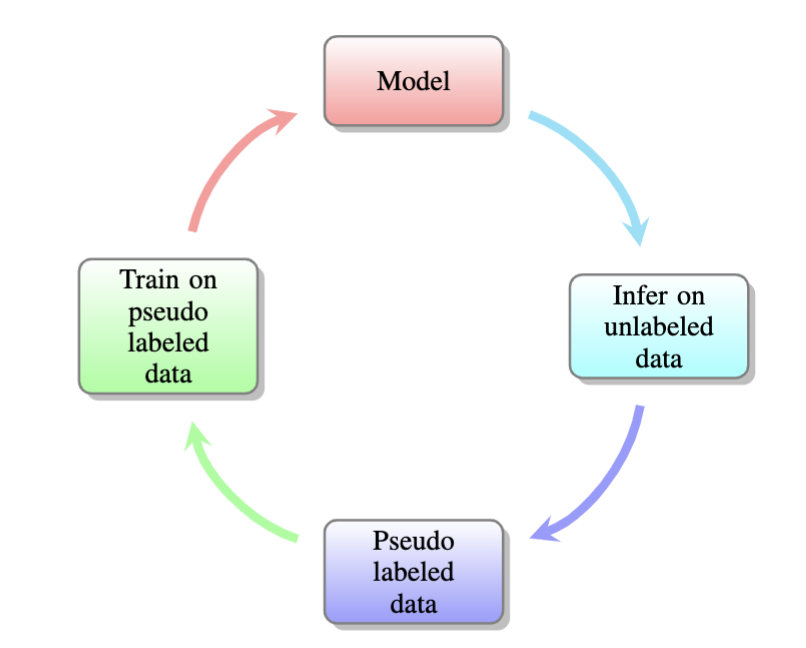
Figure 1: Pseudo label based semi-supervised learning algorithm sketch

1.2 Insight

We provide a novel theoretical analysis of pseudo label based semi-supervised learning algorithm. Under a simple and realistic assumption on the model, we show that when the amount of unlabeled data tends to infinity, the pseudo label based semi-supervised learning algorithm can obtain a model which has the same population error upper bound as supervised learning. More importantly, we give an explicit estimate of the rate of convergence achievable at each iteration. We also give the lower bound on sample complexity to achieve the target convergence rate.

Our assumption about the model is that if we train the model on dataset part of which is randomly labeled, when the proportion of randomly labeled data is low, the model we get can have a lower empirical error on the correct labeled data, and a higher empirical error on the randomly labeled data. This is reasonable and verifiable especially when the model is under-parameterized. It is worth mentioning that even when the DNN models are over-parameterized, the DNN models still tend to fit correct data before mislabeled data.(Liu et al., 2020) and (Arora et al., 2019). We also show the intuition behind the assumption with a toy example. In this toy example, the dataset consists of $(x_{1},y_{1}),(x_{2},y_{2}),(x_{3},y_{3})$ (in color green), and a small part of random mislabeled of them (in color orange). So when we train the DNN models on the dataset as in Figure 2, the model we get will ignore the mislabeled data.

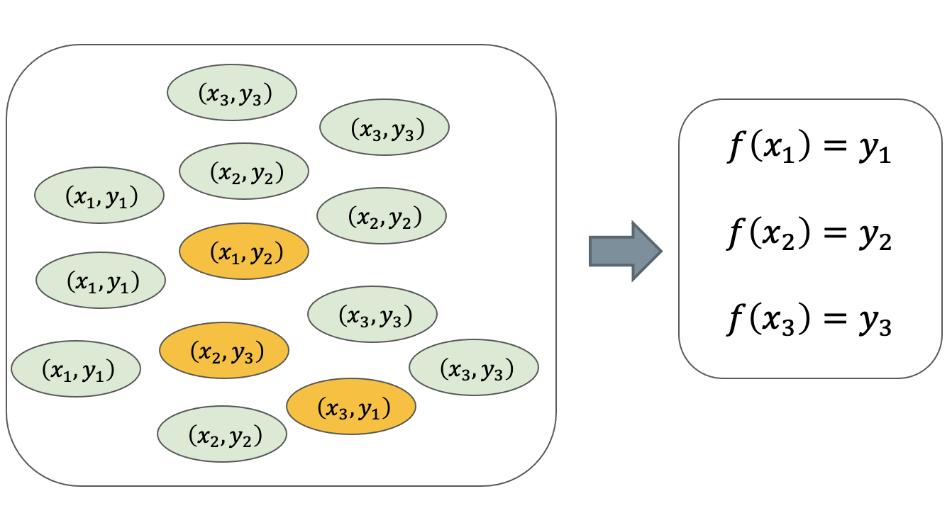
Figure 2: A toy example for our assumption

The same intuition carries to more general cases. If we have a proper initial model and use it to generate pseudo labels on the unlabeled dataset, there will be a small part of the pseudo labels that are wrong-labeled. And if we use the generated pseudo label to train a new model, the model will try to fit the correct labels and will be well-trained since the absolute quantity of the pseudo labels is large based on our assumption. What is more, if the model trained on the pseudo labels is good enough, we can reuse it to generate new pseudo labels on the unlabeled dataset. We hope that the pseudo labels generated by the previous model trained on the pseudo labels will have fewer wrong labels. So we can get a better model from them and the iteration can continue. The process can be continued until no obvious improvement can be obtained. From this perspective, our analysis contributes to understanding the empirical successes of pseudo label-based semi-supervised learning (Laine & Aila, 2016), (Tarvainen & Valpola, 2017), (Lee et al., 2013), (Li et al., 2019), (Graves, 2012), (Chiu et al., 2018) and (Bengio et al., 2015).

In summary, our contributions include:

• We give a theoretical analysis of the pseudo label based algorithm and contribute to understanding the empirical successes of pseudo label based semi-supervised learning.

• We show that, if we have a proper initial model and when the amount of unlabeled data tends to infinity, the algorithm can obtain the model which has the optimal population error upper bound. Here the optimal population error upper bound represents the population error upper bound of the model obtained by supervised learning with all unlabeled data labeled.

• We give an explicit estimate of the rate of convergence achievable at each iteration. Besides, we also give the lower bound on sample complexity to achieve the target convergence rate. Experiments show that our estimates are fairly tight.

2 Related work

2.1 Theory on pseudo label based semi-supervised learning

In the early stage of machine learning, (Sain, 1996) proposes transductive SVM which tried to utilize the unlabeled data. Then (Derbeko et al., 2003) estimates error bounds for transduction learning. Later, (Oymak & Gulcu, 2020) shows pseudo label based semi-supervised learning iterations improve model accuracy even though the model may be plagued by suboptimal fixed points. (Chen et al., 2020) shows that, for a certain class of distributions, entropy minimization on unlabeled target data will reduce the interference of fake features. However, the analysis in (Oymak & Gulcu, 2020) and (Chen et al., 2020) mainly focus on linear models, and DNN models are not analyzed. For DNN models, (Wei et al., 2020) shows that pseudo label based semi-supervised learning method is beneficial to improve the performance of the DNN models, and gives a sample complexity. However, (Wei et al., 2020) did not show that the pseudo label based semi-supervised algorithm can achieve the optimal population error, nor does it estimate the convergence rate of each iteration. Our work successfully addresses these issues.

2.2 Population risk estimation method

There are lots of methods to estimate the population risk of DNN models. One of the most important methods is estimating the upper bound on the population error of DNN models by estimating the complexity of the hypothesis classes (Neyshabur et al., 2015), (Neyshabur et al., 2017), (Ma et al., 2018) and (Weinan et al., 2019). However, this method often is restricted to a specific model and it is hard to use it to create a unified analysis to illustrate the advantage of pseudo label based semi-supervised learning for DNN models. Recently, (Garg et al., 2021) established a method to estimate the population risk of the DNN models via the model performance on randomly labeled data. In the method of (Garg et al., 2021), we will not need to estimate the complexity of the hypothesis classes. So it can help us create a unified analysis for DNN models. And using this method is very convenient to show the benefit of pseudo label based semi-supervised learning since there often will be some mislabeled data in the pseudo labels.

3 Preliminary

3.1 Notation

To be clear, we first show the notation in our paper. We mainly focus on the $k$ classification problem. Using $\mathcal{S}$ represents the labeled data, $n$ represents the amount of dataset $\mathcal{S}$, $\tilde{\mathcal{S}}$ represents the randomly labeled data and $m$ represents the amount of dataset in $\tilde{\mathcal{S}}$. Using $\mathcal{E}_{\mathcal{S}}$ represents 0-1 loss on $\mathcal{S}$, $\mathcal{E}_{\tilde{\mathcal{S}}}$ represents 0-1 loss on $\mathcal{\tilde{S}}$, $\mathcal{E}_{\mathcal{D}}$ represents popluation 0-1 loss.

3.2 Population risk upper bound estimation

As described in Section 2.2, estimating population risk upper bound based on randomly labeled data is convenient to show the benefit of pseudo label based semi-supervised learning since there often will be some mislabeled data in the pseudo labels. What’s more, it can help us to make a unified analysis for DNN models. Now we describe the theorem. This is obviously crucial for our following analysis.

Assumption 3.1.

Let $\hat{f}$ be a model obtained by training with an algorithm $\mathcal{A}$ on a mixture of clean data $S$ and randomly labeled data $\tilde{\mathcal{S}}$. Then with probability $1-\delta$ over the (uniform but without the correct label) mislabeled data $\tilde{\mathcal{S}}_{M}$, we assume that the following condition holds:

$$\mathcal{E}_{\tilde{\mathcal{S}}_{M}}(\widehat{f})\leq\mathcal{E}_{\mathcal{D}^{\prime}}(\widehat{f})+c\sqrt{\frac{\log(1/\delta)}{2m}}$$ (1)

for a fixed constant $c>0$. Where the $\mathcal{E}_{\mathcal{D}^{\prime}}(\widehat{f})$ represents the population loss of $\widehat{f}$ on (uniform but without the correct label) mislabeled data. (Garg et al., 2021)

Theorem 3.2.

Under the Assumption 3.1, then for any $\delta>0$, with probability at least $1-\delta$, we have

$$\mathcal{E}_{\mathcal{D}}(\widehat{f})\leq\mathcal{E}_{\mathcal{S}}(\widehat{f})+(k-1)\left(1-\frac{k}{k-1}\mathcal{E}_{\tilde{\mathcal{S}}}(\widehat{f})\right)\\ +c\sqrt{\frac{\log\left(\frac{4}{\delta}\right)}{2m}}$$ (2)

for some constant $c$ satisfy

$$c\leq\left(2k+\sqrt{k}+\frac{m}{n\sqrt{k}}\right)$$ (3)

Where $m$ represents the amount of dataset $\tilde{\mathcal{S}}$ and $n$ represents the amount of dataset $\mathcal{S}$. (Garg et al., 2021)

Remark 3.3.

The randomly labeled data is not equal to mislabeled data. For $k$ classification problem, the randomly labeled data means for any $x$, its label is uniformly randomly selected from $k$ labels $y_{1},y_{2},y_{3},...,y_{k}$. However, the mislabeled data means for any $x$, its label is uniformly randomly selected from all $k$ labels except its ground truth label. For example, for $x_{1}$, and we suppose its ground truth label is $y_{1}$, then mislabeled data of $x_{1}$ is uniformly randomly selected from $k-1$ labels $y_{2},y_{3},...,y_{k}$.

Remark 3.4.

The Assumption 3.1 holds in almost all scenarios. Since when we train DNN models, they always tend to overfit the training data. In practice, we often need to take steps to prevent overfitting.

3.3 General assumption

As we describe in Section 1.2, our assumption about the model is that if we train the model on the dataset, which parts of it are randomly labeled. When the proportion of randomly labeled data is low, we can obtain models with low empirical error on correctly labeled data and high empirical error on randomly labeled data. Here we give a mathematical formula that describes this assumption in Assumption 3.5.

Assumption 3.5.

$\exists\varepsilon>0,\tilde{\delta}>0,b\geq 0$ if the training dataset $\mathcal{S}\cup\widetilde{\mathcal{S}}$ satisfy

$$\frac{m}{n}\leq\widetilde{\delta}<1$$ (4)

we can get $\hat{f}$ that satisfy

$$\mathcal{E}_{\mathcal{S}}(\hat{f})\leq\varepsilon$$ (5)

$$\mathcal{E}_{\tilde{\mathcal{S}}}(\hat{f})\geq 1-\frac{1+b\varepsilon}{k}$$ (6)

In the following section, we will go further under the condition of Assumption 3.5. Since the $\varepsilon$ and $\tilde{\delta}$ change as the architecture of the model and training data change, exploring how the $\varepsilon$ and $\tilde{\delta}$ change as the architecture of the model and training data change is still an important work, and we think we will do it in the future. And we will discuss under the fixed $\varepsilon$ and $\tilde{\delta}$ in this paper.

In Section 4, we discuss the population risk under the condition that we have $N$ labeled data as the normal training setting. In Section 5, we show that when the amount of unlabeled data tends to infinity, the algorithm can obtain the model which has the optimal population error upper bound. In Section 6, We give an estimation of the convergence rate and the sample complexity.

4 Supervised learning

Firstly, according to Assumption 3.5, we have

$$\frac{m}{n}\leq\widetilde{\delta}<1$$ (7)

and we can give a more relaxed upper bound in Theorem 3.2 to simplify our analysis and notation later.

Theorem 4.1.

Under the Assumption 3.1, then for any $\delta>0$, with probability at least $1-\delta$, we have

$$\mathcal{E}_{\mathcal{D}}(\widehat{f})\leq\mathcal{E}_{\mathcal{S}}(\widehat{f})+(k-1) \left(1-\frac{k}{k-1}\mathcal{E}_{\tilde{\mathcal{S}}}(\widehat{f})\right)$$ (8)

$$+ ak\sqrt{\frac{\log\left(\frac{4}{\delta}\right)}{m}}$$

with constant

$$ak\geq\frac{2k+\sqrt{k}+\frac{\widetilde{\delta}}{\sqrt{k}}}{\sqrt{2}}$$ (9)

and generally, we can have $a=4$. Where $m$ represents the amount of dataset $\tilde{\mathcal{S}}$ and $n$ represents the amount of dataset $\mathcal{S}$ (Garg et al., 2021).

Specifically, if the $\widetilde{\delta}$ in Assumption 3.1 satisify

$${2k+\sqrt{k}+\frac{\widetilde{\delta}}{\sqrt{k}}}<2\sqrt{2}k$$ (10)

We can have a tighter constant $a=2$ in equation 8.

Now, we want to estimate the population risk upper bound of the models normal training on $N$ labeled data by Theorem 4.1. On the one hand, we observe that the second term in Theorem 4.1 is related to performance on random labeled data $\tilde{\mathcal{S}}$. And the third term $ak\sqrt{\frac{\log\left(\frac{4}{\delta}\right)}{m}}$ decreases as $m$ increases. On the other hand, in Assumption 3.5, the $\varepsilon$ show the model performance on both correct labeled data $\mathcal{S}$ and randomly labeled data $\tilde{\mathcal{S}}$. The $\widetilde{\delta}$ limit the upper bound of the amount of randomly labeled data $\tilde{\mathcal{S}}$.

Thus, we can randomly label a small part of $N$ labeled data and we can use the Theorem 4.1 to estimate the population risk and the randomly labeled small part won’t affect much compared with training purely on $N$ labeled data. To satisfy Assumption 3.5, we have

$$\left\{\begin{aligned} &\frac{m}{n}=\tilde{\delta}\\ &m+n=N\end{aligned}\right.$$ (11)

So we have

$$\left\{\begin{aligned} &m=\frac{\tilde{\delta}}{1+\tilde{\delta}}N\\ &n=\frac{1}{1+\tilde{\delta}}N.\end{aligned}\right.$$ (12)

According to Assumption 3.5 and Theorem 4.1, we have $f^{*}$ which satisfy

$$\mathcal{E}_{D}({f}^{*})\leq(1+b)\varepsilon+ak\sqrt{\log\left(\frac{4}{\delta}\right)}\frac{1}{\sqrt{\frac{\tilde{\delta}}{1+\tilde{\delta}}N}}$$ (13)

We denote the population risk upper bound of $f^{*}$ as

$$\mathcal{E}_{D}^{*}:=(1+b)\varepsilon+ak\sqrt{\log\left(\frac{4}{\delta}\right)}\frac{1}{\sqrt{\frac{\tilde{\delta}}{1+\tilde{\delta}}N}}$$ (14)

which reflects the population risk upper bound under the normal setting in which we have $N$ labeled training dataset.

Remark 4.2.

We observe that the $\mathcal{E}_{D}^{*}$ is nearly optimal since it has the error rate order of $O(\frac{1}{\sqrt{N}})$ which is equal to Monte Carlo estimation error rate order. This also implies the reasonableness of our assumption.

5 Effectiveness analysis

In this section, we first discuss the population risk under the condition that we have $N$ unlabeled data and a proper initial model as the pseudo label based algorithm setting. Then we compare the population risk in Section 4 and Section 5 as the amount of (unlabeled) data tends to infinity. We show that when the amount of unlabeled data tends to infinity, the pseudo label based semi-supervised learning algorithm can obtain a model with the same population error upper bound as the model obtained by supervised training in the condition of the amount of labeled data tends to infinity.

5.1 Modified pseudo label based algorithm

In this section we consider the case where we have $N$ unlabeled data and an initial $f_{0}$ as the pseudo label based semi-supervised learning algorithm setting as described in Section 1.1.

We need to generate the pseudo labels by the $f_{0}$ and then train the model by pseudo labels. We denote the $\mathcal{E}_{D}(f_{0})$ as $\gamma_{0}$. Obviously, there are about $(1-\gamma_{0})N$ correct labels and $\gamma_{0}N$ wrong labels in the generated pseudo labels. However, we can not view wrong labels in the generated pseudo labels as random label. A shred of direct evidence is there are no correct labels in the wrong labels in the generated pseudo labels, but there are around $\frac{1}{k}$ correct labels in the random labels. Since both Assumption 3.5 and Theorem 4.1 connect to the model performance in randomly labeled data. A correct way is that we can select a small part of generated pseudo labels and then randomly label them. Then we can use Assumption 3.5 and Theorem 4.1 to estimate the population risk. To be more clear, the modified pseudo label based algorithm, which is used to analyze is shown in Algorithm 2. Step 5 in Algorithm 2, which is mainly modified compared with Algorithm 1, has little effect on pseudo label based algorithm in Algorithm 1 because in practice the $m<<N$ and we will show how to determine $m$ below. But the Algorithm 2 format can help us analyze using the population error tools mentioned above.

Algorithm 2 Modified pseudo label based algorithm

1:  Input: initial model $f_{0}$, $N$ unlabeled data $\mathcal{T}$, test data $\mathcal{T}_{test}$, $\varepsilon,\widetilde{\delta}$ that satisfy Assumption 2, iteration number $I$, $i=0$.

2:  repeat

3:     Estimate the $f_{i}$ population risk $\gamma_{i}$ on $\mathcal{T}_{test}$

4:     Generate pseudo label on $\mathcal{T}$ using $f_{i}$.

5:     Random select proper $m(m<<N)$ part of data from pseudo labeled $\mathcal{T}$ and random labeled them

6:     Update the pseudo labeled $\mathcal{T}$.

7:     Train on pseudo label $\mathcal{T}$.

8:     $i\leftarrow i+1$

9:  until $i=I$

9:  Model $f_{I}$

5.2 Effectiveness of the pseudo label based semi-supervised learning algorithm

To satisfy Assumption 3.5, the amount of data selected to random label $m$ in Algorithm 2 has the following restriction.

$$\frac{m+\gamma_{0}(N-m)}{(1-\gamma_{0})(N-m)}\leq\widetilde{\delta}$$ (15)

So, we have

$$m\leq\frac{\widetilde{\delta}(1-\gamma_{0})-\gamma_{0}}{(1+\widetilde{\delta})(1-\gamma_{0})}N$$ (16)

$$\gamma_{0}\leq\frac{\widetilde{\delta}}{1+\tilde{\delta}}$$ (17)

The equation 16 shows that we can select at most $\frac{\widetilde{\delta}(1-\gamma_{0})-\gamma_{0}}{(1+\widetilde{\delta})(1-\gamma_{0})}N$ data from $N$ generated pseudo labels then random labeled them when the $\gamma_{0}$ satisfy equation 17. According to Assumption 3.5 and Theorem 4.1, we can get $f_{1}$ and with at least $(1-\delta)$ probability we have

$$\mathcal{E}_{D}({f}_{1})\leq(1+b)\varepsilon+ak\sqrt{\log\left(\frac{4}{\delta}\right)}\sqrt{\frac{(1+\widetilde{\delta})(1-\gamma_{0})}{\tilde{\delta}(1-\gamma_{0})-\gamma_{0}}}\frac{1}{\sqrt{N}}$$ (18)

Compare $\mathcal{E}_{D}({f}_{1})$ with $\mathcal{E}_{D}^{*}:=(1+b)\varepsilon+ak\sqrt{\log\left(\frac{4}{\delta}\right)}\frac{1}{\sqrt{\frac{\tilde{\delta}}{1+\tilde{\delta}}N}}$ in equation 14, we can easily show that

$$\lim_{N\to+\infty}\frac{\mathcal{E}_{D}(f_{1})}{\mathcal{E}_{D}^{*}}\leq 1.$$ (19)

In summary, we have

Theorem 5.1.

Under the condition of Assumption 3.5, for fixed $\varepsilon$, $\widetilde{\delta}$ and $\forall\delta\in(0,1)$, if we have $f_{0}$ with $\gamma_{0}:=\mathcal{E}_{D}(f_{0})<\frac{\widetilde{\delta}}{1+\tilde{\delta}}$ and $N$ unlabeled data, then by Algorithm 2, with at least $(1-\delta)$ probability, we can get $f_{1}$ that satisfies

$$\lim_{N\to+\infty}\frac{\mathcal{E}_{D}(f_{1})}{\mathcal{E}_{D}^{*}}=1.$$ (20)

This result implies that if we have a proper $f_{0}$ and the amount of input unlabeled data tends to be infinite, pseudo label based semi-supervised algorithm can obtain a model in which the population error upper bound is optimal which means it is equal to the population error upper bound of the model trained in the condition of amount of labeled data tends to infinite. Further, this can be achieved even in ONE iteration. This actually shows the power of the pseudo label based semi-supervised algorithm.

6 Sample complexity and convergence rate

In this section, we give an explicit estimate of the rate of convergence achievable at each iteration. We also give the lower bound on sample complexity to achieve the target convergence rate.

As analysis in Section 5.1, if we use an initial model with population risk $\gamma_{0}$, the population risk uppper bound of $f_{1}$ by Algorithm 2 with at least $(1-\delta)$ probability we have

$$\mathcal{E}_{D}({f}_{1})\leq(1+b)\varepsilon+ak\sqrt{\log\left(\frac{4}{\delta}\right)}\sqrt{\frac{(1+\widetilde{\delta})(1-\gamma_{0})}{\tilde{\delta}(1-\gamma_{0})-\gamma_{0}}}\frac{1}{\sqrt{N}}$$ (21)

If the model $f_{1}$ trained on the pseudo labels is good enough, we can reuse it to generate new pseudo labels on the unlabeled dataset and then obtain the new model $f_{2}$. We hope that the pseudo labels generated by the $f_{1}$ model trained on the pseudo labels will have fewer wrong labels than $f_{0}$. So we can get a better model from them and the iteration can continue. Here, we are interested in if the population risk upper bound can approximate the ${\mathcal{E}_{D}^{*}}$ and how fast it is. So we should care if we can achieve

$$\frac{{\mathcal{E}_{D}(f_{i+1})}-\mathcal{E}_{D}^{*}}{{\mathcal{E}_{D}(f_{i})}-\mathcal{E}_{D}^{*}}\triangleq p\leq p^{*}$$ (22)

where $f_{i},f_{i+1}$ denote the output of $i$th and $i+1$th iteration in Algorithm 2, $p^{*}$ is the target convergence rate in $(0,1)$. We denote the population risk of $f_{i}$ as $\gamma_{i}$. Then according to the analysis in Section 5.1, if

$$\gamma_{i}\leq\frac{\widetilde{\delta}}{1+\tilde{\delta}}$$ (23)

we can get $f_{i+1}$ that with at least $(1-\delta)$ probability we have

$$\begin{split}\mathcal{E}_{D}({f}_{i+1})&\leq(1+b)\varepsilon+ak\sqrt{\log\left(\frac{4}{\delta}\right)}\sqrt{\frac{(1+\widetilde{\delta})(1-\gamma_{i})}{\tilde{\delta}(1-\gamma_{i})-\gamma_{i}}}\\ &\cdot\frac{1}{\sqrt{N}}\triangleq upper(f_{i+1})\end{split}$$ (24)

The straightforward point is that we have

$$p\triangleq\frac{{\mathcal{E}_{D}(f_{i+1})}-\mathcal{E}_{D}^{*}}{{\mathcal{E}_{D}(f_{i})}-\mathcal{E}_{D}^{*}}\leq\frac{upper(f_{i+1})-\mathcal{E}_{D}^{*}}{{\mathcal{E}_{D}(f_{i})}-\mathcal{E}_{D}^{*}}\triangleq\widetilde{p}$$ (25)

So we can consider equation 22 by considering

$$\widetilde{p}\leq p^{*}$$ (26)

Without loss of generality, we can further assume the $\gamma_{i}=\mathcal{E}_{D}(f_{i})$ satisfies

$$\mathcal{E}_{D}^{*}+c_{1}\leq\gamma_{i}\leq\mathcal{E}_{D}^{*}+c_{2}$$ (27)

where $c_{1}$ and $c_{2}$ are two positive constant and $c_{1}$ can be arbitrarily small.

Then solve the equation 26 we can get

$$N\geq\left(\frac{ak}{p^{*}c_{1}}\right)^{2}\left[\sqrt{\frac{\tilde{\delta}+1}{\tilde{\delta}-\frac{\mathcal{E}_{D}^{*}+c_{2}}{1-\mathcal{E}_{D}^{*}-c_{2}}}}-\sqrt{\frac{\tilde{\delta}+1}{\tilde{\delta}}}\right]^{2}\log\left(\frac{4}{\delta}\right)$$ (28)

Hence, we have

Theorem 6.1 (Sample Complexity Estimation).

Under the condition of Assumption 3.5, for fixed $\varepsilon$, $\widetilde{\delta}$ satisfy Assumption 3.5 and $\forall\delta,c_{1},c_{2},p^{*}\in(0,1)$ and $c_{1}\leq c_{2}$, we define $\mathcal{E}_{D}^{*}$ as equation 14. If the number of unlabeled data $N$ satisfy

$$N\geq\left(\frac{ak}{p^{*}c_{1}}\right)^{2}\left[\sqrt{\frac{\tilde{\delta}+1}{\tilde{\delta}-\frac{\mathcal{E}_{D}^{*}+c_{2}}{1-\mathcal{E}_{D}^{*}-c_{2}}}}-\sqrt{\frac{\tilde{\delta}+1}{\tilde{\delta}}}\right]^{2}\log\left(\frac{4}{\delta}\right)$$ (29)

and

$$\mathcal{E}_{D}^{*}+c_{1}\leq\mathcal{E}_{D}(f_{i})\leq\mathcal{E}_{D}^{*}+c_{2}$$ (30)

$$\mathcal{E}_{D}(f_{i})\leq\frac{\tilde{\delta}}{1+\tilde{\delta}}$$ (31)

then with at least $(1-\delta)^{2}$ probability we have

$$p\triangleq\frac{{\mathcal{E}_{D}(f_{i+1})}-\mathcal{E}_{D}^{*}}{{\mathcal{E}_{D}(f_{i})}-\mathcal{E}_{D}^{*}}\leq p^{*}$$ (32)

where $f_{i},f_{i+1}$ denote the output of $i$th and $i+1$th iteration in Algorithm 2.

Since $c_{1}$ could be arbitrarily small, this result indeed shows that the population risk by pseudo label based algorithm can approximate to the normally trained population risk ${\mathcal{E}_{D}^{*}}$ as the pseudo label based algorithm iteration progresses.

And note that for a fix $N$ and $p^{*}$, the right-hand term of equation 29 increases as the $c_{1}$ decreases and as $c_{2}$ increases. Hence for $f_{i}$, the most loose condition of equation 29 will reach at $c_{1}=c_{2}=\mathcal{E}_{D}(f_{i})-\mathcal{E}_{D}^{*}$. So we have,

Corollary 6.2.

Under the condition of Assumption 3.5, for fixed $\varepsilon$, $\widetilde{\delta}$ satisfy Assumption 3.5 and $\forall\delta,p^{*}\in(0,1)$, we define $\mathcal{E}_{D}^{*}$ as equation 14. If the number of unlabeled data $N$ satisfy

$$\begin{split}N\geq&\left(\frac{ak}{p^{*}(\mathcal{E}_{D}(f_{i})-\mathcal{E}_{D}^{*})}\right)^{2}\left[\sqrt{\frac{\tilde{\delta}+1}{\tilde{\delta}-\frac{\mathcal{E}_{D}(f_{i})}{1-\mathcal{E}_{D}(f_{i})}}}-\sqrt{\frac{\tilde{\delta}+1}{\tilde{\delta}}}\right]^{2}\\ &\cdot\log\left(\frac{4}{\delta}\right)\end{split}$$ (33)

and

$$\mathcal{E}_{D}(f_{i})\leq\frac{\tilde{\delta}}{1+\tilde{\delta}}$$ (34)

then with at least $(1-\delta)^{2}$ probability we have

$$p\triangleq\frac{{\mathcal{E}_{D}(f_{i+1})}-\mathcal{E}_{D}^{*}}{{\mathcal{E}_{D}(f_{i})}-\mathcal{E}_{D}^{*}}\leq p^{*}$$ (35)

where $f_{i},f_{i+1}$ denote the output of $i$th and $i+1$th iteration in Algorithm 2.

More importantly, we can estimate the convergence rate by equation 24 and equation 25 when we have a fixed number of samples $N$.

Theorem 6.3 (Convergence Rate Estimation).

Under the condition of Assumption 3.5, for fixed $\varepsilon$, $\widetilde{\delta}$ satisfy Assumption 3.5 and $\forall\delta\in(0,1)$, we define $\mathcal{E}_{D}^{*}$ as equation 14. If we have $N$ samples, and

$$\mathcal{E}_{D}(f_{i})\leq\frac{\tilde{\delta}}{1+\tilde{\delta}}$$ (36)

then with at least $O(1-\delta)^{2}$ probability we have

$$\begin{split}p\leq&\frac{(ak)}{(\mathcal{E}_{D}(f_{i})-\mathcal{E}_{D}^{*})\sqrt{N}}\left[\sqrt{\frac{\tilde{\delta}+1}{\tilde{\delta}-\frac{\mathcal{E}_{D}(f_{i})}{1-\mathcal{E}_{D}(f_{i})}}}-\sqrt{\frac{\tilde{\delta}+1}{\tilde{\delta}}}\right]\\ &\cdot\sqrt{\log\left(\frac{4}{\delta}\right)}\end{split}$$ (37)

Here $p\triangleq\frac{{\mathcal{E}_{D}(f_{i+1})}-\mathcal{E}_{D}^{*}}{{\mathcal{E}_{D}(f_{i})}-\mathcal{E}_{D}^{*}}$ as above and $f_{i},f_{i+1}$ denote the output of $i$th and $i+1$th iteration in Algorithm 2.

7 Experiment

7.1 Dataset

We conduct experiments on the CIFAR-10 dataset and FashionMnist dataset respectively. Both the CIFAR-10 dataset and the FashionMnist dataset are widely used datasets in machine learning research. For CIFAR-10 dataset, it contains 60,000 32x32 color images from 10 different classes. The training split has 50,000 32x32 color images and the test split has 10,000 32x32 color images. For FashionMnist dataset, it covers a total of 70,000 28x28 grayscale images from 10 categories, of which 60,000 are used as training sets and 10,000 are used as test sets.

In order to ensure the sample volume requirements, we expanded the sample size of the training set from 50,000 to 200,000 (4 times) by random cropping, etc for the CIFAR-10 dataset and expanded the sample size of the training set from 60,000 to 180,000 (3 times) by random cropping, etc for FashionMnist dataset. Besides, we construct a binary classification problem instead of an official 10 classification problem by combining five classes in the dataset into one class for both experiments on two datasets.

7.2 Model

We use a 10 layers resnet (He et al., 2016) with a 3x3 kernel size for both experiments on two datasets. Model structure and hyperparameters are shown in Figure 3. For optimization, we use the SGD optimizer with an initial 0.1 learning rate and a multistep learning rate scheduler.

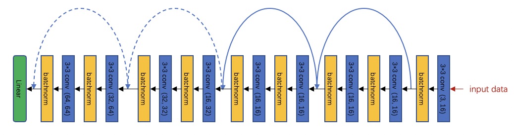
Figure 3: Model architecture

7.3 Experiment on CIFAR-10 dataset

We show $\tilde{\delta}=0.3,\varepsilon=0.0465,b=0.906$ satisfy Assumption 3.5 in Appendix A.1. Now we test the convergence rate in Theorem 6.3. In the experiment we have the number of classes $k=2$, hence equation 10 is correct and we can select $a=2$. So according to the equation 14, we can calculate the $\mathcal{E}_{D}^{*}:=(1+b)\varepsilon+ak\sqrt{\log\left(\frac{4}{\delta}\right)}\frac{1}{\sqrt{\frac{\tilde{\delta}}{1+\tilde{\delta}}N}}$ with different probability tolerance $1-\delta$. The results are shown in Table 1.

$\delta$	0.025	0.05	0.1
$\mathcal{E}_{D}^{*}$	0.131	0.128	0.124

Table 1: The $\mathcal{E}_{D}^{*}$ with different $\delta$

For $f_{i}$ ($i=0$ here), we get the $f_{i}$ by training the model in subsection 7.2 on 10000 images randomly sampled on raw CIFAR-10 dataset and achieve a 0.183 test error rate. The error rate on dataset test split via epoch is shown in Appendix A.2.

Finally, we can calculate the convergence rate according to equation 37 with different probability tolerance $(1-\delta)^{2}$. And then we can get the $\mathcal{E}_{D}(f_{i+1})$ upper bound with different probability tolerance $(1-\delta)^{2}$ by $p\triangleq\frac{{\mathcal{E}_{D}(f_{i+1})}-\mathcal{E}_{D}^{*}}{{\mathcal{E}_{D}(f_{i})}-\mathcal{E}_{D}^{*}}$. Experiment results are shown in Figure 4. It can be seen that the bounds we give are quite tight.

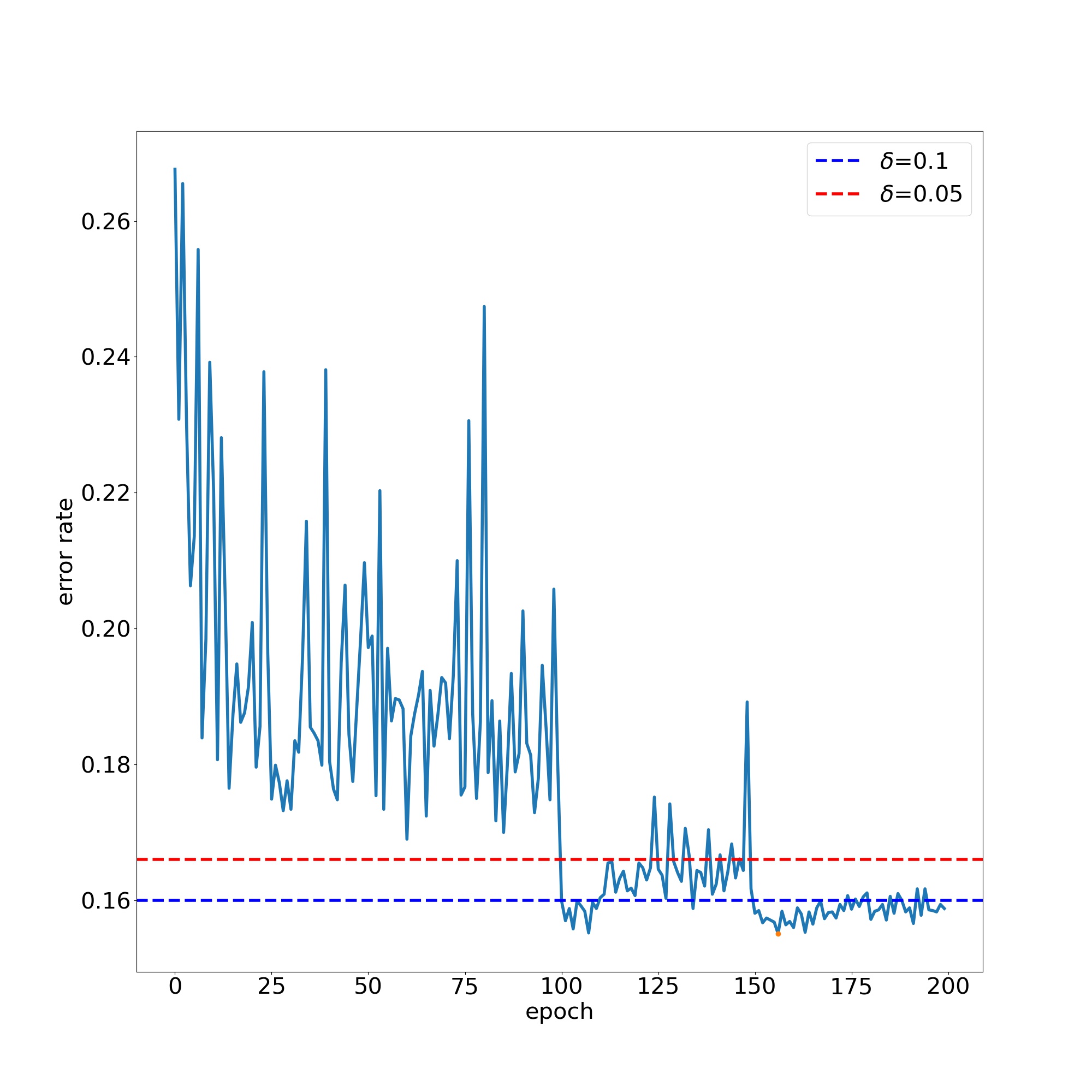
Figure 4: The $\mathcal{E}_{D}(f_{i+1})$ upper bound with different probability tolerance $(1-\delta)^{2}$: $\delta=0.05$ (red line) and $\delta=0.1$ (blue line). Hence the upper bound of convergence rate in Theorem 6.3 is fairly tight.

7.4 Experiment on FashionMnist dataset

We show $\tilde{\delta}=0.35,\varepsilon=0.024,b=0.77$ satisfy Assumption 3.5 in Appendix B.1. Now we test the convergence rate in Theorem 6.3. And in the experiment we have the number of classes $k=2$, hence equation 10 is correct and we can select $a=2$. So according to the equation 14, we can calculate the $\mathcal{E}_{D}^{*}:=(1+b)\varepsilon+ak\sqrt{\log\left(\frac{4}{\delta}\right)}\frac{1}{\sqrt{\frac{\tilde{\delta}}{1+\tilde{\delta}}N}}$ with different probability tolerance $1-\delta$. The resultas are shown in Table 2

$\delta$	0.025	0.05	0.1
$\mathcal{E}_{D}^{*}$	0.084	0.081	0.078

Table 2: The $\mathcal{E}_{D}^{*}$ in different $\delta$ selection

For $f_{i}$ ($i=0$ here), we get the $f_{i}$ by training the model in subsection 7.2 on 1200 images randomly sampled on the raw training set of FashionMnist dataset and achieve a 0.095 test error rate. The error rate on dataset test split via epoch is shown in Appendix B.2.

Finally, we can calculate the convergence rate according to equation 37 with different probability tolerance $(1-\delta)^{2}$. And then we can get the $\mathcal{E}_{D}(f_{i+1})$ upper bound with different probability tolerance $(1-\delta)^{2}$ by $p\triangleq\frac{{\mathcal{E}_{D}(f_{i+1})}-\mathcal{E}_{D}^{*}}{{\mathcal{E}_{D}(f_{i})}-\mathcal{E}_{D}^{*}}$. Experiment results are shown in Figure 5.

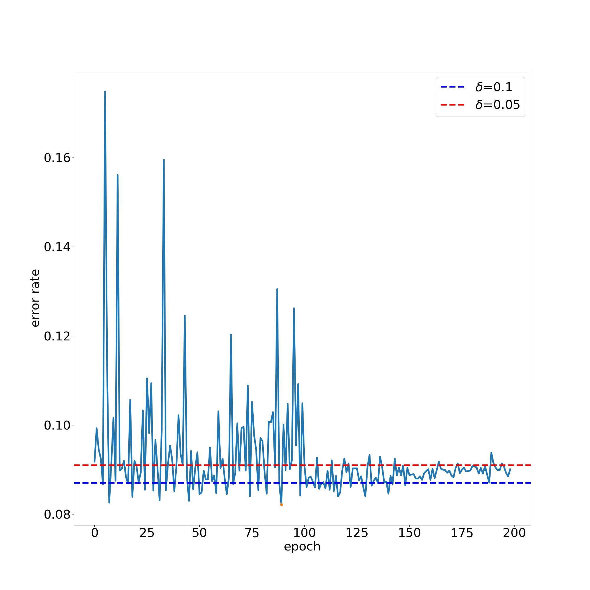
Figure 5: The $\mathcal{E}_{D}(f_{i+1})$ upper bound with different probability tolerance $(1-\delta)^{2}$: $\delta=0.1$ (blue line) and $\delta=0.05$ (red line). Hence the upper bound of convergence rate in Theorem 6.3 is fairly tight.

8 Conclution and future work

We conduct a theoretical analysis of pseudo label based algorithm. We analyzed its effectiveness and we give an explicit estimate of the rate of convergence and sample complexity. Our Assumption 3.5 is important to our analysis and we have explained the reasonableness of the assumption in Section 1.2. But how the $\varepsilon$ and $\tilde{\delta}$ change as the architecture of the model and training data change is still mysterious to us, and we will explore it in the future. We hope that our analysis helps to understand the empirical success and reveal the potential of pseudo label based semi-supervised learning algorithm, and facilitate its application in wider scenarios.

Appendix A Experiment on CIFAR-10 dataset

A.1 Assumption test

We should determine the appropriate $\varepsilon,\tilde{\delta},b$ in the Assumption 3.5. We conduct this by selecting a proper $\tilde{\delta}$ and then determine the proper $\varepsilon$ and $b$ according to the experiment results under the $\tilde{\delta}$. Here, we select $\tilde{\delta}=0.3$ and hence $200,000\times\tilde{\delta}=60,000$ are random labeled. As description in Assumption 3.5, we train on $\mathcal{S}\cup\widetilde{\mathcal{S}}$ and the error rate on $\mathcal{S}$ and $\widetilde{\mathcal{S}}$ are shown in Figure 6. We first select the $\varepsilon=0.0465$ according to the error rate on $\mathcal{S}$ because $\varepsilon=0.0465$ is relatively small compared with the model error rate and can lead to a tight upper bound. Then we select $b=0.906$ to make sure $1-\frac{1+b\varepsilon}{k}$ is a lower bound of the error rate on $\tilde{\mathcal{S}}$. The red line in the right picture of Figure 6 is $1-\frac{1+b\varepsilon}{k}$ with $b=0.906,\varepsilon=0.0465,k=2$ and we see that $b=0.906$ is a fairly good choice. In summary, we select $\tilde{\delta}=0.3,\varepsilon=0.0465,b=0.906$ which satisfy the Assumption 3.5.

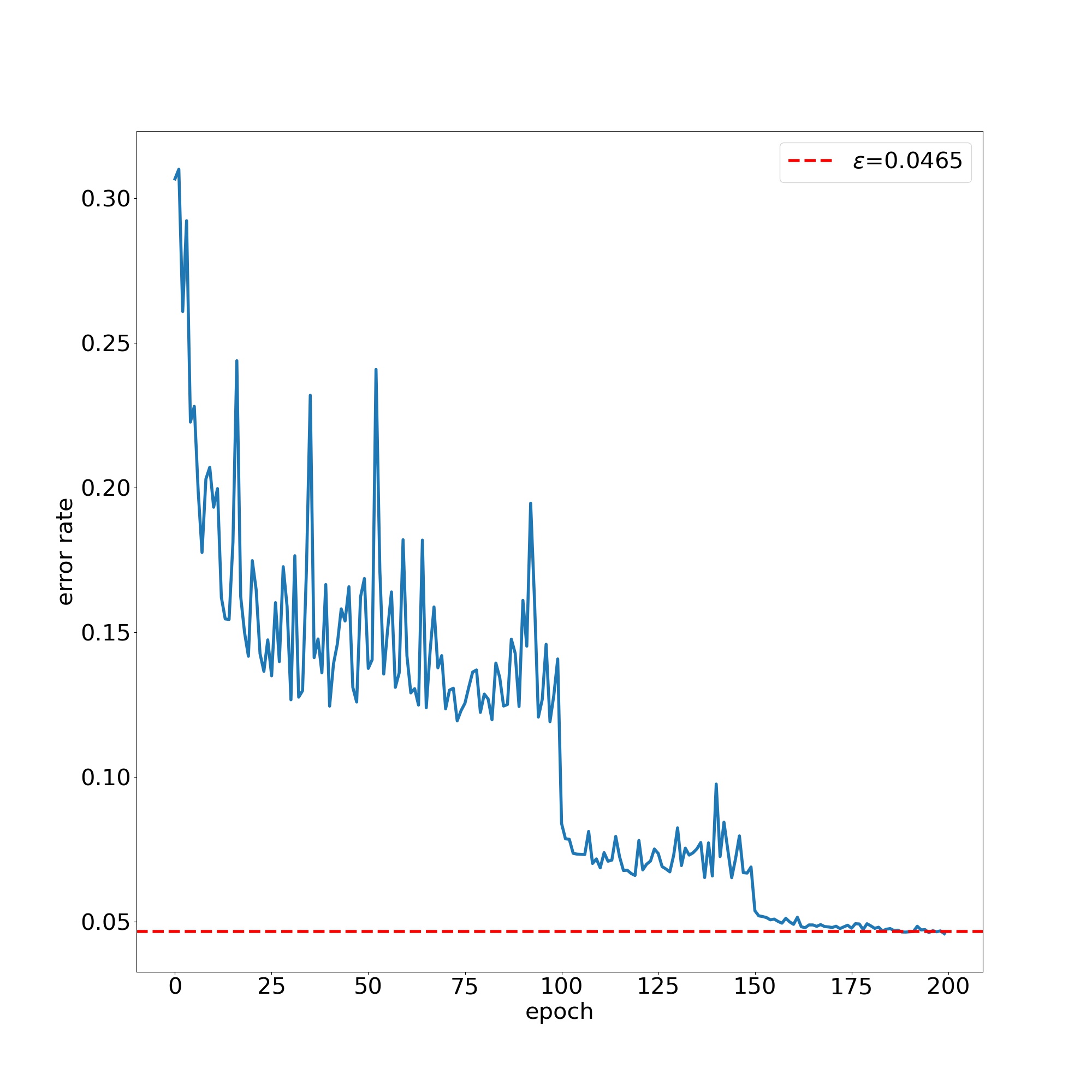
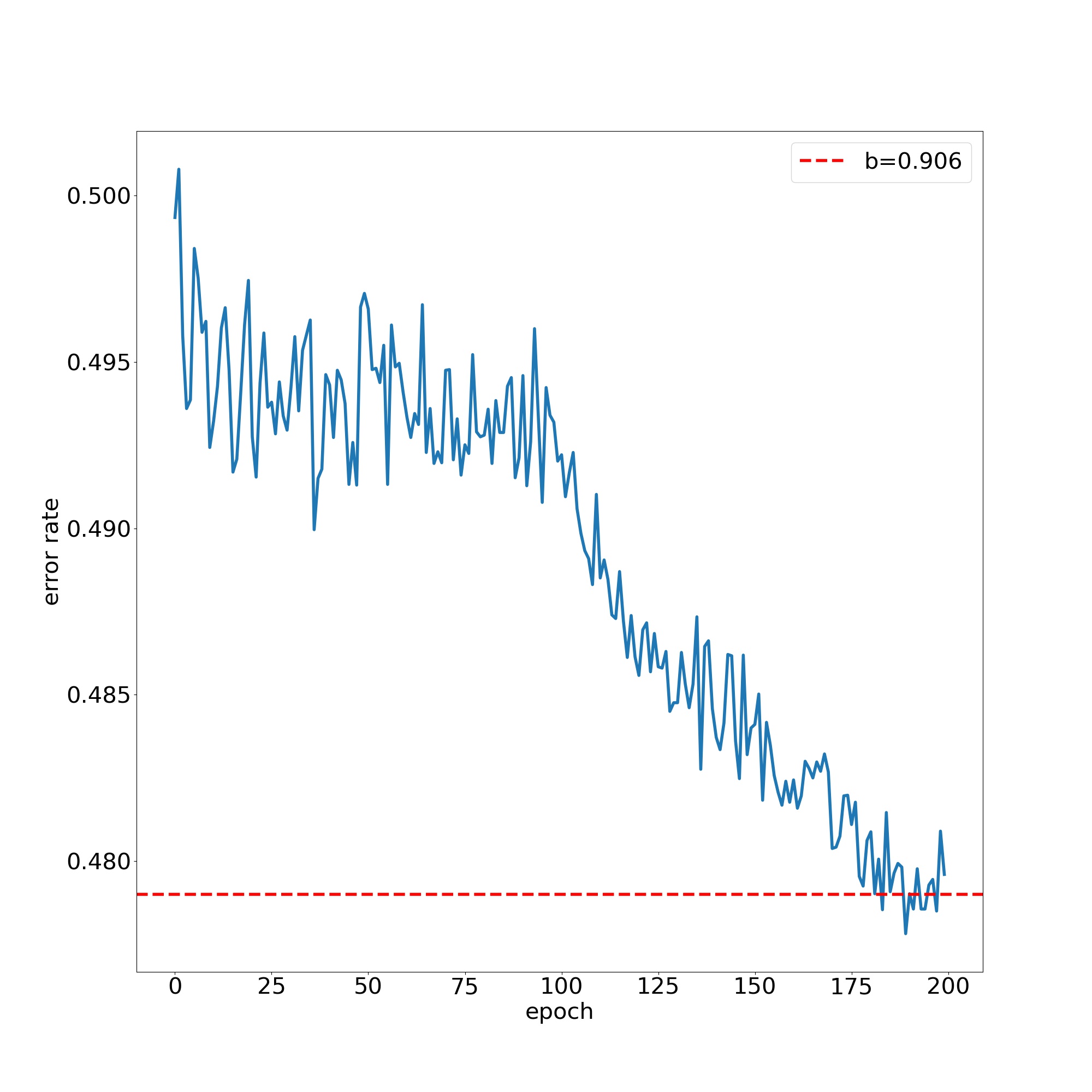
Figure 6: Error rate on correct labeled data $\mathcal{S}$ (left) and random labeled data $\widetilde{\mathcal{S}}$ (right). We can see that the $\varepsilon=0.0465,b=0.906$ is a good choice for Assumption 3.5.

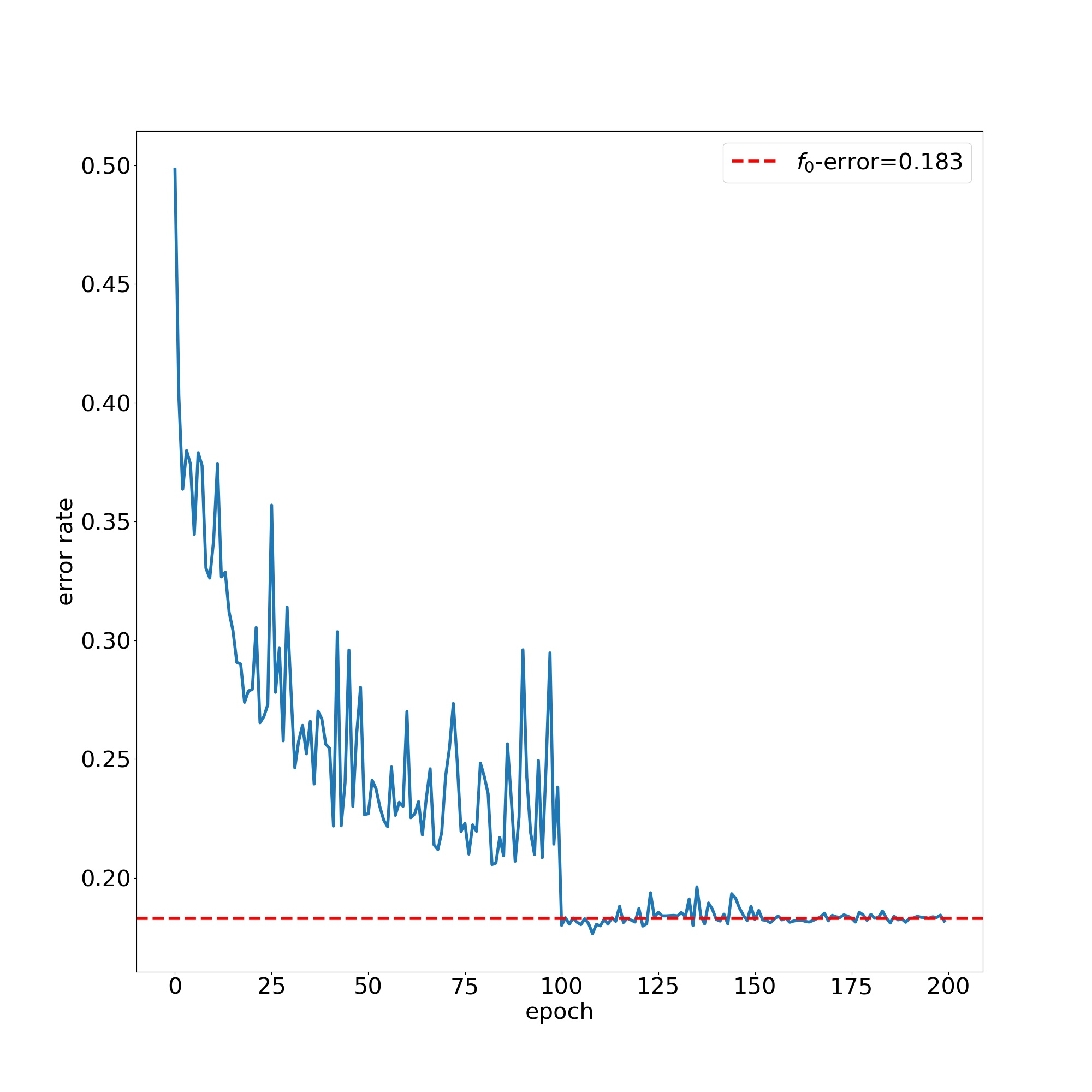
Figure 7: The test error rate of $f_{i}$ via epoch and we can see that the $f_{i}$ can achieve a 0.183 test error rate.

A.2 Model $f_{i}$

For $f_{i}$ ($i=0$ here), we get the $f_{i}$ by training the model in subsection 7.2 on 10000 images randomly sampled on raw CIFAR-10 dataset and achieve a 0.183 test error rate. The error rate on dataset test split via epoch is shown in Figure 7.

Appendix B Experiment on FashionMnist dataset

B.1 Assumption test

Similar to Section 7.3, firstly, we should determine the appropriate $\varepsilon,\tilde{\delta},b$ in the Assumption 3.5. We conduct this by selecting a proper $\tilde{\delta}$ and then determine the proper $\varepsilon$ and $b$ according to the experiment results under the $\tilde{\delta}$. Here, we select $\tilde{\delta}=0.35$ and hence $180,000\times\tilde{\delta}=63,000$ are random labeled. As description in Assumption 3.5, we train on $\mathcal{S}\cup\widetilde{\mathcal{S}}$ and the error rate on $\mathcal{S}$ and $\widetilde{\mathcal{S}}$ are shown in Figure 8. We first select the $\varepsilon=0.024$ according to the error rate on $\mathcal{S}$ because $\varepsilon=0.024$ is relatively small compared with the model error rate on the $\mathcal{S}$ and can lead to a fairly tight upper bound. Then we select $b=0.77$ to make sure $1-\frac{1+b\varepsilon}{k}$ is a lower bound of the error rate on $\tilde{\mathcal{S}}$. The red line in the right picture of Figure 8 is $1-\frac{1+b\varepsilon}{k}$ with $b=0.77,\varepsilon=0.024,k=2$ and we see that $b=0.77$ is a fairly good choice. In summary, we select $\tilde{\delta}=0.35,\varepsilon=0.024,b=0.77$ which satisfy the Assumption 3.5.

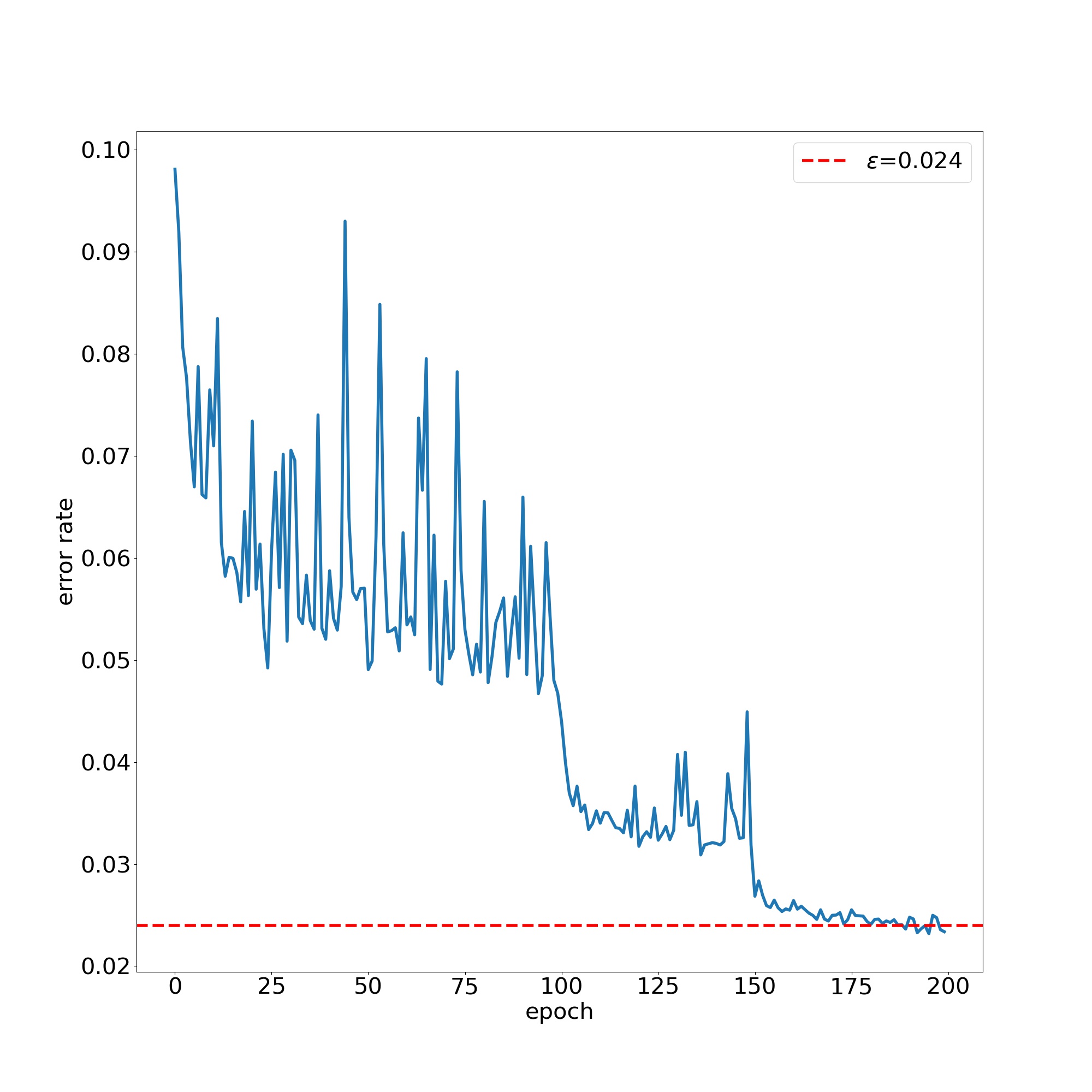
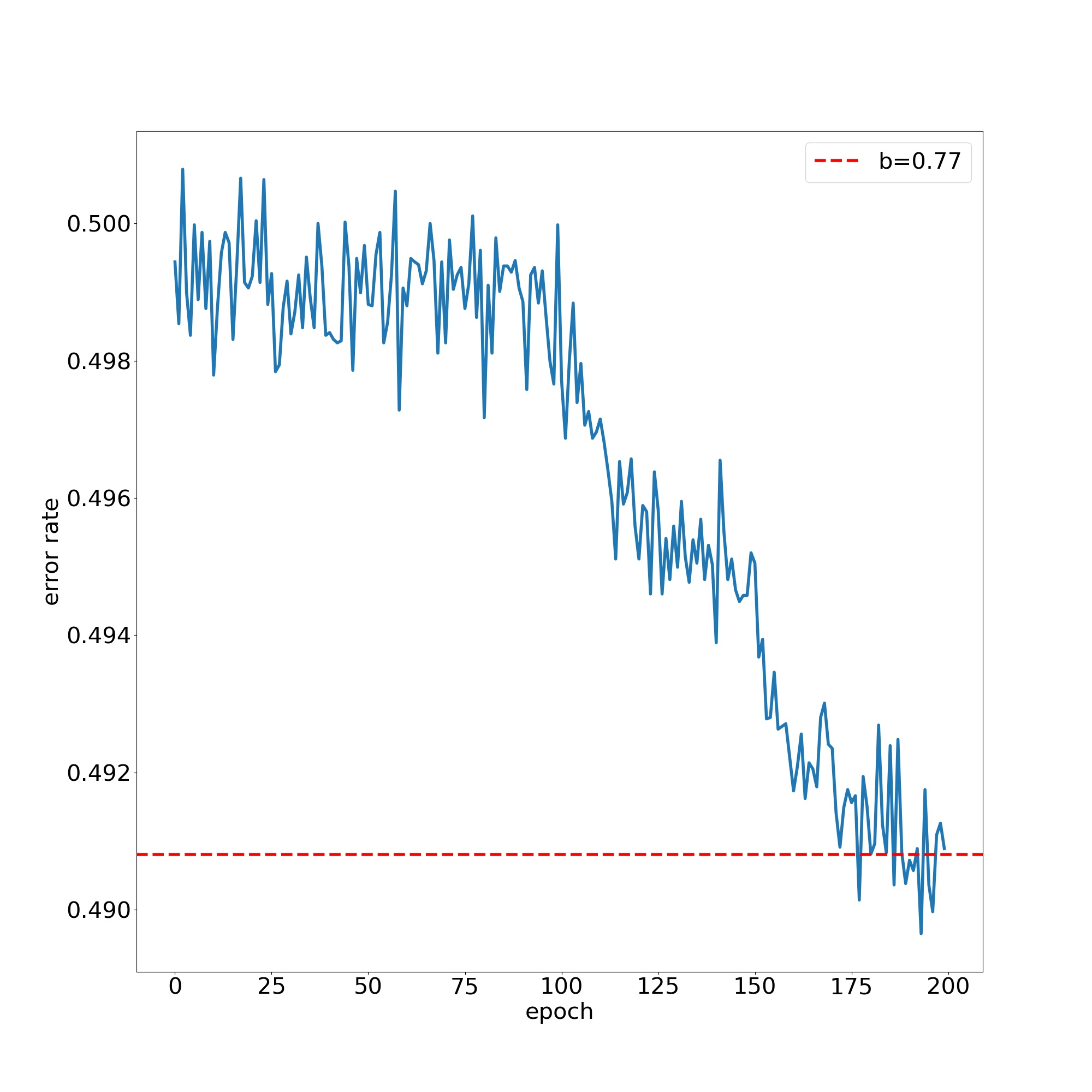
Figure 8: Error rate on correct labeled data $\mathcal{S}$ (left) and random labeled data $\widetilde{\mathcal{S}}$ (right). We can see that the $\varepsilon=0.024,b=0.77$ is a good choice for Assumption 3.5.

B.2 Model $f_{i}$

For $f_{i}$ ($i=0$ here), we get the $f_{i}$ by training the model in subsection 7.2 on 1200 images randomly sampled on the raw training set of FashionMnist dataset and achieve a 0.095 test error rate. The error rate on dataset test split via epoch is shown in Figure 9.

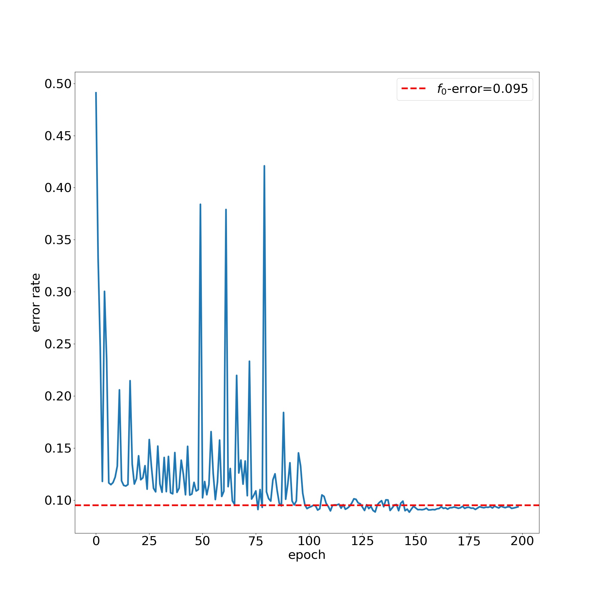
Figure 9: The test error rate of $f_{i}$ via epoch and we can see that the $f_{i}$ can achieve a 0.095 test error rate.

References

- Arora et al. (2019) Arora, S., Du, S., Hu, W., Li, Z., and Wang, R. Fine-grained analysis of optimization and generalization for overparameterized two-layer neural networks. In International Conference on Machine Learning, pp. 322–332. PMLR, 2019.
- Baevski et al. (2020) Baevski, A., Zhou, Y., Mohamed, A., and Auli, M. wav2vec 2.0: A framework for self-supervised learning of speech representations. Advances in Neural Information Processing Systems, 33:12449–12460, 2020.
- Bengio et al. (2015) Bengio, S., Vinyals, O., Jaitly, N., and Shazeer, N. Scheduled sampling for sequence prediction with recurrent neural networks. Advances in neural information processing systems, 28, 2015.
- Brown et al. (2020) Brown, T., Mann, B., Ryder, N., Subbiah, M., Kaplan, J. D., Dhariwal, P., Neelakantan, A., Shyam, P., Sastry, G., Askell, A., et al. Language models are few-shot learners. Advances in neural information processing systems, 33:1877–1901, 2020.
- Chen et al. (2020) Chen, Y., Wei, C., Kumar, A., and Ma, T. Self-training avoids using spurious features under domain shift. Advances in Neural Information Processing Systems, 33:21061–21071, 2020.
- Chiu et al. (2018) Chiu, C.-C., Sainath, T. N., Wu, Y., Prabhavalkar, R., Nguyen, P., Chen, Z., Kannan, A., Weiss, R. J., Rao, K., Gonina, E., et al. State-of-the-art speech recognition with sequence-to-sequence models. In 2018 IEEE International Conference on Acoustics, Speech and Signal Processing (ICASSP), pp. 4774–4778. IEEE, 2018.
- Derbeko et al. (2003) Derbeko, P., El-Yaniv, R., and Meir, R. Error bounds for transductive learning via compression and clustering. Advances in Neural Information Processing Systems, 16, 2003.
- Devlin et al. (2018) Devlin, J., Chang, M.-W., Lee, K., and Toutanova, K. Bert: Pre-training of deep bidirectional transformers for language understanding. arXiv preprint arXiv:1810.04805, 2018.
- Garg et al. (2021) Garg, S., Balakrishnan, S., Kolter, Z., and Lipton, Z. Ratt: Leveraging unlabeled data to guarantee generalization. In International Conference on Machine Learning, pp. 3598–3609. PMLR, 2021.
- Grandvalet & Bengio (2004) Grandvalet, Y. and Bengio, Y. Semi-supervised learning by entropy minimization. Advances in neural information processing systems, 17, 2004.
- Graves (2012) Graves, A. Sequence transduction with recurrent neural networks. arXiv preprint arXiv:1211.3711, 2012.
- He et al. (2016) He, K., Zhang, X., Ren, S., and Sun, J. Deep residual learning for image recognition. In Proceedings of the IEEE conference on computer vision and pattern recognition, pp. 770–778, 2016.
- Kingma et al. (2014) Kingma, D. P., Mohamed, S., Jimenez Rezende, D., and Welling, M. Semi-supervised learning with deep generative models. Advances in neural information processing systems, 27, 2014.
- Laine & Aila (2016) Laine, S. and Aila, T. Temporal ensembling for semi-supervised learning. arXiv preprint arXiv:1610.02242, 2016.
- Lee et al. (2013) Lee, D.-H. et al. Pseudo-label: The simple and efficient semi-supervised learning method for deep neural networks. In Workshop on challenges in representation learning, ICML, volume 3, pp. 896, 2013.
- Li et al. (2019) Li, J., Wang, X., Li, Y., et al. The speechtransformer for large-scale mandarin chinese speech recognition. In ICASSP 2019-2019 IEEE International Conference on Acoustics, Speech and Signal Processing (ICASSP), pp. 7095–7099. IEEE, 2019.
- Liu et al. (2020) Liu, S., Niles-Weed, J., Razavian, N., and Fernandez-Granda, C. Early-learning regularization prevents memorization of noisy labels. Advances in neural information processing systems, 33:20331–20342, 2020.
- Liu et al. (2019) Liu, Y., Ott, M., Goyal, N., Du, J., Joshi, M., Chen, D., Levy, O., Lewis, M., Zettlemoyer, L., and Stoyanov, V. Roberta: A robustly optimized bert pretraining approach. arXiv preprint arXiv:1907.11692, 2019.
- Ma et al. (2018) Ma, C., Wu, L., et al. A priori estimates of the population risk for two-layer neural networks. arXiv preprint arXiv:1810.06397, 2018.
- Neyshabur et al. (2015) Neyshabur, B., Tomioka, R., and Srebro, N. Norm-based capacity control in neural networks. In Conference on Learning Theory, pp. 1376–1401. PMLR, 2015.
- Neyshabur et al. (2017) Neyshabur, B., Bhojanapalli, S., McAllester, D., and Srebro, N. Exploring generalization in deep learning. Advances in neural information processing systems, 30, 2017.
- Oymak & Gulcu (2020) Oymak, S. and Gulcu, T. C. Statistical and algorithmic insights for semi-supervised learning with self-training. arXiv preprint arXiv:2006.11006, 2020.
- Sain (1996) Sain, S. R. The nature of statistical learning theory, 1996.
- Shu et al. (2018) Shu, R., Bui, H. H., Narui, H., and Ermon, S. A dirt-t approach to unsupervised domain adaptation. arXiv preprint arXiv:1802.08735, 2018.
- Sohn et al. (2020) Sohn, K., Berthelot, D., Carlini, N., Zhang, Z., Zhang, H., Raffel, C. A., Cubuk, E. D., Kurakin, A., and Li, C.-L. Fixmatch: Simplifying semi-supervised learning with consistency and confidence. Advances in neural information processing systems, 33:596–608, 2020.
- Tarvainen & Valpola (2017) Tarvainen, A. and Valpola, H. Mean teachers are better role models: Weight-averaged consistency targets improve semi-supervised deep learning results. Advances in neural information processing systems, 30, 2017.
- Wei et al. (2020) Wei, C., Shen, K., Chen, Y., and Ma, T. Theoretical analysis of self-training with deep networks on unlabeled data. arXiv preprint arXiv:2010.03622, 2020.
- Weinan et al. (2019) Weinan, E., Ma, C., and Wang, Q. A priori estimates of the population risk for residual networks. arXiv preprint arXiv:1903.02154, 1(7), 2019.
- Xie et al. (2020) Xie, Q., Luong, M.-T., Hovy, E., and Le, Q. V. Self-training with noisy student improves imagenet classification. In Proceedings of the IEEE/CVF conference on computer vision and pattern recognition, pp. 10687–10698, 2020.
- Zhang et al. (2019) Zhang, Y., Liu, T., Long, M., and Jordan, M. Bridging theory and algorithm for domain adaptation. In International Conference on Machine Learning, pp. 7404–7413. PMLR, 2019.