Modular Regression: Improving Linear Models
by Incorporating Auxiliary Data

Abstract

This paper develops a new framework, called modular regression, to utilize auxiliary information – such as variables other than the original features or additional data sets – in the training process of linear models. At a high level, our method follows the routine: (i) decomposing the regression task into several sub-tasks, (ii) fitting the sub-task models, and (iii) using the sub-task models to provide an improved estimate for the original regression problem. This routine applies to widely-used low-dimensional (generalized) linear models and high-dimensional regularized linear regression. It also naturally extends to missing-data settings where only partial observations are available. By incorporating auxiliary information, our approach improves the estimation efficiency and prediction accuracy upon linear regression or the Lasso under a conditional independence assumption for predicting the outcome. For high-dimensional settings, we develop an extension of our procedure that is robust to violations of the conditional independence assumption, in the sense that it improves efficiency if this assumption holds and coincides with the Lasso otherwise. We demonstrate the efficacy of our methods with simulated and real data sets.

Keywords: Data fusion; High dimensional statistics; Missing data; Regression; Semiparametric efficiency; Surrogates.

1 Introduction

Suppose for a patient subject to a surgical procedure, we are interested in predicting their future health outcome $Y\in\mathbb{R}$ in two years using some features $X\in\mathbb{R}^{p_{x}}$ collected at the time of the surgery. The standard approach is supervised learning: The training data containing $n$ observations $\{(X_{i},Y_{i})\}_{i=1}^{n}$ from previous patients is used to pick a predictor $\hat{f}\colon\mathbb{R}^{p_{x}}\to\mathbb{R}$ that minimizes the average prediction error $\frac{1}{n}\sum_{i=1}^{n}\ell(f(X_{i}),Y_{i})$ over $f\in\mathcal{F}$ for some loss function $\ell\colon\mathbb{R}\times\mathbb{R}\to\mathbb{R}$ and some function class $\mathcal{F}$.

However, the long duration of the study can pose various practical challenges to this paradigm. The number of joint observations of $(X,Y)$ may be very limited because they take at least two years to collect. The training data may also contain intermediate measurements $Z$, such as the health outcome one year after their surgery. In addition, there may be some patients for whom we only observe $(X,Z)$ which are easier to collect. It is also probable that another data set provides several $(Z,Y)$ samples from patients who had surgery more than two years ago, but their features $X$ were missing due to limited technology. In this case, the standard approach of empirical risk minimization only over $(X,Y)$ samples falls short as it cannot make use of auxiliary variables or additional partial observations.

In the missing data literature, intermediate outcomes $Z$ are often utilized to estimate treatment effects under a conditional independence assumption (i.e., $X\perp\!\!\!\perp Y{\,|\,}Z$ in our setting) when the outcome $Y$ is difficult to measure (Prentice,, 1989; Begg and Leung,, 2000; Athey et al.,, 2016, 2019). Incorporating intermediate outcomes improves the estimation efficiency when joint observations of $(X,Y,Z)$ are available. It also offers more flexibility in data usage because it allows to incorporate $(X,Z)$ and $(Z,Y)$ samples. However, the conditional independence assumption may not hold in practice, and the existing methods are highly specialized to estimating causal effects.

In this work, we aim to build a framework for flexibly incorporating auxiliary information into generic estimation and prediction procedures while maintaining rigorous guarantees. Such information may come from other variables $Z$ in addition to the original features and responses in the training process; it may also be additional data sets that only cover a subset of variables. We will extend the ideas of leveraging independence from the missing data literature to generalized and high-dimensional linear models, and develop more robust methods for general dependence patterns. Let us begin with the tasks we consider.

A common algorithmic structure.

We focus on statistical learning algorithms that take the form

$$\hat{\theta}=\mathop{\mathrm{argmin}}_{\theta\in\mathbb{R}^{p_{x}}}~{}\frac{1}{n}\sum_{i=1}^{n}\big{\{}h(X_{i},\theta)-Y_{i}X_{i}^{\top}\theta\big{\}},$$ (1)

where $h\colon\mathbb{R}^{p_{x}}\times\mathbb{R}^{p_{x}}\to\mathbb{R}$ is a known function that is convex in $\theta$, and ${p_{x}}\in\mathbb{N}$ is the dimension of the prediction features. The simplest example is ordinary least squares (OLS):

$$\hat{\theta}=\mathop{\mathrm{argmin}}_{\theta\in\mathbb{R}^{p_{x}}}~{}\frac{1}{n}\sum_{i=1}^{n}\Big{\{}\frac{1}{2}\theta^{\top}X_{i}X_{i}^{\top}\theta-Y_{i}X_{i}^{\top}\theta\Big{\}}.$$

Logistic regression with $Y\in\{0,1\}$ also satisfies (1):

$$\hat{\theta}=\mathop{\mathrm{argmin}}_{\theta\in\mathbb{R}^{p_{x}}}~{}\frac{1}{n}\sum_{i=1}^{n}\big{\{}\log(1+\exp(X_{i}^{\top}\theta))-Y_{i}X_{i}^{\top}\theta\big{\}}.$$

We will later extend to other generalized linear models as we develop our method. The final example we consider is the $\ell_{1}$-regularized linear regression (Tibshirani,, 1996):

$$\hat{\theta}=\mathop{\mathrm{argmin}}_{\theta\in\mathbb{R}^{p_{x}}}\big{\{}-{\textstyle\frac{1}{n}\sum_{i=1}^{n}}Y_{i}X_{i}^{\top}\theta+\theta^{\top}\big{(}{\textstyle\frac{1}{2n}\sum_{i=1}^{n}}X_{i}X_{i}^{\top}\big{)}\theta+\lambda\|\theta\|_{1}\big{\}}.$$ (2)

In the situation we discuss at the beginning, the supervised learning estimators of the form (1) may not be able to utilize auxiliary data. Instead of minimizing equation (1), we propose an alternative risk minimization criterion:

$$\hat{\theta}=\mathop{\mathrm{argmin}}_{\theta\in\mathbb{R}^{p_{x}}}~{}\bigg{\{}\frac{1}{n}\sum_{i=1}^{n}h(X_{i},\theta)-\hat{C}^{\top}\theta\bigg{\}},$$ (3)

where $\hat{C}$ is a proxy term for $C:=\mathbb{E}[XY]$ computed from the data. We will see that the performance of $\hat{\theta}$ is closely related to the estimation accuracy of $\hat{C}$. At a high level, our idea is to replace $\frac{1}{n}\sum_{i=1}^{n}X_{i}Y_{i}$ by $\hat{C}$ with negligible bias and a lower variance, which translates to the improved performance of $\hat{\theta}$. We achieve this by developing a “modular” estimator $\hat{C}$ – whose meaning will be made precise soon – that naturally allows for flexible incorporation of auxiliary information to improve the learning performance.

We emphasize that we still aim to minimize the same population risk (e.g., the population version of (1)) as when using $\frac{1}{n}\sum_{i=1}^{n}X_{i}Y_{i}$. As a result, the estimator still converges to the same limit $\theta^{*}$ that minimizes the population risk, that is, $\theta^{*}=\arg\min\mathbb{E}[h(X,\theta)-YX^{\top}\theta]$. Relatedly, our methods can be used for both estimation and prediction.

1.1 Leveraging the dependence structure

The driving force of our approach is to leverage the conditional independence structure among variables. Conditional independencies are often used to improve performance over saturated models. As a classical example, suppose we have i.i.d. copies of a vector $(X,Y)$ obeying $X_{-S}\perp\!\!\!\perp Y{\,|\,}X_{S}$, that is, $X_{-S}$ is conditionally independent of $Y$ given $X_{S}$, where $X_{S}$ denotes a subset $S$ of features, and $X_{-S}$ stores the remaining ones. It is known that running a regression of $Y$ on $X_{S}$ can have lower mean-squared error than regressing $Y$ on $X$, since the latter may have very large variance (see, e.g., Hastie et al., (2009) for more intuition). However, the former estimate may be biased if the conditional independence relation is violated. Furthermore, even if the conditional independence holds, the set $S$ is generally unknown. It is common to use model selection methods such as the best subset selection, Lasso, AIC, or BIC to navigate the bias-variance tradeoff.

Perhaps less widely known is that structures of the type $Y\perp\!\!\!\perp X_{S}{\,|\,}Z$ for auxiliary variables $Z$ can also be leveraged to improve estimation and prediction. Analogous to classical model selection strategies, we want to derive a data-driven strategy to learn and exploit such structures. To fix ideas, let us consider an extreme case where $X\perp\!\!\!\perp Y{\,|\,}Z$.

A naive approach.

If $X\perp\!\!\!\perp Y{\,|\,}Z$, we can re-write

$$\mathbb{E}[XY]=\mathbb{E}[\mathbb{E}[X{\,|\,}Z]\mathbb{E}[Y{\,|\,}Z]].$$ (4)

Assuming access to i.i.d. copies $\{(X_{i},Y_{i},Z_{i})\}_{i=1}^{n}$, in view of (4), we can (i) estimate $\mathbb{E}[Y|Z=z]$ via $\hat{\mu}_{y}(z)$, (ii) estimate $\mathbb{E}[X|Z=z]$ via $\hat{\mu}_{x}(z)$ and (iii) combine these two estimates to compute $\hat{C}=\frac{1}{n}\sum_{i=1}^{n}\hat{\mu}_{y}(Z_{i})\hat{\mu}_{x}(Z_{i})$ for $C=\mathbb{E}[XY]$. If $\hat{\mu}_{x}$ and $\hat{\mu}_{y}$ are accurate, then this estimate has smaller variance than $\frac{1}{n}\sum_{i=1}^{n}X_{i}Y_{i}$, as

$$\text{Var}(\hat{\mu}_{y}(Z)\hat{\mu}_{x}(Z))\approx\text{Var}(\mathbb{E}[Y{\,|\,}Z]\mathbb{E}[X{\,|\,}Z])=\text{Var}(\mathbb{E}[XY{\,|\,}Z])\leq\text{Var}(XY).$$ (5)

However, this naive approach has a pressing issue that may hinder its performance: even if (4) holds, there can be considerable bias if the estimation of $\hat{\mu}_{y}$ and $\hat{\mu}_{x}$ has slow convergence rates. In this case, $\hat{C}$ is not a good estimator for $C$ because the bias $\mathbb{E}[\hat{C}]-C$ can be comparable with, or even larger in large samples than, the variance of $\frac{1}{n}\sum_{i=1}^{n}X_{i}Y_{i}$.

Figure 1 illustrates this point via a simple numerical example, where $Z\in\mathbb{R}^{20}$, $X,Y\in\mathbb{R}$, and the conditional expectation functions $\mathbb{E}[Y{\,|\,}Z]$ and $\mathbb{E}[X{\,|\,}Z]$ only involve the first three entries in $Z$. The goal is to compute the best linear predictor for $Y$, and the default choice is OLS. We apply the above naive approach with $\hat{\mu}_{y}$ and $\hat{\mu}_{x}$ fitted by random forests in R, and show the bias and standard deviation scaled by $\sqrt{n}$ for various sample sizes $n$.

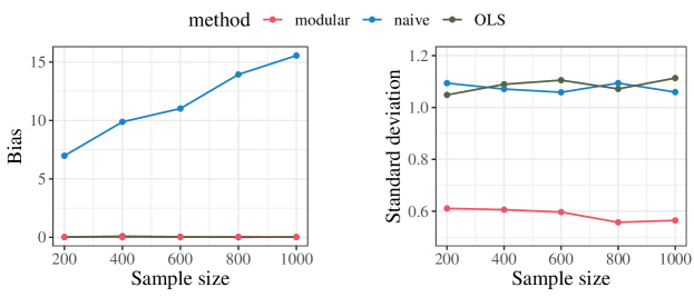
Figure 1: Scaled by $\sqrt{n}$, the bias (on the left) and the standard deviation (on the right) are shown for plain OLS, the naive approach, and our to-be-introduced modular approach, across various sample sizes $n$.

Even in this simple example where random forests should excel, the naive approach exhibits a significantly larger bias compared to plain OLS. This bias is larger than $n^{-1/2}$, and is due to the slow convergence of random forests. In addition, contrary to our prediction, the standard deviation of the naive approach is close to, instead of smaller than, the OLS, which is also due to the variability in training the random forests.

A better approach.

The performance of our new approach is depicted in red in Figure 1: It has negligible bias and reduces the standard deviation by more than $40\%$ compared with OLS at all sample sizes. Our new approach uses the same intuitions as mentioned earlier but additionally addresses bias using well-known semi-parametric techniques based on the mixed-bias property (Rotnitzky et al.,, 2021; Robins et al.,, 2008). We further rewrite (4) as

$$\mathbb{E}[XY]=\mathbb{E}[X\mathbb{E}[Y{\,|\,}Z]]+\mathbb{E}[\mathbb{E}[X|Z]Y]-\mathbb{E}[\mathbb{E}[X{\,|\,}Z]\mathbb{E}[Y{\,|\,}Z]].$$ (6)

Again, an estimator can be obtained via three sub-tasks: (i) estimating $\mathbb{E}[Y|Z=z]$ via $\hat{\mu}_{y}(z)$, (ii) estimating $\mathbb{E}[X|Z=z]$ via $\hat{\mu}_{x}(z)$, and (iii) combining these two estimates via

$$\hat{C}=\frac{1}{n}\sum_{i=1}^{n}\big{\{}\hat{\mu}_{y}(Z_{i})X_{i}+Y_{i}\hat{\mu}_{x}(Z_{i})-\hat{\mu}_{y}(Z_{i})\hat{\mu}_{x}(Z_{i})\big{\}}.$$ (7)

We will show that a slight variation of this approach has very favorable properties. Most importantly, even if $\hat{\mu}_{y}$ and $\hat{\mu}_{x}$ converge to the ground truth at slow speed, the bias of $\hat{C}$ in (7) can still be negligible, and it has a lower variance than $\frac{1}{n}\sum_{i=1}^{n}X_{i}Y_{i}$:

$$n\cdot\operatorname{{\rm Var}}(\hat{C})\approx\operatorname{{\rm Var}}(XY)-\operatorname{{\rm Var}}\big{(}(X-\mu_{x}(Z))\cdot(Y-\mu_{y}(Z))\big{)}\leq\operatorname{{\rm Var}}(XY).$$

Indeed, it leads to the most efficient estimator if $X\perp\!\!\!\perp Y{\,|\,}Z$ (see Section 2.2 for details). This approach also opens a door for data fusion: (7) only involve pairwise observations of $(X,Z)$ or $(Z,Y)$. Thus, it can flexibly use additional data to improve estimation accuracy, and works even when no joint observations of $(X,Z,Y)$ are available.

1.2 A modular regression framework

We propose a modular regression framework that concretize the above ideas by carefully dealing with the nuances in obtaining estimators $\hat{\mu}_{x}$, $\hat{\mu}_{y}$ to eliminate bias, navigating bias-variance tradeoffs under potential violation of the conditional independence assumption, and developing principled algorithms for general estimators and data fusion scenarios.

As the name suggests, we decompose the estimation of $\mathbb{E}[XY]$ into smaller modules – each being a sub-task that involves a subset of variables such as $(Y,X)$, $(Y,Z)$ or $(Z,X)$ – and then re-assemble the modules to construct $\hat{C}$. This idea is visualized in Figure 2.

(a) Conditional independencies can be leveraged to decompose statistical tasks into subtasks.

(b) Modularity allows combining multiple datasets.

Figure 2: Decomposing the estimation of $C=\mathbb{E}[YX]$ tackles two settings that may seem different at first sight. In (a), one can leverage conditional independencies to reduce statistical uncertainty. In (b), one can use additional data to increase effective sample size.

As shown in panel (a), our method adapts to specific structures, such as conditional independence between variables, so as to ensure a properly chosen decomposition. Such structure can also be learned from data. The decomposition also allows data fusion; see panel (b). As long as a data set covers the variables in a sub-task, it can be incorporated to improve efficiency. We summarize our main results below.

• Modular linear regression. We develop a generic approach for improving the estimation and prediction in (generalized) linear models. This is achieved by rewriting the estimation equation to utilize auxiliary variables. Leveraging semi-parametric theory, we show the optimality of our approach under a conditional independence condition.

• High-dimensional modular regression. By adding $\ell_{1}$-regularization, our tools extend to the high-dimensional setting. We develop a proxy empirical risk that has negligible bias and lower variance compared with the Lasso. We show that it improves the upper bounds for prediction accuracy.

• Robustness under conditional dependence. Since the conditional independence condition may be violated in practice, we develop an extension of our method that adapts to the dependency structures among variables, and we allow such structures to be learned from data. The proposed procedure interpolates between linear models (non-modular) and the fully-modular approach (which is efficient under conditional independence). The proposed procedure, bridging linear (non-modular) and fully-modular models, enhances robustness while still allowing for efficiency gains.

• Data fusion. We further extends method to combine multiple data sets. This formulation allows using additional data on sub-tasks to improve overall statistical efficiency.

The rest of the paper is organized as follows. Section 2 develops modular (generalized) linear regression in the fixed-$p$ setting. Section 3 studies modular regression for penalized linear regression in high dimensions, and develops a robust variant that can adapt to different dependence structures. Applications to data fusion and partial observations are discussed in Section 4. Finally, we evaluate our methods on simulated datasets in Section 5 and apply them to real datasets in Section 6.

1.3 Related work

Modular regression combines evidence from sub-tasks, leveraging a “modular structure” provided by the conditional independence. One related strand is to use surrogates when the outcome of interest is expensive to measure (Fleming et al.,, 1994; Post et al.,, 2010). In particular, in causal inference, a series of work (Prentice,, 1989; Lauritzen et al.,, 2004; Chen et al.,, 2007; VanderWeele,, 2013; Athey et al.,, 2016, 2019; Kallus and Mao,, 2020) have advocated using intermediate (short-term) outcome(s) as “surrogates” for long-term outcomes, and assumes various surrogate conditions such as conditional independence of the long-term outcome and the treatment given the surrogates. Similar to our approach, the surrogate condition allows to decompose treatment effect estimation into sub-tasks of estimating the effect of the treatment on the intermediate outcome and estimating the effect of the intermediate outcome on the long-term outcome. We work under a generic conditional independence condition and mainly focus on regression and prediction tasks. In addition, we propose a method that is robust to violations of conditional independence.

Our framework is related to missing data and in particular data fusion, which combines data sets that cover different subsets of variables. The preceding paragraph is also related; more generally, there has been a surge of interest in combining different data sets, such as combining experimental and observational data for treatment effect estimation (Rosenman et al.,, 2022, 2020; Colnet et al.,, 2020), generalizing inference to different populations (Dahabreh et al.,, 2019; Hartman et al.,, 2015; Jin and Rothenhäusler,, 2021), etc. Many of these works require identifiability assumptions for the target estimand, which are similar to the conditional independence condition. Compared to these works, we study general tasks and enjoy robustness to failure of conditional independence.

In missing data scenarios, some other works study regression problem in settings that differ from ours. Those for high-dimensional data include Loh and Wainwright, (2011) on penalized regression, Lounici, (2014); Cai and Zhang, (2016) on the estimation of covariance matrices, and Elsener and van de Geer, (2019); Zhu et al., (2019) on sparse principal component analysis, which consider estimation when some covariates are missing at random. In contrast, we focus more on the data fusion aspect; we draw ideas from semiparametric statistics, and account for the dependence structure. A recent work of Cannings and Fan, (2022) on U-statistics with low-dimensional data is related, which devises an estimator with smaller prediction MSE by incorporating a partially missing data set. Instead, our approach leverages conditional independence structures among variables instead of correlation between estimators; we focus on regression and consider the high dimensional regime.

Our estimator is inspired by recent progress in efficient regression adjustment (Henckel et al.,, 2019; Rotnitzky and Smucler,, 2019) in low-dimensional graphical models. Our framework is more general as it applies to (generalized) linear models, works for high dimensional settings, does not require the graphical structure, and imposes minimal model assumptions; it is also more restricted in that we do not consider choosing the optimal covariate sets.

The modular estimator is optimal for linear regression under conditional independence, in the sense of semiparametric efficiency (Bickel et al.,, 1993; Tsiatis,, 2006). Thus, this work is also connected to the literature of missing data. Furthermore, the double robustness of our estimator is similar to the AIPW estimator (Robins et al.,, 1994) and leverages the “mixed-bias” property (Rotnitzky et al.,, 2021; Robins et al.,, 2008).

The conditional independence structure has been used in a series of early works (Sargan,, 1958; Hansen,, 1982) to improve estimation efficiency; also related is Causeur and Dhorne, (2003) on linear regression under conditional independence, which is closely related to our first modular regression algorithm in low dimensions. However, these works assume strong parametric models such as a joint Gaussian distribution and independent Gaussian noise, while our method does not require stringent model assumptions.

Broadly speaking, our variance reduction idea may also apply to other statistical problems where the ‘modular’ structure and conditional independence are present. For instance, sufficient dimensional reduction (SDR) (Li,, 2018) imposes $Y\perp\!\!\!\perp X{\,|\,}X^{\top}\Gamma$ for some unknown matrix $\Gamma$, whose estimation often relies on inverse regression algorithms (Li,, 1991; Adragni and Cook,, 2009; Ma and Zhu,, 2013) that demonstrate a modular structure. Our idea may be adapted to enable more efficient inverse regression given an approximate solution for $\Gamma$.

Notations.

We use the standard $O_{P}(\cdot)$ and $o_{P}(\cdot)$ notation to denote smaller order in probability. For any two sequences $\{a_{n}\}$ and $\{b_{n}\}$ of positive numbers, we denote $a_{n}=\Omega(b_{n})$ if $\lim_{n\to\infty}a_{n}/b_{n}<\infty$ and $\lim_{n\to\infty}b_{n}/a_{n}<\infty$; we denote $a_{n}=O(b_{n})$ if $a_{n}/b_{n}\leq C$ for some constant $C>0$. We use $\mathbb{P}_{X,Y,Z}$ to denote the joint distribution of $(X,Y,Z)$. For any functions $f,g\colon\mathcal{Z}\to\mathbb{R}^{d}$, we denote their $L_{2}$-distance as $\|f-g\|_{L_{2}(\mathbb{P}_{Z})}^{2}=\mathbb{E}[\|f(Z)-g(Z))\|_{2}^{2}]$, where $\|\cdot\|_{2}$ is the Euclidean norm and the expectation is with respect to the distribution $\mathbb{P}_{Z}$ of $Z$. For any vector $v\in\mathbb{R}^{l}$ and positive definite matrix $\Sigma\in\mathbb{R}^{l\times l}$ we set $\|v\|_{\Sigma}^{2}=v^{\top}\Sigma v$.

2 Modular linear regression in low dimensions

We first introduce modular regression in low-dimensional linear models, where $X\in\mathbb{R}^{p_{x}}$, $Z\in\mathbb{R}^{p_{z}}$, and $p_{x}$, $p_{z}$ do not grow with $n$ asymptotically.

Assumption 2.1.

The joint distribution of $(X,Z,Y)$ satisfies $X\perp\!\!\!\perp Y{\,|\,}Z$.

In this section, we use this working assumption to show how conditional independencies can be leveraged to improve estimation accuracy. It will be relaxed later in Section 3.3, where we develop a method that is robust to violations of Assumption 2.1.

Intuitively, Assumption 2.1 ensures that $Z$ contains all the information in $Y$ that is relevant to $X$. While this assumption seems strong, it is reasonable in many situations and has been widely used in a variety of applications. For example, $Z$ could be an intermediate outcome in the training data that is unavailable for the test samples, while $Y$ is a long-term outcome of interest. Intermediate outcomes are widely used as a proxy in estimating long-term treatment effects (Athey et al.,, 2016, 2019), while we focus on regression problems.

2.1 Modular linear regression

For simplicity of exposition, we start with linear (OLS) regression to show the benefits of a modular structure. Our goal is to predict $Y\in\mathbb{R}$ by $\hat{Y}=X^{\top}\theta$ for some $\theta\in\mathbb{R}^{p_{x}}$, but we do not necessarily assume a well-posed linear model. In the training process, we have observations of i.i.d. triples $\{(X_{i},Y_{i},Z_{i})\}_{i=1}^{n}$ for some auxiliary variables $Z_{i}\in\mathbb{R}^{p_{z}}$, and $X_{i}\in\mathbb{R}^{p_{x}}$ are random vectors (we view all vectors as column vectors throughout). The training and the target distributions are induced by the same distribution $(X,Y,Z)\sim\mathbb{P}$.

Modular regression proceeds in three steps to leverage conditional independence.

1. Decompose into sub-tasks. First, the conditional independence structure in Assumption 2.1 allows us to decompose the estimation of $\mathbb{E}[XY]$ into sub-tasks that only involve observations of $(X,Z)$ or $(Y,Z)$.

2. Solve the sub-tasks. We then learn the conditional mean functions. We use cross-fitting (Chernozhukov et al.,, 2018) to ensure desirable statistical properties: we randomly split $\mathcal{I}=\{1,\dots,n\}$ into two disjoint folds $\mathcal{I}_{1}$, $\mathcal{I}_{2}$. Then for each fold $k=1,2$, we fit models $\hat{\mu}_{x}^{(i)}\colon\mathcal{Z}\to\mathbb{R}^{p_{x}}$ and $\hat{\mu}_{y}^{(k)}\colon\mathcal{Z}\to\mathbb{R}^{p_{y}}$ for $\mu_{x}(z)=\mathbb{E}[X{\,|\,}Z=z]$ and $\mu_{y}(z)=\mathbb{E}[Y{\,|\,}Z=z]$ using data in $\mathcal{I}\backslash\mathcal{I}_{k}$. With slight abuse of notation, we write $\hat{\mu}_{y}(Z_{i})=\hat{\mu}_{y}^{(k)}(Z_{i})$ and $\hat{\mu}_{x}(Z_{i})=\hat{\mu}_{x}^{(k)}(Z_{i})$, $i\in\mathcal{I}_{k}$.

3. Assemble the sub-tasks. Finally, we solve a modular least squares regression

   $$\hat{\theta}_{n}^{\textrm{mod}}=\mathop{\mathrm{argmin}}_{\theta\in\mathbb{R}^{p_{x}}}~{}\bigg{\{}\frac{1}{n}\sum_{i=1}^{n}\theta^{\top}X_{i}X_{i}^{\top}\theta/2-\hat{C}_{\textrm{lm}}^{\top}\theta\bigg{\}},$$ (8)

   where we use a proxy cross-term

   $$\hat{C}_{\textrm{lm}}=\frac{1}{n}\sum_{i=1}^{n}\big{[}X_{i}\hat{\mu}_{y}(Z_{i})+\hat{\mu}_{x}(Z_{i})Y_{i}-\hat{\mu}_{x}(Z_{i})\hat{\mu}_{y}(Z_{i})\big{]}.$$ (9)

The procedure is summarized in Algorithm 1. When $X$ contains an intercept, the corresponding entry of $\hat{C}_{\textrm{lm}}$ can be simply set as $\frac{1}{n}\sum_{i=1}^{n}Y_{i}$.

Algorithm 1 Modular linear regression

0:  Dataset $\mathcal{I}=\{(Y_{i},X_{i},Z_{i}\}_{i=1}^{n}$.

1:  Randomly split $\mathcal{I}$ into equally-sized folds $\mathcal{I}_{k}$, $k=1,2$.

2:  for $k=1,2$ do

3:     Fit models $\hat{\mu}_{x}^{(k)}(\cdot)$ for $\mathbb{E}[X{\,|\,}Z=\cdot]$ using observations $(X_{i},Z_{i})$, $i\notin\mathcal{I}_{k}$;

4:     Fit models $\hat{\mu}_{y}^{(k)}(\cdot)$ for $\mathbb{E}[Y{\,|\,}Z=\cdot]$ using observations $(Y_{i},Z_{i})$, $i\notin\mathcal{I}_{k}$;

5:     Compute $\hat{\mu}_{x}(Z_{i})=\hat{\mu}_{x}^{(k)}(Z_{i})$ and $\hat{\mu}_{y}(Z_{i})=\hat{\mu}_{y}^{(k)}(Z_{i})$ for all $i\in\mathcal{I}_{k}$.

6:  end for

7:  Compute the proxy cross-term $\hat{C}_{\textrm{lm}}$ as in (9).

7:  The modular linear regression $\hat{\theta}_{n}^{\textrm{mod}}$ as in (8).

2.2 Double robustness and semiparametric efficiency

The modular estimator $\hat{\theta}_{n}^{\textrm{mod}}$ is doubly robust with respect to the estimation error of $\hat{\mu}_{x}$ and $\hat{\mu}_{y}$. To be more precise, the estimator converges at $n^{-1/2}$ rate to $\theta^{*}$ and is semiparametrically efficient even when $\hat{\mu}_{x}$ and $\hat{\mu}_{y}$ are consistent with slow nonparametric rates, that is if $\|\hat{\mu}_{x}^{(k)}-\mu_{x}\|_{L_{2}(\mathbb{P}_{Z})}=o_{P}(n^{-1/4})$ and $\|\hat{\mu}_{y}^{(k)}-\mu_{y}\|_{L_{2}(\mathbb{P}_{Z})}=o_{P}(n^{-1/4})$. The proof of the next theorem is in Appendix C.1.

Theorem 2.2 (Double robustness and efficiency).

Suppose $\|\hat{\mu}_{x}^{(k)}-\mu_{x}\|_{L_{2}(\mathbb{P}_{Z})}\cdot\|\hat{\mu}_{y}^{(k)}-\mu_{y}\|_{L_{2}(\mathbb{P}_{Z})}=o_{P}(1/\sqrt{n})$ for $k=1,2$, $\mathbb{E}[XX^{\top}]\succ 0$ is finite, and $X(Y-X^{\top}\theta^{*})$ has finite second moment. Then $\sqrt{n}(\hat{\theta}_{n}^{\textrm{mod}}-\theta^{*})\stackrel{{\scriptstyle d}}{{\to}}N(0,\Sigma^{\textrm{mod}})$ as $n\to\infty$, where $\Sigma^{\textrm{mod}}=\operatorname{\rm Cov}(\phi^{\textrm{mod}}(X_{i},Y_{i},Z_{i}))$ for $\phi^{\textrm{mod}}(x,y,z)=\mathbb{E}[XX^{\top}]^{-1}\big{(}x\mu_{y}(z)+\mu_{x}(z)y-\mu_{x}(z)\mu_{y}(z)-xx^{\top}\theta^{*}\big{)}$. Further, suppose the distribution of $(X,Y,Z)$ has density with respect to a base measure $\mu$. Then $\phi^{\textrm{mod}}$ is the (semiparametrically) efficient influence function for estimating $\theta^{*}$.

A short discussion of the implications of Theorem 2.2 is in order. When $\hat{\mu}_{x}$ and $\hat{\mu}_{y}$ are estimated by nonparametric regression which typically comes with slow rates, Assumption 2.1 (conditional independence) is needed to ensure fast convergence of $\hat{\theta}_{n}^{\textrm{mod}}$. However, when they are estimated by parametric regression (such as OLS) and converge at $\sqrt{n}$-rate to any $\mu_{x}^{*}$ and $\mu_{y}^{*}$ (not necessarily equal $\mu_{x}$ or $\mu_{y}$), our estimator is consistent and asymptotically normal with $\sqrt{n}$-rate as long as $\mathbb{E}[(Y-\mu_{y}^{*}(Z))(X-\mu_{x}^{*}(Z))]=0$, i.e., the residuals of $Y$ and $X$ are uncorrelated. This effect will also be visible in our simulations in Section 5.

Theorem 2.2 shows that modular regression has the lowest asymptotic variance among all regular estimators (Bickel et al.,, 1993). We now compare it with the OLS estimator $\hat{\theta}_{n}^{\textrm{ols}}=\mathop{\mathrm{argmin}}_{\theta\in\mathbb{R}^{d}}~{}\sum_{i=1}^{n}(Y_{i}-X_{i}^{\top}\theta)^{2}$, which only uses the information in $(X_{i},Y_{i})$ pairs. We know $\hat{\theta}_{n}^{\textrm{ols}}-\theta^{*}=\frac{1}{n}\sum_{i=1}^{n}\phi^{\textrm{ols}}(X_{i},Y_{i})+o_{P}(1/\sqrt{n})$ with $\phi^{\textrm{ols}}(x,y)=\mathbb{E}[XX^{\top}]^{-1}(xy-xx^{\top}\theta^{*})$ as $n\to\infty$. Under Assumption 2.1, the asymptotic variance of $\phi^{\textrm{mod}}(X_{i},Y_{i},Z_{i})$ is dominated by that of $\phi^{\textrm{ols}}(X_{i},Y_{i})$. Indeed, one can check that

$$\operatorname{\rm Cov}\big{(}\phi^{\textrm{mod}}(X_{i},Y_{i},Z_{i})\big{)}=\operatorname{\rm Cov}\big{(}\phi^{\textrm{ols}}(X_{i},Y_{i})\big{)}-\Sigma^{-1}\operatorname{\rm Cov}\big{(}(Y-\mu_{y}(Z))(X-\mu_{x}(Z)\big{)}\Sigma^{-1},$$

where $\operatorname{\rm Cov}(A)$ denotes the covariance matrix for a random vector $A$, so that $\operatorname{\rm Cov}\big{(}(Y-\mu_{y}(Z))(X-\mu_{x}(Z)\big{)}\succ 0$. More efficient parameter estimation also translates to more accurate prediction: The prediction mean squared error (MSE) for an independent test sample $(X,Y)$ is $\mathbb{E}[(Y-X^{\top}\hat{\theta})^{2}{\,|\,}\hat{\theta}]=\mathbb{E}[(Y-X^{\top}\theta^{*})^{2}]+\|\hat{\theta}-\theta^{*}\|_{\Sigma}^{2}$, where the second term is smaller when $\hat{\theta}$ is the modular estimator instead of the OLS estimator. In our numerical experiments, we mostly focus on improving prediction in very noisy settings with low sample size because the improvement in $\|\hat{\theta}-\theta^{*}\|_{\Sigma}^{2}$ is more pronounced in those cases.

Remark 2.3 (Alternative estimators).

There are several natural alternatives to our modular estimator. The first is outcome regression, i.e., running OLS of $\hat{\mu}_{y}(Z_{i})$ over $X_{i}$, where $\hat{\mu}_{y}(\cdot)$ is an estimator for $\mu_{y}(\cdot)=\mathbb{E}[Y{\,|\,}Z=\cdot]$. The second is orthogonal regression, i.e., extracting the $X$-coefficients in OLS of $Y_{i}$ over $(X_{i},Z_{i}^{\rm resid})$, where $Z^{\rm resid}:=Z_{i}-\mu_{z}(X_{i})$, and $\hat{\mu}_{z}(\cdot)$ is an estimator for $\mu_{z}(\cdot)=\mathbb{E}[Z{\,|\,}X=\cdot]$. However, both options can be less efficient than our proposals. When $\hat{\mu}_{y}$ and $\hat{\mu}_{z}$ are estimated by flexible nonparametric algorithms, both methods suffer from substantial bias that is comparable to or larger than the OLS variance (this is similar to the issue with our naive approach in Section 1); in contrast, our estimator achieves fast (product) convergence rate, and is the most efficient among all regular and asymptotically linear estimators. An extended discussion is in Appendix B.2.

Practitioners may be interested in quantifying the uncertainty of modular regression estimates. Wald-type confidence intervals can be derived using the asymptotic distribution in Theorem 2.2. The next corollary formalizes this result for the one-dimensional case; the multi-dimensional case follows similar ideas.

Corollary 2.4 (Confidence intervals).

When $p_{x}=1$, set $\hat{\rm CI}:=\hat{\theta}_{n}^{\textrm{mod}}\pm z_{1-\alpha/2}\hat{\sigma}_{n}^{\textrm{mod}}/\sqrt{n}$, where $(\hat{\sigma}_{n}^{\textrm{mod}})^{2}=\frac{1}{n}\sum_{i=1}^{n}(d_{i}-\bar{d})^{2}$ for $\bar{d}=\frac{1}{n}\sum_{i=1}^{n}d_{i}$, and $d_{i}:=\hat{\mathbb{E}}[XX^{\top}]^{-1}\big{(}X_{i}\hat{\mu}_{y}(Z_{i})+\hat{\mu}_{x}(Z_{i})Y_{i}-\hat{\mu}_{x}(Z_{i})\hat{\mu}_{y}(Z_{i})-X_{i}X_{i}^{\top}\hat{\theta}_{n}^{\textrm{mod}}\big{)}$ from Algorithm 1. Here, $z_{1-\alpha/2}$ denotes the $1-\alpha/2$ quantile of a standard Gaussian random variable. Then, under the conditions of Theorem 2.2, $(\hat{\sigma}_{n}^{\textrm{mod}})^{2}\stackrel{{\scriptstyle P}}{{\to}}\operatorname{{\rm Var}}(\phi^{\textrm{mod}}(X,Y,Z))$, and thus $\mathbb{P}(\theta^{*}\in\hat{\rm CI})\to 1-\alpha$ as $n\to\infty$.

One may also learn and adapt to the dependence structure from data (see Section 3.3 for a related discussion). In such cases, confidence intervals have to be adjusted to account for the variation induced by estimation of the structure. In practice, one can deal with this issue by data-splitting (i.e., use one fold of data for model selection and the second for estimation) and cross-fitting (Chernozhukov et al.,, 2018).

Remark 2.5 (Efficiency gain over OLS).

To gain more intuition on the improvement in parameter estimation, we consider a one-dimensional special case where $Z=\alpha X+\epsilon_{z}$, $Y=\beta Z+\epsilon_{y}$ for $\alpha,\beta\in\mathbb{R}$. Here $X\sim N(0,\sigma_{x}^{2})$, and $\epsilon_{z}\sim N(0,\sigma_{z}^{2})$, $\epsilon_{y}\sim N(0,\sigma_{y}^{2})$ are independent random noise. The true parameter for OLS regression is $\theta^{*}=\alpha\beta$. The OLS estimator $\hat{\theta}_{n}^{\textrm{ols}}$ has asymptotic variance $\sigma_{\textrm{ols}}^{2}=\operatorname{{\rm Var}}(X)^{-2}\operatorname{{\rm Var}}(X\epsilon_{y}+X\beta\epsilon_{z})=\operatorname{{\rm Var}}(X)^{-1}(\sigma_{y}^{2}+\beta^{2}\sigma_{z}^{2})$, and our modular estimator $\hat{\theta}_{n}^{\textrm{mod}}$ has asymptotic variance $\sigma_{\textrm{mod}}^{2}=\operatorname{{\rm Var}}(X)^{-2}\operatorname{{\rm Var}}(\mu_{x}(Z)\epsilon_{y}+X\beta\epsilon_{z})=\operatorname{{\rm Var}}(X)^{-1}(\sigma_{y}^{2}\frac{\operatorname{{\rm Var}}(\mu_{x}(Z))}{\operatorname{{\rm Var}}(X)}+\beta^{2}\sigma_{z}^{2})$. That is, the absolute improvement in asymptotic variance is $\sigma_{\textrm{ols}}^{2}-\sigma_{\textrm{mod}}^{2}=\sigma_{y}^{2}\frac{\operatorname{{\rm Var}}(X-\mu_{x}(Z))}{\sigma_{x}^{4}}$; this quantity is large if $\sigma_{y}^{2}$ is large or $Z$ explains a small proportion of the variance in $X$, i.e., $\operatorname{{\rm Var}}(X-\mu_{x}(Z))$ is large compared to $\sigma_{x}^{2}$. The relative improvement in asymptotic variance is $1-\frac{\sigma_{\textrm{mod}}^{2}}{\sigma_{\textrm{ols}}^{2}}=\frac{1}{1+\alpha^{2}\sigma_{x}^{2}/\sigma_{z}^{2}}\frac{1}{1+\beta^{2}\sigma_{z}^{2}/\sigma_{y}^{2}}$; this quantity is large if $\alpha^{2}\frac{\sigma_{x}^{2}}{\sigma_{z}^{2}}$ and $\beta^{2}\frac{\sigma_{z}^{2}}{\sigma_{y}^{2}}$ are small, which corresponds to (i) weak signal $\alpha,\beta$, or (ii) large noise $\sigma_{z}^{2}$ compared to $\sigma_{x}^{2}$, and $\sigma_{y}^{2}$ compared to $\sigma_{z}^{2}$. In the most extreme case where $\alpha=\beta=0$, the best prediction is $0$, and we achieve the asymptotic variance $\sigma_{\textrm{mod}}^{2}=0$.

Our discussion so far is mainly asymptotic, so that the bias incurred by the estimation error of $\hat{\mu}_{x}$ and $\hat{\mu}_{y}$ is negligible compared to the $O(1/\sqrt{n})$ statistical error. Next, we use a simple example to provide insights on the finite sample behavior of $\hat{\theta}_{n}^{\textrm{mod}}$ and $\hat{\theta}_{n}^{\textrm{ols}}$.

Remark 2.6 (Finite-sample efficiency).

We assume $(X,Y,Z)\in\mathbb{R}^{3}$ are jointly Gaussian, and $\hat{\mu}_{x}$ and $\hat{\mu}_{y}$ are estimated by OLS. Given OLS’s $O_{P}(1/\sqrt{n})$ consistency, we forego cross-fitting to prevent cumbersome calculations. As a result, $\hat{\mu}_{x}(z)=\hat{\mathbb{E}}_{n}[Z^{2}]^{-1}\hat{\mathbb{E}}_{n}[XZ]z$, and $\hat{\mu}_{y}(z)=\hat{\mathbb{E}}_{n}[Z^{2}]^{-1}\hat{\mathbb{E}}_{n}[YZ]z$, where $\hat{\mathbb{E}}_{n}[\cdot]$ denotes empirical mean over all the data. One can then check that $\hat{\theta}_{n}^{\textrm{mod}}=\hat{\mathbb{E}}_{n}[X^{2}]^{-1}\hat{\mathbb{E}}_{n}[Z^{2}]^{-1}\hat{\mathbb{E}}_{n}[YZ]\hat{\mathbb{E}}_{n}[XZ]$ and $\hat{\theta}_{n}^{\textrm{ols}}=\hat{\mathbb{E}}_{n}[X^{2}]^{-1}\hat{\mathbb{E}}_{n}[YX]$. By joint Gaussianity, there exists some $\alpha,\beta\in\mathbb{R}$ such that $X=\alpha Z+\epsilon_{x}$ and $Y=\beta Z+\epsilon_{y}$, where $\epsilon_{x}\sim N(0,\sigma_{x}^{2})$ and $\epsilon_{y}\sim N(0,\sigma_{y}^{2})$ conditional on $Z$. Both $\hat{\theta}_{n}^{\textrm{mod}}$ and $\hat{\theta}_{n}^{\textrm{ols}}$ are unbiased for $\theta^{*}$, while $\operatorname{{\rm Var}}(\hat{\theta}_{n}^{\textrm{ols}})-\operatorname{{\rm Var}}(\hat{\theta}_{n}^{\textrm{mod}})=\sigma_{y}^{2}\mathbb{E}\big{[}\frac{\hat{\mathbb{E}}_{n}[Z^{2}]\cdot\hat{\mathbb{E}}_{n}[\epsilon_{x}^{2}]-\hat{\mathbb{E}}_{n}[Z\epsilon_{x}]^{2}}{n(\hat{\mathbb{E}}_{n}[X^{2}])^{2}\cdot\hat{\mathbb{E}}_{n}[Z^{2}]}\big{]}\geq 0$. That is, in finite sample, $\hat{\theta}_{n}^{\textrm{mod}}$ is always more efficient than $\hat{\theta}_{n}^{\textrm{ols}}$. See detailed calculation and discussion in Appendix B.1.

2.3 Modular regression in generalized linear models

The ideas outlined in the previous section also apply to generalized linear models (GLMs) as long as the estimation equation has a modular structure.

Following the general setup in Section 1, we suppose the true parameter $\theta^{*}\in\Theta\subseteq\mathbb{R}^{p_{x}}$ is the unique minimizer of $\mathbb{E}\big{[}\ell(X_{i},Y_{i},\theta^{*})\big{]}$, where $\ell(x,y,\theta)=YX^{\top}\theta+h(x,\theta)$ for some function $h\colon\mathcal{X}\times\Theta\to\mathbb{R}^{p}$ that is convex in $\theta$. A default estimator $\hat{\theta}_{n}^{\textrm{ml}}$ is the unique minimizer of the empirical loss (1). Maximum likelihood estimation for GLMs with $\log$ links satisfies this condition in general, such as logistic regression with $\ell(x,y,\theta)=-x^{\top}\theta y+\log(1+\exp(x^{\top}\theta))$ for $y\in\{0,1\}$, and Poisson regression with $\ell(x,y,\theta)=-x^{\top}\theta y+\exp(x^{\top}\theta)$ for $y\in\mathbb{N}$. More generally, for exponential regression with $\ell(x,y,\theta)=2\log y\cdot\theta^{\top}x-(\theta^{\top}x)^{2}$ for $y\in\mathbb{R}^{+}$, one can use the transformed outcome $\tilde{Y}:=2\log(Y)$ to make it a special case of equation (1).

To obtain a more accurate estimator for $C=\mathbb{E}[XY]$, the first two steps are exactly the same as in Section 2.1. In the third step, we use $\hat{C}_{\textrm{lm}}$ defined in (9), and compute

$$\hat{\theta}_{n}^{\textrm{mod}}=\mathop{\mathrm{argmin}}_{\theta\in\Theta}~{}\bigg{\{}\frac{1}{n}\sum_{i=1}^{n}h(X_{i},\theta)+\hat{C}_{\textrm{lm}}^{\top}\theta\bigg{\}}.$$ (10)

This estimator is again doubly-robust to the error of $\hat{\mu}_{x}$ and $\hat{\mu}_{y}$, and has smaller asymptotic variance than $\hat{\theta}_{n}^{\textrm{ml}}$ under mild conditions. Its theoretical justification follows similar ideas as before with slightly more involved technical conditions; we defer all the results to Appendix A.

3 Modular linear regression in high dimensions

Many prediction problems involve a huge number of predictive variables, entering the high-dimensional regime where $p_{x}$ grows with, and can even be large than, the sample size $n$. A popular approach to dealing with high-dimensional data is penalized regression such as the Lasso (Tibshirani,, 1996). By assuming a sparse linear regression function, high-dimensional regression has been shown to be consistent under various well-conditioning assumptions (Candes and Tao,, 2005, 2007; Van de Geer,, 2007; Zhang and Huang,, 2008).

Our modular regression idea extends naturally to the high-dimensional setting. In this section, we show that by including an $\ell_{1}$ penalty, modular regression improves upon the Lasso by seeking for a more efficient estimation equation. Throughout this section, we assume a sparse linear model to ensure the task is tractable.

Assumption 3.1.

There exists some $\theta^{*}\in\mathbb{R}^{p_{x}}$ with $\|\theta^{*}\|_{0}=s$, such that $\mathbb{E}[Y{\,|\,}X]=X^{\top}\theta^{*}$.

3.1 Regularized modular regression

We start with cross-fitting, and let $\hat{\mu}_{x}^{(k)}$, $\hat{\mu}_{y}^{(k)}$ be estimators for $\mu_{x}(\cdot)=\mathbb{E}[X{\,|\,}Z=\cdot]$ and $\mu_{y}(\cdot)=\mathbb{E}[Y{\,|\,}Z=\cdot]$ obtained from $\mathcal{I}\backslash\mathcal{I}_{k}$, and define the cross-terms as in (9). The only distinction from Section 2.1 is that we encourage sparsity by $\ell_{1}$-regularization. We left

$$\hat{\theta}_{n}^{\textrm{mod}}=\mathop{\mathrm{argmin}}_{\theta\in\mathbb{R}^{p_{x}}}~{}\bigg{\{}\frac{1}{n}\sum_{i=1}^{n}\theta^{\top}X_{i}X_{i}^{\top}\theta/2-\hat{C}_{\textrm{lm}}^{\top}\theta+\lambda\|\theta\|_{1}\bigg{\}}$$ (11)

for some regularization parameter $\lambda>0$, where $\|\theta\|_{1}=\sum_{j=1}^{p_{x}}|\theta_{j}|$. As (11) is convex in $\theta$, the optimization can be efficiently solved similarly to the Lasso (e.g. coordinate descent). In practice, $\lambda$ can be determined by cross validation.

3.2 Theoretical guarantee

With proper choice of $\lambda$, modular regression leads to a sharper upper bound on the estimation error. We assume a $\mu$-RSC property for the design matrix $X\in\mathbb{R}^{n\times p_{x}}$ which is standard in the literature for the consistency of Lasso-type methods (Bickel et al.,, 2009; Negahban et al.,, 2012). Our theoretical analysis may be generalized to other conditions, which is beyond the scope of this work.

Assumption 3.2.

$X\in\mathbb{R}^{n\times p_{x}}$ obeys $\zeta$-Restricted Strong Convexity ($\zeta$-RSC), i.e., $\|X\Delta\|_{2}^{2}/n\geq\zeta\|\Delta\|_{2}^{2}$ for any $\Delta\in\mathbb{C}_{3}$, where $\mathbb{C}_{3}:=\big{\{}x\in\mathbb{R}^{p}\colon\|x_{S^{c}}\|_{1}\leq 3\|x_{S}\|_{1}\big{\}}$, and $S=\{j\colon\theta_{j}^{*}\neq 0\}$.

We assume entries of $X$ and the response $Y$ are bounded by constants. This condition is mild since the Lasso is often implemented after normalization.

Assumption 3.3.

$|X_{j}|\leq 1$ and $\|\hat{\mu}_{x,j}^{(k)}(\cdot)\|_{\infty}\leq 1$ almost surely for $k=1,2$ and all $1\leq j\leq p$. Also, $|Y_{i}|\leq c_{0}$ and $\|\hat{\mu}_{y}^{(k)}(\cdot)\|_{\infty}\leq c_{0}$ almost surely for $k=1,2$ for some constant $c_{0}>0$.

Finally, we assume $\hat{\mu}_{y}^{(k)}$ and $\hat{\mu}_{x}^{(k)}$ are consistent with $o(n^{-1/4})$ convergence rates.

Assumption 3.4.

Suppose $\|\hat{\mu}_{y}^{(k)}(\cdot)-\mu_{y}(\cdot)\|_{L_{2}(\mathbb{P}_{Z})}=o_{P}(n^{-1/4})$ for $k=1,2$. Also, there exists a sequence of constants $c_{n}\to 0$ such that for sufficiently large $n$,

$$\max_{1\leq j\leq p_{x},k=1,2}\mathbb{P}\bigg{(}\big{\|}\hat{\mu}_{x,j}^{(k)}(\cdot)-\mu_{x,j}(\cdot)\big{\|}_{L_{2}(\mathbb{P}_{Z})}\geq\frac{c_{n}\log(1/\delta)}{n^{1/4}}\bigg{)}\leq\delta.$$ (12)

Here $\hat{\mu}_{x,j}^{(k)}(\cdot)$ is the $j$-th entry of $\hat{\mu}_{x}^{(k)}$, an estimator for $\mu_{x,j}(\cdot):=\mathbb{E}[X_{j}{\,|\,}Z=\cdot]$.

Assumption 3.4 slightly differs from the commonly adopted consistency conditions, which is often of the form $\|\hat{\mu}_{x,j}^{(k)}-\mu_{x,j}\|_{L_{2}(\mathbb{P}_{Z})}=o_{P}(n^{-1/4})$, on the estimation of nuisance components. This is because we need an exponential tail bound to control all $2\times p_{x}$ estimated functions $\{\hat{\mu}_{x,j}^{(k)}\}_{j=1,k=1}^{p_{x},2}$ simultaneously. Running many regressions may incur considerable computational cost in high dimensions; we provide a computational shortcut in Section 3.4.

Many estimators in the literature obey Assumption 3.4. When $Z$ is high-dimensional (i.e., $p_{z}$ may grow with $n$ or be larger than $n$), if $\mathbb{E}[X_{j}{\,|\,}Z]$ is an $s^{\prime}$-sparse linear function of $Z$, then (12) holds for the Lasso estimator with $c_{n}\asymp\sqrt{s^{\prime}\log(p_{z})}/n^{1/4}$ when the regularization parameter is properly chosen. When $Z$ is low-dimensional (i.e., $p_{z}$ does not grow with $n$), under the standard assumption that $\mathbb{E}[X_{j}{\,|\,}Z]$ is sufficiently smooth, the well-established convergence results of sieve estimation can be turned into such bounds by exponential tail bounds for the concentration of empirical loss functions (Chen and Shen,, 1998; Chen,, 2007).

We show an improved bound for the estimation error of $\hat{\theta}_{n}^{\textrm{mod}}$ compared to the Lasso estimator using $(X_{i},Y_{i})$. The proof of Theorem 3.5 is in Appendix C.2.

Theorem 3.5 (Finite-sample bound).

Suppose Assumptions 2.1, 3.2, 3.3 and 3.4 hold. Then there exists a sequence of constants $\{\bar{c}_{n}\}$ with $\bar{c}_{n}\to 0$ as $n\to\infty$, such that for any fixed $\delta\in(0,1)$ and any regularization parameter $\lambda$ obeying

$$\lambda\geq\frac{2}{n}\big{\|}\mu_{y}^{\top}X+Y^{\top}\mu_{x}-\mu_{y}^{\top}\mu_{x}-(X\theta^{*})^{\top}X\big{\|}_{\infty}+\frac{\bar{c}_{n}(\log(3p_{x}/\delta))^{2}}{\sqrt{n}},$$ (13)

it holds with probability at least $1-\delta$ that

$$\|\hat{\theta}_{n}^{\textnormal{{mod}}}-\theta^{*}\|_{2}\leq\frac{3\lambda\sqrt{s}}{2\zeta}.$$

Here we denote $\|z\|_{\infty}=\sup_{j}|z_{j}|$, $Y,\mu_{y}\in\mathbb{R}^{n}$ are vectors whose $i$-th entries are $Y_{i}$ and $\mu_{y}(Z_{i})$, and $X,\mu_{x}\in\mathbb{R}^{n\times p_{x}}$ are matrices whose $(i,j)$-th entries are $X_{ij}$ and $\mu_{x,j}(Z_{i})$.

The second term in (13) arises from the estimation error in $\hat{\mu}_{y}$ and $\hat{\mu}_{x}$. It enjoys a double robustness property that is similar to the low-dimensional case: under the slow convergence rate in Assumption 3.4, this error is negligible compared to the first term in (13) that is typically $\Omega(\sqrt{(\log p_{x})/n})$ (Vershynin,, 2018). The estimation error of $\hat{\theta}_{n}^{\textrm{mod}}$ is then characterized by the first term in (13).

When $n$ is sufficiently large such that the second term in (13) is negligible, the deviation of the first term can be decided by the variance of each entry. We define the random vector $\epsilon^{\textrm{mod}}:=X^{\top}\theta^{*}X-\mu_{y}(Z)X-Y\mu_{x}(Z)+\mu_{y}(Z)\mu_{x}(Z)\in\mathbb{R}^{p_{x}}$. Then, in Theorem 3.5, choosing $\lambda\asymp L\sqrt{\max_{j}\operatorname{{\rm Var}}(\epsilon_{j}^{\textrm{mod}})\cdot\log(p_{x})/n}$ yields the estimation error

$$\|\hat{\theta}_{n}^{\textnormal{{mod}}}-\theta^{*}\|_{2}\leq\frac{L\cdot\sqrt{s\log(p_{x})}}{\sqrt{n}\mu}\sqrt{\max_{j}\operatorname{{\rm Var}}(\epsilon_{j}^{\textrm{mod}})},$$ (14)

where $L>0$ is a universal constant. On the other hand, we let $\hat{\theta}_{n}^{\textrm{Lasso}}$ be the Lasso estimator (2). Under similar conditions like Assumption 3.2, existing results in the literature (Negahban et al.,, 2012) show that $\|\hat{\theta}_{n}^{\textrm{Lasso}}-\theta^{*}\|_{2}\leq\frac{3\lambda\sqrt{s}}{2\mu}$ for any regularization parameter obeying $\lambda\geq\big{\|}\frac{2}{n}\sum_{i=1}^{n}(Y_{i}-X_{i}^{\top}\theta^{*})X_{i}\big{\|}_{\infty}.$ We define $\epsilon^{\textrm{Lasso}}=X(Y-X^{\top}\theta^{*})$. Similarly, choosing $\lambda\asymp L\sqrt{\max_{j}\operatorname{{\rm Var}}(\epsilon_{j}^{\textrm{Lasso}})\cdot\log(p_{x})/n}$ yields

$$\|\hat{\theta}_{n}^{\textnormal{{Lasso}}}-\theta^{*}\|_{2}\leq\frac{L\cdot\sqrt{s\log(p_{x})}}{\sqrt{n}\mu}\sqrt{\max_{j}\operatorname{{\rm Var}}(\epsilon_{j}^{\textrm{Lasso}})},$$ (15)

where $L>0$ is the same universal scaling as above. The bounds in (14) and (15) distinguish our modular estimator from the Lasso, as one can check that $\operatorname{{\rm Var}}(\epsilon_{j}^{\textrm{mod}})\leq\operatorname{{\rm Var}}(\epsilon_{j}^{\textrm{Lasso}})$ for all $j$. That is, modular regression reduces the uncertainty by a constant order.

Though this is only an upper bound analysis, our numerical experiments later on confirm the improvement in estimation accuracy. In particular, we will see that the regularization parameter $\lambda$ chosen by cross-validation is smaller in modular regression. Intuitively, the reduction in $\text{Var}(\epsilon_{j}^{\text{mod}})$ allows cross-validation to choose a smaller $\lambda$ than for the Lasso.

Interested readers may wonder whether the modular idea can be leveraged to construct more efficient confidence intervals following the ‘debiasing’ Lasso ideas (Zhang and Zhang,, 2014; Javanmard and Montanari,, 2014; Van de Geer et al.,, 2014). While this may be feasible, this problem warrants a careful and rigorous investigation that is beyond the scope of this work. In addition, structure learning (which we introduce in the next part) may lead to irregular estimators that deserve extra care. In the current paper, we mainly focus on the estimation and prediction aspects, and leave this point for future work.

3.3 Robustness to the conditional independence condition

In practice, Assumption 2.1 may be violated, and the true dependence structure among the variables may be completely unknown. In this part, we generalize our modular regression framework to estimate and adapt to the conditional independence structure.

To be precise, Assumption 2.1 posits that $X_{j}\perp\!\!\!\perp Y{\,|\,}Z$ for every $j$. That is, $Z$ captures all the predictive power of every $X_{j}$ for $Y$. This condition can be violated in many ways. For instance, $Z$ may capture all the information for a subset of variables in $X$, while others in $X$ still have direct effects for $Y$. In this subsection, we assume that $X\perp\!\!\!\perp Y{\,|\,}(Z,X_{\mathcal{J}})$ for some subset $\mathcal{J}\subseteq\{1,\dots,p_{x}\}$, and $X_{\mathcal{J}}$ is the vector containing $X_{j}$ for all $j\in\mathcal{J}$. The choice of $\mathcal{J}$ can be from prior knowledge, or by estimating (consistently) the dependence structure among all the variables when joint observations of $(X,Z,Y)$ are available. Learning the conditional independence structure is beyond our focus; popular methods in the literature include constraint-based (Spirtes et al.,, 2000; Margaritis and Thrun,, 1999; Tsamardinos et al.,, 2006), score-based (Lam and Bacchus,, 1994; Jordan,, 1999; Friedman et al.,, 1999), and regression-based (Lee et al.,, 2006; Meinshausen and Bühlmann,, 2006; Roth,, 2004; Banerjee et al.,, 2006) ones assuming a high-dimensional graphical model, to name a few.

Remark 3.6 (Recommendation in practice).

For high-dimensional linear regression, a heuristic idea is to use the Lasso for structure learning. For example, one can regress $Y$ on $(X,Z)$ via the Lasso, and use all features in $X$ with nonzero estimated coefficient as $X_{\mathcal{J}}$. In our numerical experiments in Section 5, We find that this heuristic approach works well in improving estimation accuracy.

In the following, we outline how to use the output from structure learning such as in Remark 3.6 in conjunction with modular regression. The condition $X\perp\!\!\!\perp Y{\,|\,}(Z,X_{\mathcal{J}})$ can be seen as a special case of Assumption 2.1 for a different choice of the conditioning set “$Z$”:

$$X\perp\!\!\!\perp Y{\,|\,}Z^{\textrm{full}},\quad\textrm{where}\quad Z^{\textrm{full}}=(Z,X_{\mathcal{J}}).$$ (16)

This again allows us to break the problem into sub-tasks. In learning $\mu_{y}$, after data splitting, for each $k=1,2$, we aim $\hat{\mu}_{y}^{(k)}$ for $\mathbb{E}[Y{\,|\,}Z^{\textrm{full}}]$ using data in $\mathcal{I}\backslash\mathcal{I}_{k}$, instead of $\mathbb{E}[Y{\,|\,}Z]$. We only learn $(\mu_{x})_{j}$ for $j\notin\mathcal{J}$: we let $\hat{\mu}_{x,j}^{(k)}(x)$ be an estimate for $\mathbb{E}[X_{j}{\,|\,}Z^{\textrm{full}}]$ using the data in $\mathcal{I}\backslash\mathcal{I}_{k}$ for $k=1,2$. Then for each $i\in\mathcal{I}_{k}$, we compute the cross-term $C_{i}$ via

$$(C_{i})_{j}=\begin{cases}(X_{i})_{j}\hat{\mu}_{y}^{(k)}(Z_{i}^{\textrm{full}})+\hat{\mu}_{x,j}^{(k)}(Z_{i}^{\textrm{full}})Y_{i}-\hat{\mu}_{x,j}^{(k)}(Z_{i}^{\textrm{full}})\hat{\mu}_{y}^{(k)}(Z_{i}^{\textrm{full}}),\quad\text{if }j\notin\mathcal{J},\\[6.45831pt] (X_{i})_{j}Y_{i},\quad\text{if }j\in\mathcal{J}.\end{cases}$$ (17)

Finally, we solve the same modular least squares (8) or penalized least squares (11) with $\hat{C}_{\textrm{lm}}:=\frac{1}{n}\sum_{i=1}^{n}C_{i}$ for the above $C_{i}$. When Assumption 2.1 is violated, the original $\hat{C}_{\textrm{lm}}$ defined in (9) might be biased even if the estimators for conditional expectations are correct. In contrast, the new cross-terms we derive in (17) are unbiased for $(X_{i})_{j}Y_{i}$ with potentially smaller variance under the generalized condition (16).

Let $\hat{J}$ be the output of the structure learning step, and set $Z^{\hat{\textrm{full}}}=(X_{\hat{J}},Z)$. We note that $Y\perp\!\!\!\perp X{\,|\,}Z^{\hat{\textrm{full}}}$ holds with probability tending to 1 if $\hat{J}$ converges in probability to some superset $\tilde{J}\supseteq\mathcal{J}$, our asymptotic expansion in Theorems 2.2 and 3.5 holds on an event with probability tending to 1, and theoretical guarantees for this approach can be directly implied in view of (16) and the fact that the definition of $C_{i}$ in (17) is equivalent to taking $\hat{\mu}_{x,j}^{(k)}(Z_{i}^{\textrm{full}}):=(X_{i})_{j}$, which we omit here. The convergence of $\hat{J}$ can be obtained under, e.g., irrepresentability-type conditions (Zhao and Yu,, 2006), and is typically compatible with Assumption 3.4; see Appendix B.3 for a more detailed discussion.

This variant can be viewed as a data-driven interpolation between the fully modular regression we introduce in the preceding part and the standard OLS or Lasso. If the conditional independence condition holds for $X_{j}$, then utilizing the information in $Z^{\textrm{full}}$ reduces the estimation error in $[\hat{\theta}_{n}^{\textrm{mod}}]_{j}$; otherwise, it reduces to $[\hat{\theta}_{n}^{\textrm{mod}}]_{j}=[\hat{\theta}_{n}^{\textrm{ols}}]_{j}$ in the low-dimensional case, and yields a similar bound as $\hat{\theta}_{n}^{\textrm{Lasso}}$ for the high-dimensional regression.

In general, there is a trade-off between the robustness (related to accuracy of $\hat{J}$) and efficiency gain of $\hat{\theta}_{n}^{\textrm{mod}}$. When $\hat{J}=J$, $\hat{\theta}_{n}^{\textrm{mod}}$ achieves the most efficiency gain. When $\hat{J}=\{1,\dots,p\}$, then $\hat{\theta}_{n}^{\textrm{mod}}$ reduces to $\hat{\theta}_{n}^{\textrm{mod}}$ without any improvement.

Our simulation studies in Section 5 show that this approach robustly improves the estimation and prediction accuracy in cases where Assumption 2.1 is violated but the conditional independence structure (16) may be learned from the data.

3.4 Practical implementation via linear transformation

We now discuss a computational shortcut for high-dimensional modular regression. By using linear transformations for estimating the conditional mean functions, it reduces the computational costs and is readily compatible with standard implementation of the Lasso (e.g., glmnet R-package (Friedman et al.,, 2010)).

First, let us discuss why the estimator as defined in equation (11) is computationally demanding. Note that the modular estimator (11) minimizes

$$\frac{1}{n}\big{\{}\theta^{\top}X^{\top}X\theta/2-\hat{\mu}_{y}^{\top}X\theta-Y^{\top}\hat{\mu}_{x}\theta+\hat{\mu}_{y}^{\top}\hat{\mu}_{x}\theta\big{\}}+\lambda\|\theta\|_{1}$$ (18)

where $\hat{\mu}_{x}\in\mathbb{R}^{n\times p_{x}}$ is a matrix whose $(i,j)$-th entry stores an estimator for $\mu_{x,j}(Z_{i})$, and $\hat{\mu}_{y}\in\mathbb{R}^{n}$ is a vector whose $i$-th entry is an estimator for $\mu_{y}(Z_{i})$. In the cross-fitting approach we outline in Section 3.1, the estimators are specified as $[\hat{\mu}_{x}]_{i,j}=\hat{\mu}_{x,j}^{(k)}(Z_{i})$ and $[\hat{\mu}_{y}]_{i}=\hat{\mu}_{y}^{(k)}(Z_{i})$ for $i\in\mathcal{I}_{k}$. That is, we need to run $\Omega(p_{x})$ times of regression to obtain $\hat{\mu}_{x}^{(k)}$ and $\hat{\mu}_{y}^{(k)}$.

Here, we take a different approach to estimating $\mu_{x}$ and $\mu_{y}$:

$$\hat{\mu}_{x}=\bm{\Pi}_{x}X,\quad\hat{\mu}_{y}=\bm{\Pi}_{y}Y,$$

where $\bm{\Pi}_{x},\bm{\Pi}_{y}\in\mathbb{R}^{n\times n}$ are symmetric matrices. Examples include OLS regression for $\Pi_{x}=\Pi_{y}=Z(Z^{\top}Z)^{-1}Z^{\top}$ and ridge regression (with $\ell_{2}$-penalty parameter $\eta$) for $\Pi_{x}=Z(Z^{\top}Z+\eta\mathbf{I})^{-1}Z^{\top}$, where $Z\in\mathbb{R}^{n\times p_{z}}$ is the data matrix, $\mathbf{I}\in\mathbb{R}^{n\times n}$ is the identity matrix, and we call $\eta$ the ridge penalty for clarity. We then compute the modular estimator by minimizing (18), or equivalently,

$$\frac{1}{n}\big{\{}\theta^{\top}X^{\top}X\theta/2-Y^{\top}(\bm{\Pi}_{y}+\bm{\Pi}_{x}-\bm{\Pi}_{y}\bm{\Pi}_{x})X\theta\big{\}}+\lambda\|\theta\|_{1}.$$ (19)

The objective (19) is equivalent to the Lasso estimator (2) applied to the design matrix $X$ and the response vector $(\bm{\Pi}_{y}+\bm{\Pi}_{x}-\bm{\Pi}_{x}\bm{\Pi}_{y})Y$. Our modular estimator could then be computed with standard libraries or packages for the Lasso (Friedman et al.,, 2010). The parameters in $\Pi_{x},\Pi_{y}$ (such as the ridge penalty) can also be chosen with cross-validation. In our real data experiments, this computation shortcut using ridge regression and cross-validated ridge penalty $\eta$ achieves a prediction accuracy that is comparable to the fully modular approach (with entry-wise regression) and better than the Lasso.

As this shortcut combines ridge regression and the Lasso, it is related to the LAVA estimator (Chernozhukov et al.,, 2017) that is designed for recovering sums of dense and sparse signals. We develop a different estimator than theirs, which also serves a distinct goal of improving efficiency by exploiting the conditional independence structure.

4 Extension to missing data

Modular regression allows for flexible combination of data sets in various missing data settings. In this part, we discuss a general scenario where we may have access to a collection of pairwise observations $(X_{i},Z_{i})$ or $(Z_{i},Y_{i})$ and/or some tuples $(X_{i},Z_{i},Y_{i})$.

While our work finds deep connections to the missing data literature (see Section 1.3 for more discussion), a major distinction is that we mainly focus on linear models and their extensions. We leverage specific algorithmic structure (the product structure of expectation) and general independence patterns among variables, which differs from the missing data literature that usually draws upon independence between variables and the missing indicator. Furthermore, the modular algorithmic structure allows us to deal with various scenarios of data availability with a unified approach.

Throughout, we assume a ‘completely-missing-at-random’ (MCAR) mechanism, such that the probability of missing any variable is independent of $(X,Y,Z)$. Formally, suppose we have access to data sets $\mathcal{I}^{xyz}=\{(Y_{i},X_{i},Z_{i}\}_{i=1}^{n_{xyz}}$, $\mathcal{I}^{xz}=\{(X_{i},Z_{i})\}_{i=1}^{n_{xz}}$, $\mathcal{I}^{yz}=\{(Y_{i},Z_{i})\}_{i=1}^{n_{yz}}$. For our exposition, it suffices to impose the following as a consequence of MCAR.

Assumption 4.1.

There exists a super-population $\mathbb{P}_{X,Y,Z}$, such that the joint observations obey $\{(X_{i},Y_{i},Z_{i}\}_{i=1}^{n_{xyz}}\stackrel{{\scriptstyle\text{i.i.d.}}}{{\sim}}\mathbb{P}_{X,Y,Z}$, and the pairwise observations obey $\{(X_{i},Z_{i})\}_{i=1}^{n_{xz}}\stackrel{{\scriptstyle\text{i.i.d.}}}{{\sim}}\mathbb{P}_{XZ}$ and $\{(Y_{i},Z_{i})\}_{i=1}^{n_{yz}}\stackrel{{\scriptstyle\text{i.i.d.}}}{{\sim}}\mathbb{P}_{YZ}$, i.e., the marginal distributions are consistent with $\mathbb{P}_{X,Y,Z}$.

We will see that the decomposition of the regression task allows us to flexibly modify our methods in Sections 2 and 3 according to the availability of data. We provide a general procedure in Algorithm 2 for low-dimensional linear regression. Extension to GLMs and high-dimensional setting can be similarly obtained by replacing $\theta^{\top}X_{i}X_{i}^{\top}\theta$ by $h(X_{i},\theta)$ as in Section 2.3 or adding an $\ell_{1}$-regularizer to the estimation equation as in Section 3.

Algorithm 2 Modular linear regression with missing data

0:  Datasets $\mathcal{I}^{xyz}=\{(Y_{i},X_{i},Z_{i}\}_{i=1}^{n_{xyz}}$, $\mathcal{I}^{xz}=\{(X_{i},Z_{i})\}_{i=1}^{n_{xz}}$, $\mathcal{I}^{yz}=\{(Y_{i},Z_{i})\}_{i=1}^{n_{yz}}$.

1:  Randomly split $\mathcal{I}^{xyz}$, $\mathcal{I}^{xz}$ and $\mathcal{I}^{yz}$ into two equal-sized folds $\mathcal{I}_{k}^{xyz}$, $\mathcal{I}_{k}^{xz}$, $\mathcal{I}_{k}^{yz}$, $k=1,2$.

2:  for $k=1,2$ do

3:     Fit models $\hat{\mu}_{x}^{(k)}(\cdot)$ for $\mathbb{E}[X{\,|\,}Z=\cdot]$ using $\{(X_{i},Z_{i})\colon i\in(\mathcal{I}^{xyz}\backslash\mathcal{I}^{xyz}_{k})\cup(\mathcal{I}^{xz}\backslash\mathcal{I}_{k}^{xz})\}$;

4:     Fit models $\hat{\mu}_{y}^{(k)}(\cdot)$ for $\mathbb{E}[Y{\,|\,}Z=\cdot]$ using $\{(Y_{i},Z_{i})\colon i\in(\mathcal{I}^{xyz}\backslash\mathcal{I}^{xyz}_{k})\cup(\mathcal{I}^{yz}\backslash\mathcal{I}_{k}^{yz})\}$;

5:     Compute $\hat{\mu}_{x}(Z_{i})=\hat{\mu}_{x}^{(k)}(Z_{i})$ and $\hat{\mu}_{y}(Z_{i})=\hat{\mu}_{y}^{(k)}(Z_{i})$ for all $i\in\mathcal{I}_{k}$.

6:  end for

7:  Compute $\hat{C}_{\textrm{miss}}^{zz}=\frac{1}{n_{xz}+n_{yz}+n_{xyz}}\sum_{i\in\mathcal{I}^{xz}\cup\mathcal{I}^{yz}\cup\mathcal{I}^{xyz}}\hat{\mu}_{y}(Z_{i})\hat{\mu}_{x}(Z_{i})$, $\hat{C}_{\textrm{miss}}^{xz}=\frac{1}{n_{xz}+n_{xyz}}\sum_{i\in\mathcal{I}^{xz}\cup\mathcal{I}^{xyz}}X_{i}\hat{\mu}_{y}(Z_{i})$, and $\hat{C}_{\textrm{miss}}^{yz}=\frac{1}{n_{yz}+n_{xyz}}\sum_{i\in\mathcal{I}^{yz}\cup\mathcal{I}^{xyz}}Y_{i}\hat{\mu}_{x}(Z_{i})$.

8:  Compute $\hat{C}_{\textrm{miss}}=\hat{C}_{\textrm{miss}}^{xz}+\hat{C}_{\textrm{miss}}^{yz}-\hat{C}_{\textrm{miss}}^{zz}$, $\hat{\Sigma}_{\textrm{miss}}=\frac{1}{n_{xz}+n_{xyz}}\sum_{i\in\mathcal{I}^{xz}+\mathcal{I}^{xyz}}X_{i}X_{i}^{\top}$.

8:  The modular estimator $\hat{\theta}_{n}^{\textrm{miss}}=\mathop{\mathrm{argmin}}_{\theta\in\mathbb{R}^{p_{x}}}~{}\big{\{}\theta^{\top}\hat{\Sigma}_{\textrm{miss}}\theta/2-\hat{C}_{\textrm{miss}}^{\top}\theta\big{\}}$.

Algorithm 2 is operable even when no joint observations of $(X,Z,Y)$ are available, i.e., $\mathcal{I}^{xyz}=\varnothing$ and $n_{xyz}=0$. This is inspired by the crucial fact that (9) only involves pairwise observations of $(X,Z)$ and $(Z,Y)$, and the same for learning $\mu_{x}(z)$ and $\mu_{y}(z)$. When $n_{xz}=n_{yz}=0$, it reduces to Algorithm 1 that uses joint observations of $(X,Y,Z)$.

The next proposition generalizes Theorem 2.2, whose proof is in Appendix C.3. Similar results can be derived for GLMs and the high-dimensional case, which we omit for brevity.

Proposition 4.2.

Suppose Assumptions 2.1 and 4.1 hold. Suppose $n_{xz}/(n_{xz}+n_{yz}+n_{xyz})\to\rho_{xz}$, and $n_{yz}/(n_{xz}+n_{yz}+n_{xyz})\to\rho_{yz}$ for some $\rho_{xz},\rho_{yz}\in(0,1)$. Denote $N_{xz}=n_{xz}+n_{xyz}$ and $N_{yz}=n_{yz}+n_{xyz}$. Assume $\|\hat{\mu}_{x}^{(k)}-\mu_{x}\|_{L_{2}(\mathbb{P}_{Z})}\cdot\|\hat{\mu}_{y}^{(k)}-\mu_{y}\|_{L_{2}(\mathbb{P}_{Z})}=o_{P}(1/\sqrt{N_{xz}})+o_{P}(1/\sqrt{N_{yz}})$ for $k=1,2$, $\mathbb{E}[XX^{\top}]\succ 0$ is finite, and $X(Y-X^{\top}\theta^{*})$ has finite second moments. Then $\hat{\theta}_{n}^{\textrm{mod}}-\theta^{*}=\mathbb{E}[XX^{\top}]^{-1}\big{\{}\frac{1}{n_{xz}}\sum_{i\in\mathcal{I}^{xz}}\phi_{xz}(X_{i},Z_{i})+\frac{1}{n_{yz}}\sum_{i\in\mathcal{I}^{yz}}\phi_{yz}(Y_{i},Z_{i})+\frac{1}{n_{xyz}}\sum_{i\in\mathcal{I}^{xyz}}\phi_{xyz}(X_{i},Y_{i},Z_{i})\big{\}}+o_{P}(1/\sqrt{N_{xz}}+1/\sqrt{N_{yz}})$, where $\phi_{xz}(X,Z)=\frac{\rho_{xz}}{1-\rho_{yz}}X\mu_{y}(Z)-\rho_{xz}\mu_{y}(Z)\mu_{x}(Z)-\frac{\rho_{xz}}{1-\rho_{yz}}XX^{\top}\theta^{*}$, $\phi_{yz}(Y,Z)=\frac{\rho_{yz}}{1-\rho_{xz}}Y\mu_{x}(Z)-\rho_{yz}\mu_{y}(Z)\mu_{x}(Z)$, and $\phi_{xyz}(Y,Z)=\frac{X\mu_{y}(Z)}{1-\rho_{yz}}+\frac{1}{1-\rho_{xz}}Y\mu_{x}(Z)-\mu_{y}(Z)\mu_{x}(Z)-\frac{1}{1-\rho_{yz}}XX^{\top}\theta^{*}$. When $n_{xyz}=0$, in the formulas above one should interpret $0/0$ as $0$.

4.1 Pairwise observations

We discuss a few consequences when only pairwise observations of $(X,Z)$ and $(Y,Z)$ are available. In general, predicting $Y$ with $X$ is impossible without identification assumptions (Assumption 2.1). Also, the structure learning approach in Section 3.3 is no longer feasible.

Since $n_{xyz}=0$ and $\mathcal{I}^{xyz}=\varnothing$, we know $\rho_{xz}+\rho_{yz}=1$. The asymptotic linear expansion in Proposition 4.2 reduces to $\hat{\theta}_{n}^{\textrm{mod}}-\theta^{*}=\frac{1}{n_{xz}}\sum_{i\in\mathcal{I}^{xz}}\phi_{xz}(X_{i},Z_{i})+\frac{1}{n_{yz}}\sum_{i\in\mathcal{I}^{yz}}\phi_{yz}(Y_{i},Z_{i})+o_{P}(1/\sqrt{n_{xz}})+1/\sqrt{n_{yz}})$, where $\phi_{xz}(X,Z)=X\mu_{y}(Z)-\rho_{xz}\mu_{y}(Z)\mu_{x}(Z)-XX^{\top}\theta^{*}$, and $\phi_{yz}(Y,Z)=Y\mu_{x}(Z)-\rho_{yz}\mu_{y}(Z)\mu_{x}(Z)$. The modular estimator gets more efficient as $n_{xz}$ and $n_{yz}$ increases, while plain OLS is no longer feasible.

4.2 Partially pairwise observations

Modular prediction can also be adapted to settings where a limited number of triple observations are available in addition to $(X,Z)$ and $(Y,Z)$ pairs, i.e., $n_{xyz}>0$.

In this case, one can run OLS on $\mathcal{I}^{xyz}$, whose asymptotic expansion is $\hat{\theta}_{n}^{\textrm{ols}}-\theta^{*}=\frac{1}{n_{xyz}}\sum_{i\in\mathcal{I}^{xyz}}\mathbb{E}[XX^{\top}]^{-1}(Y_{i}-X_{i}^{\top}\theta^{*})+o_{P}(1/\sqrt{n_{xyz}})$. The estimation error is of the scale $O_{P}(1/\sqrt{n_{xyz}})$. In contrast, by utilizing additional pairwise observations, Algorithm 2 achieves the rate of $O_{P}(1/\sqrt{n_{xz}+n_{xyz}})+O_{P}(1/\sqrt{n_{yz}+n_{xyz}})$; this is a substantial improvement upon OLS if $n_{xz}$ and $n_{yz}$ are much larger than $n_{xyz}$, which may happen in the example at the beginning of this paper. Even if $n_{xz}$ and $n_{yz}$ are of the same order as $n_{xyz}$, i.e., $\rho_{xz}+\rho_{yz}<1$, Algorithm 2 may still achieve a smaller asymptotic variance than OLS.

With a few $(X,Z,Y)$ observations, one may leverage them to learn the conditional independence structure. Following the notations in Section 3.3, $Z$ will then be replaced by $Z^{\textrm{full}}$ which consist of both the original features in $Z$ and some other features in $X$. Thus, in Line 7 of Algorithm 2, $\hat{C}_{\textrm{miss}}^{yz}$ has to be computed with data in $\mathcal{I}^{xyz}$, and $\hat{C}_{\textrm{miss}}^{zz}$ has to be computed with data in $\mathcal{I}^{xz}\cup\mathcal{I}^{xyz}$. That said, we do note that in our real data application (see Section 6.2), modular regression performs well without structure learning. Theoretically, the above procedure without structure learning may induce substantial bias in cases where conditional independence does not hold. However, in settings where we have recorded a rich set of intermediate covariates in $Z$ (as often assumed in surrogate methods), the conditional independence assumption is often plausible or the bias is sufficiently small compared with the reduced variance.

5 Simulation studies

We evaluate our methods on simulated datasets to compare the bias, variance and overall estimation error of our methods to non-modular counterparts in both low and high dimensional settings. We also investigate the robustness to approximate conditional independence in the high dimensional setting.

5.1 Low-dimensional setting

We focus on parameter estimation in the low-dimensional setting. We are interested in estimating $\theta^{*}=\mathop{\mathrm{argmin}}_{\theta\in\mathbb{R}^{p_{x}}}\mathbb{E}[(Y-X^{\top}\theta)^{2}]$, where $Y\in\mathbb{R}$ is the response, and $X\in\mathbb{R}^{p_{x}}$ are the covariates. We suppose in the training data we have access to $Z\in\mathbb{R}^{p_{z}}$ such that $X\perp\!\!\!\perp Y{\,|\,}Z$. We fix $p_{x}=4$, $p_{z}=6$, and a relatively small sample size at $n=500$.

We design $2\times 2$ data generating processes depending on (i) whether the true relation is linear and (ii) whether the data generating process follows the graphical model $X\to Z\to Y$ or $X\leftarrow Z\rightarrow Y$. The details are summarized in Table 1. The linear regression model is not necessarily well-specified for all settings, while the OLS parameter $\theta^{*}$ is always well-defined.

Setting	Data generating process	Comment
1	$Z\sim\textrm{Unif}[-1,1]$, $X=BZ+\epsilon_{z}$, $Y=Z^{\top}\gamma+\epsilon_{y}$	linear, $X\leftarrow Z\rightarrow Y$
2	$X\sim\textrm{Unif}[-1,1]$, $Z=BX+\epsilon_{z}$, $Y=Z^{\top}\gamma+\epsilon_{y}$	linear, $X\to Z\to Y$
3	$Z\sim\textrm{Unif}[-1,1]$, $X=f(Z)+\epsilon_{z}$, $Y=g(Z)+\epsilon_{y}$	nonlinear, $X\leftarrow Z\rightarrow Y$
4	$X\sim\textrm{Unif}[-1,1]$, $Z=f(X)+\epsilon_{z}$, $Y=g(Z)+\epsilon_{y}$	nonlinear, $X\to Z\to Y$

Table 1: Data generating processes in all settings, where $\epsilon_{z}\sim N(0,\sigma_{z}^{2})$ and $\epsilon_{y}\sim N(0,\sigma_{y}^{2})$ are independent noise, and $f$, $g$ are nonlinear functions defined in the text.

In settings 1 and 2, we set $\gamma=(0.531,-0.126,0.312,0,0,0)^{\top}\in\mathbb{R}^{p_{z}}$, and $B\in\mathbb{R}^{p_{x}\times p_{z}}$ or $B\in\mathbb{R}^{p_{z}\times p_{x}}$ is a constant matrix where 8 out of 24 entries are randomly set to $0.5$ then fixed for all configurations, while the other entries are zero. The $f$ and $g$ functions in Settings 3 and 4 are defined as follows. In setting 3, we set $X_{4}=[BZ]_{4}$ with the same $B$ as setting 1, and $X_{1}=0.5X_{1}+\operatorname{\mathds{1}}\{Z_{1}>0\}$, $X_{2}=-0.5Z_{3}+\operatorname{\mathds{1}}\{Z_{4}>0\}$ and $X_{3}=\operatorname{\mathds{1}}\{Z_{4}>0\}$. In setting 4, we set $Z_{4:6}=[BX]_{4:6}$ with the same $B$ as setting 2, and $Z_{1}=0.5X_{1}+\operatorname{\mathds{1}}\{X_{1}>0\}$, $Z_{2}=-0.5X_{3}+\operatorname{\mathds{1}}\{X_{4}>0\}$ and $Z_{3}=\operatorname{\mathds{1}}\{X_{4}>0\}$. In all settings, $\epsilon_{z}\sim N(0,\sigma_{z}^{2})$ and $\epsilon_{y}\sim N(0,\sigma_{y}^{2})$ are independent noise, where we vary the noise strengths $\sigma_{z},\sigma_{y}\in\{0.1,0.5,1,2\}$, and $X\sim\text{Unif}[-1,1]$ means all entries in $X$ are i.i.d from Unif$[-1,1]$.

We compute the OLS parameter $\hat{\theta}_{n}^{\textrm{ols}}$ and our modular estimator with $\hat{\mu}_{y}^{(k)}$ and $\hat{\mu}_{x}^{(k)}$ estimated with (i) cross-validated Lasso (Friedman et al.,, 2010), (ii) cross-validated ridge regression (Friedman et al.,, 2010), (iii) regression random forest from grf R-package, and (iv) linear regression. All procedures are repeated for $N=1000$ independent runs. For comprehensive illustration here, we aggregate all coefficients and evaluate the rooted mean square error (RMSE) $\mathbb{E}[\|\hat{\theta}-\theta^{*}\|_{2}^{2}]^{1/2}$ (summation of) standard deviation (SD) $\sum_{j=1}^{p_{x}}\textrm{sd}(\hat{\theta}_{j}-\theta_{j}^{*})$ and bias $\sum_{j=1}^{p_{x}}|\mathbb{E}[\hat{\theta}_{j}-\theta_{j}^{*}]|$ for the five estimators. We plot the aggregated RMSE in settings 2 and 3 in Figure 3. Bias, SD and RMSE in all settings (either aggregated or for each entry) are in Appendix E which convey similar messages.

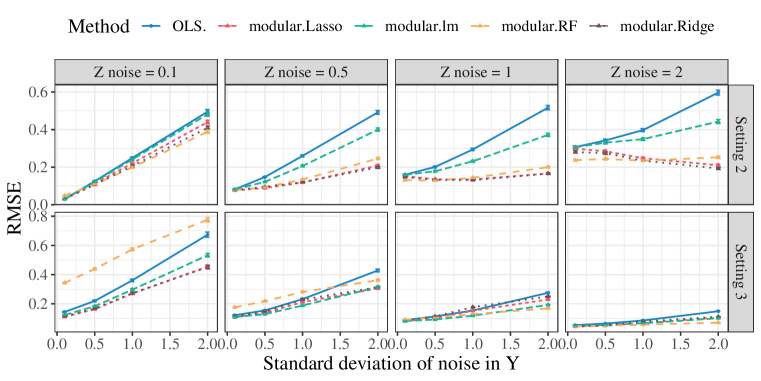
Figure 3: RMSE averaged over $N=1000$ runs with $n=200$. Each column corresponds to a value of $\sigma_{z}$. In each subplot, the $x$-axis (noise strength) equals $\sigma_{y}$, the standard deviation of noise in $Y$. Modular regression achieves smaller estimation error in almost all settings.

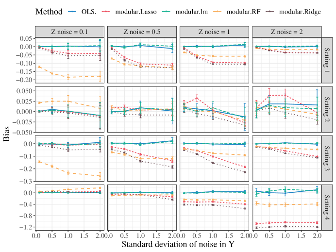
Figure 14: Bias summed over all entries in all settings. Details are otherwise the same as Figure 3. Modular regression incurs a slightly larger bias than OLS when the sub-tasks are learned by flexible machine learning algorithms.

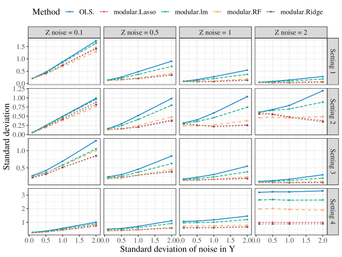
Figure 15: Aggregated SD in all settings. Details are otherwise the same as Figure 3.

Modular regression – no matter which machine learning regressor is used for $\hat{\mu}_{x}$ and $\hat{\mu}_{y}$ – achieves smaller RMSE than the plain OLS in almost all configurations. Modular regression has a larger bias than OLS due to the additional regression (Figure 14, Appendix E), yet much more substantial reduction in standard deviation (Figure 15, Appendix E) in all settings. Also, results from setting 1 confirms Remark 2.5, where the asymptotic variance reduction grows with both $\sigma_{z}$ and $\sigma_{y}$.

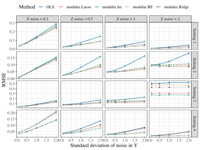
Figure 16: Aggregated RMSE when $n=2000$. Details are otherwise the same as Figure 3.

A noteworthy exception is $\sigma_{z}=0.1$ in setting 3, where the RMSE of modular regression with random forests is worse than that of the OLS estimator. This is because with small sample size ($n=200$) and low noise (hence the uncertainty in $\hat{\theta}_{n}^{\textrm{ols}}$ is very small), the bias introduced by the random forest regression is large compared to the reduction in variance. However, when $\sigma_{z}$ becomes larger, the bias (Figure 14) has a smaller magnitude; this may be because we enter a signal-to-noise ratio regime that favors tree-based approaches. The impact of bias is also less substantial when we increase the sample size. Figure 16 in Appendix E plots the RMSE for estimating $\theta_{1}^{*}$ when $n=2000$, where we see a much better performance of modular regression with random forests. Thus, we recommend using machine learning regressors for larger sample sizes.

We also note that modular regression with linear regression (green) performs better than the plain OLS in all settings (even when the true relation is nonlinear), although it is sometimes outperformed by other modular methods. This phenomenon is universal in our simulation (see Appendix E for RMSE for all entries in all settings), and verifies the relaxed consistency condition we observe after Theorem 2.2. Although this is not a general rule, we still recommend linear regression in practice especially for small sample size. One can also add a few transformed regressors into the linear regression to further adapt to nonlinearity.

Finally, to show the asymptotic behavior of modular regression, in Figure 4 we plot the aggregated RMSE for varying sample sizes $n\in\{200,500,1000,2000\}$ with $\sigma_{z}=0.5$ and $\sigma_{y}=1$ in all settings. Modular regression outperforms OLS in nearly all settings, and linear models (lm, Lasso and Ridge) as base estimators show robust performance. The performance of random forest is less stable for small sample size ($n=200$) in setting 3, hence we recommend using flexible machine learning models with larger sample sizes.

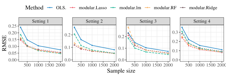
Figure 4: RMSE averaged over $N=1000$ runs for various sample size, and $\sigma_{z}=0.5$, $\sigma_{y}$=1. Modular regression outperforms OLS in all settings, and its performance improves with $n$.

5.2 High-dimensional setting

We now consider two data generating processes in the high-dimensional setting, where the conditional independence structure holds only in one of them. We show that our methods outperform the Lasso in Setting 1 (with conditional independence), and is robust against the violation of conditional independence in Setting 2. Following the preceding notations, $X\in\mathbb{R}^{p_{x}}$ is the covariates available in the prediction phase, while $Z\in\mathbb{R}^{p_{z}}$ is only available for training data, and $Y\in\mathbb{R}$ is the outcome. The data generating processes are visualized in Figure 5.

(a) Setting 1: conditional independence

(b) Setting 2: approximate conditional independence

Figure 5: Illustration of the two data generating processes.

In settting 1, we generate $X\in\mathbb{R}^{p_{x}}$ where each entry is i.i.d. from $N(0,1)$; then we generate $Z=BX+\epsilon_{z}\in\mathbb{R}^{p_{x}}$ with i.i.d. noise $\epsilon_{z}\sim N(0,1)$ given a parameter matrix $B\in\mathbb{R}^{p_{z}\times p_{x}}$. Finally, we generate $Y=Z^{\top}\gamma+\epsilon_{y}$ for i.i.d. random noise $\epsilon_{y}\sim N(0,4)$ and some $\gamma\in\mathbb{R}^{p_{z}}$. To ensure sparsity, we let $B_{ij}=0$ for all $j>s$, such that $X_{j}$’s for $j>s$ are irrelevant for the prediction. Then for each $j\leq s$, we randomly select $2s$ entries in the $j$-th column of $B$ with $B_{ij}=0.25$, the remainings with $B_{ij}=0$. We set $\gamma_{i}=0.5$ for $1\leq i\leq s$, and $\gamma_{i}=0$ for $i>s$. In this way, $Y=X^{\top}\theta^{*}+(\gamma^{\top}\epsilon_{z}+\epsilon_{y})$ where $\theta^{*}=B^{\top}\gamma$, and $X\perp\!\!\!\perp Y{\,|\,}Z$.

In setting 2, we ensure a small subset of covariates in $X$ to have direct impact on $Y$ (the link from $X$ to $Y$ in Figure 5(b)). To be specific, we generate $X$ and $Z=BX+\epsilon_{z}$, where $\{B_{ij}\colon j\leq s\}$ and $\epsilon_{z}$ are the same as setting 1, and generate $Y=Z^{\top}\gamma+X^{\top}\tilde{\gamma}+\epsilon_{y}$ for i.i.d. random noise $\epsilon_{y}\sim N(0,4)$; the direct coefficient $\tilde{\gamma}$ satisfies $\tilde{\gamma}_{i}=0$ for $i\leq s$ and $\sum_{i=1}^{p_{x}}\operatorname{\mathds{1}}\{\tilde{\gamma}_{i}\geq 0\}=5$. In this setting, the high dimensional model $Y=X^{\top}\theta^{*}+(\gamma^{\top}\epsilon_{z}+\epsilon_{y})$ holds with $\theta^{*}=B^{\top}\gamma+\tilde{\gamma}$, but $X\perp\!\!\!\perp Y{\,|\,}Z$ does not hold exactly.

We compare our method in Section 3.1 to the Lasso; to ensure fair comparison, we run the Lasso using our modular method while setting $\hat{f}_{y}(Z_{i}):=Y_{i}$ and $\hat{f}_{x}(Z_{i}):=X_{i}$ for all $i$, so that (11) reduces to the Lasso. We also evaluate an oracle modular regression algorith, that is, we set $\hat{\mu}_{y}:=\mathbb{E}[Y{\,|\,}Z]$ and $\hat{\mu}_{x}:=\mathbb{E}[X_{j}{\,|\,}Z]$ as the ground truth. The regularization parameter $\lambda$ for $\ell_{1}$-penalty is chosen by 5-fold cross validation on the training data for all methods. In our modular regression algorithm, we fit $\hat{\mu}_{x}$ and $\hat{\mu}_{y}$ by ridge regression using the cv.glmnet function from the glmnet R-package (Friedman et al.,, 2010). The procedures are evaluated for $p_{x}=p_{z}=100$ and $s=10$. The training sample is $n=500$ and we evaluate the prediction on $n_{\textrm{test}}=1000$ test samples for a relatively accurate estimate.

5.2.1 Performance under conditional independence

In setting 1 with a well-specified high-dimensional linear model and exact conditional independence $X\perp\!\!\!\perp Y{\,|\,}Z$, we evaluate (i) the parameter estimation error $\|\hat{\theta}_{j}-\theta_{j}^{*}\|_{2}$ where $\hat{\theta}$ is the output of modular regression or the Lasso, as well as (ii) prediction performance: excess risk $\frac{1}{n_{\textrm{test}}}\sum_{i=1}^{n_{\textrm{test}}}(X_{i}^{\top}\hat{\theta}-X_{i}^{\top}\theta^{*})^{2}$ and mean squared error (MSE) $\frac{1}{n_{\textrm{test}}}\sum_{i=1}^{n_{\textrm{test}}}(X_{i}^{\top}\hat{\theta}-Y_{i})^{2}$ on the test samples.

Parameter estimation.

For each $j\in[p_{x}]$, we evaluate the rooted mean squared error (RMSE) $(\hat{\theta}_{j}-\theta^{*}_{j})^{2}$ and bias $|\mathbb{E}[\hat{\theta}_{j}]-\theta_{j}^{*}|$ over $N=100$ replicates, and visualize the RMSE (left) and bias (right) via boxplots in Figure 12.

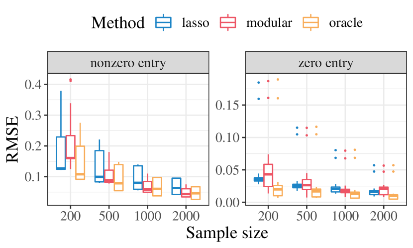
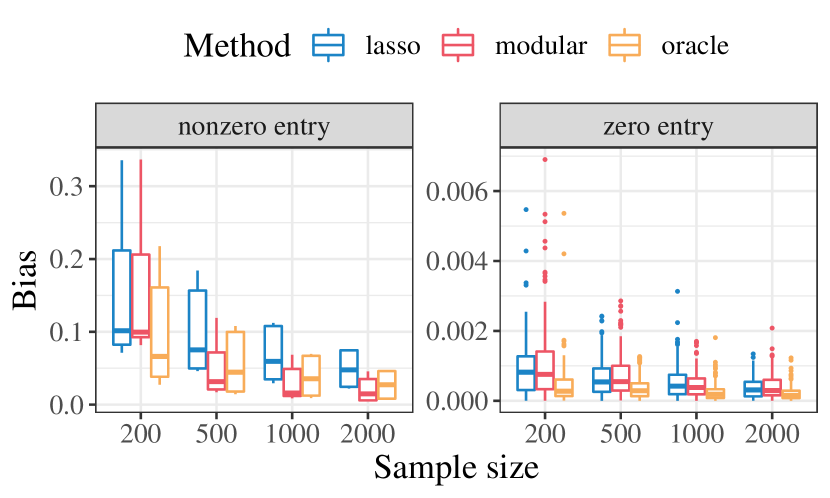
Figure 6: Boxplot of RMSE (left) and bias (right) of $\{\hat{\theta}_{j}\colon j\in[p_{x}]\}$, averaged over all replicates in setting 1, separately for $\theta_{j}^{*}\neq 0$ (nonzero entry) and $\theta_{j}^{*}=0$ (zero entry). The $x$-axis indicates the method to obtain $\hat{\theta}_{j}$. Modular regression achieves smaller RMSE and smaller bias than the Lasso due to a different bias-variance trade-off.

For nonzero entries (the blue boxplots), we observe a significant reduction in RMSE compared to the Lasso under various sample sizes; despite the estimation error in fitting the conditional mean, our method is comparable to its oracle counterpart, even with a smaller overall RMSE (though less stable across entries). This might be due to the instability in cross-fitting with ridge regression or achieving a better bias-variance tradeoff by cross-validation. Also, as $n$ increases, modular regression gets more and more stable. For zero entries, the RMSE are similar across three methods: while the oracle yields lower RMSE than the Lasso, the slight inflation of RMSE in modular prediction might be due to the estimation error of $\hat{\mu}_{x}$ and $\hat{\mu}_{y}$.

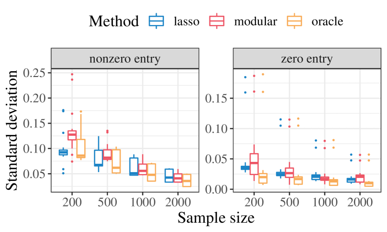
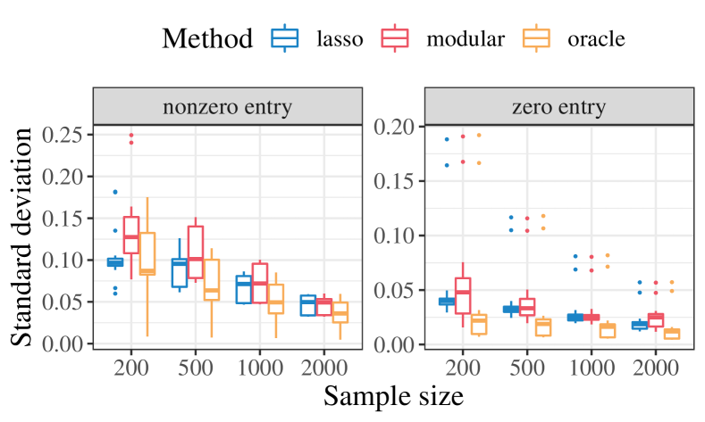
Figure 21: Boxplot of standard deviations for $\{\hat{\theta}_{j}\colon j\in[p_{x}]\}$, averaged over $N=1000$ replicates in setting 1 (left) and setting 2 (right). Other details are the same as Figure 12.

We find that the reduction in RMSE for nonzero entries mainly comes from the reduction in bias, as illustrated by the right panel of Figure 12. This is consistent with our theory in Theorem 3.5: The reduced variance of the proxy $\hat{C}_{\textrm{lm}}$ allows the cross-validation step to choose a model with smaller bias. Due to limited space, we defer the corresponding plot of standard deviations to Figure 21 in Appendix E.

Prediction.

We plot the $N=1000$ excess risks averaged on the test samples for various training sample size $n$ in Figure 7. It shows significant improvement in prediction accuracy of our method compared to plain Lasso; modular regression is slightly inferior to the oracle counterpart but the difference is relatively moderate. The error of modular regression also gets smaller as the sample size increases.

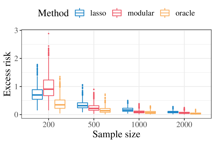
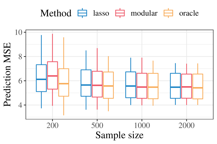
Figure 7: Boxplot of $N=1000$ empirical excess risks $\mathbb{E}[(X_{i}^{\top}\hat{\theta}-X_{i}^{\top}\theta^{*})^{2}]$ and MSEs $\mathbb{E}[(X_{i}^{\top}\hat{\theta}-Y_{i})^{2}]$ in all replicates for setting 1. Modular regression achieves smaller excess risk than the Lasso. The improvement in prediction MSE is less visible due to the irreducible error.

5.2.2 Robustness to approximate conditional independence

In the following, we test the robustness of our method against potential violation of the conditional independence assumption. In setting 2 where the conditional independence only approximately holds, we additionally conduct a structure learning step using Lasso.

We first run a cross-validated Lasso of $Y$ on $(X,Z)$ using the cv.glmnet function (Friedman et al.,, 2010) for model selection; all $X_{j}$ that are selected by this Lasso step is then merged into $Z$. For any selected $X_{j}$, we will skip the regression of $\mathbb{E}[X_{j}{\,|\,}Z]$ and directly set $\hat{f}_{x,j}(Z_{i})=X_{i,j}$ for all training samples. We also evaluate an oracle counterpart which uses the ground truth of the structure and the true conditional expectations for those $X_{j}\perp\!\!\!\perp Y{\,|\,}Z$; we skip the regression for those $X_{j}$ with a direct impact on $Y$, as outlined in Section 3.3.

Figure 8 plots the RMSE (left) and bias (right) of all coefficients $\hat{\theta}_{j}$ with various sample sizes, averaged over $N=1000$ replicates. The plot for standard deviations of $\hat{\theta}_{j}$ is in Figure 21 in Appendix E. We again see an improved RMSE especially for nonzero entries (blue). While the RMSE is less stable across different entries, perhaps because of the additional uncertainty introduced in the structure learning step, it is in general better than plain Lasso and comparable to the oracle. Similar to the previous setting, this reduction of RMSE mainly comes from a reduced bias as shown in the right panel of Figure 8. In general, our method is able to adapt to approximate conditional independence and maintain certain efficiency gain.

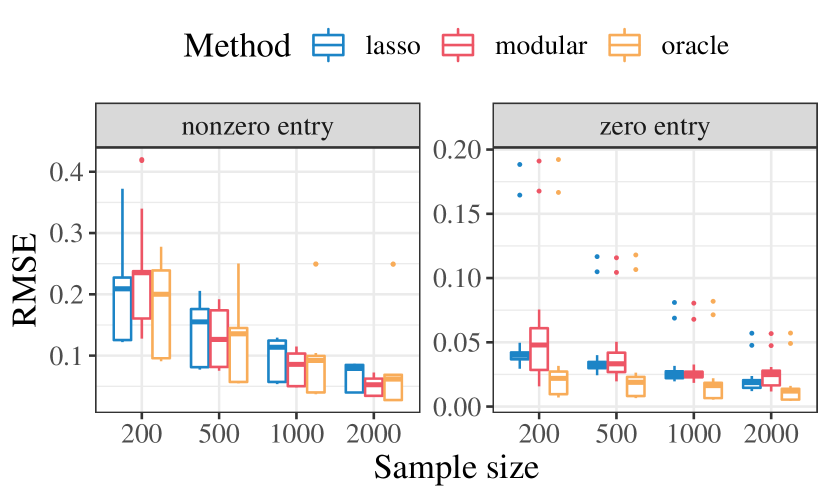
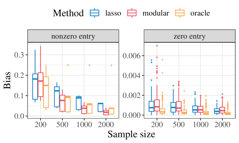
Figure 8: Boxplot of RMSE (left) and bias (right) of $\hat{\theta}_{j}$, $j\in[p_{x}]$, averaged over all replicates, for $\theta_{j}^{*}\neq 0$ (nonzero entry) and $\theta_{j}^{*}=0$ (zero entry) separately. Modular regression achieves smaller estimation RMSE and bias than the Lasso, due to a different bias-variance trade-off.

We summarize the prediction performance in Figure 9. The excess risk of modular prediction lies between that of the oracle counterpart and the Lasso. Still, the relative improvement in terms of prediction MSE is present yet smaller due to the irreducible noise.

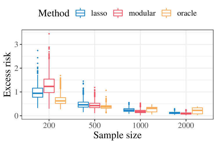
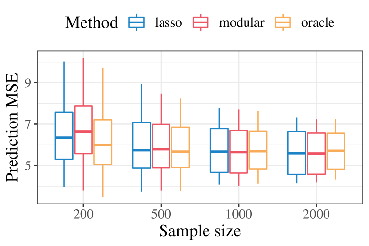
Figure 9: Boxplot of $N=100$ empirical excess risks $(X_{i}^{\top}\hat{\theta}-X_{i}^{\top}\theta^{*})^{2}$ (left) and MSEs $(X_{i}^{\top}\hat{\theta}-Y_{i})^{2}$ (right) in all replicates for setting 2. Modular regression with structure learning achieves smaller prediction excess risk than the Lasso.

6 Real data analysis

6.1 Dataset overview

We apply our method to the English Longitudinal Study of Ageing dataset (Oldfield et al.,, 2021). The waves of data consistently measure several modules of features such as health trajectories, disability and healthy life expectancy, the economic and financial situations, cognition and mental health, etc. We use the Wave 7 and Wave 9 data, collected in 2014 and 2018, respectively, restricted to people who are present in both waves.

We consider predicting the future health outcomes of people based on their current available features. The Wave 7 data is used as covariates. We divide all variables into two categories: health (both mental and physical) and social conditions (including household demographics, financial, work and social situations). After pre-processing through one-hot encoding for categorial and string-valued variables and filtering out some highly imbalanced variables, the health and social categories contain $184$ and $888$ features, respectively. We take the hehelf variable from Wave 9 data as the response $Y$: the reported overall health situation ranging from 1 (excellent) to 5 (poor). We treat the outcome as continuous.

6.2 Real data application

We take the covariates in the social category as $X\in\mathbb{R}^{p_{x}}$ for $p_{x}=888$, and those in the health category as $Z\in\mathbb{R}^{p_{z}}$ for $p_{z}=184$. Our procedure is geared towards settings with high noise. To simulate such a setting, we smooth the discrete response $Y$ by adding i.i.d. noise drawn from $N(0,4)$. The task is to predict $Y$ using $X$, while $Z$ may be available during the training process. This is practical setting where health conditions ($Z$) may be more costly or difficult to evaluate, hence only available in pre-collected data.

We consider a scenario where one only has access to a limited number $n$ of $(X,Y,Z)$ triples as well as $n_{xz}$ observations for $(X,Z)$ and $n_{yz}$ observation for $(Z,Y)$ pairs in the training phase. This mimics a realistic scenario where it is difficult to obtain full observations simultaneously but modular data are more easily accessible. When $n_{xz}=n_{yz}=0$, it reduces to the standard full-observation setting. While it is more difficult to test for conditional independence and the modeling assumptions with limited joint observations, we could still use our framework to merge the individual datasets and improve out-of-sample prediction. We focus on the prediction MSE on the test sample because no ground truth is available. We consider two scenarios:

1. Fixed $n$ and varying $n_{xz}$ and $n_{yz}$. We fix $n=200$, and the number of pair observations varies as $n_{xz}=n_{yz}=n\cdot\rho$ for $\rho\in\{0.5,1,5,10\}$.

2. Fixed $n+n_{xz}+n_{yz}$ and varying proportion. We fix the total sample size $n+n_{xz}+n_{yz}=1000$, while varying the proportion of joint observations by $n=1000\cdot\rho$, $n_{xz}=n_{yz}$ for $\rho\in\{0.05,0.1,0.2,0.5,0.8,1\}$.

We evaluate our modular regression approach outlined in Section 4 that utilizes the partial observations, where we use 2-fold cross-fitting to obtain $\hat{\mu}_{x}$ and $\hat{\mu}_{y}$ from 1) the Lasso using cv.glmnet (10-fold cross-validation), 2) ridge regression using cv.glmnet (10-fold cross-validation), and 3) random forests using grf R-package. The parameter $\lambda$ for $\ell_{1}$-regularization is chosen by 10-fold cross-validation with the 1se criterion, implemented in the same way as that in the cv.glmnet R function, i.e., we selects the largest $\lambda$ within one se of CV error from the smallest CV error. We use the modular regression without structure learning. These implementations are compared to the default Lasso using cv.glmnet fitted over the $(X,Y)$ joint observations, also using 1se criterion for 10-fold validation. Here we omit the results for our methods and the Lasso using the min option (selecting minimum CV error) for cross-validation because the Lasso performs far less stable in this case. The average prediction MSEs over $N=100$ independent runs are in Figure 10.

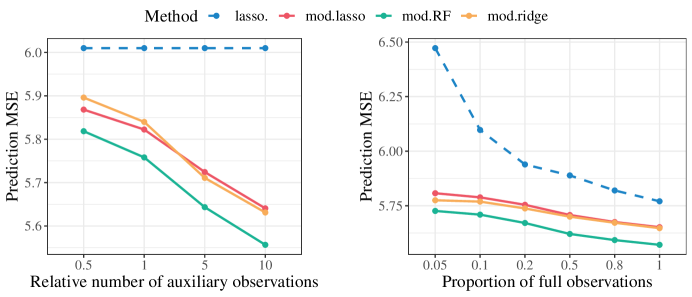
Figure 10: Average prediction MSEs on the test data in settings (i) left and (ii) right. All methods are 1se cross-validated. The $x$-axis represents the value of $\rho$ in both plots. Modular regression with all three base learners substantially reduce the prediction MSE.

The left panel in Figure 10 shows the results for setting (i), where Lasso uses a fixed number of joint observations. As the number of auxiliary observations increases, our modular regression achieves smaller prediction error, showing quite substantial improvement due to incorporating auxiliary observations.

The right panel presents those for setting (ii). Naturally, the performance of the Lasso (blue, dashed line) improves as $\rho$, the proportion of joint observations, increases. Our modular regression, with all of the three regressors, outperforms the Lasso by utilizing auxiliary observations, including $\rho=1$ without missing data. Surprisingly, keeping the total sample size fixed, we do not see much variation in the performance of modular regression (all solid lines) as $\rho$ varies: the performance with only $5\%$ joint observations is comparable to that with more than $50\%$ joint observations. Our method achieves very similar effective sample size as full observations on this dataset. On the other hand, this phenomenon also indicates that we are in a regime where the irreducible error in $Y$ is large compared to the learnable part. In the next part, we are to utilize semi-synthetic data to evaluate the performance of our method in a setting with slighly stronger signal.

6.3 Semi-synthetic data

As discussed in Section 3.4, a naive implementation of our procedure is computationally prohibitive in high-dimensional settings. Thus, in the following, we evaluate the shortcut described in Section 3.4 and compare it with the standard cross-fitting implementation. We keep the choice of $X$ and $Z$ as before, and randomly subsample without replacement the training and test folds, where we observe $(X,Z,Y)$ for $n=1000$ training data, but only $X$ for $n_{\textrm{test}}=1794$ test sample. This is a scenario where only those easier-to-measure social-related covariates are available at the time of prediction, while the pre-collected training data contain both health and social covariates.

Data generating process.

As the signal-to-noise ratio in the original data (for both $(X,Y)$ and $(Z,Y)$ regression) is extremely low, we enhance the signal with the following synthetic data generating process to draw a more informative comparison. We standardize all features using the original dataset, from which we subsample a set of observations aside from the training and test data. On this set, we run the Lasso for $Y$ given $Z$ which finds $13$ nonzero regression coefficients, and for $Y$ given $X$ which finds $12$ nonzero coefficients; we then reorder the features so that $Z_{1:13}$ and $X_{1:12}$ have with nonzero coefficients. For each $j\in\{1,\dots,12\}$, we run a Lasso for $X_{j}$ over $Z_{1:13}$ on this fold, and store all coefficients in the $j$-th column of a matrix $\hat{B}\in\mathbb{R}^{13\times 12}$.

We generate the training and testing data by $Z_{i}=Z_{i}^{\textrm{org}}+\epsilon_{i}^{z}$, where $Z_{i}^{\textrm{org}}$ is the original observation, and $\epsilon_{i}^{z}\sim N(0,\sigma_{z}^{2})$ is independent noise. We then compute $\mu_{x}(Z_{i})=2.5\cdot\hat{B}^{\top}Z_{i,1:13}$, and generate $X_{i,1:12}=\mu_{x}(Z_{i})+\epsilon_{i}^{x}$, where $\epsilon_{i}^{x}\in\mathbb{R}^{12}$ is i.i.d. noise from $N(0,0.25\cdot\mathbf{1}_{12})$ to match the standardized variance in $X$, and $X_{13:p_{x}}$ are obtained by permuting each columns in the (standardized) original data matrices. Finally, we generate $Y_{i}=\mu_{y}(Z_{i})+\epsilon_{i}^{y}$, where $\mu_{y}(Z_{i})=Z_{i}^{\top}\gamma$ where the first $12$ entires in $\gamma\in\mathbb{R}^{p_{z}}$ equals $0.5$ while the others equal to zero, and $\epsilon_{i}^{y}\sim N(0,4)$ is the i.i.d. random noise. This setup ensures $X\perp\!\!\!\perp Y{\,|\,}Z$, but the sparse linear model $\mathbb{E}[Y{\,|\,}X]=X^{\top}\theta^{*}$ does not necessarily hold, and the true parameters $\theta^{*}$ are not available. We thus focus on the prediction performance. We vary the signal-to-noise ratio by setting $\sigma_{z}\in\{1,2\}$.

Methods.

We evaluate two implementations of the modular regression:

1. Cross fitting in Section 3.1. We use two-fold cross-fitting with cross-validated Lasso and ridge regression to form $\hat{\mu}_{x}$ and $\hat{\mu}_{y}$, and then use 10-fold cross-validation to decide the penalty parameter $\lambda$ in (11) by either (a) min: minimal CV error or (b) 1se: the same as the default implementation in cv.glmnet R function which selects the largest $\lambda$ within one se of CV error for stable performance.

2. Projection shortcut in Section 3.4. We use ridge projection with regularization parameters $(\eta_{x},\eta_{y})$ for $\bm{\Pi}_{x},\bm{\Pi}_{y}$, and then run cv.glmnet (with both (a) min and (b) 1se choice of cross-validation) for $X$ and $(\bm{\Pi}_{y}+\bm{\Pi}_{x}-\bm{\Pi}_{x}\bm{\Pi}_{y})Y$, where $(\eta_{x},\eta_{y})$ are chosen by 10-fold cross-validation to minimize CV error.

The above two implementations are compared to two baselines:

1. Oracle modular regression. Set $\hat{\mu}_{x}$ and $\hat{\mu}_{y}$ as ground truth, and then the same as (i).

2. Lasso: Run cv.glmnet on $(X,Y)$ with both (a) min and (b) 1se cross-validation.

Results.

The boxplots for all methods with $N=100$ independent runs are in Figure 11, where we compare the performance under different cross-validation options.

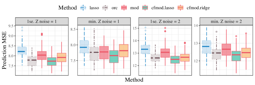
Figure 11: Boxplots of prediction MSEs on the test data. Each subplot summarizes methods with one cross validation option (1se or min) under one value of $\sigma_{z}$. Method stands for the projection shortcut (mod), and cross-fitting with Lasso (cfmod.Lasso) and ridge regression (cfmod.ridge). The Lasso (Lasso) and oracle modular regression (orc) with the same cv option are plotted for comparison. The oracle modular regression substantially reduces MSE; the cross-fitting implementation with Lasso and ridge regression is comparable to the oracle; the projection shortcut is slightly inferior but still improves upon the Lasso.

The patterns across different values of $\sigma_{z}$ are similar. Among the baselines, the Lasso with minimal CV error is more accurate than 1se (see the blue boxplots in the last two columns versus in the first two columns), while the oracle modular regression always achieves smaller prediction MSE than the Lasso with the corresponding CV option (grey).

Our modular regression method performs reasonably well when the conditional mean functions $\mu_{x}(\cdot)$ and $\mu_{y}(\cdot)$ are estimated. When they are estimation by (i) ridge projection shortcut, modular regression with both min (see the last column) and 1se (see the second column) improves upon the Lasso, although it is sometimes less accurate than the oracle. This shows the projection shortcut in Section 3.4 is a reliable alternative to the more computationally intensive cross-fitting approach. When they are estimated by (ii) cross fitting (see the first and third columns), our method improves upon the original Lasso with both Lasso (green) and ridge regression (yellow) as the regressor, and the performance is comparable to the oracle. The Lasso as the regressor is slightly better than the ridge regression; this may be due to the true sparse linear data generating process. In general, for the (ii) implementation, cross-validation with min CV error achieves smaller test MSE than 1se, while the latter sees larger improvement upon the Lasso.

7 Discussion

In this work, we propose the modular regression framework and show that conditional independence structures between variables can be used to decompose statistical tasks into sub-tasks. We develop decomposition techniques for linear models in both low and high dimensional settings. We show that such decomposition can improve efficiency and allow to combine different datasets for a single estimation or prediction task with rigorous statistical guarantees. In practice, the conditional independence conditions for decomposition may be violated, leading to a bias-variance trade-off. We also develop a robust implementation of our method to adapt to potentially more complicated dependence structures.

Looking ahead, statistical tasks that allow for decomposition may go well beyond the cases studied in this work, and the assumptions for decomposition may vary with the nature of the tasks. For instance, in high dimensional graphical models, the edges between variables that indicate independence may be sparse, and conditional independence may not hold exactly for two disjoint sets (e.g., our $X\in\mathbb{R}^{p_{x}}$ and $Z\in\mathbb{R}^{p_{z}}$). In biological applications, there may exist several paths from $X$ to $Y$ rather than being fully mediated by $Z$. The dependence among the features and the response may still be sparse, but additional efforts are needed in order to leverage potential independence structures. In addition, the data fusion technique may be further extended: In practice, one may have access to many auxiliary datasets that cover different sets of features. Developing a framework to systematically combine multiple datasets may also be an interesting direction. Finally, our theoretical results in high dimensions only cover the sparse setting ($p\gg n\gg\log p$ with $s\leq\sqrt{n}$). In this regime, both the LASSO and the modular estimator are consistent, and the role of conditional independence is to lower the variance of residuals. Its role in modern asymptotic regimes such as $p/n\to\rho$ for some fixed $\rho>0$ remains an interesting question.

Appendix A Deferred theoretical results

This section presents the omitted theorem and proof for modular generalized linear regression in Section 2.3.

Assumption A.1.

$\theta^{*}\in\Theta$ for a compact set $\Theta$. Also, $\ell(x,y,\theta)$ is three-times-differentiable and convex in $\theta\in\Theta$. Let $\nabla_{\theta}h(x,\theta)\in\mathbb{R}^{p_{x}}$ denote the first-order derivative of $h(x,\theta)$ in $\theta$, and similarly $\nabla_{\theta}^{2}h(x,\theta)\in\mathbb{R}^{p_{x}\times p_{x}}$ the second-order, and $\nabla_{\theta}^{3}h(x,\theta)\in\mathbb{R}^{p_{x}\times p_{x}\times p_{x}}$ the third-order ones. There exists some $L\colon\mathcal{X}\to\mathbb{R}$ such that $\mathbb{E}[L(X)]<\infty$, and $\|\nabla_{\theta}h(x,\theta)-\nabla_{\theta}h(x,\theta^{\prime})\|\leq L(x)\cdot\|\theta-\theta^{\prime}\|$ for any $\theta,\theta^{\prime}\in\Theta$. Also, there exists some $m\colon\mathcal{X}\times\Theta\to\mathbb{R}$ such that $\mathbb{E}[m(X)]<\infty$ and $\|\nabla_{\theta}^{3}h(x,\theta)-\nabla_{\theta}^{3}h(x,\theta^{\prime})\|_{\textrm{Fro}}\leq m(x)\cdot\|\theta-\theta^{\prime}\|$ for any $\theta,\theta^{\prime}\in\Theta$.

Theorem A.2.

Suppose Assumptions 2.1 and A.1 hold, and $\|\hat{\mu}_{x}^{(k)}-\mu_{x}\|_{L_{2}(\mathbb{P}_{Z})}\|\hat{\mu}_{y}^{(k)}-\mu_{y}\|_{L_{2}(\mathbb{P}_{Z})}=o_{P}(1/\sqrt{n})$ for $k=1,2$. Let $\hat{\theta}_{n}^{\textrm{mod}}$ be the unique minimizer of (10), and $\theta^{*}$ be the unique minimizer of $\mathbb{E}\big{[}\ell(X_{i},Y_{i},\theta^{*})\big{]}$. Let $\mu_{x}(\cdot)=\mathbb{E}[f(X_{i}){\,|\,}Z_{i}=\cdot]$ and $\mu_{y}(\cdot)=\mathbb{E}[Y_{i}{\,|\,}Z_{i}=\cdot]$. Define the influence function $\phi(x,y,z)=\mu_{x}(z)g(y)+f(x)\mu_{y}(z)-\mu_{x}(z)\mu_{y}(z)+\nabla_{\theta}h(x,\theta^{*})$. Then $\sqrt{n}(\hat{\theta}_{n}^{\textrm{mod}}-\theta^{*})\stackrel{{\scriptstyle d}}{{\to}}N(0,\operatorname{\rm Cov}(\phi(X_{i},Y_{i},Z_{i})))$ and $\sqrt{n}(\hat{\theta}_{n}^{\textrm{mod}}-\theta^{*})=\frac{1}{\sqrt{n}}\sum_{i=1}^{n}\phi(X_{i},Y_{i},Z_{i})+o_{P}(1/\sqrt{n})$ as $n\to\infty$. Furthermore, $\phi(X_{i},Y_{i},Z_{i})$ is the efficient influence function for estimating $\theta^{*}$ under the model space obeying Assumption 2.1.

Proof of Theorem A.2.

The proof idea is similar to that of Jin and Rothenhäusler, (2021, Proposition E.2 and Theorem 3.11). Write $\hat{\ell}(X_{i},Y_{i},Z_{i},\theta)=\big{[}\hat{\mu}_{x}(Z_{i})g(Y_{i})+f(X_{i})\hat{\mu}_{y}(Z_{i})-\hat{\mu}_{x}(Z_{i})\hat{\mu}_{y}(Z_{i})\big{]}^{\top}\theta+h(X_{i},\theta)$. We first show that $\hat{\theta}_{n}^{\textrm{mod}}\stackrel{{\scriptstyle P}}{{\to}}\theta^{*}$ as $n\to\infty$. Since the score function $s$ is differentiable and convex in $\theta$, equivalently, $\hat{\theta}_{n}^{\textrm{mod}}\in\Theta$ is the unique solution to

$$\hat{L}_{n}^{\textrm{mod}}(\theta) :=\frac{1}{n}\sum_{i=1}^{n}\big{[}\hat{\mu}_{x}(Z_{i})g(Y_{i})+f(X_{i})\hat{\mu}_{y}(Z_{i})-\hat{\mu}_{x}(Z_{i})\hat{\mu}_{y}(Z_{i})+\nabla_{\theta}h(X_{i},\theta)\big{]}=0,$$

while the population parameter $\theta^{*}$ is the unique solution to

$$L(\theta):=\mathbb{E}\big{[}\nabla_{\theta}\ell(X_{i},Y_{i},\theta)\big{]}=\mathbb{E}\big{[}g(Y_{i})f(X_{i})+\nabla_{\theta}h(X_{i},\theta)\big{]}=0.$$

We also define the empirical score at any $\theta\in\Theta$ as

$$\hat{L}_{n}(\theta)=\frac{1}{n}\sum_{i=1}^{n}\big{[}g(Y_{i})f(X_{i})+\nabla_{\theta}h(X_{i},\theta)\big{]}.$$

Then for any fixed $\theta\in\Theta$, we note that

$$\hat{L}_{n}^{\textrm{mod}}(\theta)-\hat{L}_{n}(\theta)=\frac{1}{n}\sum_{i=1}^{n}\big{[}\hat{\mu}_{x}(Z_{i})g(Y_{i})+f(X_{i})\hat{\mu}_{y}(Z_{i})-\hat{\mu}_{x}(Z_{i})\hat{\mu}_{y}(Z_{i})-g(Y_{i})f(X_{i})\big{]}$$

$$=\frac{1}{n}\sum_{k=1}^{2}\sum_{i\in\mathcal{I}_{k}}\big{[}\hat{\mu}^{(k)}_{x}(Z_{i})g(Y_{i})+f(X_{i})\hat{\mu}^{(k)}_{y}(Z_{i})-\hat{\mu}^{(k)}_{x}(Z_{i})\hat{\mu}^{(k)}_{y}(Z_{i})-g(Y_{i})f(X_{i})\big{]}.$$

Similar to the proof of Theorem 2.2 (see equation (22)), under the given consistency condition for $\hat{\mu}_{x}^{(k)}$ and $\hat{\mu}_{y}^{(k)}$, we know $\sup_{\theta\in\Theta}\big{|}\hat{L}_{n}^{\textrm{mod}}(\theta)-\hat{L}_{n}(\theta)\big{|}=o_{P}(1)$. Furthermore, the law of large numbers implies $\frac{1}{n}\sum_{i=1}^{n}|\hat{L}_{n}(\theta)-L(\theta)|=o_{P}(1)$ for any fixed $\theta\in\Theta$. Therefore, $\big{|}\hat{L}_{n}^{\textrm{mod}}(\theta)-{L}(\theta)\big{|}=o_{P}(1)$ for any fixed $\theta\in\Theta$.

Since $\Theta$ is compact and $\nabla_{\theta}h(x,\theta)$ is $L(x)$-Lipschitz in $\theta\in\Theta$ for any $x\in\mathcal{X}$, we know that for any $\theta,\theta^{\prime}\in\Theta$, by the triangular inequality,

$$\big{|}\hat{L}_{n}(\theta)-\hat{L}_{n}(\theta^{\prime})\big{|}\leq\frac{1}{n}\sum_{i=1}^{n}L(X_{i})\cdot\|\theta-\theta^{\prime}\|,$$

where $\frac{1}{n}\sum_{i=1}^{n}L(X_{i})=O_{P}(1)$ since $\mathbb{E}[L(X)]<\infty$. Thus, for any fixed $\epsilon>0$, there exists a finite subset $\{\theta_{1},\dots,\theta_{N_{\epsilon}}\}$ of $\Theta$ such that $\sup_{\theta}\inf_{1\leq i\leq N_{\epsilon}}|\hat{L}_{n}(\theta)-\hat{L}_{n}(\theta_{i})|\leq\epsilon$. Similar arguments applied to $L(\theta)$, together with the convergence, implies $\sup_{\theta\in\Theta}|\hat{L}_{n}(\theta)-L(\theta)|=o_{P}(1)$. Thus we have $\sup_{\theta\in\Theta}|\hat{L}_{n}^{\textrm{mod}}(\theta)-L(\theta)|=o_{P}(1)$. On the other hand, the compactness of $\Theta$ and the uniqueness of $\theta^{*}$ as a solution to $L(\theta)=0$ implies the well-separatedness condition (c.f. Van der Vaart, (2000, Theorem 5.9)): for any $\epsilon>0$, one could find some $\delta>0$ such that $\inf_{\theta\colon\|\theta-\theta^{*}\|\geq\delta}\big{|}L(\theta)\big{|}>2\epsilon$. Since $\sup_{\theta\in\Theta}|\hat{L}_{n}^{\textrm{mod}}(\theta)-L(\theta)|=o_{P}(1)$, for any fixed $\epsilon>0$, one could find some $\delta>0$ such that for $n$ sufficiently large, $\mathbb{P}\big{(}\inf_{\theta\colon\|\theta-\theta^{*}\|\geq\delta}\frac{1}{n}|\hat{L}_{n}^{\textrm{mod}}(\theta)|>\epsilon\big{)}\geq 1-\epsilon$, i.e., $\mathbb{P}(\|\hat{\theta}_{n}^{\textrm{mod}}-\theta^{*}\|\leq\delta)\geq 1-\epsilon$. This proves $\hat{\theta}_{n}^{\textrm{mod}}-\theta^{*}=o_{P}(1)$.

We now proceed to show the asymptotic normality of $\hat{\theta}_{n}^{\textrm{mod}}$. Recall that $\hat{L}_{n}^{\textrm{mod}}(\hat{\theta}_{n}^{\textrm{mod}})=0$. Taylor expansion around $\theta^{*}$ then gives

$$0=\hat{L}_{n}^{\textrm{mod}}(\theta^{*})+\nabla_{\theta}\hat{L}_{n}^{\textrm{mod}}(\theta^{*})(\hat{\theta}_{n}^{\textrm{mod}}-\theta^{*})+1/2\cdot(\hat{\theta}_{n}^{\textrm{mod}}-\theta^{*})\nabla_{\theta}^{2}\hat{L}_{n}^{\textrm{mod}}(\tilde{\theta}_{n})(\hat{\theta}_{n}^{\textrm{mod}}-\theta^{*})$$ (20)

for some $\tilde{\theta}_{n}$ that lies on the segment between $\hat{\theta}_{n}^{\textrm{mod}}$ and $\theta^{*}$, which implies $\tilde{\theta}_{n}=\theta^{*}+o_{P}(1)$. Here $\nabla_{\theta}\hat{L}_{n}^{\textrm{mod}}\in\mathbb{R}^{p_{x}\times p_{x}}$ and $\nabla_{\theta}^{2}\hat{L}_{n}^{\textrm{mod}}\in\mathbb{R}^{p_{x}\times p_{x}\times p_{x}}$ are second and third order derivative of $\sum_{i=1}^{n}\hat{\ell}(X_{i},Y_{i},Z_{i},\theta)$. By definition

$$\nabla_{\theta}\hat{L}_{n}^{\textrm{mod}}(\theta)=\frac{1}{n}\sum_{i=1}^{n}\nabla_{\theta}^{2}h(X_{i},\theta),\quad\nabla_{\theta}^{2}\hat{L}_{n}^{\textrm{mod}}(\theta)=\frac{1}{n}\sum_{i=1}^{n}\nabla_{\theta}^{3}h(X_{i},\theta).$$

The law of large numbers imply $\nabla_{\theta}\hat{L}_{n}^{\textrm{mod}}(\theta^{*})=\mathbb{E}[\nabla_{\theta}^{2}h(X_{i},\theta^{*})]+o_{P}(1)$ where $o_{P}(1)$ means a matrix whose every entry is $o_{P}(1)$, hence $\nabla_{\theta}\hat{L}_{n}^{\textrm{mod}}(\theta^{*})$ is invertible for sufficiently large $n$. Also, by the Lipschitz condition of $\nabla_{\theta}^{3}h(x,\theta)$ and the triangular inequality, we have

$$\big{|}\nabla_{\theta}^{2}\hat{L}_{n}^{\textrm{mod}}(\theta^{*})-\nabla_{\theta}^{2}\hat{L}_{n}^{\textrm{mod}}(\tilde{\theta}_{n})\big{|}\leq\frac{1}{n}\sum_{i=1}^{n}m(X_{i})\|\theta^{*}-\tilde{\theta}_{n}\|=o_{P}(1)$$

since $\mathbb{E}[m(X_{i})]<\infty$. Hence $\nabla_{\theta}^{2}\hat{L}_{n}^{\textrm{mod}}(\tilde{\theta}_{n})=O_{P}(1)$. Returning to (20), we have

$$0 =\hat{L}_{n}^{\textrm{mod}}(\theta^{*})+\big{\{}\mathbb{E}[\nabla_{\theta}^{2}h(X_{i},\theta^{*})]+o_{P}(1)\big{\}}(\hat{\theta}_{n}^{\textrm{mod}}-\theta^{*})+O_{P}\big{(}\|\hat{\theta}_{n}^{\textrm{mod}}-\theta^{*}\|^{2}\big{)}$$

$$=\hat{L}_{n}^{\textrm{mod}}(\theta^{*})+\big{\{}\mathbb{E}[\nabla_{\theta}^{2}h(X_{i},\theta^{*})]+o_{P}(1)\big{\}}(\hat{\theta}_{n}^{\textrm{mod}}-\theta^{*}),$$

and thus

$$\hat{\theta}_{n}^{\textrm{mod}}-\theta^{*}=\mathbb{E}\big{[}\nabla_{\theta}^{2}h(X_{i},\theta^{*})\big{]}^{-1}\hat{L}_{n}^{\textrm{mod}}(\theta^{*})+o_{P}\big{(}\hat{L}_{n}^{\textrm{mod}}(\theta^{*})\big{)}.$$ (21)

Finally, we note that under the consitency condition of $\hat{\mu}_{x}^{(k)}$ and $\hat{\mu}_{y}^{(k)}$, similar to the proof of Theorem 2.2, one could show that

$$\hat{L}_{n}^{\textrm{mod}}(\theta^{*}) =\frac{1}{n}\sum_{i=1}^{n}\big{[}{\mu}_{x}(Z_{i})g(Y_{i})+f(X_{i}){\mu}_{y}(Z_{i})-{\mu}_{x}(Z_{i}){\mu}_{y}(Z_{i})+\nabla_{\theta}h(X_{i},\theta^{*})\big{]}+o_{P}(1/\sqrt{n}).$$

Because $X\perp\!\!\!\perp Y{\,|\,}Z$, we have $\mathbb{E}\big{[}{\mu}_{x}(Z_{i})g(Y_{i})+f(X_{i}){\mu}_{y}(Z_{i})-{\mu}_{x}(Z_{i}){\mu}_{y}(Z_{i})+\nabla_{\theta}h(X_{i},\theta^{*})\big{]}=\mathbb{E}[\nabla_{\theta}s(X_{i},Y_{i},\theta^{*})]=0$, hence $\hat{L}_{n}^{\textrm{mod}}(\theta^{*})=O_{P}(1/\sqrt{n})$, which, combined with (21), implies

$$\hat{\theta}_{n}^{\textrm{mod}}-\theta^{*}=\mathbb{E}\big{[}\nabla_{\theta}^{2}h(X_{i},\theta^{*})\big{]}^{-1}\hat{L}_{n}^{\textrm{mod}}(\theta^{*})+o_{P}(1/\sqrt{n})$$

$$=\frac{1}{n}\sum_{i=1}^{n}\mathbb{E}\big{[}\nabla_{\theta}^{2}h(X_{i},\theta^{*})\big{]}^{-1}\big{[}{\mu}_{x}(Z_{i})g(Y_{i})+f(X_{i}){\mu}_{y}(Z_{i})-{\mu}_{x}(Z_{i}){\mu}_{y}(Z_{i})+\nabla_{\theta}h(X_{i},\theta^{*})\big{]}+o_{P}(1/\sqrt{n}).$$

We thus complete the proof of the asymptotic expansion of $\hat{\theta}_{n}^{\textrm{mod}}$ in Theorem A.2.

Finally, the efficient influence function for estimating $\theta^{*}$ among all models obeying $X\perp\!\!\!\perp Y{\,|\,}Z$ can be obtained by, similar to Theorem 2.2, projecting the influence function of $\hat{\theta}_{n}^{\textrm{ml}}$ onto the tangent space ${\mathcal{T}}={\mathcal{T}}_{1}\oplus{\mathcal{T}}_{2}\oplus{\mathcal{T}}_{3}$ where ${\mathcal{T}}_{j}$ is defined as in (C.1). Standard M-estimator theory (Van der Vaart,, 2000) gives $\hat{\theta}_{n}^{\textrm{ml}}-\theta^{*}=\frac{1}{n}\sum_{i=1}^{n}\phi^{\textrm{ml}}(X_{i},Y_{i})+o_{P}(1/\sqrt{n})$ where

$$\phi^{\textrm{ml}}(x,y)=\mathbb{E}\big{[}\nabla_{\theta}^{2}h(X_{i},\theta^{*})\big{]}^{-1}\big{[}g(Y_{i})f(X_{i})+\nabla_{\theta}h(X_{i},\theta^{*})\big{]}.$$

The projection follows exactly the same idea as Theorem A.2 and one could see $\phi$ is the efficient influence function. We thus complete the proof of Theorem A.2. ∎

Appendix B Deferred discussion

B.1 Deferred discussion for Remark 2.6

Below, we provide a (simplified) finite-sample analysis of the two methods: (i) OLS, and (ii) modular OLS, where $Y{\,|\,}Z$ and $X{\,|\,}Z$ are estimated using OLS, under a joint Gaussian distribution. This discussion elaborates on the computation details for Remark 2.6.

To be more specific, the cross-term $C=\mathbb{E}[XY]$ is estimated via $\hat{C}_{\textrm{ols}}:=\frac{1}{n}\sum_{i=1}^{n}X_{i}Y_{i}$ or $\hat{C}_{\textrm{mod}}=\frac{1}{n}\sum_{i=1}^{n}Y_{i}\hat{\mu}_{x}(Z_{i})+X_{i}\hat{\mu}_{y}(Z_{i})-\hat{\mu}_{x}(Z_{i})\hat{\mu}_{y}(Z_{i})$. Hereafter, we override the notations and use $X,Y,Z$ to denote data vectors in $\mathbb{R}^{n}$. With OLS regression, we have $\hat{\mu}_{x}(z)=\hat{\theta}_{x}^{\top}z$, where $\hat{\theta}_{x}=(Z^{\top}Z)^{-1}Z^{\top}X$ is the fitted OLS coefficient of $X$ on $Z$, and similarly $\hat{\mu}_{y}(z)=\hat{\theta}_{y}^{\top}z$, where $\hat{\theta}_{y}=(Z^{\top}Z)^{-1}Z^{\top}Y$. Then, our modular estimator for the cross-term $\hat{C}_{\textrm{lm}}$ is

$$\hat{C}_{\textrm{mod}}=\frac{1}{n}\sum_{i=1}^{n}Y_{i}Z_{i}^{\top}\hat{\theta}_{x}+X_{i}Z_{i}^{\top}\hat{\theta}_{y}-Z_{i}^{\top}\hat{\theta}_{x}Z_{i}^{\top}\hat{\theta}_{y}$$

$$=\frac{1}{n}\Big{(}Y^{\top}Z\hat{\theta}_{x}+X^{\top}Z\hat{\theta}_{y}-\hat{\theta}_{x}^{\top}Z^{\top}Z\hat{\theta}_{y}\Big{)}$$

$$=\frac{1}{n}\Big{(}Y^{\top}Z(Z^{\top}Z)^{-1}Z^{\top}X+X^{\top}Z(Z^{\top}Z)^{-1}Z^{\top}Y-X^{\top}Z(Z^{\top}Z)^{-1}Z^{\top}Z(Z^{\top}Z)^{-1}Z^{\top}Y\Big{)}$$

$$=\frac{1}{n}\Big{(}Y^{\top}Z(Z^{\top}Z)^{-1}Z^{\top}X+X^{\top}Z(Z^{\top}Z)^{-1}Z^{\top}Y-X^{\top}Z(Z^{\top}Z)^{-1}Z^{\top}Y\Big{)}$$

$$=\frac{1}{n}Y^{\top}Z(Z^{\top}Z)^{-1}Z^{\top}X,$$

where the third row plugs in the definition of $\hat{\theta}_{x}$ and $\hat{\theta}_{y}$, and the last line uses the fact that $Y^{\top}Z(Z^{\top}Z)^{-1}Z^{\top}X=X^{\top}Z(Z^{\top}Z)^{-1}Z^{\top}Y$. The two estimators are $\hat{\theta}_{n}^{\textrm{ols}}=(X^{\top}X/n)^{-1}\hat{C}_{\textrm{ols}}$, and $\hat{\theta}_{n}^{\textrm{mod}}=(X^{\top}X/n)^{-1}\hat{C}_{\textrm{mod}}$, respectively.

Suppose $X,Y,Z$ are all one-dimensional and jointly Gaussian. Then, there exists a decomposition $X=\alpha Z+\epsilon_{x}$ and $Y=\beta Z+\epsilon_{y}$, where conditional on $Z$, $\epsilon_{x}$ and $\epsilon_{y}$ are normal with mean zero and mutually independent under the assumption $X\perp\!\!\!\perp Y{\,|\,}Z$. We further assume $\epsilon_{x}{\,|\,}Z\sim N(0,\sigma_{x}^{2})$ and $\epsilon_{y}{\,|\,}Z\sim N(0,\sigma_{y}^{2})$. Then, the population OLS parameter is $\theta^{*}=\alpha\beta/(\alpha^{2}+\sigma_{x}^{2})$. Also,

$$\mathbb{E}[\hat{\theta}_{n}^{\textrm{mod}}]=\mathbb{E}\bigg{[}\mathbb{E}\bigg{[}\frac{Y^{\top}Z\cdot Z^{\top}X}{X^{\top}X\cdot Z^{\top}Z}\,\bigg{|}\,X,Z\bigg{]}\bigg{]}=\beta\mathbb{E}\bigg{[}\frac{Z^{\top}Z\cdot Z^{\top}X}{X^{\top}X\cdot Z^{\top}Z}\bigg{]}=\beta\mathbb{E}\bigg{[}\mathbb{E}\bigg{[}\frac{Z^{\top}X}{X^{\top}X}\,\bigg{|}\,X\bigg{]}\bigg{]},$$

where we repeatedly used the tower property. Using the joint Gaussianity of $(X,Z)$, we know that $\mathbb{E}[Z{\,|\,}X]=\frac{\alpha}{\alpha^{2}+\sigma_{x}^{2}}X$, which gives $\mathbb{E}[\hat{\theta}_{n}^{\textrm{mod}}]=\theta^{*}$, hence $\hat{\theta}_{n}^{\textrm{mod}}$ is unbiased. Similarly one can show $\hat{\theta}_{n}^{\textrm{ols}}$ is unbiased.

We now study the variances of the two estimators. By the decomposition of variance,

$$\operatorname{{\rm Var}}(\hat{\theta}_{n}^{\textrm{mod}}) =\mathbb{E}[\operatorname{{\rm Var}}(\hat{\theta}_{n}^{\textrm{mod}}{\,|\,}X,Z)]+\operatorname{{\rm Var}}(\mathbb{E}[\hat{\theta}_{n}^{\textrm{mod}}{\,|\,}X,Z])$$

$$=\mathbb{E}\bigg{[}\frac{(Z^{\top}X)^{2}\sum_{i=1}^{n}Z_{i}^{2}\sigma_{y}^{2}}{(X^{\top}X\cdot Z^{\top}Z)^{2}}\bigg{]}+\operatorname{{\rm Var}}\bigg{(}\frac{\beta Z^{\top}X}{X^{\top}X}\bigg{)}$$

$$=\sigma_{y}^{2}\mathbb{E}\bigg{[}\frac{(Z^{\top}X)^{2}}{(X^{\top}X)^{2}\cdot Z^{\top}Z}\bigg{]}+\beta^{2}\operatorname{{\rm Var}}\bigg{(}\frac{Z^{\top}X}{X^{\top}X}\bigg{)}.$$

Similarly, using the fact that $Y\perp\!\!\!\perp X{\,|\,}Z$,

$$\operatorname{{\rm Var}}(\hat{\theta}_{n}^{\textrm{ols}}) =\mathbb{E}[\operatorname{{\rm Var}}(\hat{\theta}_{n}^{\textrm{ols}}{\,|\,}X,Z)]+\operatorname{{\rm Var}}(\mathbb{E}[\hat{\theta}_{n}^{\textrm{ols}}{\,|\,}X,Z])$$

$$=\mathbb{E}\bigg{[}\frac{\sum_{i=1}^{n}X_{i}^{2}\sigma_{y}^{2}}{(X^{\top}X)^{2}}\bigg{]}+\operatorname{{\rm Var}}\bigg{(}\frac{\beta Z^{\top}X}{X^{\top}X}\bigg{)}=\sigma_{y}^{2}\mathbb{E}\bigg{[}\frac{1}{X^{\top}X}\bigg{]}+\beta^{2}\operatorname{{\rm Var}}\bigg{(}\frac{Z^{\top}X}{X^{\top}X}\bigg{)}.$$

This gives (using $X=\alpha Z+\epsilon_{x}$)

$$\operatorname{{\rm Var}}(\hat{\theta}_{n}^{\textrm{ols}})-\operatorname{{\rm Var}}(\hat{\theta}_{n}^{\textrm{mod}}) =\sigma_{y}^{2}\mathbb{E}\bigg{[}\frac{Z^{\top}Z\cdot X^{\top}X-(Z^{\top}X)^{2}}{(X^{\top}X)^{2}\cdot Z^{\top}Z}\bigg{]}$$

$$=\sigma_{y}^{2}\mathbb{E}\bigg{[}\frac{Z^{\top}Z\cdot\epsilon_{x}^{\top}\epsilon_{x}-(Z^{\top}\epsilon_{x})^{2}}{(X^{\top}X)^{2}\cdot Z^{\top}Z}\bigg{]}\geq 0$$

by the Cauchy-Schwarz inequality (it is a strict inequality as long as $\epsilon_{x}$ is not deterministic given $Z$). That is, in finite sample, both estimators are unbiased, while the modular estimator is non-inferior to OLS in terms of variance.

B.2 Deferred discussion on alternative estimators

In this part, we elaborate our discussion on the alternative estimators in Remark 2.3. In the following, we consider using powerful machine learning algorithms (black-boxes) to estimate the nuisance components $\mu_{x}$ and $\mu_{y}$. They may achieve a smaller MSE than the OLS estimator, potentially at the cost of some bias. The semiparametric efficiency in Theorem 2 of our manuscript does not account for such cases. In the following, we conduct additional experiments to explore this regime.

Surprisingly, we found that (a) outcome regression can achieve a smaller MSE than the OLS, and that (b) orthogonal regression is often less accurate. Nonetheless, our modular estimator often achieves the smallest (or nearly smallest) MSE.

In Figure 12, we show results for OR (standing for outcome regression), PS (standing for orthogonal regression), OLS, and modular regression under several simple data-generating processes, where the true regression functions only involve $\leq 4$ entries. We vary the signal-to-noise ratio and the smoothness of the underlying regression functions across settings. We label the first row as (a-c), and the second as (d-f). Settings (a) and (b) has $Z\in\mathbb{R}^{p_{20}}$, and the true regression functions are a combination of indicator functions and smooth exponential functions. Setting (c) involves a larger number of combinations of polynomial and exponential functions for $Z\in\mathbb{R}^{20}$. Settings (d) and (e) adds a term $\sqrt{n}Z_{3}Z_{4}$ to fixed regression functions that only involve the first 4 variables in $Z\in\mathbb{R}^{100}$. Setting (f) uses a similar model as (a-c) but kept $Z\in\mathbb{R}^{100}$. (d-f) has larger noise level. We omit details on the regression functions for brevity.

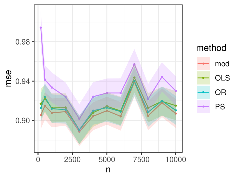
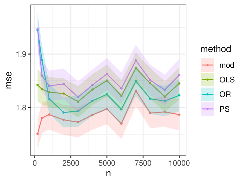
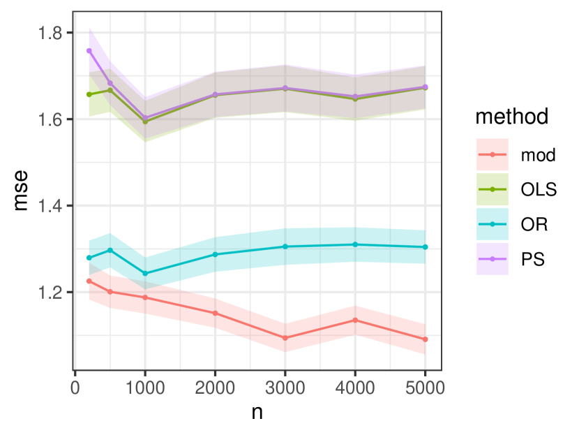
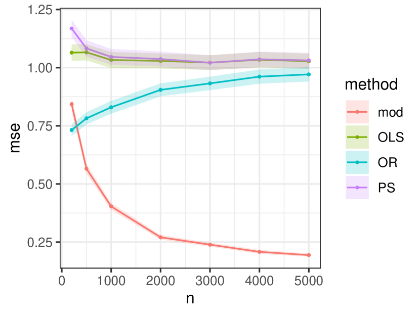
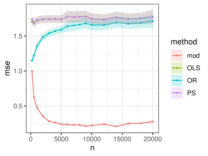
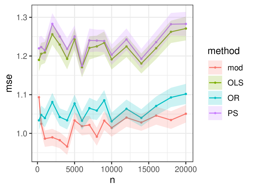
Figure 12: Root-mean-squared error scaled by $\sqrt{n}$, for all methods under different sample sizes.

We see that OR often performs better in terms of MSE; we conjecture that this is because the tuned ML regressor achieves a good bias-variance tradeoff. The PS approach is usually not very accurate, but surprisingly comparable to OLS. A potential explanation is that we are in the regime of “undersmoothing”, i.e., the ML estimator has extremely small bias but larger variance, so that it is still possible to achieve good performance for both OR and PS approaches. Finally, however, the modular estimator always performs the best across all settings; we conjecture that this is because it takes the best of the two worlds, powerful prediction machines and rigorous debiasing ideas from semiparametric statistics.

B.3 Discussion on the estimation of $\hat{J}$

Here, we discuss the conditions for estimating $\hat{J}$ and its compatibility with Assumption 3.4.

Consistent estimation of $J$ require strong conditions such as the beta-min conditions or the irrepresentable conditions Zhao and Yu, (2006). However, it is also known that Lasso selects a superset of “relevant” features, i.e., entries whose coefficient is sufficently bounded away from zero (roughly, these are coefficients with absolute values larger than $O(\sqrt{s_{0}/n\cdot\log p}$, where $s_{0}$ is the number of nonzero coefficients) under less restrictive eigenvalue conditions of the covariates $X$ (see, e.g., Van De Geer and Bühlmann, (2009); Bühlmann and Van De Geer, (2011); Bühlmann, (2010)). When the entries in $J$ are sufficiently large, then a superset of $J$ can be recovered with high probability. Otherwise, entries with small coefficients would not incur too much bias in this process.

On the other hand, consistency estimation of $J$ typically asks for $\log p_{z}/\sqrt{n}\to 0$, while Assumption 3.4 asks for $\|\hat{\mu}_{x,z}^{(k)}(\cdot)-\mu_{x,z}^{(k)}(\cdot)\|_{L_{2}(\mathbb{P}_{Z})}\preceq n^{-1/4}$. When the regression function $\hat{\mu}_{x,z}$ is obtained from high-dimensional regression such as the Lasso, the convergence rate is typically $\sqrt{s_{x,z}\log p_{z}/n}$, where $s_{x,z}$ is the sparsity level for an entry in $X$ over $Z$. These conditions on $p_{z}$ are typically compatible for the two parts (as they are both satisfied for relatively small $p_{z}$). For example, if the sparsity $s_{x,z}$ is bounded, and $\log p_{z}=o(n^{1/4})$, then both conditions are satisfied.

Appendix C Technical proofs

C.1 Proof of Theorem 2.2

Proof of Theorem 2.2.

Recall that $\theta^{*}$ is the least-squares estimator $\theta^{*}=\mathop{\mathrm{argmin}}_{\theta\in\mathbb{R}^{p_{x}}}\mathbb{E}[(Y-X^{\top}\theta)^{2}]$. The estimation equation gives

$$\hat{\theta}_{n}^{\textrm{ols}}-\theta^{*} =\Big{(}\sum_{i=1}^{n}X_{i}X_{i}^{\top}\Big{)}^{-1}\sum_{i=1}^{n}X_{i}Y_{i}-\theta^{*}=\Big{(}\frac{1}{n}\sum_{i=1}^{n}X_{i}X_{i}^{\top}\Big{)}^{-1}\frac{1}{n}\sum_{i=1}^{n}X_{i}(Y_{i}-X_{i}^{\top}\theta^{*}).$$

Since $X_{i}(Y_{i}-X_{i}^{\top}\theta^{*})$ has finite second moment and we know $\mathbb{E}[X(Y-X^{\top}\theta^{*})]=0$ by the optimality of $\theta^{*}$, we have $\frac{1}{n}\sum_{i=1}^{n}X_{i}(Y_{i}-X_{i}^{\top}\theta^{*})=O_{P}(1/\sqrt{n})$, where $O_{P}(1/\sqrt{n})$ represents a random vector whose each entry is $O_{P}(1/\sqrt{n})$. Since $X_{i}X_{i}^{\top}$ has finite expectation $\mathbb{E}[XX^{\top}]\succ 0$, we have

$$\Big{(}\frac{1}{n}\sum_{i=1}^{n}X_{i}X_{i}^{\top}\Big{)}^{-1}=\Big{(}\mathbb{E}[XX^{\top}]+o_{P}(1)\Big{)}^{-1}=\big{(}\mathbb{E}[XX^{\top}]\big{)}^{-1}+o_{P}(1),$$

where $o_{P}(1)$ stands for a random matrix whose all entries converge in probability to zero. We thus have

$$\hat{\theta}_{n}^{\textrm{ols}}-\theta^{*} =\Big{(}\big{(}\mathbb{E}[XX^{\top}]\big{)}^{-1}+o_{P}(1)\Big{)}\frac{1}{n}\sum_{i=1}^{n}X_{i}(Y_{i}-X_{i}^{\top}\theta^{*})$$

$$=\frac{1}{n}\sum_{i=1}^{n}\big{(}\mathbb{E}[XX^{\top}]\big{)}^{-1}X_{i}(Y_{i}-X_{i}^{\top}\theta^{*})+o_{P}(1)\times O_{P}(1/\sqrt{n})$$

$$=\frac{1}{n}\sum_{i=1}^{n}\phi^{\textrm{ols}}(X_{i},Y_{i})+o_{P}(1/\sqrt{n}),$$

where $\phi^{\textrm{ols}}(x,y)=\mathbb{E}[XX^{\top}]^{-1}x(y-x^{\top}\theta^{*}).$ For our modular estimator, we first note the closed form solution

$$\hat{\theta}_{n}^{\textrm{mod}}-\theta^{*}=\Big{(}\sum_{i=1}^{n}X_{i}X_{i}^{\top}\Big{)}^{-1}\sum_{i=1}^{n}C_{i}-\theta^{*}=\Big{(}\sum_{i=1}^{n}X_{i}X_{i}^{\top}\Big{)}^{-1}\sum_{i=1}^{n}\big{(}C_{i}-X_{i}X_{i}^{\top}\theta^{*}\big{)}.$$

We now show that under the conditions in Theorem 2.2, one has

$$\frac{1}{n}\sum_{i=1}^{n}\big{(}C_{i}-X_{i}X_{i}^{\top}\theta^{*}\big{)}=\frac{1}{n}\sum_{i=1}^{n}\big{(}C_{i}^{*}-X_{i}X_{i}^{\top}\theta^{*}\big{)}+o_{P}(1/\sqrt{n}),$$ (22)

where $C_{i}^{*}=X_{i}\mu_{y}(Z_{i})+\mu_{x}(Z_{i})Y_{i}-\mu_{x}(Z_{i})\mu_{y}(Z_{i})$. To see this, by rearranging the terms, we have $\frac{1}{n}\sum_{i=1}^{n}(C_{i}-C_{i}^{*})=(\textrm{i})+(\textrm{ii})+(\textrm{iii})$, where we define

(i) $$=\frac{1}{n}\sum_{k=1}^{2}\sum_{i\in\mathcal{I}_{k}}\{X_{i}-\mu_{x}(Z_{i})\}\{\hat{\mu}_{y}^{(k)}(Z_{i})-\mu_{y}(Z_{i})\},$$

(ii) $$=\frac{1}{n}\sum_{k=1}^{2}\sum_{i\in\mathcal{I}_{k}}\{\hat{\mu}_{x}^{(k)}(Z_{i})-\mu_{x}(Z_{i})\}\{Y_{i}-\mu_{y}(Z_{i})\},$$

(iii) $$=\frac{1}{n}\sum_{k=1}^{2}\sum_{i\in\mathcal{I}_{k}}\{\hat{\mu}_{x}^{(k)}(Z_{i})-\mu_{x}(Z_{i})\}\{\hat{\mu}_{y}^{(k)}(Z_{i})-\mu_{y}(Z_{i})\}.$$

We first bound the summation in (i). For each $k$, because $\hat{\mu}_{y}^{(k)}$ is obtained from the independent fold $\mathcal{I}\backslash\mathcal{I}_{k}$, for any $i\in\mathcal{I}_{k}$, by the tower property,

$$\mathbb{E}\big{[}\{X_{i}-\mu_{x}(Z_{i})\}\{\hat{\mu}_{y}^{(k)}(Z_{i})-\mu_{y}(Z_{i})\}\,\big{|}\,\mathcal{I}\backslash\mathcal{I}_{k}\big{]}=\mathbb{E}\big{[}\mathbb{E}[X_{i}-\mu_{x}(Z_{i}){\,|\,}Z_{i}]\{\hat{\mu}_{y}^{(k)}(Z_{i})-\mu_{y}(Z_{i})\}\,\big{|}\,\mathcal{I}\backslash\mathcal{I}_{k}\big{]}=0,$$

and they are i.i.d. copies conditional on $\mathcal{I}\backslash\mathcal{I}_{k}$ with conditional variance

$$\mathbb{E}\big{[}\{X_{i}-\mu_{x}(Z_{i})\}^{2}\{\hat{\mu}_{y}^{(k)}(Z_{i})-\mu_{y}(Z_{i})\}^{2}\,\big{|}\,\mathcal{I}\backslash\mathcal{I}_{k}\big{]}=o_{P}(1).$$

The Markov’s inequality thus implies

$$\frac{1}{n}\sum_{i\in\mathcal{I}_{k}}\{X_{i}-\mu_{x}(Z_{i})\}\{\hat{\mu}_{y}^{(k)}(Z_{i})-\mu_{y}(Z_{i})\}=o_{P}(1/\sqrt{n}),$$

hence $\textrm{(i)}=o_{P}(1/\sqrt{n})$. Similar arguments also apply to (ii) and yield $\textrm{(ii)}=o_{P}(1/\sqrt{n})$. Finally, conditional on $\mathcal{I}\backslash\mathcal{I}_{k}$, for any $i\in\mathcal{I}_{k}$, by the Cauchy-Schwarz inequality,

$$\bigg{|}\sum_{i\in\mathcal{I}_{k}}\{\hat{\mu}_{x}^{(k)}(Z_{i})-\mu_{x}(Z_{i})\}\{\hat{\mu}_{y}^{(k)}(Z_{i})-\mu_{y}(Z_{i})\}\bigg{|}$$

$$\leq\bigg{[}\sum_{i\in\mathcal{I}_{k}}\{\hat{\mu}_{x}^{(k)}(Z_{i})-\mu_{x}(Z_{i})\}^{2}\bigg{]}^{1/2}\cdot\bigg{[}\sum_{i\in\mathcal{I}_{k}}\{\hat{\mu}_{y}^{(k)}(Z_{i})-\mu_{y}(Z_{i})\}^{2}\bigg{]}^{1/2}.$$

By the Markov’s inequality, we have

$$\sum_{i\in\mathcal{I}_{k}}\{\hat{\mu}_{x}^{(k)}(Z_{i})-\mu_{x}(Z_{i})\}^{2} =O_{P}\big{(}|\mathcal{I}_{k}|\cdot\mathbb{E}\big{[}\{\hat{\mu}_{x}^{(k)}(Z_{i})-\mu_{x}(Z_{i})\}^{2}\,\big{|}\,\mathcal{I}\backslash\mathcal{I}_{k}\big{]}\big{)}$$

$$=O_{P}\big{(}n\cdot\|\hat{\mu}_{x}^{(k)}-\mu_{x}\|_{L_{2}(\mathbb{P}_{Z})}^{2}\big{)}.$$

With similar arguments applied to the second summation, we arrive at

$$\bigg{|}\sum_{i\in\mathcal{I}_{k}}\{\hat{\mu}_{x}^{(k)}(Z_{i})-\mu_{x}(Z_{i})\}\{\hat{\mu}_{y}^{(k)}(Z_{i})-\mu_{y}(Z_{i})\}\bigg{|}\leq O_{P}\big{(}n\cdot\|\hat{\mu}_{x}^{(k)}-\mu_{x}\|_{L_{2}(\mathbb{P}_{Z})}\|\hat{\mu}_{y}^{(k)}-\mu_{y}\|_{L_{2}(\mathbb{P}_{Z})}\big{)}.$$

Combining $k=1,2$, we have

$$\textrm{(iii)}=O_{P}\big{(}\|\hat{\mu}_{x}^{(k)}-\mu_{x}\|_{L_{2}(\mathbb{P}_{Z})}\|\hat{\mu}_{y}^{(k)}-\mu_{y}\|_{L_{2}(\mathbb{P}_{Z})}\big{)}=o_{P}(1/\sqrt{n})$$

by the conditions in Theorem 2.2. Putting together our bounds on the three terms, we prove the claim in (22). Note that $\mathbb{E}[C_{i}^{*}-X_{i}X_{i}^{\top}\theta^{*}]=0$, hence $\frac{1}{n}\sum_{i=1}^{n}(C_{i}^{*}-X_{i}X_{i}^{\top}\theta^{*})=O_{P}(1/\sqrt{n})$, thus

$$\hat{\theta}_{n}^{\textrm{mod}}-\theta^{*} =\Big{[}\frac{1}{n}\sum_{i=1}^{n}X_{i}X_{i}^{\top}\Big{]}^{-1}\cdot\frac{1}{n}\sum_{i=1}^{n}\big{(}C_{i}-X_{i}X_{i}^{\top}\theta^{*}\big{)}$$

$$=\big{[}\mathbb{E}[XX^{\top}]^{-1}+o_{P}(1)\big{]}\cdot\bigg{[}\frac{1}{n}\sum_{i=1}^{n}\big{(}C_{i}^{*}-X_{i}X_{i}^{\top}\theta^{*}\big{)}+o_{P}(1/\sqrt{n})\bigg{]}$$

$$=\frac{1}{n}\sum_{i=1}^{n}\mathbb{E}[XX^{\top}]^{-1}\big{(}C_{i}^{*}-X_{i}X_{i}^{\top}\theta^{*}\big{)}+o_{P}(1/\sqrt{n}).$$

That is, we obtain the asymptotic linear expansion $\hat{\theta}_{n}^{\textrm{mod}}-\theta^{*}=\frac{1}{n}\sum_{i=1}^{n}\phi^{\textrm{mod}}(X_{i},Y_{i},Z_{i})+o_{P}(1/\sqrt{n})$, where the influence function is given by

$$\phi^{\textrm{mod}}(x,y,z) =\mathbb{E}[XX^{\top}]^{-1}\big{(}x\mu_{y}(z)+\mu_{x}(z)y-\mu_{x}(z)\mu_{y}(z)-xx^{\top}\theta^{*}\big{)}.$$

The Central Limit Theorem thus gives the asymptotic distribution $\sqrt{n}(\hat{\theta}_{n}^{\textrm{mod}}-\theta^{*})\stackrel{{\scriptstyle d}}{{\to}}N(0,\Sigma^{\textrm{mod}})$ where $\Sigma^{\textrm{mod}}=\operatorname{\rm Cov}(\phi^{\textrm{mod}}(X_{i},Y_{i},Z_{i}))$.

We now proceed to show that $\phi^{\textrm{mod}}(X_{i},Y_{i},Z_{i})$ is the efficient influence function for estimating $\theta^{*}$ under the current distribution $\mathbb{P}$. Our argument is similar to that of (Rotnitzky and Smucler,, 2019, Lemma 9) and (Tsiatis,, 2006, Theorem 4.5). We let $\mathcal{P}$ denote the collection of all distributions obeying Assumption 2.1, so $\mathbb{P}\in\mathcal{P}$. For any $P\in\mathcal{P}$, let $p$ denote the density of $P$ with respect to the base measure $\mu$. Then the joint density $p(x,y,z)$ decomposes as $p(x,y,z)=p(z)p(x{\,|\,}z)p(y{\,|\,}z),$ where $p(z)$ is the marginal density of $Z$, $p(x{\,|\,}z)$ is the conditional density of $P_{X{\,|\,}Z}$, and $p(y{\,|\,}z)$ is the conditional density of $P_{Y{\,|\,}Z}$. By (Van der Laan and Robins,, 2003, Lemma 1.6), the tangent space of $\mathcal{P}$ at $P$ is given by ${\mathcal{T}}={\mathcal{T}}_{1}\oplus{\mathcal{T}}_{2}\oplus{\mathcal{T}}_{3}$, where $\{{\mathcal{T}}_{j}\}_{j=1}^{3}$ are orthogonal spaces. More specifically, ${\mathcal{T}}_{1}$ is the closed linear span of socres of one-dimensional regular parametric submodel $\gamma\mapsto p(z;\gamma)p(x{\,|\,}z)p(y{\,|\,}z),$ ${\mathcal{T}}_{2}$ is that of the parametric submodel $\gamma\mapsto p(x{\,|\,}z;\gamma)p(z)p(y{\,|\,}z),$ and ${\mathcal{T}}_{3}$ is that of the parametric submodel $\gamma\mapsto p(y{\,|\,}z;\gamma)p(z)p(x{\,|\,}z).$ Similar to (Tsiatis,, 2006, Theorem 4.5), these subspaces can be equivalently represented as

$${\mathcal{T}}_{1} =\big{\{}f(Z)\mapsto\mathbb{R}^{p_{x}}\colon\mathbb{E}[f(Z)]=0\big{\}},$$

$${\mathcal{T}}_{2} =\big{\{}f(X,Z)\mapsto\mathbb{R}^{p_{x}}\colon\mathbb{E}[f(X,Z){\,|\,}Z]=0\big{\}}$$

$${\mathcal{T}}_{3} =\big{\{}f(Y,Z)\mapsto\mathbb{R}^{p_{x}}\colon\mathbb{E}[f(Y,Z){\,|\,}Z]=0\big{\}},$$ (23)

where all the functions in them are additionally square integrable.

By standard semiparametric theory (Tsiatis,, 2006), the efficient influence function, denoted as $\phi^{*}$, can be obtained by the projection of $\phi^{\textrm{ols}}$ onto the tangent space ${\mathcal{T}}$. That is, $\phi^{*}(x,y,z)=\phi^{*}_{1}(z)+\phi^{*}_{2}(x,z)+\phi^{*}_{3}(y,z)$, where $\phi_{j}^{*}$ is the projection of $\phi^{\textrm{ols}}$ onto ${\mathcal{T}}_{j}$ defined in (C.1). Hence

$$\phi^{*}(X,Y,Z) =\mathbb{E}\big{[}\phi^{\textrm{ols}}(X,Y)\,\big{|}\,Z\big{]}-\mathbb{E}\big{[}\phi^{\textrm{ols}}(X,Y)\big{]}+\mathbb{E}\big{[}\phi^{\textrm{ols}}(X,Y)\,\big{|}\,Y,Z\big{]}$$

$$\qquad-\mathbb{E}\big{[}\phi^{\textrm{ols}}(X,Y)\,\big{|}\,Z\big{]}+\mathbb{E}\big{[}\phi^{\textrm{ols}}(X,Y)\,\big{|}\,X,Z\big{]}-\mathbb{E}\big{[}\phi^{\textrm{ols}}(X,Y)\,\big{|}\,Z\big{]}$$

$$=\mathbb{E}[XX^{\top}]^{-1}\big{\{}\mathbb{E}[X(Y-X^{\top}\theta^{*}){\,|\,}X,Z]+\mathbb{E}[X(Y-X^{\top}\theta^{*}){\,|\,}Y,Z]$$

$$\qquad\qquad\qquad\qquad-\mathbb{E}[X(Y-X^{\top}\theta^{*}){\,|\,}Z]-\mathbb{E}[X(Y-X^{\top}\theta^{*})]\big{\}}$$

$$=\mathbb{E}[XX^{\top}]^{-1}\big{\{}X\mathbb{E}[Y{\,|\,}Z]-XX^{\top}\theta^{*}+\mathbb{E}[X{\,|\,}Z]Y$$

$$\qquad\qquad\qquad\qquad-\mathbb{E}[XX^{\top}\theta^{*}{\,|\,}Z]-\mathbb{E}[XY{\,|\,}Z]+\mathbb{E}[XX^{\top}\theta^{*}{\,|\,}Z]\big{\}}$$

$$=\mathbb{E}[XX^{\top}]^{-1}\big{\{}X\mathbb{E}[Y{\,|\,}Z]-XX^{\top}\theta^{*}+\mathbb{E}[X{\,|\,}Z]Y-\mathbb{E}[X{\,|\,}Z]\mathbb{E}[Y{\,|\,}Z]\big{\}}$$

$$=\phi^{\textrm{mod}}(X,Y,Z),$$

where the first and second equalities are from the projection onto subsapces, the third equality uses the fact that $\mathbb{E}[X(Y-X^{\top}\theta^{*})]=0$ and the tower property, and the fourth equality uses the conditional independence in Assumption 2.1. We thus conclude the proof of Theorem 2.2. ∎

C.2 Proof of Theorem 3.5

Proof of Theorem 3.5.

For notational simplicity, throughout the proof we write $\hat{\theta}_{n}^{\textrm{mod}}$ as $\hat{\theta}$. Denote $\Delta=\hat{\theta}-\theta^{*}$, and let $X\in\mathbb{R}^{n\times p_{x}}$ be the design matrix. We define the vector $G=\sum_{i=1}^{n}C_{i}\in\mathbb{R}^{p_{x}},$ where we recall the definition of $C_{i}$ in (9). Since $\hat{\theta}$ is the minimizer of (11), we have

$$\frac{1}{2n}\hat{\theta}^{\top}X^{\top}X\hat{\theta}-\frac{1}{n}G^{\top}\hat{\theta}+\lambda\|\hat{\theta}\|_{1}\leq\frac{1}{2n}(\theta^{*})^{\top}X^{\top}X\theta^{*}-\frac{1}{n}G^{\top}\theta^{*}+\lambda\|\theta^{*}\|_{1},$$

which implies

$$\frac{1}{2n}\Delta^{\top}X^{\top}X\Delta\leq\frac{1}{n}\big{\langle}(\theta^{*})^{\top}X^{\top}X-G,\Delta\big{\rangle}+\lambda\|\theta^{*}\|_{1}-\lambda\|\hat{\theta}\|_{1}.$$

Let $S$ be the set of indices for nonzero entries of $\theta^{*}$, and $\theta_{S}$ be the subvector containing all entries with indices in $S$. Then

$$\|\theta^{*}\|_{1}-\|\hat{\theta}\|_{1}=\|\theta^{*}_{S}\|_{1}-\|\hat{\theta}_{S}\|_{1}-\|\hat{\theta}_{S^{c}}\|_{1}\leq\|\Delta_{S}\|_{1}-\|\Delta_{S^{c}}\|_{1},$$

where the last inequality uses triangular inequality and the fact that $\theta_{S^{c}}^{*}\equiv 0$. We thus have

$$\frac{1}{2n}\Delta^{\top}X^{\top}X\Delta \leq\frac{1}{n}\big{\langle}(\theta^{*})^{\top}X^{\top}X-G,\Delta\big{\rangle}+\lambda\|\Delta_{S}\|_{1}-\lambda\|\Delta_{S^{c}}\|_{1}$$

$$\leq\frac{1}{n}\|\Delta\|_{1}\big{\|}(\theta^{*})^{\top}X^{\top}X-G\big{\|}_{\infty}+\lambda\|\Delta_{S}\|_{1}-\lambda\|\Delta_{S^{c}}\|_{1}.$$ (24)

The first implication is that, as the left-handed side is non-negative, once $\lambda\geq\frac{2}{n}\|(\theta^{*})^{\top}X^{\top}X-G\|_{\infty}$, we have $0\leq\frac{\lambda}{2}\|\Delta\|_{1}+\lambda\|\Delta_{S}\|_{1}-\lambda\|\Delta_{S^{c}}\|_{1},$ hence $\Delta\in\mathbb{C}_{3}=\big{\{}x\in\mathbb{R}^{p}\colon\|x_{S^{c}}\|_{1}\leq 3\|x_{S}\|_{1}\big{\}}.$ By Assumption 3.2, (C.2) further implies

$$\zeta\|\Delta\|_{2}^{2}\leq\frac{\lambda}{2}\|\Delta\|_{1}+\lambda\|\Delta_{S}\|_{1}-\lambda\|\Delta_{S^{c}}\|_{1}\leq\frac{3\lambda}{2}\|\Delta_{S}\|_{1}\leq\frac{3\lambda}{2}\sqrt{k}\|\Delta\|_{2},$$

where $k=|S|=\|\theta^{*}\|_{0}$ is the sparsity level. To summarize, under Assumption 3.2, the solution $\hat{\theta}$ satisfies

$$\|\hat{\theta}-\theta^{*}\|_{2}\leq\frac{3\lambda\sqrt{k}}{2\zeta}$$ (25)

for any regularization parameter $\lambda\geq\frac{2}{n}\|(\theta^{*})^{\top}X^{\top}X-G\|_{\infty}$. We now write $\hat{\mu}_{y}\in\mathbb{R}^{n}$ as the vector whose $i$-th entry is $\hat{\mu}_{y}^{(k)}(Z_{i})$ for $i\in\mathcal{I}_{k}$, and $\hat{\mu}_{x}\in\mathbb{R}^{n\times p_{x}}$ whose $(i,j)$-th entry is $\hat{\mu}_{x,j}^{(k)}(Z_{i})$ for $i\in\mathcal{I}_{k}$. Similarly, $\mu_{y}\in\mathbb{R}^{n}$ and $\mu_{x}\in\mathbb{R}^{n\times p_{x}}$ record the ground truth of these regression functions. The error term is then

$$(\theta^{*})^{\top}X^{\top}X-G =(\theta^{*})^{\top}X^{\top}X-\hat{\mu}_{y}^{\top}X-Y^{\top}\hat{\mu}_{x}+\hat{\mu}_{y}^{\top}\hat{\mu}_{x}$$

$$=(Y-\mu_{y})^{\top}(X-\mu_{x})+(X\theta^{*}-Y)^{\top}X$$

$$\qquad+(\mu_{y}-\hat{\mu}_{y})^{\top}(X-\mu_{x})+(Y-\mu_{y})^{\top}(\mu_{x}-\hat{\mu}_{x})+(\mu_{y}-\hat{\mu}_{y})^{\top}(\mu_{x}-\hat{\mu}_{x}).$$ (26)

For any constant $\delta\in(0,1)$, we define the event

$$\mathcal{E}_{\textrm{est}}^{n,\delta}=\Bigg{\{}\big{\|}\hat{\mu}_{x,j}^{(k)}-\mu_{x,j}\big{\|}_{L_{2}(\mathbb{P}_{Z})},~{}\big{\|}\hat{\mu}_{y}^{(k)}-\mu_{y}\big{\|}_{L_{2}(\mathbb{P}_{Z})}\leq\frac{4c_{n}\log(3p_{x}/\delta)}{n^{1/4}},~{}\forall 1\leq j\leq p_{x},~{}\forall k=1,2\Bigg{\}}.$$ (27)

Then under Assumption 3.4, for any constant $\delta\in(0,1)$, taking a union bound over $2p_{x}+2\leq 3p_{x}$ estimated functions for $1\leq j\leq p_{x}$ and $k=1,2$, we know that $\mathbb{P}(\mathcal{E}_{\textrm{est}}^{n,\delta})\geq 1-\delta$.

We now proceed to analyze each entry $j\in\{1,\dots,p_{x}\}$ of the above error term. First,

$$\frac{1}{n}\big{[}(\mu_{y}-\hat{\mu}_{y})^{\top}(X-\mu_{x})\big{]}_{j}=\frac{1}{n}\sum_{k=1}^{2}\sum_{i\in\mathcal{I}_{k}}\big{(}\mu_{y}(Z_{i})-\hat{\mu}_{y}^{(k)}(Z_{i})\big{)}\big{(}X_{i,j}-\mu_{x,j}(Z_{i})\big{)}$$

For each $k=1,2$, conditional on $\mathcal{I}\backslash\mathcal{I}_{k}$, the terms in the summation $(\mu_{y}(Z_{i})-\hat{\mu}_{y}^{(k)}(Z_{i}))(X_{i,j}-\mu_{x,j}(Z_{i}))$, $i\in\mathcal{I}_{k}$ are mutually independent with mean zero, since

$$\mathbb{E}\Big{[}\big{(}\mu_{y}(Z_{i})-\hat{\mu}_{y}^{(k)}(Z_{i})\big{)}\big{(}X_{i,j}-\mu_{x,j}(Z_{i})\big{)}\,\Big{|}\,\mathcal{I}\backslash\mathcal{I}_{k}\Big{]}$$

$$=\mathbb{E}\Big{[}\big{(}\mu_{y}(Z_{i})-\hat{\mu}_{y}^{(k)}(Z_{i})\big{)}\cdot\mathbb{E}\big{[}X_{i,j}-\mu_{x,j}(Z_{i})\,\big{|}\,Z_{i},\mathcal{I}\backslash\mathcal{I}_{k}\big{]}\,\Big{|}\,\mathcal{I}\backslash\mathcal{I}_{k}\Big{]}=0$$

by the tower property. Also, the absolute value of each term is bounded below $4c_{0}$ by the boundedness in Assumption 3.3. We now define the event

$$\mathcal{E}_{\textrm{cr}}^{1,k}(\delta)=\Bigg{\{}\Big{|}\sum_{i\in\mathcal{I}_{k}}\big{(}\mu_{y}(Z_{i})-\hat{\mu}_{y}^{(k)}(Z_{i})\big{)}\big{(}X_{i,j}-\mu_{x,j}(Z_{i})\big{)}\Big{|}\leq\max\Big{\{}16c_{0}\log(2/\delta)/3,~{}2\hat{\epsilon}_{1}\sqrt{|\mathcal{I}_{k}|\log(2/\delta)}\Big{\}}\Bigg{\}},$$

where we define

$$\hat{\epsilon}_{1}^{2}=4\sup_{k=1,2}\big{\|}\mu_{y}-\hat{\mu}_{y}^{(k)}\big{\|}_{L_{2}(\mathbb{P}_{Z})}^{2} \geq\mathbb{E}\Big{[}\big{(}\mu_{y}(Z_{i})-\hat{\mu}_{y}^{(k)}(Z_{i})\big{)}^{2}\big{(}X_{i,j}-\mu_{x,j}(Z_{i})\big{)}^{2}\,\Big{|}\,\mathcal{I}\backslash\mathcal{I}_{k}\Big{]}.$$

The Bernstein’s inequality in Lemma D.1, implies $\mathbb{P}\big{(}\mathcal{E}_{\textrm{cr}}^{1,k}\,\big{|}\,\mathcal{I}\backslash\mathcal{I}_{k}\big{)}\leq\delta$. Marginalizing out the conditional probability and taking a union bound over $k=1,2$, we know that $\mathbb{P}(\mathcal{E}_{\textrm{cr}}^{1}(\delta))\geq 1-\delta$ for any constant $\delta$, where we define $\mathcal{E}_{\textrm{cr}}^{1}(\delta)=\mathcal{E}_{\textrm{cr}}^{1,1}(\delta/2)\cup\mathcal{E}_{\textrm{cr}}^{1,2}(\delta/2)$. That is, with probability at least $1-\delta$,

$$\Big{|}\frac{1}{n}\big{[}(\mu_{y}-\hat{\mu}_{y})^{\top}(X-\mu_{x})\big{]}_{j}\Big{|}\leq\max\bigg{\{}\frac{16c_{0}\log(4/\delta)}{3n},~{}\hat{\epsilon}_{1}\sqrt{\frac{2\log(4/\delta)}{n}}\bigg{\}}.$$ (28)

For each fixed $j$, applying exactly the same arguments to

$$\frac{1}{n}\big{[}(Y-\mu_{y})^{\top}(\mu_{x}-\hat{\mu}_{x})\big{]}_{j}=\frac{1}{n}\sum_{k=1}^{2}\sum_{i\in\mathcal{I}_{k}}\big{(}Y_{i}-\mu_{y}(Z_{i})\big{)}\big{(}\mu_{x,j}(Z_{i})-\hat{\mu}_{x,j}^{(k)}(Z_{i})\big{)},$$

with probability at least $1-\delta$,

$$\bigg{|}\frac{1}{n}\big{[}(Y-\mu_{y})^{\top}(\mu_{x}-\hat{\mu}_{x})\big{]}_{j}\bigg{|}\leq\max\bigg{\{}\frac{16c_{0}\log(4/\delta)}{3n},~{}c_{0}\hat{\epsilon}_{2,j}\sqrt{\frac{2\log(4/\delta)}{n}}\bigg{\}},$$ (29)

where we define $\hat{\epsilon}_{2,j}=2\sup_{k=1,2}\big{\|}\mu_{x,j}-\hat{\mu}_{x,j}^{(k)}\big{\|}_{L_{2}(\mathbb{P}_{Z})}.$ The third term is

$$\frac{1}{n}\big{[}(\mu_{y}-\hat{\mu}_{y})^{\top}(\mu_{x}-\hat{\mu}_{x})\big{]}_{j}=\frac{1}{n}\sum_{k=1}^{2}\sum_{i\in\mathcal{I}_{k}}\big{(}\mu_{y}(Z_{i})-\hat{\mu}_{y}^{(k)}(Z_{i})\big{)}\big{(}\mu_{x,j}(Z_{i})-\hat{\mu}_{x,j}^{(k)}(Z_{i})\big{)}.$$

Here for each $k=1,2$, conditional on $\mathcal{I}\backslash\mathcal{I}_{k}$, each term $(\mu_{y}(Z_{i})-\hat{\mu}_{y}^{(k)}(Z_{i}))(\mu_{x,j}(Z_{i})-\hat{\mu}_{x,j}^{(k)}(Z_{i}))$, $i\in\mathcal{I}_{k}$ in the above summation is i.i.d. whose expectation is bounded as

$$\bigg{|}\mathbb{E}\Big{[}\big{(}\mu_{y}(Z_{i})-\hat{\mu}_{y}^{(k)}(Z_{i})\big{)}\big{(}\mu_{x,j}(Z_{i})-\hat{\mu}_{x,j}^{(k)}(Z_{i})\big{)}\,\Big{|}\,\mathcal{I}\backslash\mathcal{I}_{k}\Big{]}\bigg{|}$$

$$\leq\big{\|}\mu_{y}-\hat{\mu}_{y}^{(k)}\big{\|}_{L_{2}(\mathbb{P}_{Z})}\big{\|}\mu_{x,j}-\hat{\mu}_{x,j}^{(k)}\big{\|}_{L_{2}(\mathbb{P}_{Z})}\leq\hat{\epsilon}_{1}\cdot\hat{\epsilon}_{2,j}/4.$$

Meanwhile, their second moments are bounded as

$$\mathbb{E}\Big{[}\big{(}\mu_{y}(Z_{i})-\hat{\mu}_{y}^{(k)}(Z_{i})\big{)}^{2}\big{(}\mu_{x,j}(Z_{i})-\hat{\mu}_{x,j}^{(k)}(Z_{i})\big{)}^{2}\,\Big{|}\,\mathcal{I}\backslash\mathcal{I}_{k}\Big{]}\leq 4\big{\|}\mu_{y}-\hat{\mu}_{y}^{(k)}\big{\|}_{L_{2}(\mathbb{P}_{Z})}^{2}\leq\hat{\epsilon}_{1}^{2}$$

according to the bounededness in Assumption 3.3. Combining the above bounds and invoking the Bernstein’s inequality in Lemma D.1, it holds with probability at least $1-\delta$ that

$$\Big{|}\sum_{i\in\mathcal{I}_{k}}\big{(}\mu_{y}(Z_{i})-\hat{\mu}_{y}^{(k)}(Z_{i})\big{)}\big{(}\mu_{x,j}(Z_{i})-\hat{\mu}_{x,j}^{(k)}(Z_{i})\big{)}\Big{|}$$

$$\leq|\mathcal{I}_{k}|\hat{\epsilon}_{1}\hat{\epsilon}_{2,j}/4+\max\Big{\{}16c_{0}\log(2/\delta)/3,~{}2\hat{\epsilon}_{1}\sqrt{|\mathcal{I}_{k}|\log(2/\delta)}\Big{\}}.$$

Taking a union bound for $k=1,2$ implies that with probability at least $1-\delta$,

$$\Big{|}\frac{1}{n}\big{[}(\mu_{y}-\hat{\mu}_{y})^{\top}(\mu_{x}-\hat{\mu}_{x})\big{]}_{j}\Big{|}\leq\frac{\hat{\epsilon}_{1}\hat{\epsilon}_{2,j}}{4}+\max\bigg{\{}\frac{16c_{0}\log(4/\delta)}{3n},~{}\hat{\epsilon}_{1}\sqrt{\frac{2\log(4/\delta)}{n}}\bigg{\}}.$$ (30)

Putting together (28), (29) and (30), we know that with probability at least $1-\delta/2$,

$$\big{\|}(\mu_{y}-\hat{\mu}_{y})^{\top}(X-\mu_{x})+(Y-\mu_{y})^{\top}(\mu_{x}-\hat{\mu}_{x})+(\mu_{y}-\hat{\mu}_{y})^{\top}(\mu_{x}-\hat{\mu}_{x})\big{\|}_{\infty}$$

$$\leq\frac{\hat{\epsilon}_{1}\hat{\epsilon}_{2,j}}{4}+2\max\bigg{\{}\frac{16c_{0}\log(24/\delta)}{3n},~{}\hat{\epsilon}_{1}\sqrt{\frac{2\log(24/\delta)}{n}}\bigg{\}}$$

$$\qquad+\max\bigg{\{}\frac{16c_{0}\log(24/\delta)}{3n},~{}c_{0}\hat{\epsilon}_{2,j}\sqrt{\frac{2\log(24/\delta)}{n}}\bigg{\}}.$$

Further taking a union bound over the above event and (27) for $\mathcal{E}_{\textrm{est}}^{n,\delta/2}$, and using the fact that $\max\{a,b\}\leq a+b$ for $a,b\geq 0$, we know it holds with probability at least $1-\delta$ that

$$\big{\|}(\mu_{y}-\hat{\mu}_{y})^{\top}(X-\mu_{x})+(Y-\mu_{y})^{\top}(\mu_{x}-\hat{\mu}_{x})+(\mu_{y}-\hat{\mu}_{y})^{\top}(\mu_{x}-\hat{\mu}_{x})\big{\|}_{\infty}$$

$$\leq\frac{4c_{n}^{2}(\log(3p_{x}/\delta))^{2}}{\sqrt{n}}+\frac{16c_{0}\log(24/\delta)}{n}+\frac{(2+c_{0})\log(3p_{x}/\delta)\sqrt{2\log(24/\delta)}}{n^{3/4}}.$$

Recalling (C.2) and letting

$$\bar{c}_{n}=4c_{n}^{2}+16c_{0}/\sqrt{n}+(2+c_{0})/n^{1/4},$$

we have $\bar{c}_{n}\to 0$ as $n\to\infty$ and with probability at least $1-\delta$,

$$\frac{1}{n}\big{\|}(\theta^{*})^{\top}X^{\top}X-G\big{\|}_{\infty}\leq\frac{1}{n}\big{\|}(Y-\mu_{y})^{\top}(X-\mu_{x})+(X\theta^{*}-Y)^{\top}X\big{\|}_{\infty}+\frac{\bar{c}_{n}(\log(3p_{x}/\delta))^{2}}{\sqrt{n}}.$$

Combining this bound with (25) and writing $D:=(Y-\mu_{y})^{\top}(X-\mu_{x})+(X\theta^{*}-Y)^{\top}X$,

$$\mathbb{P}\bigg{(}\|\hat{\theta}-\theta^{*}\|_{2}\leq\frac{3\lambda\sqrt{k}}{2\zeta},~{}\forall~{}\lambda\geq\frac{2\|D\|_{\infty}}{n}+\frac{2\bar{c}_{n}(\log(3p_{x}/\delta))^{2}}{\sqrt{n}}\bigg{)}$$

$$\geq\mathbb{P}\bigg{(}\frac{\|(\theta^{*})^{\top}X^{\top}X-G\|_{\infty}}{n}\leq\frac{\|D\|_{\infty}}{n}+\frac{\bar{c}_{n}(\log(3p_{x}/\delta))^{2}}{\sqrt{n}}\bigg{)}\geq 1-\delta,$$

which proves (13). ∎

C.3 Proof of Proposition 4.2

Proof of Proposition 4.2.

Similar to the proof of Theorem 2.2, we are to show that $\hat{C}_{\textrm{miss}}=C_{\textrm{miss}}+o_{P}(1/\sqrt{n_{xz}+n_{xyz}})+o_{P}(1/\sqrt{n_{yz}+n_{xyz}})$, where $C_{\textrm{miss}}={C}_{\textrm{miss}}^{xz}+{C}_{\textrm{miss}}^{yz}-{C}_{\textrm{miss}}^{zz},$

$${C}_{\textrm{miss}}^{xz} =\frac{1}{n_{xz}+n_{xyz}}\sum_{i\in\mathcal{I}^{xz}\cup\mathcal{I}^{xyz}}X_{i}\mu_{y}(Z_{i}),$$

$${C}_{\textrm{miss}}^{yz} =\frac{1}{n_{yz}+n_{xyz}}\sum_{i\in\mathcal{I}^{yz}\cup\mathcal{I}^{xyz}}Y_{i}\mu_{x}(Z_{i}),$$

$${C}_{\textrm{miss}}^{zz} =\frac{1}{n_{xz}+n_{yz}+n_{xyz}}\sum_{i\in\mathcal{I}^{xz}\cup\mathcal{I}^{yz}\cup\mathcal{I}^{xyz}}\mu_{y}(Z_{i})\mu_{x}(Z_{i}).$$

To see this, we note that $\hat{C}_{\textrm{miss}}-C_{\textrm{miss}}=\textrm{(i)}+\textrm{(ii)}+\textrm{(iii)}$, where

(i) $$=\frac{1}{n_{xz}+n_{xyz}}\sum_{k=1}^{2}\sum_{i\in\mathcal{I}_{k}^{xz}\cup\mathcal{I}_{k}^{xyz}}\{X_{i}-\mu_{x}(Z_{i})\}\{\hat{\mu}_{y}^{(k)}(Z_{i})-\mu_{y}(Z_{i})\},$$

(ii) $$=\frac{1}{n_{yz}+n_{xyz}}\sum_{k=1}^{2}\sum_{i\in\mathcal{I}_{k}^{yz}\cup\mathcal{I}_{k}^{xyz}}\{Y_{i}-\mu_{y}(Z_{i})\}\{\hat{\mu}_{x}^{(k)}(Z_{i})-\mu_{x}(Z_{i})\},$$

(iii) $$=-\frac{1}{n_{xz}+n_{yz}+n_{xyz}}\sum_{i\in\mathcal{I}^{xz}\cup\mathcal{I}^{yz}\cup\mathcal{I}^{xyz}}\{\hat{\mu}_{x}^{(k)}(Z_{i})-\mu_{x}(Z_{i})\}\{\hat{\mu}_{y}^{(k)}(Z_{i})-\mu_{y}(Z_{i})\},$$

(iv) $$=\frac{1}{n_{xz}+n_{xyz}}\sum_{k=1}^{2}\sum_{i\in\mathcal{I}_{k}^{xz}\cup\mathcal{I}_{k}^{xyz}}\mu_{x}(Z_{i})\{\hat{\mu}_{y}^{(k)}(Z_{i})-\mu_{y}(Z_{i})\}$$

$$\qquad-\frac{1}{n_{xz}+n_{yz}+n_{xyz}}\sum_{k=1}^{2}\sum_{i\in\mathcal{I}_{k}^{xz}\cup\mathcal{I}_{k}^{yz}\cup\mathcal{I}_{k}^{xyz}}\mu_{x}(Z_{i})\{\hat{\mu}_{y}^{(k)}(Z_{i})-\mu_{y}(Z_{i})\},$$

(v) $$=\frac{1}{n_{yz}+n_{xyz}}\sum_{k=1}^{2}\sum_{i\in\mathcal{I}_{k}^{yz}\cup\mathcal{I}_{k}^{xyz}}\mu_{y}(Z_{i})\{\hat{\mu}_{x}^{(k)}(Z_{i})-\mu_{x}(Z_{i})\}$$

$$\qquad-\frac{1}{n_{xz}+n_{yz}+n_{xyz}}\sum_{k=1}^{2}\sum_{i\in\mathcal{I}_{k}^{xz}\cup\mathcal{I}_{k}^{yz}\cup\mathcal{I}_{k}^{xyz}}\mu_{y}(Z_{i})\{\hat{\mu}_{x}^{(k)}(Z_{i})-\mu_{x}(Z_{i})\}.$$

Note that each data in the $k$-th fold is independent of the fitted functions applied to them. Thus, each summation term for $i\in\mathcal{I}_{k}^{xz}\cup\mathcal{I}_{k}^{xyz}$ in (i) is i.i.d. and mean zero conditional on $\hat{\mu}_{y}^{(k)}$, whose conditional variance is $\mathbb{E}[(\hat{\mu}^{(k)}_{y}(Z)-\mu_{y}(Z))^{2}(X-\mu_{x}(Z))^{2}{\,|\,}\hat{\mu}_{y}^{(k)}]=o_{P}(1)$. The Markov’s inequality thus implies $\textrm{(i)}=o_{P}(1/\sqrt{n_{xz}+n_{xyz}})$. Similarly, we know $\textrm{(ii)}=o_{P}(1/\sqrt{n_{yz}+n_{xyz}})$. Also, since $\|\hat{\mu}_{x}^{(k)}-\mu_{x}\|_{L_{2}(\mathbb{P}_{Z})}\cdot\|\hat{\mu}_{y}^{(k)}-\mu_{y}\|_{L_{2}(\mathbb{P}_{Z})}=o_{P}(1/\sqrt{n})$, we have $\textrm{(iii)}=o_{P}(1/\sqrt{n_{xz}+n_{xyz}}+1/\sqrt{n_{yz}+n_{xyz}})$. In addition, let $D_{i}:=\mu_{x}(Z_{i})\{\hat{\mu}_{y}^{(k)}(Z_{i})-\mu_{y}(Z_{i})\}-\mathbb{E}\big{[}\mu_{x}(Z_{i})\{\hat{\mu}_{y}^{(k)}(Z_{i})-\mu_{y}(Z_{i})\}\big{]}$ for $i\in\mathcal{I}_{k}^{xz}\cup\mathcal{I}_{k}^{xyz}$, where the expectation is conditional on data out of the $k$-th fold. Note that

(iv) $$=\frac{1}{n_{xz}+n_{xyz}}\sum_{k=1}^{2}\sum_{i\in\mathcal{I}_{k}^{xz}\cup\mathcal{I}_{k}^{xyz}}D_{i}-\frac{1}{n_{xz}+n_{yz}+n_{xyz}}\sum_{k=1}^{2}\sum_{i\in\mathcal{I}_{k}^{xz}\cup\mathcal{I}_{k}^{yz}\cup\mathcal{I}_{k}^{xyz}}D_{i}.$$

For each $k$, conditional on $\{(Y_{i},Z_{i})\colon i\in(\mathcal{I}^{xyz}\backslash\mathcal{I}^{xyz}_{k})\cup(\mathcal{I}^{yz}\backslash\mathcal{I}_{k}^{yz})\}$, we know that $\{D_{i}\}$ are i.i.d. with mean zero. This implies

$$\big{|}\textrm{(iv)}\big{|} \leq O_{P}(\|D_{i}\|_{L_{2}(\mathbb{P})}/\sqrt{n_{xz}+n_{xyz}})+O_{P}(\|D_{i}\|_{L_{2}(\mathbb{P})}/\sqrt{n_{xz}+n_{yz}+n_{xyz}})$$

$$\leq o_{P}(1/\sqrt{n_{xz}+n_{xyz}})+o_{P}(1/\sqrt{n_{xz}+n_{yz}+n_{xyz}}).$$

The same bounds hold for (v). Putting them together, we obtain

$$\hat{C}_{\textrm{miss}}=C_{\textrm{miss}}+o_{P}(1/\sqrt{n_{xz}+n_{xyz}}+1/\sqrt{n_{yz}+n_{xyz}}).$$

Recall that $n_{xz}/(n_{xz}+n_{yz}+n_{xyz})\to\rho_{xz}$, and $n_{yz}/(n_{xz}+n_{yz}+n_{xyz})\to\rho_{yz}$. Rearranging the terms in $C_{\textrm{miss}}$ gives $C_{\textrm{miss}}=C_{\textrm{miss}}^{*}+o_{P}(1/\sqrt{n_{xz}+n_{xyz}}+1/\sqrt{n_{yz}+n_{xyz}})$, where

$$C_{\textrm{miss}}^{*} =\sum_{i\in\mathcal{I}^{xz}}\frac{X_{i}\mu_{y}(Z_{i})}{n_{xz}+n_{xyz}}-\frac{\mu_{y}(Z_{i})\mu_{x}(Z_{i})}{n_{xz}+n_{yz}+n_{xyz}}+\sum_{i\in\mathcal{I}^{yz}}\frac{Y_{i}\mu_{x}(Z_{i})}{n_{yz}+n_{xyz}}-\frac{\mu_{y}(Z_{i})\mu_{x}(Z_{i})}{n_{xz}+n_{yz}+n_{xyz}}$$

$$\quad+\sum_{i\in\mathcal{I}^{xyz}}\frac{X_{i}\mu_{y}(Z_{i})}{n_{xz}+n_{xyz}}+\frac{Y_{i}\mu_{x}(Z_{i})}{n_{yz}+n_{xyz}}-\frac{\mu_{y}(Z_{i})\mu_{x}(Z_{i})}{n_{xz}+n_{yz}+n_{xyz}}$$

$$=\frac{1}{n_{xz}}\sum_{i\in\mathcal{I}^{xz}}\Big{(}\frac{\rho_{xz}}{1-\rho_{yz}}X_{i}\mu_{y}(Z_{i})-\rho_{xz}\mu_{y}(Z_{i})\mu_{x}(Z_{i})\Big{)}$$

$$\quad+\frac{1}{n_{yz}}\sum_{i\in\mathcal{I}^{yz}}\Big{(}\frac{\rho_{yz}}{1-\rho_{xz}}Y_{i}\mu_{x}(Z_{i})-\rho_{yz}\mu_{y}(Z_{i})\mu_{x}(Z_{i})\Big{)}$$

$$\quad+\frac{1}{n_{xyz}}\sum_{i\in\mathcal{I}^{xyz}}\Big{(}\frac{X_{i}\mu_{y}(Z_{i})}{1-\rho_{yz}}+\frac{1}{1-\rho_{xz}}Y_{i}\mu_{x}(Z_{i})-\mu_{y}(Z_{i})\mu_{x}(Z_{i})\Big{)}.$$

Furthermore, we note that $C_{\textrm{miss}}^{*}=\mathbb{E}[XY]+O_{P}(1/\sqrt{n_{xz}+n_{xyz}}+1/\sqrt{n_{yz}+n_{xyz}})$. Similar to the arguments in the proof of Theorem 2.2, we have

$$\hat{\theta}_{n}^{\textrm{mod}}-\theta^{*}=\mathbb{E}[XX^{\top}]^{-1}(C_{\textrm{miss}}^{*}-\hat{\Sigma}_{\textrm{miss}}\theta^{*}).$$

This concludes the proof of Proposition 4.2. ∎

Appendix D Supporting lemmas

Lemma D.1 (Bernstein’s inequality).

Suppose $X_{1},\dots,X_{n}$ are independent zero-mean random variables such that $|X_{i}|\leq M$ almost surely for some constant $M>0$. Then for any constant $t>0$,

$$\mathbb{P}\bigg{(}\Big{|}\sum_{i=1}^{n}X_{i}\Big{|}\geq t\bigg{)}\leq 2\exp\bigg{(}-\frac{t^{2}}{2\sum_{i=1}^{n}\mathbb{E}[X_{i}^{2}]+2Mt/3}\bigg{)}.$$

That is, for any $\delta\in(0,1)$, with probability at least $1-\delta$, it holds that

$$\big{|}\sum_{i=1}^{n}X_{i}\big{|}\leq\max\big{\{}2\sqrt{{\textstyle\sum_{i=1}^{n}}\mathbb{E}[X_{i}^{2}]\log(2/\delta)},4M\log(2/\delta)/3\big{\}}.$$

Appendix E Deferred simulation results

E.1 Low-dimensional simulation

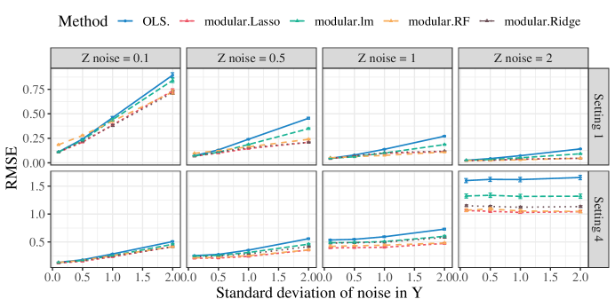
Figure 13: Aggregate RMSE in settings 1 and 4. Details are otherwise the same as Figure 3.

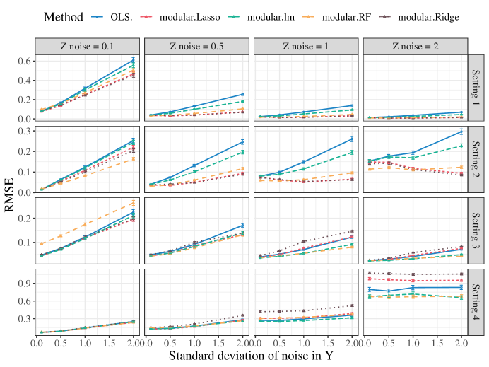
Figure 17: RMSE for estimating $\theta^{*}_{1}$ in all settings. Details are the same as Figure 3.

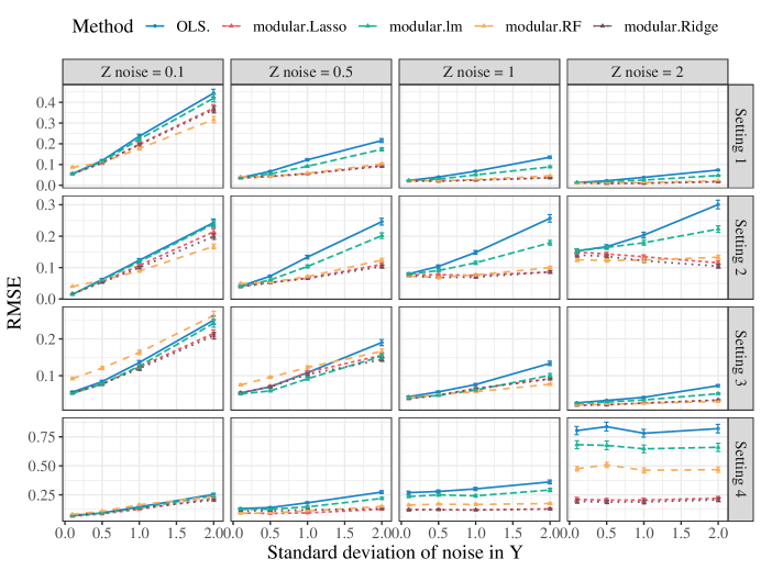
Figure 18: RMSE for estimating $\theta^{*}_{2}$ in all settings. Details are the same as Figure 3.

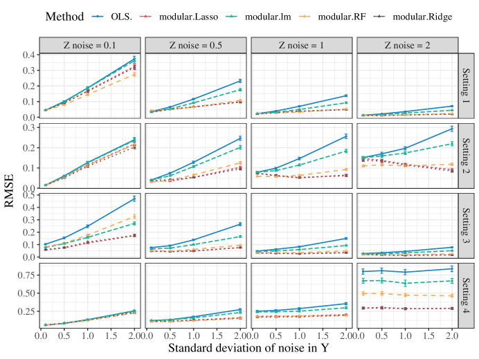
Figure 19: RMSE for estimating $\theta^{*}_{3}$ in all settings. Details are the same as Figure 3.

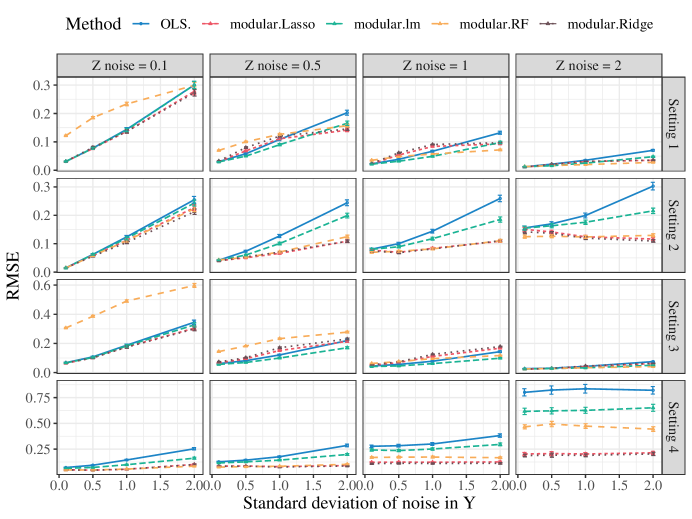
Figure 20: RMSE for estimating $\theta^{*}_{4}$ in all settings. Details are the same as Figure 3.

E.2 High-dimensional simulation

References

- Adragni and Cook, (2009) Adragni, K. P. and Cook, R. D. (2009). Sufficient dimension reduction and prediction in regression. Philosophical Transactions of the Royal Society A: Mathematical, Physical and Engineering Sciences, 367(1906):4385–4405.
- Athey et al., (2016) Athey, S., Chetty, R., Imbens, G., and Kang, H. (2016). Estimating treatment effects using multiple surrogates: The role of the surrogate score and the surrogate index. arXiv preprint arXiv:1603.09326.
- Athey et al., (2019) Athey, S., Chetty, R., Imbens, G. W., and Kang, H. (2019). The surrogate index: Combining short-term proxies to estimate long-term treatment effects more rapidly and precisely. Technical report, National Bureau of Economic Research.
- Banerjee et al., (2006) Banerjee, O., Ghaoui, L. E., d’Aspremont, A., and Natsoulis, G. (2006). Convex optimization techniques for fitting sparse gaussian graphical models. In Proceedings of the 23rd International Conference on Machine Learning, pages 89–96.
- Begg and Leung, (2000) Begg, C. B. and Leung, D. H. (2000). On the use of surrogate end points in randomized trials. Journal of the Royal Statistical Society: Series A (Statistics in Society), 163(1):15–28.
- Bickel et al., (1993) Bickel, P. J., Klaassen, C. A., Bickel, P. J., Ritov, Y., Klaassen, J., Wellner, J. A., and Ritov, Y. (1993). Efficient and Adaptive Estimation for Semiparametric Models, volume 4. Springer.
- Bickel et al., (2009) Bickel, P. J., Ritov, Y., and Tsybakov, A. B. (2009). Simultaneous analysis of lasso and dantzig selector. The Annals of Statistics, 37(4):1705–1732.
- Bühlmann, (2010) Bühlmann, P. (2010). Proposing the vote of thanks: Regression shrinkage and selection via the lasso: a retrospective by robert tibshirani.
- Bühlmann and Van De Geer, (2011) Bühlmann, P. and Van De Geer, S. (2011). Statistics for high-dimensional data: methods, theory and applications. Springer Science & Business Media.
- Cai and Zhang, (2016) Cai, T. T. and Zhang, A. (2016). Minimax rate-optimal estimation of high-dimensional covariance matrices with incomplete data. Journal of Multivariate Analysis, 150:55–74.
- Candes and Tao, (2007) Candes, E. and Tao, T. (2007). The dantzig selector: Statistical estimation when p is much larger than n. The Annals of Statistics, 35(6):2313–2351.
- Candes and Tao, (2005) Candes, E. J. and Tao, T. (2005). Decoding by linear programming. IEEE Transactions on Information Theory, 51(12):4203–4215.
- Cannings and Fan, (2022) Cannings, T. I. and Fan, Y. (2022). The correlation-assisted missing data estimator. Journal of Machine Learning Research, 23:41–1.
- Causeur and Dhorne, (2003) Causeur, D. and Dhorne, T. (2003). Linear regression models under conditional independence restrictions. Scandinavian Journal of Statistics, 30(3):637–650.
- Chen et al., (2007) Chen, H., Geng, Z., and Jia, J. (2007). Criteria for surrogate end points. Journal of the Royal Statistical Society: Series B (Statistical Methodology), 69(5):919–932.
- Chen, (2007) Chen, X. (2007). Large sample sieve estimation of semi-nonparametric models. Handbook of econometrics, 6:5549–5632.
- Chen and Shen, (1998) Chen, X. and Shen, X. (1998). Sieve extremum estimates for weakly dependent data. Econometrica, pages 289–314.
- Chernozhukov et al., (2018) Chernozhukov, V., Chetverikov, D., Demirer, M., Duflo, E., Hansen, C., Newey, W., and Robins, J. (2018). Double/debiased machine learning for treatment and structural parameters. The Econometrics Journal, 21(1):C1–C68.
- Chernozhukov et al., (2017) Chernozhukov, V., Hansen, C., and Liao, Y. (2017). A lava attack on the recovery of sums of dense and sparse signals. The Annals of Statistics, 45(1):39–76.
- Colnet et al., (2020) Colnet, B., Mayer, I., Chen, G., Dieng, A., Li, R., Varoquaux, G., Vert, J.-P., Josse, J., and Yang, S. (2020). Causal inference methods for combining randomized trials and observational studies: a review. arXiv preprint arXiv:2011.08047.
- Dahabreh et al., (2019) Dahabreh, I. J., Robertson, S. E., Tchetgen, E. J., Stuart, E. A., and Hernán, M. A. (2019). Generalizing causal inferences from individuals in randomized trials to all trial-eligible individuals. Biometrics, 75(2):685–694.
- Elsener and van de Geer, (2019) Elsener, A. and van de Geer, S. (2019). Sparse spectral estimation with missing and corrupted measurements. Stat, 8(1):e229.
- Fleming et al., (1994) Fleming, T. R., Prentice, R. L., Pepe, M. S., and Glidden, D. (1994). Surrogate and auxiliary endpoints in clinical trials, with potential applications in cancer and aids research. Statistics in Medicine, 13(9):955–968.
- Friedman et al., (2010) Friedman, J., Hastie, T., and Tibshirani, R. (2010). Regularization paths for generalized linear models via coordinate descent. Journal of Statistical Software, 33(1):1–22.
- Friedman et al., (1999) Friedman, N., Nachman, I., and Peér, D. (1999). Learning bayesian network structure from massive datasets: The ”sparse candidate” algorithm. In Proceedings of the Fifteenth Conference on Uncertainty in Artificial Intelligence, UAI’99, page 206–215, San Francisco, CA, USA. Morgan Kaufmann Publishers Inc.
- Hansen, (1982) Hansen, L. P. (1982). Large sample properties of generalized method of moments estimators. Econometrica: Journal of the Econometric Society, pages 1029–1054.
- Hartman et al., (2015) Hartman, E., Grieve, R., Ramsahai, R., and Sekhon, J. S. (2015). From sample average treatment effect to population average treatment effect on the treated: combining experimental with observational studies to estimate population treatment effects. Journal of the Royal Statistical Society: Series A (Statistics in Society), 178(3):757–778.
- Hastie et al., (2009) Hastie, T., Tibshirani, R., Friedman, J. H., and Friedman, J. H. (2009). The elements of statistical learning: data mining, inference, and prediction, volume 2. Springer.
- Henckel et al., (2019) Henckel, L., Perković, E., and Maathuis, M. H. (2019). Graphical criteria for efficient total effect estimation via adjustment in causal linear models. arXiv preprint arXiv:1907.02435.
- Javanmard and Montanari, (2014) Javanmard, A. and Montanari, A. (2014). Confidence intervals and hypothesis testing for high-dimensional regression. The Journal of Machine Learning Research, 15(1):2869–2909.
- Jin and Rothenhäusler, (2021) Jin, Y. and Rothenhäusler, D. (2021). Attribute-adaptive statistical inference for finite populations under distribution shift. arXiv preprint arXiv:2104.04565.
- Jordan, (1999) Jordan, M. I. (1999). Learning in graphical models. MIT Press.
- Kallus and Mao, (2020) Kallus, N. and Mao, X. (2020). On the role of surrogates in the efficient estimation of treatment effects with limited outcome data. arXiv preprint arXiv:2003.12408.
- Lam and Bacchus, (1994) Lam, W. and Bacchus, F. (1994). Learning bayesian belief networks: An approach based on the mdl principle. Computational Intelligence, 10(3):269–293.
- Lauritzen et al., (2004) Lauritzen, S. L., Aalen, O. O., Rubin, D. B., and Arjas, E. (2004). Discussion on causality [with reply]. Scandinavian Journal of Statistics, 31(2):189–201.
- Lee et al., (2006) Lee, S.-I., Ganapathi, V., and Koller, D. (2006). Efficient structure learning of markov networks using -regularization. Advances in Neural Information Processing Systems, 19.
- Li, (2018) Li, B. (2018). Sufficient dimension reduction: Methods and applications with R. Chapman and Hall/CRC.
- Li, (1991) Li, K.-C. (1991). Sliced inverse regression for dimension reduction. Journal of the American Statistical Association, 86(414):316–327.
- Loh and Wainwright, (2011) Loh, P.-L. and Wainwright, M. J. (2011). High-dimensional regression with noisy and missing data: Provable guarantees with non-convexity. Advances in Neural Information Processing Systems, 24.
- Lounici, (2014) Lounici, K. (2014). High-dimensional covariance matrix estimation with missing observations. Bernoulli, 20(3):1029–1058.
- Ma and Zhu, (2013) Ma, Y. and Zhu, L. (2013). Efficient estimation in sufficient dimension reduction. The Annals of Statistics.
- Margaritis and Thrun, (1999) Margaritis, D. and Thrun, S. (1999). Bayesian network induction via local neighborhoods. Advances in Neural Information Processing Systems, 12.
- Meinshausen and Bühlmann, (2006) Meinshausen, N. and Bühlmann, P. (2006). High-dimensional graphs and variable selection with the lasso. The Annals of Statistics, 34(3):1436–1462.
- Negahban et al., (2012) Negahban, S. N., Ravikumar, P., Wainwright, M. J., and Yu, B. (2012). A unified framework for high-dimensional analysis of -estimators with decomposable regularizers. Statistical Science, 27(4):538–557.
- Oldfield et al., (2021) Oldfield, Z., Rogers, N., Phelps, A., Blake, M., Steptoe, A., Oskala, A., Marmot, M., Clemens, S., Nazroo, J., and Banks, J. (2021). English longitudinal study of ageing: Waves 0-9, 1998-2019.
- Post et al., (2010) Post, W. J., Buijs, C., Stolk, R. P., de Vries, E. G., and Le Cessie, S. (2010). The analysis of longitudinal quality of life measures with informative drop-out: a pattern mixture approach. Quality of Life Research, 19(1):137–148.
- Prentice, (1989) Prentice, R. L. (1989). Surrogate endpoints in clinical trials: definition and operational criteria. Statistics in Medicine, 8(4):431–440.
- Robins et al., (2008) Robins, J., Li, L., Tchetgen, E., van der Vaart, A., et al. (2008). Higher order influence functions and minimax estimation of nonlinear functionals. In Probability and statistics: essays in honor of David A. Freedman, volume 2, pages 335–422. Institute of Mathematical Statistics.
- Robins et al., (1994) Robins, J. M., Rotnitzky, A., and Zhao, L. P. (1994). Estimation of regression coefficients when some regressors are not always observed. Journal of the American statistical Association, 89(427):846–866.
- Rosenman et al., (2020) Rosenman, E., Basse, G., Owen, A., and Baiocchi, M. (2020). Combining observational and experimental datasets using shrinkage estimators. arXiv preprint arXiv:2002.06708.
- Rosenman et al., (2022) Rosenman, E. T., Owen, A. B., Baiocchi, M., and Banack, H. R. (2022). Propensity score methods for merging observational and experimental datasets. Statistics in Medicine, 41(1):65–86.
- Roth, (2004) Roth, V. (2004). The generalized lasso. IEEE Transactions on Neural Networks, 15(1):16–28.
- Rotnitzky and Smucler, (2019) Rotnitzky, A. and Smucler, E. (2019). Efficient adjustment sets for population average treatment effect estimation in non-parametric causal graphical models. arXiv preprint arXiv:1912.00306.
- Rotnitzky et al., (2021) Rotnitzky, A., Smucler, E., and Robins, J. M. (2021). Characterization of parameters with a mixed bias property. Biometrika, 108(1):231–238.
- Sargan, (1958) Sargan, J. D. (1958). The estimation of economic relationships using instrumental variables. Econometrica: Journal of the Econometric Society, pages 393–415.
- Spirtes et al., (2000) Spirtes, P., Glymour, C. N., Scheines, R., and Heckerman, D. (2000). Causation, prediction, and search. MIT press.
- Tibshirani, (1996) Tibshirani, R. (1996). Regression shrinkage and selection via the lasso. Journal of the Royal Statistical Society: Series B (Methodological), 58(1):267–288.
- Tsamardinos et al., (2006) Tsamardinos, I., Brown, L. E., and Aliferis, C. F. (2006). The max-min hill-climbing bayesian network structure learning algorithm. Machine Learning, 65(1):31–78.
- Tsiatis, (2006) Tsiatis, A. A. (2006). Semiparametric theory and missing data. Springer.
- Van de Geer, (2007) Van de Geer, S. (2007). The deterministic lasso. ETH Zürich research collection.
- Van de Geer et al., (2014) Van de Geer, S., Bühlmann, P., Ritov, Y., and Dezeure, R. (2014). On asymptotically optimal confidence regions and tests for high-dimensional models. The Annals of Statistics.
- Van De Geer and Bühlmann, (2009) Van De Geer, S. A. and Bühlmann, P. (2009). On the conditions used to prove oracle results for the lasso.
- Van der Laan and Robins, (2003) Van der Laan, M. J. and Robins, J. M. (2003). Unified methods for censored longitudinal data and causality, volume 5. Springer.
- Van der Vaart, (2000) Van der Vaart, A. W. (2000). Asymptotic Statistics, volume 3. Cambridge University Press.
- VanderWeele, (2013) VanderWeele, T. J. (2013). Surrogate measures and consistent surrogates. Biometrics, 69(3):561–565.
- Vershynin, (2018) Vershynin, R. (2018). High-dimensional probability: An introduction with applications in data science, volume 47. Cambridge University Press.
- Zhang and Huang, (2008) Zhang, C.-H. and Huang, J. (2008). The sparsity and bias of the lasso selection in high-dimensional linear regression. The Annals of Statistics, 36(4):1567–1594.
- Zhang and Zhang, (2014) Zhang, C.-H. and Zhang, S. S. (2014). Confidence intervals for low dimensional parameters in high dimensional linear models. Journal of the Royal Statistical Society: Series B: Statistical Methodology, pages 217–242.
- Zhao and Yu, (2006) Zhao, P. and Yu, B. (2006). On model selection consistency of lasso. The Journal of Machine Learning Research, 7:2541–2563.
- Zhu et al., (2019) Zhu, Z., Wang, T., and Samworth, R. J. (2019). High-dimensional principal component analysis with heterogeneous missingness. arXiv preprint arXiv:1906.12125.