Emergence of a stochastic resonance in machine learning

Abstract

Can noise be beneficial to machine-learning prediction of chaotic systems? Utilizing reservoir computers as a paradigm, we find that injecting noise to the training data can induce a stochastic resonance with significant benefits to both short-term prediction of the state variables and long-term prediction of the attractor of the system. A key to inducing the stochastic resonance is to include the amplitude of the noise in the set of hyperparameters for optimization. By so doing, the prediction accuracy, stability and horizon can be dramatically improved. The stochastic resonance phenomenon is demonstrated using two prototypical high-dimensional chaotic systems.

The interplay between noise and nonlinear dynamics often leads to surprising phenomena with potentially significant applications and thus has always been an active area of interdisciplinary research. It has been well documented that noise can be beneficial to applications of dynamical systems, e.g., enhancing the response of a nonlinear system to weak periodic signals, through mechanisms such as stochastic and coherence resonances [1, 2, 3, 4, 5, 6]. A parallel development in nonlinear dynamics is the important but challenging problem of model-free and data-based prediction of chaotic systems [7, 8, 9, 10, 11, 12, 13, 14, 15, 16, 17, 18, 19, 20, 21, 22, 23, 24, 25, 26, 27, 28, 29, 30]. In general, there are two kinds of forecasting problems: short term and long term. In short-term forecasting, the goal is to predict the detailed dynamical evolution of the state variables from specific initial conditions, typically for a few oscillation cycles (or Lyapunov times). In long term prediction, the aim is to generate the attractor of the system with the correct statistical behaviors. According to conventional wisdom, for solving the prediction problems, typically noise is detrimental. For example, in short-term prediction, because of the sensitive dependence on initial conditions, noise will make the predicted state evolution diverge exponentially from the true one. In long-term prediction, noise can induce the trajectory to cross the basin boundary, leading to a wrong attractor.

In this paper, we report the counterintuitive phenomenon that, in model-free prediction of chaotic systems with machine learning, a certain amount of noise can significantly enhance the prediction accuracy and robustness. Similar to a stochastic resonance, too little or too much noise is not useful and may even downgrade the predictive power of the neural machine, but an optimal amount of noise can be beneficial. A central issue is then to determine the optimal noise level, which we solve using a generalized scheme of hyperparameter optimization. To be concrete, we focus on reservoir computing [31, 32, 33, 34] that has become a paradigm in machine-learning based prediction of nonlinear dynamical systems [35, 36, 37, 38, 39, 40, 41, 42, 43, 44, 45, 46, 47, 48, 49, 50, 51, 52] and inject noise into the input signal. A reservoir computer contains a number of hyperparameters and the prediction performance depends strongly on their values. Our simulations have revealed that, if the hyperparameters are not optimized, noise in the training data can improve to certain extent the prediction performance. However, in order to maximize the predictive power of a reservoir computer, it is necessary to find the optimal values of the hyperparameters, a task that can be accomplished through, e.g., Bayesian optimization [53, 54]. The key to the emergence of a stochastic resonance is to treat the noise amplitude as one of the hyperparameters, i.e., to regard it as an intrinsic parameter of the reservoir computer. Bayesian optimization can then yield the optimal noise level. We demonstrate using two prototypical high-dimensional chaotic systems that noise with the so-determined amplitude can generate more accurate, robust and stable predictions in both short and long terms through a stochastic resonance.

The basic principle of reservoir computing and the optimization method are described in Supplementary Information (SI) [55]. There are six hyperparameters to be optimized: the spectral radius $\rho$ of the reservoir network, the scaling factor $\gamma$ of the input weights, the leakage parameter $\alpha$, the regularization coefficient $\beta$, the link connection probability $p$ of the random network in the hidden layer, and the noise amplitude $\sigma$. To determine the optimal hyperparameter values, we use the surrogateopt function in Matlab [56], a Bayesian optimization procedure, and employ a surrogate approximation function to estimate the objective function and to find the global minimum through sampling and updating. Specifically, the surrogateopt algorithm [57] first samples several random points and evaluates the objective function at these trial points. The algorithm then creates a surrogate model of the objective function by interpolating a radial basis function through all the random trial points. From the surrogate function, the algorithm identifies the potential minima and samples the points about these minima to update the function.

We demonstrate the benefits of noise to both short-term and long-term prediction using two prototypical chaotic systems: the Mackey-Glass (MG) system described by a nonlinear delay differential equation and the spatiotemporal chaotic Kuramoto-Sivashinsky (KS) system. We use the Bayesian algorithm to obtain the optimal values of the six hyperparameters (including the noise amplitude $\sigma$). We then choose a number of $\sigma$ values away from the optimal value and test the prediction performance. For each such fixed $\sigma$ value, we optimize the other five hyperparameters. For a different value of $\sigma$, the set of the other five hyperparameters is then different. As we will demonstrate, as the noise amplitude deviates from the optimal value on either side, there is a gradual deterioration of the prediction performance, signifying the emergence of a stochastic resonance.

Our first example is the MG system [58] described by $\dot{s}(t)=as(t-\tau)/\left(1+\left[s(t-\tau)\right]^{c}\right)-bs(t)$, where $\tau$ is the time delay, $a$, $b$ and $c$ are parameters. The state of the system at time $t$ is determined by the entire prior state history within the time delay, making the phase space of the system infinitely dimensional. To be concrete, we use two values of the time delay: $\tau=17$ and $\tau=30$, and fix the other three parameters as $a=0.2$, $b=0.1$, and $c=10$. For $\tau=17$, the system exhibits a chaotic attractor with one positive Lyapunov exponent: $\lambda_{+}\approx 0.006$. For $\tau=30$, the system has a chaotic attractor with two positive Lyapunov exponents [59]: $\lambda_{+}\approx 0.011$ and 0.003. To generate the one-dimensional MG time series data, we integrate the delay differential equation with the time step $h=0.01$ and generate the training and testing data by sampling the time series every 100 steps: $\Delta t=100h=1.0$, where $\Delta t$ is evolutionary time step of the dynamical network in the hidden layer of the reservoir computer. To remove any transient behavior, we disregard the first $10,000\Delta t$ in the training dataset. The length of training data is $T=150,000\Delta t$. The step after the training data marks the start of the testing data, whose length depends on whether the task is to make short-term or long-term prediction. The time series data are pre-processed by using $z$-score normalization: $z(t)=\left[s(t)-\bar{s}\right]/\sigma_{s}$, where $s(t)$ is the original time series, $\bar{s}$ and $\sigma_{s}$ are the mean and standard deviation of $s(t)$, respectively. For $\tau=17$ and $\tau=30$ in the MG system, the testing lengths for Bayesian optimization are $T_{\rm opt}=900\Delta t$ and $300\Delta t$, respectively, which are also the testing lengths for short-term prediction. The so obtained optimal hyperparameter values are listed in Tab. 1. Figure 1(a) shows, for $\tau=30$, representative results of short-term prediction of the state evolution, where Gaussian noise with the optimal amplitude is injected into the training time series. Results of long-term prediction in terms of the attractors in the plane $\{X\equiv s(t),Y\equiv s(t-\tau)\}$ are shown in Fig. 1(b). Visually and statistically, the predicted attractor cannot be distinguished from the true attractor. Prediction results for $\tau=17$ are presented in SI [55].

Figure 1: Short-term and long-term prediction of the MG system for $\tau=30$. The optimal noise amplitude is $10^{-1.97}$. (a) Machine predicted system evolution (red trace) in comparison with the ground truth (blue). The predicted state evolution agrees with the true evolution for a time period that contains about 15 local maxima ($T=500\Delta t$), a result that is significantly better than those without optimal noise. (b,c) Representation of the true and predicted attractor in the $\{X\equiv s(t),Y\equiv s(t-\tau)\}$ plane. The prediction time length is $T=10,000\Delta t$.

Table 1: Optimal hyperparameter values for MG and KS

System	$\rho$	$\gamma$	$\alpha$	$\beta$	$p$	$\sigma$
MG ($\tau=17$)	1.62	0.55	0.64	$10^{-6.0}$	0.99	$10^{-3.42}$
MG ($\tau=30$)	1.27	0.23	0.57	$10^{-6.4}$	0.09	$10^{-1.97}$
KS	0.01	0.35	0.62	$10^{-9.0}$	0.21	$10^{-2.35}$

Our second example is the one-dimensional KS system [60, 61], a paradigm not only in physics and chemistry but also in applications of reservoir computing for demonstrating the predictive power for high-dimensional dynamical systems [39]. The system equation is $\frac{\partial u}{\partial t}+\mu\frac{\partial^{4}u}{\partial x^{4}}+\phi(\frac{\partial^{2}u}{\partial x^{2}}+u\frac{\partial u}{\partial x})=0$, where $u(x,t)$ is a scalar field defined in the spatial domain $0\leq x\leq L$, $\mu$ and $\phi$ are parameters. We set $\mu=1$ and $\phi=1$, and use the periodic boundary condition. As the domain size $L$ increases, the system becomes progressively more high-dimensionally chaotic with the number of Lyapunov exponents increasing linearly with the system size [62]. As a representative case of high-dimensional chaos, we choose $L=60$, where the system has seven positive Lyapunov exponents: $\lambda_{+}\approx 0.089$, 0.067, 0.055, 0.041, 0.030, 0.005, and 0.003. The length of the training data is about 1000 Lyapunov times (after disregarding a transient of about 300 Lyapunov times), where a Lyapunov time is defined as the inverse of the largest positive exponent. The testing data for short-term and long-term prediction are taken immediately after the training data of six and 100 Lyapunov times, respectively.

Figure 2: Short-term and long-term prediction of the KS system. (a,b) True short-term (six Lyapunov times) and long-term (100 Lyapunov times) spatiotemporal evolution of the nonlinear field $u(x,t)$, respectively, (c,d) the predicted field $\hat{u}(x,t)$ in short and long terms, respectively. (e) Difference between the predicted and true fields defined as $D(x,t)\equiv\sqrt{\left[u(x,t)-\hat{u}(x,t)\right]^{2}}$. (f) Overlapped image of the true and predicted attractors in terms of the 4th and 5th dimension of the KS system. The values of the optimal hyperparameters (including the optimal noise amplitude) are listed in Tab. 1.

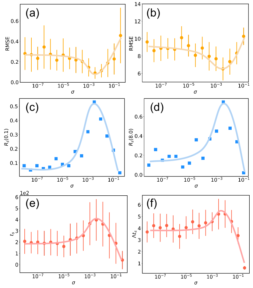
Figure 3: Stochastic resonance associated with short-term prediction of chaotic systems. Shown are three measures of short-term prediction versus the noise amplitude for two examples: left column - MG system for $\tau=30$ ($r_{c}=0.1$, length of prediction time window $=300\Delta t$), right column - KS system ($r_{c}=8.0$, length of prediction time window $=$ five Lyapunov times); top row - RMSE, middle row - prediction stability $R_{s}(r_{c})$, bottom row - prediction horizon $t_{s}$. The error bars are obtained from an ensemble of 80 performing reservoir computers. For each chaotic system, a specific and unique noise level emerges at which each prediction measure is optimized, which is characteristic of a stochastic resonance.

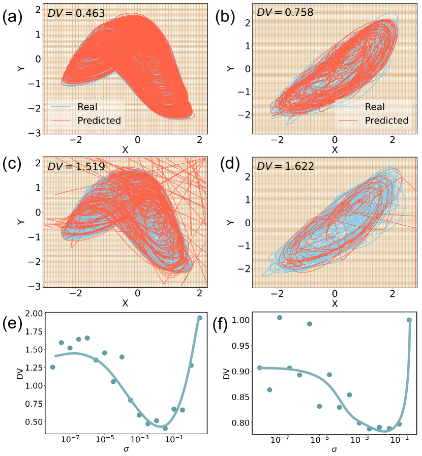
Figure 4: Quantifying long-term prediction through the deviation value DV. (a,b) Successful cases of attractor prediction in the presence of optimal noise for the MG system for $\tau=30$ and KS system, respectively. (c,d) Unsuccessful cases of attractor prediction without noise for the two systems. The two-dimensional phase space for the MG system is $\{X(t)\equiv s(t),Y(t)\equiv s(t-\tau)\}$. For the KS system, the space is $\{X(t)\equiv u(4,t),Y(t)\equiv u(5,t)\}$. (e,f) DV versus the noise amplitude for the MG and KS systems, respectively. There exists an optimal noise amplitude at which the DV value is minimized, which agrees with the optimal noise level determined from the corresponding short-term prediction results in Fig. 3.

Figure 2 shows the results of short-term and long-term predictions of the KS system. It can be seen that the reservoir computing machine with the aid of optimal noise not only can accurately predict the short-term spatiotemporal evolution but also is able to replicate the long-term attractor with the correct statistical behavior.

Associated with a conventional stochastic resonance in nonlinear systems, some performance measure such as the signal-to-noise ratio is maximized for an optimal noise level. Can a similar phenomenon arise in machine-learning prediction of chaotic systems, where the prediction performance reaches a maximum for an optimal noise level and deteriorates as the noise amplitude deviates from the optimal value? That is, how do we ascertain if the optimal noise amplitude values from Bayesian optimization as listed in Tab. 1 are indeed optimal?

To address these questions, we test the performance when the noise amplitude deviates from the optimal value. For any such fixed noise amplitude, the five other hyperparameters are optimized before training. In particular, we vary the noise amplitude (uniformly on a logarithmic scale) in the range $[10^{-8},10^{-0.5}]$. For each noise amplitude, we fix it during the Bayesian optimization and optimize the other five hyperparameters ($\rho$, $\gamma$, $\alpha$, $\beta$, and $k$). For different values of the noise amplitude, the so obtained values of the other five hyperparameters are listed in three Supplementary tables [55].

We demonstrate the emergence of a stochastic resonance for both short-term and long-term predictions. To characterize the performance of short-term prediction, besides the conventional RMSE (defined in SI [55]), we introduce two additional measures: prediction horizon and stability, where the former (denoted as $t_{s}$) is the maximal time interval during which the RMSE is below a threshold and the latter is the probability that a reservoir computer generates stable dynamical evolution of the target chaotic system in a fixed time window, which is defined as $R_{s}(r_{c})=(1/n)\sum_{i=1}^{n}\left[{\rm RMSE}<r_{c}\right]$, where $r_{c}$ is the RMSE threshold, $n$ is the number of iterations, and $\left[\cdot\right]=1$ if the statement inside is true and zero otherwise.

Figure 3 shows the RMSE, the prediction stability $R_{s}(r_{c})$, and the prediction horizon versus the noise amplitude $\sigma$ for the MG system for $\tau=30$ (left column, $r_{c}=0.1$), as well as the KS system (right column, $r_{c}=8.0$). In both cases, an optimal noise level emerges in the sense that a prediction measure versus the noise amplitude exhibits either a “bell shape” or an “anti-bell shape” type of variation about an optimal point. Figure 3 thus provides strong evidence for a stochastic resonance associated with short-term performance of machine-learning prediction of chaotic systems. The results for MG for $\tau=17$ are presented in SI [55].

We now demonstrate the emergence of a stochastic resonance from long-term prediction through a quantitative measure that we introduce to characterize the corresponding performance, as shown in Fig. 4 for the MG system for $\tau=30$ (left column) and the KS system (right column). The measure is the deviation value (DV), which characterizes the ability for a trained reservoir computer to capture the dynamical “climate” of the target system (its detailed definition can be found in SI [55]). In each case, there is an optimal noise amplitude at which the DV value is minimized [Figs. 4(e) and 4(f)], which agrees with the optimal value of the noise amplitude from the short-term prediction results in Fig. 3, providing additional support for the emergence of a stochastic resonance in machine learning in terms of long-term prediction of chaotic attractors. The emergence of such a stochastic resonance from long-term prediction for the MG system for $\tau=17$ is treated in SI [55].

To summarize, we have uncovered the emergence of a stochastic resonance in machine-learning prediction of chaotic systems. Focusing on reservoir computing, we find that injecting noise into the training data can be beneficial to both short- and long-term predictions. In particular, for short-term prediction, a number of characterizing quantities such as the prediction accuracy, stability, and horizon can be maximized by an optimal level of noise that can be found through hyperparameter optimization. For long-term prediction, optimal noise can significantly increase the chance for the machine generated trajectory to stay in the vicinity of (or to shadow) the true attractor of the target chaotic system. Intuitively, training with noise can enhance the machine’s tolerance to random fluctuations, which can be beneficial especially when the target system is chaotic. This argument suggests that the optimal noise level should be on the same order of magnitude as the one-step prediction error in noiseless prediction, which is indeed so as verified by our numerical examples. Our work extends the ubiquitous phenomenon of stochastic resonance in nonlinear dynamical systems to the realm of machine learning, where deliberate noise combined with hyperparameter optimization can be a practically feasible approach to enhancing the predictive power of the neural machine.

We note that, previously the role of noise in neural network training was studied, e.g., adding noise to the training data for convolutional neural networks can play the role of regularization to reduce overfitting in the learning models [63]. In reinforcement learning, injecting noise into the signals can help the system reach the persistent excitation condition to facilitate parameter estimation [64, 65]. How noise negatively affects the prediction of chaotic systems has recently been considered [66], where long short-term memory machines tend to be more resistant to noise than other machine-learning methods. The beneficial role of noise in machine-learning prediction has also been recognized [67, 68, 69, 70]. In spite of the previous efforts, to our knowledge, the interplay between noise and machine-learning prediction of dynamical systems was not systematically studied prior to our work. The discovery of stochastic resonance in machine learning fills this gap.

Finally, we remark that, in the vast literature on stochastic resonance, the paradigmatic model of mechanical motion of a particle in a double-well potential subject to stochastic forcing is often used to explain the observed resonance phenomenon. However, it is difficult to apply this model to our machine-learning system, as the dynamics of the high-dimensional neural network in the hidden layer of a reservoir computer are extraordinarily complicated. Nonetheless, the predictive ability of the reservoir computer can be related to generalized synchronization (see Sec. IV in SI [55]). Previous works in the past two decades demonstrated that noise can induce and enhance synchronization in nonlinear and complex dynamical systems [71, 72, 73, 74, 75, 76, 77, 78, 79, 80, 81]. We speculate that the mechanism responsible for the stochastic resonance phenomenon reported here is noise-enhance generalized synchronization.

This work was supported by AFOSR under Grant No. FA9550-21-1-0438.

References

- Benzi et al. [1981] R. Benzi, A. Sutera, and A. Vulpiani, The mechanism of stochastic resonance, J. Phys. A 14, L453 (1981).
- Benzi et al. [1983] R. Benzi, G. Parisi, A. Sutera, and A. Vulpiani, A theory of stochastic resonance in climatic-change, J. Appl. Math. 43, 565 (1983).
- McNamara and Wiesenfeld [1989] B. McNamara and K. Wiesenfeld, Theory of stochastic resonance, Phys. Rev. A 39, 4854 (1989).
- Moss et al. [1994] F. Moss, D. Pierson, and D. O’Gorman, Stochastic resonance - tutorial and update, Int. J. Bif. Chaos 4, 1383 (1994).
- Gailey et al. [1997] P. C. Gailey, A. Neiman, J. J. Collins, and F. Moss, Stochastic resonance in ensembles of nondynamical elements: The role of internal noise, Phys. Rev. Lett. 79, 4701 (1997).
- Gammaitoni et al. [1998] L. Gammaitoni, P. Hänggi, P. Jung, and F. Marchesoni, Stochastic resonance, Rev. Mod. Phys. 70, 223 (1998).
- Farmer and Sidorowich [1987] J. D. Farmer and J. J. Sidorowich, Predicting chaotic time series, Phys. Rev. Lett. 59, 845 (1987).
- Casdagli [1989] M. Casdagli, Nonlinear prediction of chaotic time series, Physica D 35, 335 (1989).
- Sugihara et al. [1990] G. Sugihara, B. Grenfell, R. M. May, P. Chesson, H. M. Platt, and M. Williamson, Distinguishing error from chaos in ecological time series, Phil. Trans. Roy. Soc. London B 330, 235 (1990).
- Kurths and Ruzmaikin [1990] J. Kurths and A. A. Ruzmaikin, On forecasting the sunspot numbers, Solar Phys. 126, 407 (1990).
- Grassberger and Schreiber [1990] P. Grassberger and T. Schreiber, Nonlinear time sequence analysis, Int. J. Bif. Chaos 1, 521 (1990).
- Gouesbet [1991] G. Gouesbet, Reconstruction of standard and inverse vector fields equivalent to a Rössler system, Phys. Rev. A 44, 6264 (1991).
- Tsonis and Elsner [1992] A. A. Tsonis and J. B. Elsner, Nonlinear prediction as a way of distinguishing chaos from random fractal sequences, Nature (London) 358, 217 (1992).
- Baake et al. [1992] E. Baake, M. Baake, H. G. Bock, and K. M. Briggs, Fitting ordinary differential equations to chaotic data, Phys. Rev. A 45, 5524 (1992).
- Crutchfield and McNamara [1987] J. P. Crutchfield and B. McNamara, Equations of motion from a data series, Complex Sys. 1, 417 (1987).
- Sauer [1994] T. Sauer, Reconstruction of dynamical systems from interspike intervals, Phys. Rev. Lett. 72, 3811 (1994).
- Sugihara [1994] G. Sugihara, Nonlinear forecasting for the classification of natural time series, Philos. T. Roy. Soc. A. 348, 477 (1994).
- Parlitz [1996] U. Parlitz, Estimating model parameters from time series by autosynchronization, Phys. Rev. Lett. 76, 1232 (1996).
- Schiff et al. [1996] S. J. Schiff, P. So, T. Chang, R. E. Burke, and T. Sauer, Detecting dynamical interdependence and generalized synchrony through mutual prediction in a neural ensemble, Phys. Rev. E 54, 6708 (1996).
- Hegger et al. [1999] R. Hegger, H. Kantz, and T. Schreiber, Practical implementation of nonlinear time series methods: The TISEAN package, Chaos 9, 413 (1999).
- Bollt [2000] E. M. Bollt, Controlling chaos and the inverse frobenius-perron problem: global stabilization of arbitrary invariant measures, Int. J. Bif. Chaos 10, 1033 (2000).
- Hegger et al. [2000] R. Hegger, H. Kantz, L. Matassini, and T. Schreiber, Coping with nonstationarity by overembedding, Phys. Rev. Lett. 84, 4092 (2000).
- Sello [2001] S. Sello, Solar cycle forecasting: a nonlinear dynamics approach, Astron. Astrophys. 377, 312 (2001).
- Matsumoto et al. [2001] T. Matsumoto, Y. Nakajima, M. Saito, J. Sugi, and H. Hamagishi, Reconstructions and predictions of nonlinear dynamical systems: a hierarchical bayesian approach, IEEE Trans. Signal Proc. 49, 2138 (2001).
- Smith [2002] L. A. Smith, What might we learn from climate forecasts?, Proc. Nat. Acad. Sci. (USA) 19, 2487 (2002).
- Judd [2003] K. Judd, Nonlinear state estimation, indistinguishable states, and the extended kalman filter, Physica D 183, 273 (2003).
- Sauer [2004] T. D. Sauer, Reconstruction of shared nonlinear dynamics in a network, Phys. Rev. Lett. 93, 198701 (2004).
- Tao et al. [2007] C. Tao, Y. Zhang, and J. J. Jiang, Estimating system parameters from chaotic time series with synchronization optimized by a genetic algorithm, Phys. Rev. E 76, 016209 (2007).
- Wang et al. [2011] W.-X. Wang, R. Yang, Y.-C. Lai, V. Kovanis, and C. Grebogi, Predicting catastrophes in nonlinear dynamical systems by compressive sensing, Phys. Rev. Lett. 106, 154101 (2011).
- Wang et al. [2016] W.-X. Wang, Y.-C. Lai, and C. Grebogi, Data based identification and prediction of nonlinear and complex dynamical systems, Phys. Rep. 644, 1 (2016).
- Jaeger [2001] H. Jaeger, The “echo state” approach to analysing and training recurrent neural networks-with an erratum note, Bonn, Germany: German National Research Center for Information Technology GMD Technical Report 148, 13 (2001).
- Mass et al. [2002] W. Mass, T. Nachtschlaeger, and H. Markram, Real-time computing without stable states: A new framework for neural computation based on perturbations, Neur. Comp. 14, 2531 (2002).
- Jaeger and Haas [2004] H. Jaeger and H. Haas, Harnessing nonlinearity: Predicting chaotic systems and saving energy in wireless communication, Science 304, 78 (2004).
- Manjunath and Jaeger [2013] G. Manjunath and H. Jaeger, Echo state property linked to an input: Exploring a fundamental characteristic of recurrent neural networks, Neur. Comp. 25, 671 (2013).
- Haynes et al. [2015] N. D. Haynes, M. C. Soriano, D. P. Rosin, I. Fischer, and D. J. Gauthier, Reservoir computing with a single time-delay autonomous Boolean node, Phys. Rev. E 91, 020801 (2015).
- Larger et al. [2017] L. Larger, A. Baylón-Fuentes, R. Martinenghi, V. S. Udaltsov, Y. K. Chembo, and M. Jacquot, High-speed photonic reservoir computing using a time-delay-based architecture: Million words per second classification, Phys. Rev. X 7, 011015 (2017).
- Pathak et al. [2017] J. Pathak, Z. Lu, B. Hunt, M. Girvan, and E. Ott, Using machine learning to replicate chaotic attractors and calculate Lyapunov exponents from data, Chaos 27, 121102 (2017).
- Duriez et al. [2017] T. Duriez, S. L. Brunton, and B. R. Noack, Machine Learning Control-Taming Nonlinear Dynamics and Turbulence (Springer, 2017).
- Pathak et al. [2018] J. Pathak, B. Hunt, M. Girvan, Z. Lu, and E. Ott, Model-free prediction of large spatiotemporally chaotic systems from data: A reservoir computing approach, Phys. Rev. Lett. 120, 024102 (2018).
- Carroll [2018] T. L. Carroll, Using reservoir computers to distinguish chaotic signals, Phys. Rev. E 98, 052209 (2018).
- Roland and Parlitz [2018] Z. S. Roland and U. Parlitz, Observing spatio-temporal dynamics of excitable media using reservoir computing, Chaos 28, 043118 (2018).
- Griffith et al. [2019] A. Griffith, A. Pomerance, and D. J. Gauthier, Forecasting chaotic systems with very low connectivity reservoir computers, Chaos 29, 123108 (2019).
- Jiang and Lai [2019] J. Jiang and Y.-C. Lai, Model-free prediction of spatiotemporal dynamical systems with recurrent neural networks: Role of network spectral radius, Phys. Rev. Research 1, 033056 (2019).
- Fan et al. [2020] H. Fan, J. Jiang, C. Zhang, X. Wang, and Y.-C. Lai, Long-term prediction of chaotic systems with machine learning, Phys. Rev. Research 2, 012080 (2020).
- Klos et al. [2020] C. Klos, Y. F. K. Kossio, S. Goedeke, A. Gilra, and R.-M. Memmesheimer, Dynamical learning of dynamics, Phys. Rev. Lett. 125, 088103 (2020).
- Vlachasa et al. [2020] P. R. Vlachasa, P. J., B. R. Hunt, T. P. Sapsis, M. Girvan, E. Ott, and P. Koumoutsakos, Backpropagation algorithms and reservoir computing in recurrent neural networks for the forecasting of complex spatiotemporal dynamics, Neu. Net. 126, 191 (2020).
- Kong et al. [2021a] L.-W. Kong, H.-W. Fan, C. Grebogi, and Y.-C. Lai, Machine learning prediction of critical transition and system collapse, Phys. Rev. Research 3, 013090 (2021a).
- Kim et al. [2021] J. Z. Kim, Z. Lu, E. Nozari, G. J. Pappas, and D. S. Bassett, Teaching recurrent neural networks to infer global temporal structure from local examples, Nat. Machine Intell. 3, 316 (2021).
- Fan et al. [2021] H. Fan, L.-W. Kong, Y.-C. Lai, and X. Wang, Anticipating synchronization with machine learning, Phys. Rev. Resesearch 3, 023237 (2021).
- Kong et al. [2021b] L.-W. Kong, H.-W. Fan, C. Grebogi, and Y.-C. Lai, Emergence of transient chaos and intermittency in machine learning, J. Phys. Complex. 2, 035014 (2021b).
- Bollt [2021] E. Bollt, On explaining the surprising success of reservoir computing forecaster of chaos? the universal machine learning dynamical system with contrast to VAR and DMD, Chaos 31, 013108 (2021).
- Gauthier et al. [2021] D. J. Gauthier, E. Bollt, A. Griffith, and W. A. S. Barbosa, Next generation reservoir computing, Nat. Commun. 12, 5564 (2021).
- Snoek et al. [2012] J. Snoek, H. Larochelle, and R. P. Adams, Practical Bayesian optimization of machine learning algorithms, in Advances in Neural Information Processing Systems, Vol. 25, edited by F. Pereira, C. Burges, L. Bottou, and K. Weinberger (Curran Associates, Inc., 2012).
- Yang and Shami [2020] L. Yang and A. Shami, On hyperparameter optimization of machine learning algorithms: Theory and practice, Neurocomp. 415, 295 (2020).
- [55] Supplementary Information provides additional details of the results in the main text. It is helpful but not essential for understanding the main results of the paper. It contains the following materials: a brief description of the the principle of reservoir computing for predicting chaotic systems, the lists of optimized hyperparameter values used in demonstrating the emergence of a stochastic resonance for the numerical examples, and a number of pertinent issues such as the prediction time required for a stochastic resonance, its robustness against different scenarios of noise injection, and the benefits of noise to reducing the reservoir network size for predicting chaotic systems, as well as a plausible dynamical mechanism for the observed resonance phenomenon .
- sur [a] Surrogate optimization for global minimization of time-consuming objective functions - MATLAB, https://www.mathworks.com/help/gads/surrogateopt.html (a).
- sur [b] Surrogate optimization algorithm - MATLAB, https://www.mathworks.com/help/gads/surrogate-optimization-algorithm.html (b).
- Mackey and Glass [1977] M. C. Mackey and L. Glass, Oscillation and chaos in physiological control systems, Science 197, 287 (1977).
- Wernecke et al. [2019] H. Wernecke, B. Sándor, and C. Gros, Chaos in time delay systems: An educational review, Phys. Rep. 824, 1 (2019).
- Koramoto and Tsuzuki [1976] Y. Koramoto and T. Tsuzuki, Persistent propagation of concentration waves in dissipative media far from thermal equilibrium, Prof. Theor. Phys. 55, 356 (1976).
- Sivashinsky [1977] G. I. Sivashinsky, Nonlinear analysis of hydrodynamic instability in laminar ames I. derivation of basic equations, Acta Astron. 4, 1177 (1977).
- Edson et al. [2019] R. A. Edson, J. E. Bunder, T. W. Mattner, and A. J. Roberts, Lyapunov exponents of the Kuramoto–Sivashinsky PDE, ANZIAM J. 61, 270 (2019).
- Smilkov et al. [2017] D. Smilkov, N. Thorat, B. Kim, F. Viégas, and M. Wattenberg, Smoothgrad: removing noise by adding noise, arXiv preprint arXiv:1706.03825 (2017).
- Xu et al. [2013] B. Xu, C. Yang, and Z. Shi, Reinforcement learning output feedback NN control using deterministic learning technique, IEEE Trans. Neu. Net. Learning Sys. 25, 635 (2013).
- Kamalapurkar et al. [2016] R. Kamalapurkar, P. Walters, and W. E. Dixon, Model-based reinforcement learning for approximate optimal regulation, Automatica 64, 94 (2016).
- Sangiorgio et al. [2021] M. Sangiorgio, F. Dercole, and G. Guariso, Forecasting of noisy chaotic systems with deep neural networks, Chaos Soli. Frac. 153, 111570 (2021).
- Bishop [1995] C. M. Bishop, Training with noise is equivalent to tikhonov regularization, Neu. Comp. 7, 108 (1995).
- Grandvalet et al. [1997] Y. Grandvalet, S. Canu, and S. Boucheron, Noise injection: Theoretical prospects, Neural Computation 9, 1093 (1997).
- Wyffels et al. [2008] F. Wyffels, B. Schrauwen, and D. Stroobandt, Stable output feedback in reservoir computing using ridge regression, in International conference on artificial neural networks (Springer, 2008) pp. 808–817.
- Jim et al. [1996] K.-C. Jim, C. L. Giles, and B. G. Horne, An analysis of noise in recurrent neural networks: convergence and generalization, IEEE Trans. Neu. Net. 7, 1424 (1996).
- Toral et al. [2001] R. Toral, C. R. Mirasso, E. Hernandez-Garcia, and O. Piro, Analytical and numerical studies of noise induced synchronization of chaotic systems, Chaos 11, 665 (2001).
- He et al. [2003] D. He, P. Shi, and L. Stone, Noise-induced synchronization in realistic models, Phys. Rev. E 67, 027201 (2003).
- Guan et al. [2006] S. Guan, Y.-C. Lai, C.-H. Lai, and X. Gong, Understanding synchronization induced by common noise, Phys. Lett. A 353, 30 (2006).
- Wang et al. [2010] Y. Wang, Y.-C. Lai, and Z. Zheng, Route to noise-induced synchronization in an ensemble of uncoupled chaotic systems, Phys. Rev. E 81, 036201 (2010).
- Nakao et al. [2007] H. Nakao, K. Arai, and Y. Kawamura, Noise-induced synchronization and clustering in ensembles of uncoupled limit-cycle oscillators, Phys. Rev. Lett. 98, 184101 (2007).
- Esfahani et al. [2012] R. K. Esfahani, F. Shahbazi, and K. A. Samani, Noise-induced synchronization in small world networks of phase oscillators, Phys. Rev. E 86, 036204 (2012).
- Lai and Porter [2013] Y. M. Lai and M. A. Porter, Noise-induced synchronization, desynchronization, and clustering in globally coupled nonidentical oscillators, Phys. Rev. E 88, 012905 (2013).
- Kurebayashi et al. [2014] W. Kurebayashi, T. Ishii, M. Hasegawa, and H. Nakao, Design and control of noise-induced synchronization patterns, EPL 107, 10009 (2014).
- Russo and Shorten [2018] G. Russo and R. Shorten, On common noise-induced synchronization in complex networks with state-dependent noise diffusion processes, Physisca D 369, 47 (2018).
- Touboul et al. [2020] J. D. Touboul, C. Piette, L. Venance, and G. B. Ermentrout, Noise-induced synchronization and antiresonance in interacting excitable systems: Applications to deep brain stimulation in parkinson’s disease, Phys. Rev. X 10, 011073 (2020).
- Shajan et al. [2021] E. Shajan, M. P. Asir, S. Dixit, J. Kurths, and M. D. Shrimali, Enhanced synchronization due to intermittent noise, New J. Phys. 23, 112001 (2021).