VeriCompress: A Tool to Streamline the Synthesis of Verified Robust Compressed Neural Networks from Scratch

Abstract

AI’s widespread integration has led to neural networks (NNs) deployment on edge and similar limited-resource platforms for safety-critical scenarios. Yet, NN’s fragility raises concerns about reliable inference. Moreover, constrained platforms demand compact networks. This study introduces VeriCompress, a tool that automates the search and training of compressed models with robustness guarantees. These models are well-suited for safety-critical applications and adhere to predefined architecture and size limitations, making them deployable on resource-restricted platforms. The method trains models $2-3$ times faster than the state-of-the-art approaches, surpassing relevant baseline approaches by average accuracy and robustness gains of $15.1$ and $9.8$ percentage points, respectively. When deployed on a resource-restricted generic platform, these models require $5-8$ times less memory and $2-4$ times less inference time than models used in verified robustness literature. Our comprehensive evaluation across various model architectures and datasets, including MNIST, CIFAR, SVHN, and a relevant pedestrian detection dataset, showcases VeriCompress’s capacity to identify compressed verified robust models with reduced computation overhead compared to current standards. This underscores its potential as a valuable tool for end users, such as developers of safety-critical applications on edge or Internet of Things platforms, empowering them to create suitable models for safety-critical, resource-constrained platforms in their respective domains.

1 Introduction

Neural Networks (NNs) are vulnerable to small deviations in the input, i.e., imperceptible adversarial perturbation defined by the perturbation budget $\varepsilon$, which can lead to inaccurate inferences (Goodfellow, Shlens, and Szegedy 2015). Such vulnerability may have catastrophic effects (Pereira and Thomas 2020) in safety-critical real-world applications such as medical diagnosis or autonomous driving, where the input data may often be slightly changed due to sensor noise, measurement errors, or adversarial attacks.

Although Madry et al. (2018) introduced PGD adversarial training to boost robustness, Gowal et al. (2018) revealed that such training doesn’t guarantee robustness. Adversarial samples were discovered near the supposedly robust ones, raising concerns for safety-critical applications such as ACAS-Xu, pedestrian detection, and healthcare (Katz et al. 2017; Kim, Park, and Ro 2021; Guo et al. 2023).

To address this, Verified robustness training methods (Katz et al. 2017; Gowal et al. 2018; Zhang et al. 2020; Xu et al. 2020) were developed, providing robustness guarantees. These methods certify the absence of adversarial samples near robust ones. However, they achieve verified robustness at the expense of accuracy (Zhang et al. 2020; Xu et al. 2020). Despite this trade-off, ensuring robustness within specific feature space regions is crucial for the secure implementation of sensitive applications. E.g., these robustness assurances have been used to partition the feature space into regions of varying robustness for ACAS-Xu (Julian et al. 2019). This division facilitates training hierarchical models that exhibit high robustness in different feature space regions, thereby enhancing the reliability of neural network decisions in safety-critical contexts. Detailed background on verified robustness training is in Appendix A.

A challenge that yet remains unresolved is that many real-world safety-critical applications demand NNs to be deployed on resource-constraint platforms, such as drones, self-driving cars, smart-watches, etc., which kindles the need for highly compressed models, requiring significantly low computation and storage resources, all while achieving accuracy and verified robustness comparable to the denser counterparts developed in state-of-the-art. Finding such compressed verified robust NN architectures requires extensive computations, compounded by model size limitations. Moreover, the architecture varies based on applications, necessitating domain knowledge. E.g., image classification leans on convolutional layers (CNNs), while image captioning benefits from sequential architectures (RNNs).

This work aims to automate the exploration of compressed networks while concurrently training a verified robust model within the confines of a parameter-budget—an estimated count of parameters for the required compressed model suitable for resource-constrained device deployment. The paper presents VeriCompress, a tool enabling users to choose a desired architecture type in the form of an existing complex/dense randomly initialized model, defined as backbone architecture, and a parameter budget. VeriCompress then automatically identifies a compressed architecture, i.e., a sub-network within the specified backbone that meets the parameter budget while attaining similar accuracy and verified robustness compared to denser models.

Research Gap being Addressed: Amid various pruning techniques, structured model pruning stands out for effectively decreasing model size and computational resources (Sadou et al. 2022) (refer to Appendix B for details). However, the leading pruning methods, Hydra (Sehwag et al. 2020) and Fashapley (Kang, Li, and Li 2023), designed to ensure verified robustness, exhibit suboptimal performance when applied to structured pruning. Additionally, these techniques necessitate prior training of the original dense model, leading to substantial resource and time burdens. In contrast, VeriCompress streamlines the process by initiating from a randomly initialized large model (backbone), considerably reducing training time and resource overhead. Moreover, VeriCompress simultaneously achieves relatively higher generalizability compared to state-of-the-art robust pruning approaches (Sehwag et al. 2020; Kang, Li, and Li 2023). In this work, we refer to model generalizability as the ability of the model to project high-standard accuracy and verified robustness simultaneously.

The paper’s contributions are summarized below:

1. This is the first work to demonstrate that verified robust compressed neural networks can be trained from scratch while outperforming baseline works (Sehwag et al. 2020; Kang, Li, and Li 2023) by an average of $15.1$ and $9.8$ percent points in accuracy and verified robustness.

2. VeriCompress extracts compressed NNs taking $2-3$ times less training time than state-of-the-art structured pruning approaches in the same platform.

3. The compressed models thus achieved, when deployed on a resource-constrained generic platform, such as Google Pixel 6, require about $5-8$ times less memory and $2-4$ times less inference time compared to the starting architecture.

4. Our empirical study demonstrates that VeriCompress performs effectively on benchmark datasets (CIFAR-10, MNIST, & SVHN) and application-relevant Pedestrian Detection (N J Karthika 2020) dataset, and model architecture combinations used in the literature.

The following sections provide related work discussion, details of the approach, and supporting evaluations. Additionally, Appendices include relevant background.

2 Related work

With the recent advances in verified robustness, to the best of our knowledge, two recent works have aimed at achieving compressed networks that exhibit verified robutness (Sehwag et al. 2020; Kang, Li, and Li 2023).

Sehwag et al. (2020) (Hydra) proposed a three-step robustness-aware model training approach accounting for both adversarial robustness and verified robustness (also known as certified robustness). The pre-train step aims to generate a robust dense model, which then undergoes prune-training to learn a robustness-aware importance score for each parameter, which guides the final pruning mask. The finetuning step updates the retained weights to recover the model’s performance. Hydra sets an equal pruning ratio for all the layers to obtain the pruning mask, which ignores the fact that different layers hold different importance toward model inference.

Kang, Li, and Li (2023) developed FaShapley following Hydra’s framework with the difference in the prune-training step. The update to a parameter’s importance scores is equivalent to the magnitude of the product of weight and gradient, which is an efficient approximation for its shapely value. The final removal of weights can be done in a structured or unstructured manner based on the importance scores (Shapley values) considered globally.

This paper considers Hydra (Sehwag et al. 2020) and Fashapley (Kang, Li, and Li 2023) as baselines and shows their performance comparisons with VeriCompress.

3 Parameter-Budget-Aware Architecture Search for Verified Robust Models

VeriCompress is a tool that takes an initially over-parameterized randomly initialized NN architecture, serving as the backbone (essentially representing the desired architecture type), along with a parameter budget, and it then searches and identifies a verified robust model within the confinement of the backbone and specified size. The approach adapts the dynamic sparse training paradigm (Dai, Yin, and Jha 2019; Liu et al. 2021), which allows the model to learn sparse networks from scratch (discussed in Appendix B).

Problem Definition - The Learning Objective

For a given randomly initialized backbone architecture $\mathcal{M}_{\theta}$ with $k$ parameters and a parameter budget $k^{\prime}$, the objective is to train a verified robust sparse network $\mathcal{M}_{\theta^{\downarrow}}$ which uses only a subset of available parameters (of the backbone), that is, $|\theta^{\downarrow}|_{0}=k^{\prime}$ and $k^{\prime}<<k$. The compressed model thus achieved should be comparable in generalizability to the backbone model being trained considering all $k$ parameters, the generalizability being measured in terms of accuracy and verified robustness at the perturbation budget $\varepsilon$.

Detailed Discussion of the VeriCompress Approach

In order to achieve the desired effect, during the compressed network search, a model element (kernels and nodes) can either be in an active or dormant state. All the parameters associated with a dormant element are set to zero. However, the presence of even a single non-zero parameter makes the element active. It is important to note that only the active elements contribute towards the inference during the forward pass. However, during the backward pass, the gradient is computed for both active and dormant elements, which allows the model to explore new structures when model weights are updated.

0:  $\mathcal{M}_{\theta}$: Backbone architecture $~{}\diamond~{}k^{\prime}$: Target parameter budget $~{}\diamond~{}\mathcal{D}=(X_{i},y_{i})_{i=1}^{m}$: Dataset $~{}\diamond~{}\varepsilon_{\text{max}}$: Maximum Perturbation $~{}\diamond~{}T$: Number of training epochs $~{}\diamond~{}(s,l)$: Start and length of perturbation scheduler $~{}\diamond~{}$ T-exp: Number of epochs to be used for expansion $~{}\diamond~{}$ seed: A seed value

1:  Randomly initialize the backbone architecture using seed.

2:  $\mathcal{M}_{\theta^{\prime}}=\mathcal{M}_{\theta^{\downarrow}}=$ Deactivate$(\mathcal{M}_{\theta},k^{\prime})$

3:  for epoch $t=[1,2,\ldots,T]$ do

4:     $\varepsilon_{t}=\varepsilon$-Scheduler$(\varepsilon_{\text{max}},t,s,l$)

5:     for minibatches $d\in\mathcal{D}$ do

6:        $\mathcal{M}_{\theta^{\prime}}=\underset{\theta}{\operatorname*{\textit{argmin }}}\mathcal{L}_{\text{train}}(\mathcal{M}_{\theta^{\prime}},d,\varepsilon_{t})$

7:     end for

8:     if $t\%$ T-exp $==0$ then

9:        $\mathcal{M}_{\theta^{\prime}}=\mathcal{M}_{\theta^{\downarrow}}=$ Deactivate$(\mathcal{M}_{\theta^{\prime}},k^{\prime})$

10:     end if

11:  end for

12:  Remove the dormant parameters from $\mathcal{M}_{\theta^{\downarrow}}$

Algorithm 1 VeriCompress

Algorithm 1 describes the VeriCompress procedure, that requires a backbone architecture $M_{\theta}$; a target parameter-budget $k^{\prime}$; the dataset $\mathcal{D}$; and the maximum perturbation $\varepsilon_{\text{max}}$. It also requires hyperparameters that vary for different datasets and include the number of training epochs $T$, the inputs for the $\varepsilon$-scheduler: $s$ and $l$, and the number of epochs used for exploration: T-exp.

The approach initiates by activating a random sub-network within the input backbone architecture with the specified parameter budget $k^{\prime}$ (lines 1-2). This model undergoes training for $T$ epochs to minimize the loss $\mathcal{L}_{\text{train}}$ (Equation 1), aiming for verified robustness (lines 3-11). Each model update step allows the exploration of new parameters in the backbone, as even the dormant elements are also involved, resulting in an auxiliary model $\mathcal{M}_{\theta^{\prime}}$ (lines 5-7). Since there is no restriction on the capacity of the auxiliary network $\mathcal{M}_{\theta^{\prime}}$, it may comprise more than $k^{\prime}$ parameters. To restrict the sub-network size to $k^{\prime}$ parameters, the least important elements are deactivated every T-exp ($<<T$) epochs (lines 8-10), resulting in compressed model $\mathcal{M}_{\theta^{\downarrow}}$. The deactivation process involves evaluating the importance of each model element, as elaborated on in subsequent sections.

This iterative process of activating and deactivating model elements enables the concurrent exploration and training of a subnetwork while adhering to the underlying backbone architecture and model sizes’ limitations (Liu et al. 2021; Evci et al. 2022). Algorithm 1 directs the training process by optimizing the training loss outlined in Equation 1, ultimately producing a verified robust subnetwork.

Finally, after $T$ epochs, a robust sub-network $\mathcal{M}_{\theta^{\downarrow}}$ with parameter budget $k^{\prime}$ is identified, but the backbone architecture still contains dormant elements. For efficient deployment, the dormant elements are removed from the model resulting in a compressed model that demands fewer memory and computation time resources while exhibiting high verified robustness (line 12) (Fang et al. 2023). Notably, this step does not require any further training.

Different components and design choices of the VeriCompress approach are discussed below:

Training Loss

VeriCompress learns the model parameters to reduce the training loss as defined in state-of-the-art verified robust training approaches  (Zhang et al. 2020):

$$\mathcal{L}_{\text{train}}(\mathcal{M}_{\theta},\mathcal{D},\varepsilon)=\sum_{(x_{0},y)\in\mathcal{D}}\max_{x\in\mathbb{B}(x_{0},\varepsilon)}\mathcal{L}(\mathcal{M}_{\theta}(x),y),$$ (1)

where $\mathcal{D}$ is the dataset and $(x_{0},y)\in\mathcal{D}$. Here, $\mathbb{B}(x_{0},\varepsilon)$ defines the $\ell_{\infty}$-ball of radius $\varepsilon$ around sample $x_{0}$. Intuitively, $\mathcal{L}_{\text{train}}$ is the sum of maximum cross-entry loss in the neighborhood of each sample in $\mathcal{D}$ for perturbation amount $\varepsilon$. A detailed discussion about $\mathcal{L}_{\text{train}}$ is provided in Appendix A.

The parameter weights, including the dormant ones, are updated according to their corresponding gradients. The perturbation $\varepsilon$ used for computing $\mathcal{L}_{\text{train}}$ is computed using the perturbation scheduler $\varepsilon-scheduler(\varepsilon_{\text{max}},t,s,l)$ (in line $4$ of Algorithm 1) as discussed below.

$\bullet$ Perturbation Scheduler $(\varepsilon$-scheduler ($\varepsilon_{\text{max}},t,s,l)$:

Following state-of-the-art robust training approaches (Gowal et al. 2018; Zhang et al. 2020; Xu et al. 2020), VeriCompress uses $\varepsilon-$scheduler to gradually increase perturbation starting at epoch $s$ for $l$ epochs. The gradual increase of epsilon prevents the problem of intermediate bound explosion while training; hence, it deems $\varepsilon-$scheduler necessary for effective learning (detailed in Appendix A).

$\bullet$ CROWN-IBP as the Sparse Regularizer in $\mathcal{L}_{\text{train}}$

Zhang et al. (2020) noted that the verified robustness training mechanism proposed by Wong and Kolter (2018) and Wong et al. (2018) induce implicit regularization. CROWN-IBP (Zhang et al. 2020) incurs less regularization and shows an increasing trend in the magnitude of network parameters while training. However, according to our preliminary analysis, the implicit regularization caused by CROWN-IBP penalizes the network’s parameters, making them smaller compared to naturally trained networks (aiming for only accuracy), causing a high fraction of the parameters to be close to zero. Removal of such less significant parameters has minimal impact on model generalizability.

(a) 4-layer CNN (SVHN)

(b) 4-layer CNN (CIFAR-10)

(c) 7-layer CNN (SVHN)

(d) 7-layer CNN (CIFAR-10)

Figure 1: Weight distributions for (a) 4-layer CNN (SVHN) (b) 4-layer CNN (CIFAR-10) (b) 7-layer CNN (SVHN) (d) 7-layer CNN (CIFAR-10). The perturbation amount used for robust training is 2/255.

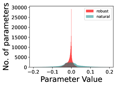
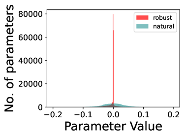
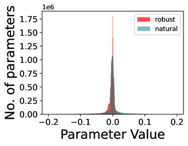
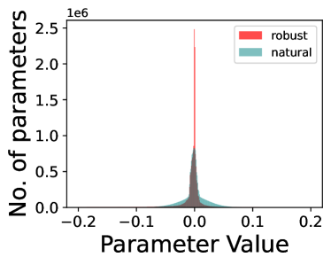
For example, figure 1 shows the weight distribution of networks trained to minimize verified robust (CROWN-IBP (Zhang et al. 2020)) and natural losses. As evident from the distribution of weights, a higher fraction of weights in verified robust models have very low magnitudes ($\approx 10^{-40}$).

This observation suggests that minimizing the loss $\mathcal{L}_{\text{train}}$ bounding by CROWN-IBP penalizes the network parameter magnitudes. Existing sparse training approaches (Louizos, Welling, and Kingma 2018; He et al. 2020) used regularization terms in their loss function to promote sparsity. Since the $\mathcal{L}_{\text{train}}$ implicitly incorporates regularization, VeriCompress does not include any additional regularization term.

Parameter Deactivation based on Element Importance

This step considers the importance of a node/kernel as a whole as the deciding factor for its state. All the parameters associated with the least significant nodes/kernels are set to zero. VeriCompress uses $\ell_{2}$-norm (following (He et al. 2018)) of all the parameter weights corresponding to a kernel or node to decide the indices of kernels/nodes to be deactivated from a layer. Since the kernels/nodes belonging to different layers have different numbers of parameters associated with them, the norm of these kernels/nodes are not comparable globally (Pytorch 2020). Therefore, the deactivation process is applied layer-wise.

Thus, if $m_{i}$ represents the $i$th kernel/node of layer $l$ and $m_{i,j}$ represents $j^{th}$ parameter associated with it, element deactivation can be formulated as: $\theta_{l}^{\downarrow}=[m_{i}|m_{i}\in p_{l}^{th}\text{ percentile of }\sqrt{\sum_{j}m_{i,j}^{2}}],$ and $\theta_{l}-\theta_{l}^{\downarrow}=0,$ where $\theta_{l}^{\downarrow}$ represents active kernel/node retained at layer $l$ after deactivation and $p_{l}$ is the percentage of parameters to be deactivated at layer $l$. The value of $p_{l}$ is decided based on Erdős-Rényi-Kernel scaling (used in (Evci et al. 2021; Raihan and Aamodt 2020)).

4 Experiments

The following section’s evaluations demonstrate (1) The effectiveness of VeriCompress in achieving verified robust models which outperform the state-of-the-art structured pruning approaches; (2) The scalability and generalizability of VeriCompress with backbone network variations, i.e., with different network complexities and architectures, such as Resnet, ResNext, and DenseNet; (3) The applicability of VeriCompress to a practical application domain; and (4) the reduction in memory, training-time, and inference-time.

Metrics for evaluations: This paper utilizes the metrics used in the previous works for formal robustness verification  (Sehwag et al. 2020; Kang, Li, and Li 2023) to evaluate the compressed models. The metrics are:

1. Standard Accuracy: Percentage of benign samples classified correctly.

2. Verified Accuracy: Percentage of benign samples which are certified to be robust using verified robustness mechanism IBP (Gowal et al. 2018), thus, measures the verified robustness of the model. Details are in Appendix A.

Datasets and Models: For a fair comparison with state-of-the-art (Kang, Li, and Li 2023), benchmark dataset CIFAR-10 (Krizhevsky, Nair, and Hinton 2009) and SVHN (Netzer et al. 2011) are used. To demonstrate the effectiveness and generalizability of VeriCompress, evaluations are shown for two more datasets: MNIST (LeCun and Cortes 2010) and Pedestrian Detection (N J Karthika 2020). To demonstrate the versatility of the approach across different architectures, we evaluate (a) Two CNNs with varying capacity: 4-layer CNN and 7-layer CNN  (Gowal et al. 2018; Zhang et al. 2020); (b) Network with skip connections: A 13-layer ResNet (Wong et al. 2018); (c) Two DNNs: DenseNet and ResNext  (Xu et al. 2020). Notably, the models used in this work are used in state-of-the-art robust training approaches, as cited next to their names.

Perturbation Amount: For image classification datasets, the perturbations are introduced in $\ell_{p}-$ball of radius $\varepsilon$ (perturbation amount), $\mathbb{B}_{p}(x_{0},\varepsilon)$ (defined in Section A). For a fair comparison, while comparing our results with baselines (Sehwag et al. 2020; Kang, Li, and Li 2023), we use the same perturbation budget used in these works: 2/255 for CIFAR-10 and SVHN. For MNIST, we use a $\varepsilon=0.4$, the highest perturbation amount for MNIST (i.e., most difficult scenarios) used in the literature addressing formal verification and training  (Gowal et al. 2018; Zhang et al. 2020; Wong et al. 2018; Xu et al. 2020). For the Pedestrian Detection dataset, we use 2/255 as the perturbation amount.

Hyperparameters: VeriCompress requires a set of hyperparameters as inputs: $\varepsilon-scheduler$ inputs $(T,s,l)$ and exploration length T-exp. $T$ is the total number of training epochs, $s$ is the epoch number at which the perturbation scheduler should start to increment the amount of perturbation, and $l$ specifies the length of the schedule, that is, the number of epochs in which the perturbation scheduler has to reach the maximum amount of perturbation $\varepsilon_{\text{max}}$.

These values are as follows: (1) For SVHN and CIFAR-10, we use $((T,s,l)=(330,15,150)$ (2) For MNIST, we use $((T,s,l)=(100,10,60)$, and (3) For Pedestrian Detection, the hyperparameters $(T,s,l)=(100,20,60)$ resulted in the models displaying the least errors empirically. Notably, using a fixed perturbation amount throughout training results in a trivial model.

To obtain the optimum values for the length of exploration T-exp, Optuna (Akiba et al. 2019), a parameter-tuning tool, is used in order to attain the combined objective of maximizing Standard and Verified accuracy.

Learning-Rate Decay: VeriCompress employs learning rate decay once the perturbation scheduler achieves the maximum perturbation. An initial high learning rate allows the dormant elements a fair chance to be considered toward the sub-network structure during the model exploration.

Formal Verification Mechanisms to Compute $\mathcal{L}_{\text{train}}$ and Verified Accuracy: VeriCompress training employs CROWN-IBP  (Zhang et al. 2020). However, to be consistent with the state-of-the-art  (Sehwag et al. 2020; Kang, Li, and Li 2023), this section’s presented evaluations use IBP to compute Verified accuracy.

Establishing the Effectiveness of VeriCompress: Comparison with Baselines

This section compares the compressed models obtained via VeriCompress with the state-of-the-art approaches: FaShapley (Kang, Li, and Li 2023) (best-baseline) and Hydra (Sehwag et al. 2020). Unfortunately, we could not reproduce the results for FaShapley with the provided code. Therefore, for a fair comparison, this section’s evaluations are done with the same combination of model, dataset, and sparsity amounts as used in FaShalpley (Kang, Li, and Li 2023) and compared with the baseline results as provided in the paper.

Table 1 shows the comparison of VeriCompress with Fashapley and Hydra for two architectures: 4-layer CNN and 7-layer CNN trained for CIFAR-10 and SVHN. The perturbation amount used for training and testing these models is $2/255$. The model size is shown in terms of the number of parameters where M stands for million. The percentage next to the model size represents the compressed model’s size with respect to the backbone architecture. Across all model, dataset, and compression combinations, VeriCompress attains an average increment of $15.1$ and $9.8$ percent points in Standard and Verified accuracy, respectively. The results shown in Table 1 are an average of computations for three seed values followed by their error bars.

	Model	Method	Standard	Verified	Standard	Verified
CIFAR-10	4-layer CNN	Parameters	0.106 M (50%)		0.085 M (40%)
	Size=0.215 M	Hydra	44.2	32.5	32.5	22.0
	Standard/	FaShapley	46.7	36.9	32.1	26.8
	Verified	VeriCompress	52.1 ($\pm$0.31)	42.2 ($\pm$0.15)	50.6 ($\pm$1.86)	41.0 ($\pm$1.93)
	54.3/42.9	$\Delta$	+5.4	+5.3	+18.5	+14.2
	7-layer CNN	Parameters	3.295 M (20%)		1.598 M (10%)
	Size=17.190 M	Hydra	52.1	39.8	10.0	10.0
	Standard/	FaShapley	55.5	43.9	19.5	14.2
	Verified	VeriCompress	59.1 ($\pm$0.55)	44.9 ($\pm$2.72)	55.1 ($\pm$1.27)	43.8 ($\pm$1.22)
	66.3/47.0	$\Delta$	+3.6	+1.0	+35.6	+29.6
SVHN	4-layer CNN	Parameters	0.106 M (50%)		0.065 M (30%)
	Size=0.215 M	Hydra	47.8	33.9	19.6	19.6
	Standard/	FaShapley	49.5	37.2	41.9	32.3
	Verified	VeriCompress	57.8 ($\pm$2.45)	38.8 ($\pm$2.34)	54.9 ($\pm$3.33)	37.5 ($\pm$1.42)
	60.0/41.4	$\Delta$	+8.3	+1.6	+13.0	+5.2
	7-layer CNN	Parameters	3.295 M (20%)		2.239 M (15%)
	Size=17.190 M	Hydra	49.2	34.9	15.9	15.9
	Standard/	FaShapley	60.1	43.6	39.0	32.0
	Verified	VeriCompress	68.7 ($\pm$1.35)	49.4 ($\pm$1.94)	66.9 ($\pm$4.95)	47.7 ($\pm$4.38)
	73.8/55.4	$\Delta$	+8.6	+5.8	+27.9	+15.7

Table 1: Standard and Verified Accuracy for 4-layer CNN and 7-layer CNN trained for CIFAR-10 and SVHN at $\varepsilon=2/255$ for different parameters budgets (corresponding to structured pruning amounts used in the baseline). $\Delta$ represents the change as compared to the best baseline, M stands for million parameters

Establishing the Wider Applicability

This section demonstrates the applicability and scalability of VeriCompress by evaluating various backbone network architectures, complexities, and datasets. Evaluation results are discussed below:

$\bullet$ Evaluation for Complex Models: To demonstrate the scalability of VeriCompress to more complex backbone network architectures, we compute compressed models for Resnet, DenseNet, and ResNext (used by (Xu et al. 2020)) on the CIFAR-10 dataset. Table 2 shows that VeriCompress extracted compressed models’ performance in comparison to their dense counterparts is comparable to the Table 1 evaluation results, showing VeriCompress performs similarly across different network complexities and architectures.

Model	Standard	Verified	Standard	Verified	Standard	Verified
Resnet	4.213 M (100%)		0.799 M (20%)		0.398 M (10%)
	57.2	46.0	55.0	44.1	51.0	41.5
DenseNet	7.897 M (100%)		1.667 M (20%)		0.914 M (10%)
	57.7	46.8	56.5	45.3	49.2	38.9
ResNeXt	17.591 M (100%)		3.330 M (20%)		1.714 M (10%)
	58.5	46.7	58.2	46.5	45.8	37.2

Table 2: Comparison of compressed models obtained using VeriCompress for Resnet, DenseNet and ResNeXt trained for CIFAR-10 at $\varepsilon=2/255$ with their dense counterparts.

$\bullet$ Evaluations for more Datasets: This section evaluates VeriCompress’s generalizability on MNIST and Pedestrian Detection). Table 3 demonstrates the results for additional image datasets: (a) a pedestrian detection dataset that aims at differentiating between people and people-like objects (N J Karthika 2020), and (b) MNIST. The backbone architecture used for these evaluations is a 7-layer CNN, adapted to the respective datasets. For both datasets, the performance of the compressed models is comparable to that of their dense counterparts. The perturbation amount used for Pedestrian Detection and MNIST are $2/255$, and $0.4$.

Dataset	Standard	Verified	Standard	Verified	Standard	Verified
Pedestrian	321.5 M (100%)		122.6 (40%)		90.5 M (30%)
Detection	71.6	36.5	71.1	33.6	68.7	24.2
MNIST	1.97 M (100%)		0.94 M (50%)		0.74 M (40%)
	97.7	87.8	95.4	82.2	95.1	80.1

Table 3: Comparison of compressed models obtained using VeriCompress using 7-layer CNN as backbone architecture trained for (a) Pedestrian Detection $(\varepsilon=2/255)$ and (b) MNIST $(\varepsilon=0.4)$

Training and Inference Resource Reduction

This section evaluates the training and inference time, and resource reduction through the VeriCompress extracted compressed NNs, compared to their dense counterparts and baselines.

Method $\Rightarrow$	Hydra	FaShapely	VeriCompress
4-layer CNN	9.2	9.0	3.4
7-layer CNN	20.9	18.8	7.5

Table 4: Training Time (in Ksec) for Hydra, FaShapley and VeriCompress

Reduction in Training Time for VeriCompress’s Compressed Network Extraction Compared to the Baselines:

VeriCompress requires almost one-third of clock-time as that of the pruning-based baselines (Sehwag et al. 2020; Kang, Li, and Li 2023). Table 4 compares the training time required by Hydra (Sehwag et al. 2020), FaShapley (Kang, Li, and Li 2023) and VeriCompress for 4-layer CNN and 7-layer CNN trained for CIFAR-10, while using the same number of training epochs. That is, the total number of epochs used in pre-training, pruning, and fine-tuning for state-of-the-art (Sehwag et al. 2020; Kang, Li, and Li 2023) and an equal number of epochs for VeriCompress. These training times are computed for NVIDIA RTX A6000.

Model	Compression $\Rightarrow$	0%	90%
7-layer CNN	Inference Time(ms)	6.4	3.5
	Memory(MB)	68.8	13.7
	Peak CPU usage (%)	55	51
	Peak RAM usage(Mb)	98	60
Resnet	Inference Time(ms)	4.54	0.81
	Memory(MB)	16.9	2.07
	Peak CPU usage(%)	54	51
	Peak RAM usage(Mb)	50	37

Table 5: Comparison of inference time per sample and resource requirements for compressed models for 7-layer CNN and Resnet trained for CIFAR-10 with their dense counterparts on Google Pixel 6

Real-deployment Evaluations on the Reduction in Time and Memory Requirement of Compressed Models:

VeriCompress’s compressed models result in memory and inference time reductions in the resource constraint generic platforms. Table 5 compares compressed models with their dense counterparts on Google Pixel 6, which has 8GB RAM, powered by a 2.8GHz octa-core Google Tensor processor, running on an Android 12.0 system.

The inference time shown in Table 5 is computed as the average over the result of three experiment trials, which computes the average time required per sample over 10,000 repetitions. It is observed that compressed 7-layer CNN and Resnet require about $5-8$ times less memory, $2-4$ times less inference time, and significantly less RAM used by their dense counterparts. These evaluations demonstrate the impact of VeriCompress in enabling resource-constraint generic platforms to leverage verified robust models. However, the resource reductions come at the cost of reduced generalizability which is discussed in Appendix D.

5 Real World Deployment Scope and Impact

Medical diagnosis and other safety-critical applications such as autonomous driving need a guarantee of accurate inferences while having a model complying with memory constraint (Lederer et al. 2022). However, training such compressed NN models using state-of-the-art structured pruning approaches requires in-depth knowledge of pruning and extensive computation resources. In addition, tuning a large number of hyper-parameters during training and network structure identification increases the computation time exponentially. This complexity might not be practical for end-users, including developers in domains like internet-of-things (IoT), embedded systems, or medical applications. Following VeriCompress’s traits make it a viable solution for such scenarios :

$\bullet$ Automates the learning of compressed models: VeriSprase enables the user to give as input a complex model architecture and a parameter budget that depends on the memory constraint of the deployment platform and generates a compressed model which exhibits high verified robustness. Thus, the user doesn’t need the expertise of model pruning mechanisms to achieve the compressed model.

$\bullet$ Faster training: Notably, the training time of the VeriCompress approach is $2-3$ times less than the baseline structured pruning approaches. Furthermore, VeriCompress computes the importance of a model element (kernel/node) using the magnitude of its parameters, which is data independent; thus, requires significantly less computation as compared to state-of-the-art approaches that rely on specific data-dependent importance scores training phases.

$\bullet$ Fewer hyper-parameters to tune: In addition to common hyper-parameters such as batch size, learning rate, etc., verified robustness approaches generally require hyper-parameters such as the number of epochs and start-and-end of perturbation scheduler. State-of-the-art structured pruning approaches Hydra and Fashapley need to tune these hyperparameters for 3 phases: pre-training, pruning, and finetuning. In contrast, VeriCompress reduces that to a single phase.

6 Conclusion

This paper presents VeriCompress - a tool designed to streamline the synthesis of compressed verified robust NNs from scratch, leveraging relatively less computation, time, and effort than the state-of-the-art literature. Our empirical evaluations demonstrate the effectiveness of VeriCompress in achieving compressed networks of the required size while exhibiting generalizability comparable to its dense counterparts. The practical deployment of these resultant models onto a resource-constraint generic platform effectively demonstrates reductions in both memory and computational demands. The accelerated generation process, broader applicability, and effectiveness of VeriCompress will greatly assist users such as edge, embedding systems, or IoT developers in effortlessly generating and deploying verified robust compressed models tailored for their respective safety-critical and resource-constrained generic platforms.

Appendix A A. Background and Related-Works

Background on Formal robustness verification

An NP-Complete problem: The complexity and the need for non-linear activation functions in recent NNs to learn complex decision boundaries makes the problem of formal robustness verification of NNs non-convex and NP-Complete  (Katz et al. 2017).

Relaxation-based Methods: To address the challenge, Katz et al. (2017) used relaxation of ReLU activations, temporarily violating the ReLU semantics, resulting in an efficient query solver for NNs with ReLU activations. The piece-wise linearity of the ReLU activations is the basis for this relaxation. Linear Relaxation-based Perturbation Analysis (LiRPA) based methods compute the linear relaxation of a model containing general activation functions which are not necessarily piece-wise linear and verify non-linear NNs in polynomial time. Thus, LiRPA-based methods use Forward (IBP (Gowal et al. 2018)), Backward (CROWN (Zhang et al. 2018), Fastened-CROWN (Lyu et al. 2020)) or Hybrid (CROWN-IBP (Zhang et al. 2020)) bounding mechanisms to compute linear relaxation of a model. CROWN (Zhang et al. 2018) uses a backward bounding mechanism to compute linear or quadratic relaxation of the activation functions. IBP (Gowal et al. 2018) is a forward bounding mechanism that propagates the perturbations induced to the input towards the output layer in a forward pass based on interval arithmetic, resulting in ranges of values for each class in the output layer. CROWN-IBP (Zhang et al. 2020) is a hybrid approach that demonstrated that IBP can produce loose bounds, and to achieve tighter bounds, it uses IBP  (Gowal et al. 2018) in the forward bounding pass and CROWN (Zhang et al. 2018) in the backward bounding pass to compute bounding hyperplanes for the model. CROWN-IBP has been shown to compute tighter relaxations, thus, providing better results for formal verification.

Specifically, for a sample $x_{0}$, the perturbation neighborhood is defined as $\ell_{p}$-ball of radius $\varepsilon$ (Zhang et al. 2018):

$$\mathbb{B}_{p}(x_{0},\varepsilon):=\{x|\|x-x_{0}\|_{p}\leq\varepsilon\}.$$ (2)

LiRPA aims to compute linear approximations $f^{\varepsilon}$ of the model $\mathcal{M}_{\theta}$ ($\theta$ represents model parameters), and provide lower $f_{L}^{\varepsilon}$ and upper $f_{U}^{\varepsilon}$ bounds at the output layer, such that for any sample $x\in\mathbb{B}_{p}(x_{0},\varepsilon)$ and each class $j$, the model output is guaranteed to follow:

$$f_{L}^{\varepsilon}(x)^{j}\leq\mathcal{M}_{\theta}(x)^{j}\leq f_{U}^{\varepsilon}(x)^{j}.$$ (3)

Background on Verified robustness.

A NN model, $\mathcal{M}_{\theta}$ is said to be verified robust  (Fromherz et al. 2021) for a sample $(x_{0},y)$ if: $\forall x\in\mathbb{B}_{p}(x_{0},\varepsilon)\Rightarrow\mathcal{M}_{\theta}(x)=\mathcal{M}_{\theta}(x_{0})$, that is, for all the samples $x\in\mathbb{B}_{p}(x_{0},\varepsilon)$, the model is guaranteed to assign the same class as it assigns to $x_{0}$. LiRPA approaches measure the robustness in terms of a margin vector $m(x_{0},\varepsilon)=Cf^{\varepsilon}(x_{0})$, where C is a specification matrix of size $n\times n$ and $n$ is the number of all possible classes (Gowal et al. 2018; Zhang et al. 2018, 2020; Xu et al. 2020). Zhang et al. (2020) defines $C$ for each sample $(x_{0},y)$ as:

$$C_{i,j}=\begin{cases}1,&j=y\text{ and }i\neq y\text{ (truth class)}\\ -1,&i=j\text{ and }i\neq y\text{ (other classes)}\\ 0,&\text{ otherwise}.\end{cases}$$ (4)

The entries in matrix $C$ depend on the true class $y$. In matrix $C$, the row corresponding to the true class contains $0$ at all the indices. All the other rows contain $1$ at the index corresponding to the true class $(j=y)$ and $-1$ at the index corresponding to current class $(j=i)$ and $0$ at all the other indices. Thus, the $i^{th}$ value of $m(x_{0},\varepsilon)$ is given by $m^{i}(x_{0},\varepsilon)=f^{\varepsilon}(x_{0})^{y}-f^{\varepsilon}(x_{0})^{i}$, which is the difference of output values of the true class $y$ from the output value corresponding to class $i$.

Further, $\underline{m}(x_{0},\varepsilon)$ represents the lower bound of the margin vector. If all the values of the $\underline{m}(x_{0},\varepsilon)$ are positive, $\forall_{i\neq y}\underline{m}^{i}(x_{0},\varepsilon)>0$, the model $\mathcal{M}_{\theta}$ is said to be robust for sample $x_{0}$. That implies, the model will always assign the highest output value to the true class label $y$ if a perturbation less than or equal to $\varepsilon$ is induced to the sample $x_{0}$. Thus, $\forall_{j}\underline{m}(x_{0},\varepsilon)^{j}>0$ implies the guaranteed absence of any adversarial sample in the region of interest. Furthermore, to specify the region bounded by $\mathbb{B}_{p}(x_{0},\varepsilon)$ , we use $p=\infty$ because $\ell_{\infty}$-norm covers the largest region around a sample and is most challenging and widely-used (Kang, Li, and Li 2023; Wong and Kolter 2018).

Background on Model training to maximize robustness

Since a model is considered verified robust for a sample $(x_{0},y)$ if all the values of $\underline{m}(x_{0},\varepsilon)>0$, the training schemes proposed by previous approaches (Gowal et al. 2018; Zhang et al. 2020) aim to maximize robustness of a model by maximizing the lower bound $\underline{m}(x_{0},\varepsilon)$. Xu et al. (2020) defines the training objective as minimizing the maximum cross-entropy loss between the model output $\mathcal{M}_{\theta}(x)$ and the true label $y$ among all samples $x\in\mathbb{B}_{p}(x_{0},\varepsilon)$ (eq. 6 in  (Xu et al. 2020)). Thus, the training loss is defined as:

$$\mathcal{L}_{\text{train}}(\mathcal{M}_{\theta},\mathcal{D},\varepsilon)=\sum_{(x_{0},y)\in\mathcal{D}}\max_{x\in\mathbb{B}(x_{0},\varepsilon)}\mathcal{L}(\mathcal{M}_{\theta}(x),y),$$ (5)

where $\mathcal{D}$ is the dataset and $(x_{0},y)\in\mathcal{D}$. Intuitively, $\mathcal{L}_{\text{train}}$ is the sum of maximum cross-entry loss in the neighborhood of each sample in $\mathcal{D}$ for perturbation amount $\varepsilon$. Wong and Kolter (2018) showed that the problem of minimizing $\mathcal{L}_{\text{train}}$ (as defined in 5) and the problem of maximizing $\underline{m}(x_{0},\varepsilon)$ are dual of each other. Thus, a solution that minimizes $\mathcal{L}_{\text{train}}$, maximizes the values of $\underline{m}(x_{0},\varepsilon)$, hence maximizes the robustness for the sample $(x_{0},y)$. Since, $x_{0}\in\mathbb{B}_{p}(x_{0},\varepsilon)$, minimizing $\mathcal{L}_{\text{train}}$ also maximizes benign/standard accuracy, ergo maximizes generalizability altogether.

Xu et al. (2020) computes $\max_{x\in\mathbb{B}(x_{0},\varepsilon)}\mathcal{L}(\mathcal{M}_{\theta}(x),y)$ which requires computing bounding hyper-planes $f_{U}^{\varepsilon}$ and $f_{L}^{\varepsilon}$ using one of the aforementioned LiRPA bounding techniques. Following Xu et al. (2020), VeriCompress employs CROWN-IBP hybrid approach as the bounding mechanism to optimize $\mathcal{L}_{\text{train}}(\mathcal{M}_{\theta},\mathcal{D},\varepsilon)$ in equation (5). The perturbation amount $\varepsilon$ is initially set to zero and gradually increases to $\varepsilon_{\text{max}}$ according to the perturbation scheduler $\varepsilon$-scheduler$(\varepsilon_{\text{max}},t,s,l)$ (Section 3).

$\bullet$ Perturbation Scheduler $(\varepsilon$-scheduler ($\varepsilon_{\text{max}},t,s,l)$:

$\varepsilon$-scheduler provides a perturbation amount for every training epoch $t\geq s$, which gradually increases $\varepsilon$ starting at epoch s. The schedule starts with a 0 perturbation and reaches $\varepsilon_{\text{max}}$ in $l$ epochs (Gowal et al. 2018). According to the literature (Gowal et al. 2018; Zhang et al. 2020; Xu et al. 2020), the Linear Relaxation-based Perturbation Anaysis (LiRPA) approaches use interval propagation arithmetic to propagate input perturbation to the output layer, where the interval size usually keeps increasing as the propagations reach deeper in the model. This issue is known as the problem of intermediate-bound explosion. A perturbation scheduler helps deal with this issue by gradually increasing the perturbation amount.

Appendix B Model Compression

While various compression techniques are available, to the best of our knowledge, only model pruning approaches have been leveraged to achieve verified robust compressed models in the literature  (Sehwag et al. 2020; Kang, Li, and Li 2023). Consequently, the focus of this section is confined to pruning discussions. Furthermore, given that VeriCompress adopts the Dynamic Sparse Training (DST) approach, a discussion on DST is also included.

Model Pruning

Model pruning approaches train a dense model to convergence and remove (or prune) the parameters, either in one step or iteratively, which contribute the least towards model inference. To compensate for the information lost during pruning, an additional step of fine-tuning the retained parameters is performed by associating a static binary mask with the parameters. The removal of parameters can be done at different granularity: unstructured pruning (fine-grained) and structured pruning (coarse-grained).

Structured vs. Unstructured Pruning

Unstructured pruning zeros out the parameters depending on their individual importance (Sehwag et al. 2020), whereas structured pruning removes channels/nodes as a whole (Phan et al. 2022). It has been observed that structured pruning is effective in significantly reducing memory and inference time in generic platforms, making them highly effective in practical use (Sadou et al. 2022).

Selecting the Parameters to be Removed during Sparsification:

Selection of parameters to be removed can be done based on several criteria such as the magnitude of weights (Sehwag et al. 2019), the norm of corresponding gradients (Molchanov et al. 2017), etc. Additionally, recent approaches associate importance scores with each parameter based on the respective training objective (Sehwag et al. 2020; Kang, Li, and Li 2023), and remove the parameters with the least important scores. Presented VeriCompress exceeds state-of-the-art without any task/objective specific important score-based parameter selection mechanism, establishing that a compressed network with high verified local robustness and accuracy comparable to its dense counterpart is attainable from scratch following trivial parameter selection mechanism.

Dynamic Sparse Training

Recently developed dynamic-mask-based sparse-training known as Dynamic Sparse Training (DST) (Dai, Yin, and Jha 2019; Liu et al. 2021) approaches follow grow-and-prune paradigm to achieve a favorable sparse network starting from a random sparse seed network. Dai, Yin, and Jha (2019) grows the model to a certain capacity and then gradually removes the connection, following a single grow-and-prune stride. However, recent approaches (Liu et al. 2021) employ multiple repetitions of grow-and-prune where, in each repetition, new connections (i.e., parameters) which minimize the natural loss are added, and the least important connections are removed.

Appendix C Code

The code is available at https://github.com/Sawinder-Kaur/VeriCompress.

Appendix D Cost-Benerfit Analysis

It is evident from Table 1 (Section 4) that while the presented VeriCompress approach surpasses existing methods, reducing the number of parameters still negatively impacts model performance, which is measured in terms of accuracy and verified robustness. For instance, for 7-layer CNN trained for CIFAR10, when the number of parameters is reduced from 17.19 M to 3.26M (approximately 5 times reduction than the over-parameterized model), the accuracy and verified robustness reduces by 6.4% and 2.1% respectively. However, a reduction to 1.58M (approximately 10 times reduction than the over-parameterized model) results in a drop of 11.2% in accuracy and 3.2% in verified robustness. Additionally, this drop varies with the complexity and the architecture of the backbone model. Notably, as shown in Table 4 (Section 4) of the main paper, fewer parameters lead to smaller-sized models and reduced inference time. Thus resulting in efficient models. For instance, reducing the parameters of the 7-layer to one-tenth reduces the memory requirement to one-fifth and inference time to half.

(a) 4-layer CNN (CIFAR-10)

(b) 7-layer CNN (CIFAR-10)

(c) 4-layer CNN (SVHN)

(d) 7-layer CNN (SVHN)

Figure 2: Cost Benefit Analysis for (a) 4-layer CNN (CIFAR10) (b) 4-layer CNN (CIFAR-10) (b) 4-layer CNN (SVHN) (d) 7-layer CNN (SVHN). The pertubation amount used for robust training is 2/255.

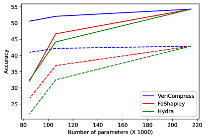
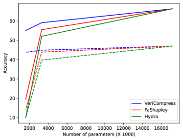
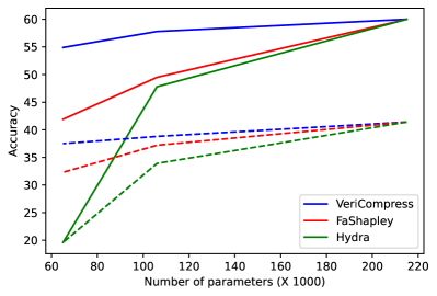
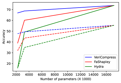
Figure 2 showcases the superior performance of the VeriCompress approach over the baselines. The figure discusses the cost-benefit analysis for a 4-layer CNN and 7-layer CNN trained for CIFAR-10 and SVHN. The solid and dotted lines represent the accuracy and verified robustness of the model. It’s evident that while the presented VeriCompress approach surpasses existing methods, reducing the number of parameters still negatively affects model performance, as measured by accuracy and verified robustness.

This underscores the existence of a trade-off between model efficiency and performance. Consequently, the choice between prioritizing high performance or enhanced efficiency depends on the specific application requirements and the available resources on the deployment platform.

References

- Akiba et al. (2019) Akiba, T.; Sano, S.; Yanase, T.; Ohta, T.; and Koyama, M. 2019. Optuna: A Next-generation Hyperparameter Optimization Framework. ISBN 978-1-4503-6201-6.
- Dai, Yin, and Jha (2019) Dai, X.; Yin, H.; and Jha, N. K. 2019. NeST: A Neural Network Synthesis Tool Based on a Grow-and-Prune Paradigm. IEEE Transactions on Computers, 68(10): 1487–1497.
- Evci et al. (2021) Evci, U.; Gale, T.; Menick, J.; Castro, P. S.; and Elsen, E. 2021. Rigging the Lottery: Making All Tickets Winners. arXiv:1911.11134.
- Evci et al. (2022) Evci, U.; Ioannou, Y.; Keskin, C.; and Dauphin, Y. 2022. Gradient Flow in Sparse Neural Networks and How Lottery Tickets Win. Proceedings of the AAAI Conference on Artificial Intelligence, 36(6): 6577–6586.
- Fang et al. (2023) Fang, G.; Ma, X.; Song, M.; Mi, M. B.; and Wang, X. 2023. DepGraph: Towards Any Structural Pruning. arXiv:2301.12900.
- Fromherz et al. (2021) Fromherz, A.; Leino, K.; Fredrikson, M.; Parno, B.; and Pasareanu, C. 2021. Fast Geometric Projections for Local Robustness Certification. In International Conference on Learning Representations.
- Goodfellow, Shlens, and Szegedy (2015) Goodfellow, I. J.; Shlens, J.; and Szegedy, C. 2015. Explaining and Harnessing Adversarial Examples. CoRR, abs/1412.6572.
- Gowal et al. (2018) Gowal, S.; Dvijotham, K.; Stanforth, R.; Bunel, R.; Qin, C.; Uesato, J.; Arandjelović, R.; Mann, T. A.; and Kohli, P. 2018. On the Effectiveness of Interval Bound Propagation for Training Verifiably Robust Models. ArXiv, abs/1810.12715.
- Guo et al. (2023) Guo, L. L.; Steinberg, E.; Fleming, S. L.; Posada, J.; Lemmon, J.; Pfohl, S. R.; Shah, N.; Fries, J.; and Sung, L. 2023. EHR foundation models improve robustness in the presence of temporal distribution shift. Scientific Reports, 3767.
- He et al. (2020) He, J.; Jia, X.; Xu, J.; Zhang, L.; and Zhao, L. 2020. Make L1 regularization effective in training sparse CNN. Computational Optimization and Applications, 77(1): 163– 182.
- He et al. (2018) He, Y.; Kang, G.; Dong, X.; Fu, Y.; and Yang, Y. 2018. Soft Filter Pruning for Accelerating Deep Convolutional Neural Networks. arXiv:1808.06866.
- Julian et al. (2019) Julian, K. D.; Sharma, S.; Jeannin, J.-B.; and Kochenderfer, M. J. 2019. Verifying Aircraft Collision Avoidance Neural Networks Through Linear Approximations of Safe Regions. arXiv:1903.00762.
- Kang, Li, and Li (2023) Kang, M.; Li, L.; and Li, B. 2023. FaShapley: Fast and Approximated Shapley Based Model Pruning Towards Certifiably Robust DNNs. In First IEEE Conference on Secure and Trustworthy Machine Learning.
- Katz et al. (2017) Katz, G.; Barrett, C.; Dill, D. L.; Julian, K.; and Kochenderfer, M. J. 2017. Reluplex: An Efficient SMT Solver for Verifying Deep Neural Networks. In Majumdar, R.; and Kunčak, V., eds., Computer Aided Verification, 97–117. Springer International Publishing. ISBN 978-3-319-63387-9.
- Kim, Park, and Ro (2021) Kim, J. U.; Park, S.; and Ro, Y. M. 2021. Robust Small-scale Pedestrian Detection with Cued Recall via Memory Learning. In 2021 IEEE/CVF International Conference on Computer Vision (ICCV), 3030–3039.
- Krizhevsky, Nair, and Hinton (2009) Krizhevsky, A.; Nair, V.; and Hinton, G. 2009. Learning multiple layers of features from tiny images.
- LeCun and Cortes (2010) LeCun, Y.; and Cortes, C. 2010. MNIST handwritten digit database.
- Lederer et al. (2022) Lederer, A.; Zhang, M.; Tesfazgi, S.; and Hirche, S. 2022. Networked Online Learning for Control of Safety-Critical Resource-Constrained Systems based on Gaussian Processes. In 2022 IEEE Conference on Control Technology and Applications (CCTA), 1285–1292.
- Liu et al. (2021) Liu, S.; Yin, L.; Mocanu, D. C.; and Pechenizkiy, M. 2021. Do We Actually Need Dense Over-Parameterization? In-Time Over-Parameterization in Sparse Training. In Meila, M.; and Zhang, T., eds., Proceedings of the 38th International Conference on Machine Learning, volume 139 of Proceedings of Machine Learning Research. PMLR.
- Louizos, Welling, and Kingma (2018) Louizos, C.; Welling, M.; and Kingma, D. P. 2018. Learning Sparse Neural Networks through L0 Regularization. In International Conference on Learning Representations.
- Lyu et al. (2020) Lyu, Z.; Ko, C.-Y.; Kong, Z.; Wong, N.; Lin, D.; and Daniel, L. 2020. Fastened CROWN: Tightened Neural Network Robustness Certificates. ArXiv, abs/1912.00574.
- Madry et al. (2018) Madry, A.; Makelov, A.; Schmidt, L.; Tsipras, D.; and Vladu, A. 2018. Towards Deep Learning Models Resistant to Adversarial Attacks. In International Conference on Learning Representations.
- Molchanov et al. (2017) Molchanov, P.; Tyree, S.; Karras, T.; Aila, T.; and Kautz, J. 2017. Pruning Convolutional Neural Networks for Resource Efficient Inference. In 5th International Conference on Learning Representations, ICLR 2017, Toulon, France, April 24-26, 2017, Conference Track Proceedings. OpenReview.net.
- N J Karthika (2020) N J Karthika, C. S. 2020. Addressing False Positives in Pedestrian Detection. In International Conference on Electronic Systems and Intelligent Computing (ESIC 2020).
- Netzer et al. (2011) Netzer, Y.; Wang, T.; Coates, A.; Bissacco, A.; Wu, B.; and Ng, A. Y. 2011. Reading Digits in Natural Images with Unsupervised Feature Learning. In NIPS Workshop on Deep Learning and Unsupervised Feature Learning 2011.
- Pereira and Thomas (2020) Pereira, A.; and Thomas, C. 2020. Challenges of Machine Learning Applied to Safety-Critical Cyber-Physical Systems. Machine Learning and Knowledge Extraction, 2(4).
- Phan et al. (2022) Phan, H.; Yin, M.; Sui, Y.; Yuan, B.; and Zonouz, S. 2022. CSTAR: Towards Compact and STructured Deep Neural Networks with Adversarial Robustness.
- Pytorch (2020) Pytorch. 2020. Global structured pruning. https://discuss.pytorch.org/t/global-structured-pruning/67263.
- Raihan and Aamodt (2020) Raihan, M. A.; and Aamodt, T. M. 2020. Sparse Weight Activation Training. arXiv:2001.01969.
- Sadou et al. (2022) Sadou, I.-I.; Nabavinejad, S. M.; Lu, Z.; and Ebrahimi, M. 2022. Inference Time Reduction of Deep Neural Networks on Embedded Devices: A Case Study. In 2022 25th Euromicro Conference on Digital System Design (DSD), 205–213.
- Sehwag et al. (2019) Sehwag, V.; Wang, S.; Mittal, P.; and Jana, S. 2019. Towards Compact and Robust Deep Neural Networks. preprint arXiv:1906.06110.
- Sehwag et al. (2020) Sehwag, V.; Wang, S.; Mittal, P.; and Jana, S. 2020. HYDRA: Pruning Adversarially Robust Neural Networks. 34th Conference on Neural Information Processing Systems.
- Wong and Kolter (2018) Wong, E.; and Kolter, Z. 2018. Provable Defenses against Adversarial Examples via the Convex Outer Adversarial Polytope. In Dy, J.; and Krause, A., eds., Proceedings of the 35th International Conference on Machine Learning, volume 80 of Proceedings of Machine Learning Research, 5286–5295. PMLR.
- Wong et al. (2018) Wong, E.; Schmidt, F.; Metzen, J. H.; and Kolter, J. Z. 2018. Scaling provable adversarial defenses. In Bengio, S.; Wallach, H.; Larochelle, H.; Grauman, K.; Cesa-Bianchi, N.; and Garnett, R., eds., Advances in Neural Information Processing Systems, volume 31. Curran Associates, Inc.
- Xu et al. (2020) Xu, K.; Shi, Z.; Zhang, H.; Wang, Y.; Chang, K.-W.; Huang, M.; Kailkhura, B.; Lin, X.; and Hsieh, C.-J. 2020. Automatic Perturbation Analysis for Scalable Certified Robustness and Beyond. In Proceedings of the 34th International Conference on Neural Information Processing Systems, NIPS’20. Red Hook, NY, USA: Curran Associates Inc. ISBN 9781713829546.
- Zhang et al. (2020) Zhang, H.; Chen, H.; Xiao, C.; Gowal, S.; Stanforth, R.; Li, B.; Boning, D. S.; and Hsieh, C. 2020. Towards Stable and Efficient Training of Verifiably Robust Neural Networks. In 8th International Conference on Learning Representations, ICLR 2020, Ethiopia, April 26-30, 2020.
- Zhang et al. (2018) Zhang, H.; Weng, T.-W.; Chen, P.-Y.; Hsieh, C.-J.; and Daniel, L. 2018. Efficient Neural Network Robustness Certification with General Activation Functions. ArXiv, abs/1811.00866.