Distributed Deep Joint Source-Channel Coding over a Multiple Access Channel

Abstract

We consider distributed image transmission over a noisy multiple access channel (MAC) using deep joint source-channel coding (DeepJSCC). It is known that Shannon’s separation theorem holds when transmitting independent sources over a MAC in the asymptotic infinite block length regime. However, we are interested in the practical finite block length regime, in which case separate source and channel coding is known to be suboptimal. We introduce a novel joint image compression and transmission scheme, where the devices send their compressed image representations in a non-orthogonal manner. While non-orthogonal multiple access (NOMA) is known to achieve the capacity region, to the best of our knowledge, non-orthogonal joint source-channel coding (JSCC) scheme for practical systems has not been studied before. Through extensive experiments, we show significant improvements in terms of the quality of the reconstructed images compared to orthogonal transmission employing current DeepJSCC approaches particularly for low bandwidth ratios. We publicly share source code to facilitate further research and reproducibility.

I Introduction

Conventional wireless communication systems consist of two different stages, called source coding and channel coding. Source coding compresses a signal by removing inherent redundancies. Afterwards, channel coding introduces structured redundancy to improve reliability against channel’s corrupting effects, such as noise and fading. The receiver has to revert these steps by employing a channel decoder and a source decoder, respectively. For instance, wireless image transmission systems employ JPEG or BPG compression to reduce the required communication resources at the expense of reduced reconstructed image quality. The system then employs channel coding, such as LDPC, turbo codes, or polar coding for reliable transmission over a noisy channel. Figure 1 illustrates the conventional separation-based system design for wireless data transmission.

Shannon proved that such a separate design is without loss of optimality when the source and channel block lengths are infinite [1]. However, optimality of separation fails in the practical finite block length regime, or in multi-user networks in general [2]. Moreover, suboptimality gap of separation increases as the block length gets shorter or the signal-to-noise ratio (SNR) diminishes, which correspond to the operation of many delay-sensitive applications such as Internet of Things (IoT) or autonomous driving.

Although researchers have been investigating joint source-channel coding (JSCC) schemes for many decades [3, 4, 5], these schemes did not find application in practical systems due to their high complexity, and poor performance with practical sources and channel distributions. Research on JSCC has gained renewed interest recently with the adoption of deep neural networks (DNNs) to implement JSCC [6]. This data-driven approach is based on modeling the end-to-end communication system as an autoencoder architecture. Numerous follow-up studies have extended deep joint source-channel coding (DeepJSCC) in different directions. In [7], the authors demonstrate that DeepJSCC can exploit feedback to improve the end-to-end reconstruction quality. In [8], DeepJSCC architecture is modified by increasing the filter size to improve the performance. In [9], it is shown that DeepJSCC can adopt to varying channel bandwidth with almost no loss in performance. In addition to very promising results achieved for a particular channel quality, it is worth noting that DeepJSCC avoids the cliff effect suffered by separate source and channel coding and achieves graceful degradation with the channel quality; that is the image is still decodable even when the channel quality falls below the target SNR the system is designed for, albeit with lower quality. Separation-based schemes, on the other hand, completely fail as the channel code cannot be decoded below a certain SNR threshold.

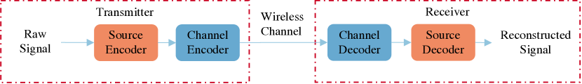
(a)

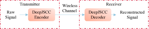
(b)

Figure 1: Separation and DeepJSCC-based data transmission schemes

In this paper, we consider transmission of distinct images over a multiple access channel (MAC). It is known that separation theorem applies to MACs with independent sources; however, the design of practical JSCC schemes for finite block lengths and real information sources remain as an open challenge. A straightforward approach is to employ time division multiple access (TDMA), where each user employs the same trained DeepJSCC network to transmit using half of the channel bandwidth. However, our goal in this work is to develop a DeepJSCC framework that can exploit non-orthogonal communications. A related NOMA-aided JSCC scheme is considered for collaborative inference over a MAC in [10], where the goal is to retrieve a unique identity rather than reconstructing distinct images.

Our main contributions are summarized as follows:

1. To the best of our knowledge, we introduce the first multi-user DeepJSCC-based image transmission method, exploiting non-orthogonal multiple access (NOMA).

2. We introduce a novel Siamese network-based architecture with device embeddings that allows us to use the same set of parameters for both devices, which will be instrumental in scaling our solution to larger networks.

3. We introduce a training data subsampling methodology, and employ curriculum learning (CL)-based training to further improve the performance.

4. Through an extensive set of experiments, we show that our superposition-based method for NOMA outperforms traditional DeepJSCC with time division for all evaluated SNR conditions. We also show that our method is fair; that is, no significant difference is observed between the performances of the two users.

5. To facilitate further research and reproducibility, we provide the source code of our framework and simulations on github.com/ipc-lab/deepjscc-noma.

II Related Works

In this section, we review the works that we construct our methods upon.

II-A Non-Orthogonal Multiple Access (NOMA)

NOMA is essential in achieving the capacity region of a MAC, whereas orthogonal transmission schemes, such as TDMA, are strictly suboptimal. Please see Fig. 2 for an illustration of the capacity region of a MAC, achievable by NOMA, and the suboptimality of TDMA. Although the signals from different users act as interference to each other, either joint decoding [11], or successive interference cancellation (SIC) with message splitting [12] allows to achieve higher rates and meet the capacity. Recently, there have also been efforts to employ DNNs to implement SIC for NOMA [13, 14, 15]. On the other hand, in DeepJSCC, input signal are directly mapped to channel inputs without imposing any constellation constraints. The continuous-amplitude nature of the transmitted signals is beneficial in achieving graceful degradation with channel quality; however, it also means that the decoder is an estimator, and will always have some noise in its reconstruction. That is, unlike in digital communication, the decoder cannot recover the transmitted codeword perfectly, which means that perfect interference cancellation is not possible.

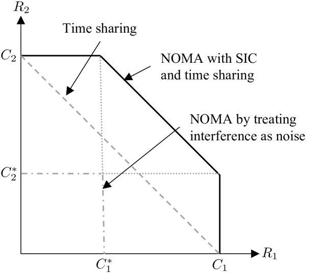
Figure 2: Capacity region of a two-user MAC compared with the rate pairs achievable by TDMA [16].

II-B Related Learning Paradigms: Multi-Task Learning (MTL), Deep Metric Learning (DML) and Curriculum Learning (CL)

MTL is a paradigm of learning multiple tasks jointly to improve performance [17, 18]. In the MAC, multiple signals are superposed onto a joint representation, and the decoder reconstructs multiple images. Therefore, it is inherently a MTL problem. In distributed compression [19], typically different encoding and decoding functions are employed for each of the source signals, which increases the complexity and inhibits scalability. MTL methods often modify feature space or share parameters to improve performance for both tasks [18]. Inspired from these tricks in the MTL literature, we introduce a novel input augmentation embedding for better separability and employ a Siamese neural network-based architecture to reduce the number of parameters [20].

Similarly to DML, our method projects multiple instances into a lower-dimensional latent space with the same network. In DML, typically a subsample of pairs are used for training, and the choice of training pairs significantly affects performance [21]. Therefore, we design a systematic and efficient training methodology instead of using all possible training pairs, which is infeasible.

CL is a progressive training paradigm, where network is first trained on easy tasks and then adapted to the main task of interest [22]. CL has been previously leveraged in [23] by starting training from higher SNRs for progressively adapting to lower SNRs. In our problem, since signals are superposed, they interfere with each other, which affects the training performance. Therefore, we further improve our method by training the network first on non-interfering signals, and then fine-tune it on the actual task.

Notation: Unless stated otherwise; boldface lowercase letters denote vectors (e.g., $\mathbf{p}$), boldface uppercase letters denote matrices (e.g., $\mathbf{P}$), non-boldface letters denote scalars (e.g., $p$ or $P$), and uppercase calligraphic letters denote sets (e.g., ${\cal P}$). $\mathbb{R}$, $\mathbb{N}$, $\mathbb{C}$ denote the set of real, natural and complex numbers, respectively. $|{{\cal P}}|$ denotes the cardinality of set ${\cal P}$. We define $[n]\triangleq\{1,2,\cdots,n\}$, where $n\in\mathbb{N}^{+}$, and $\mathbb{I}\triangleq[255]$.

III System Model

We consider the distributed wireless image transmission problem over a MAC in an uplink setting with two transmitters and a single receiver. Specifically, consider additive white Gaussian noise (AWGN) channel with noise variance $\sigma^{2}$. Transmitter $i$ maps an input image $\mathbf{x}_{i}\in\mathbb{I}^{C_{\mathrm{in}}\times W\times H}$, where $W$ and $H$ denote the width and height of the image, while $C_{\mathrm{in}}$ represents the R, G and B channels for colored images, with a non-linear encoding function $E_{\boldsymbol{\Theta}_{i},\sigma}:\mathbb{I}^{C_{\mathrm{in}}\times W\times H}\rightarrow\mathbb{C}^{k}$ parameterized by $\boldsymbol{\Theta}_{i}$ into a complex-valued latent vector $\mathbf{z}_{i}=E_{\boldsymbol{\Theta}_{i},\sigma}(\mathbf{x}_{i})$, where $k$ corresponds to the available channel bandwidth.

We enforce average transmission power constraint on both transmitters:

$$\frac{1}{k}\left\lVert\mathbf{z}_{i}\right\rVert_{2}^{2}\leq P_{\mathrm{avg}},\,\,i\in\{1,2\}.$$ (1)

The receiver receives the summation of latent vectors as:

$$\mathbf{y}=\mathbf{z}_{1}+\mathbf{z}_{2}+\mathbf{n},$$

where $\mathbf{n}\in\mathbb{C}^{k}$ is independent and identically distributed (i.i.d.) complex Gaussian noise term with variance $\sigma^{2}$, i.e., $\mathbf{n}\sim{\cal C}{\cal N}(\mathbf{0},\sigma^{2}\mathbf{I}_{k})$. We consider $\sigma$ is known at the transmitters and the receiver.

Then, a non-linear decoding function $D_{\boldsymbol{\Phi},\sigma}:\mathbb{C}^{k}\rightarrow\mathbb{I}^{2\times C_{\mathrm{in}}\times W\times H}$ at the receiver, parameterized by $\boldsymbol{\Phi}$, reconstructs both images that are aggregated in the common representation $\mathbf{y}$, i.e.,

$$\begin{bmatrix}\hat{\mathbf{x}}_{1}\\ \hat{\mathbf{x}}_{2}\end{bmatrix}=D_{\Phi,\sigma}(\mathbf{y}).$$

The bandwidth ratio $\rho$ characterizes the available channel resources, and is defined as:

$$\rho=\frac{k}{C_{\mathrm{in}}WH}\,\,$\mathrm{c}\mathrm{h}\mathrm{a}\mathrm{n}\mathrm{n}\mathrm{e}\mathrm{l}\,\mathrm{s}\mathrm{y}\mathrm{m}\mathrm{b}\mathrm{o}\mathrm{l}\mathrm{s}\mathrm{/}\mathrm{p}\mathrm{i}\mathrm{x}\mathrm{e}\mathrm{l}$.$$

We also define the $\mathrm{SNR}$ at time $t$ as:

$$\mathrm{SNR}=10\mathop{\mathrm{log}_{10}\left(\frac{P_{\mathrm{avg}}}{\sigma^{2}}\right)}\,\,$\mathrm{dB}$.$$ (2)

Our objective is to maximize the average peak signal to noise ratio (PSNR), on an unseen target dataset under given channel SNR and the power constraint in (1), which is defined as:

$$\mathrm{PSNR}=10\mathop{\mathrm{log}_{10}\left(\frac{A^{2}}{\frac{1}{C_{\mathrm{in}}HW}\left\lVert\mathbf{x}_{i}-\hat{\mathbf{x}}_{i}\right\rVert_{2}^{2}}\right)}\,\,$\mathrm{dB}$,$$ (3)

where $A$ is the maximum possible input value, e.g., $A=255$ for images with 8-bit per channel as in our case. To achieve this goal, in the next section, we will introduce our framework to implement joint training of the neural network based decoder $D_{\boldsymbol{\Phi},\sigma}$ and encoders $E_{\boldsymbol{\Theta}_{i},\sigma},\,\,i\in\{1,2\}$.

IV Methodology

In this section, we describe our novel methodology to exploit NOMA for efficient image transmission using DeepJSCC. Algorithm 1 summarizes the training methodology of the introduced method, called DeepJSCC-NOMA.

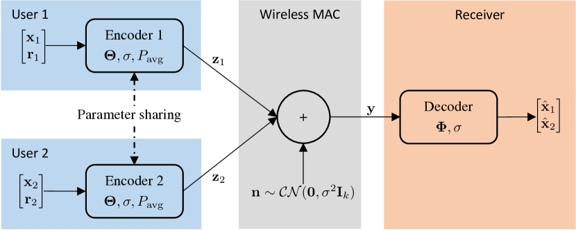
Figure 3: Overall architecture of our DeepJSCC-NOMA method.

IV-A DeepJSCC-NOMA Architecture

Following the practice of previous works [6, 8], we construct our network via an autoencoder-based architecture. We employ the encoder and decoder architectures in [24], removing the quantization part as our method allows continuous channel inputs. It has symmetric encoder and decoder networks with two downsampling/upsampling layers. It utilizes residual connections and the attention mechanism introduced in [25]. It also leverages SNR adaptivity using the modules proposed in [26], named the attention feature (AF) module. This module allows using the same model for test on channels with different SNRs without significant degradation in performance. It allows the network to learn parameters for different SNRs by having the SNR as an input feature, and training with randomly sampled SNRs. This way, it allows using the same model on channels with different SNR values without significant degradation in performance.

Note that the architecture in [24] is for point-to-point DeepJSCC. Distributed compression architectures such as [19] employ encoders with different parameters for each device. However, this makes training more demanding due to the large number of parameters. Instead, we consider a Siamese neural network architecture [20], in which the two encoders at the transmitters share their parameters, i.e., $\boldsymbol{\Theta}_{1}=\boldsymbol{\Theta}_{2}=\boldsymbol{\Theta}$. This significantly reduces the complexity thanks to our novel device embedding-based input augmentation method. Figure 3 summarizes our architecture for DeepJSCC-NOMA.

We employ a power normalization layer at the end of each encoder to satisfy the average power constraint in (1), i.e., we normalize the transmitted signal by multiplying $\mathbf{z}_{i}$ with $\sqrt{kP_{\mathrm{avg}}/\left\lVert\mathbf{z}_{i}\right\rVert_{2}^{2}}$.

Algorithm 1 Training Procedure of DeepJSCC-NOMA

Construct ${\cal D}_{\mathrm{train}}$ and ${\cal D}_{\mathrm{val}}$ $\triangleright$ See Section IV-C

Initialize $\mathbf{r}_{1}$ and $\mathbf{r}_{2}$ from ${\cal N}\left(0,1\right)$ $\triangleright$ Device embeddings $\triangleright$ Iterate through epochs

Shuffle ${\cal D}_{\mathrm{train}}$ and set ${\cal L}=0$ $(\mathbf{x}_{1},\mathbf{x}_{2})\in{\cal D}_{\mathrm{train}}$

Calculate $\sigma$ via (2) for $\mathrm{SNR}\sim\mathrm{Uniform}\left[0,20\right]$ $i=1,2$ $\triangleright$ Device with index $i$

$\tilde{\mathbf{x}}_{i}=\begin{bmatrix}\mathbf{x}_{i}&\mathbf{r}_{i}\end{bmatrix}^{T}$

$\mathbf{z}_{i}=E_{\boldsymbol{\Theta},\sigma}(\tilde{\mathbf{x}}_{i})$ $\triangleright$ Encoding

$\mathbf{z}_{i}=\sqrt{kP_{\mathrm{avg}}/\left\lVert\mathbf{z}_{i}\right\rVert_{2}^{2}}\mathbf{z}_{i}$ $\triangleright$ Power normalization Transmit $\mathbf{z}_{1}$ and $\mathbf{z}_{2}$ via same channel

Sample $\mathbf{n}\sim{\cal C}{\cal N}(\mathbf{0},\sigma^{2}\mathbf{I}_{k})$

$\mathbf{y}=\mathbf{z}_{1}+\mathbf{z}_{2}+\mathbf{n}$ $\triangleright$ Received signal

$\begin{bmatrix}\hat{\mathbf{x}}_{1}&\hat{\mathbf{x}}_{2}\end{bmatrix}^{T}=D_{\Phi,\sigma}(\mathbf{y})$ $\triangleright$ Decoding

${\cal L}={\cal L}+\mathrm{MSE}\left(\mathbf{x}_{1},\hat{\mathbf{x}}_{1}\right)+\mathrm{MSE}\left(\mathbf{x}_{2},\hat{\mathbf{x}}_{2}\right)$ $t\,\,\mathrm{mod}\,\,batch\,size=0$ Standard mini-batch training

Update $\mathbf{r}_{1},\mathbf{r}_{2},\boldsymbol{\Theta},\boldsymbol{\Phi}$ by backpropagating ${\cal L}$

Reset ${\cal L}$ and gradients to zero

Compute validation PSNR using ${\cal D}_{\mathrm{val}}$ validation PSNR does not improve for $e$ epochs

We jointly train the whole network using the training data pairs ${\cal D}_{\mathrm{train}}$ using the loss function ${\cal L}$:

$${\cal L}\left(\boldsymbol{\Theta},\boldsymbol{\Phi}\right)=\sum_{\begin{subarray}{c}(\mathbf{x}_{1},\mathbf{x}_{2})\\ \in{\cal D}_{\mathrm{train}}\end{subarray}}\mathrm{MSE}\left(\mathbf{x}_{1},\hat{\mathbf{x}}_{1}\right)+\mathrm{MSE}\left(\mathbf{x}_{2},\hat{\mathbf{x}}_{2}\right),$$

where $\mathrm{MSE}(\mathbf{x},\hat{\mathbf{x}})\triangleq\frac{1}{m}\left\lVert\mathbf{x}-\hat{\mathbf{x}}\right\rVert_{2}^{2}$ and $m$ is the total number of elements in $\mathbf{x}$, which is given by $m=C_{\mathrm{in}}WH$. We note that the introduced method is unsupervised as it does not rely on any costly human labeling, and raw images and the channel model are enough to train our method.

Our method takes multiple instances as input and aims to decode two images, i.e., $\mathbf{x}_{1}$ and $\mathbf{x}_{2}$, simultaneously. Therefore, our task fits into the MTL [18] framework. One common method in MTL is to share parameters to model commonalities between tasks. In our problem, the task of image transmission for both encoders is exactly equivalent, so it is natural to share parameters of the encoders. However, the receiver also needs to distinguish between the images transmitted by the two encoders during the joint decoding phase. This is why we employ input augmentation, which is explained in the next section.

IV-B Input Augmentation via Novel Device Embeddings

Due to the superposition nature of the MAC, even if the receiver can recover both images with low distortion, it is challenging in the case of NOMA to distinguish which image belongs to which transmitter. We also want a scalable architecture; hence, we would like to employ the same encoder architecture for both transmitters. Note that an encoder that takes both images as input is not possible since we assume no communication between the devices during the transmission phase.

Without significantly increasing the number of parameters and without changing the DeepJSCC architecture that is known to perform well, we introduce an input augmentation method to be able to improve separability of signals in the aggregate representation domain. Hence, we employ device embeddings, which are unique trainable weights for each transmitting device. We initialize the two trainable device embeddings $\mathbf{r}_{i}\in 1\times W\times H$ randomly from ${\cal N}\left(0,1\right)$, $i=1,2$, and concatenate with the input image as follows:

$$\tilde{\mathbf{x}}_{i}\triangleq\begin{bmatrix}\mathbf{x}_{i}\\ \mathbf{r}_{i}\end{bmatrix}.$$

Therefore, the inputs will have $C_{\mathrm{in}}+1$ dimensions, e.g., 4 dimensions instead of 3 for RGB images. This simple method allows the network to differentiate between different devices. These embeddings are optimized jointly during training and remain constant during test time. For $i=1,2$, $\tilde{\mathbf{x}}_{i}$ is given to encoder $i$ as input, instead of $\mathbf{x}_{i}$, to obtain $\mathbf{z}_{i}=E_{\boldsymbol{\Theta},\sigma}(\tilde{\mathbf{x}}_{i})$ before power normalization.

Instead of separate decoders at the receiver, we only employ image specific parameters at the last layer of the decoder. This significantly reduces the number of parameters and eases the training process while better separating the transmitted signals. The decoder $D_{\boldsymbol{\Phi},\sigma}$ outputs $2C_{\mathrm{in}}\times W\times H$ dimensional image tensor, which is then reshaped into two separate images, i.e., to the shape $2\times C_{\mathrm{in}}\times W\times H$. Notice that although device embeddings introduce new trainable parameters, it only depends on the image size, and does not scale with the number of devices.

Notice that, by minimizing ${\cal L}$, the network learns to model intra-user distributions $p(\hat{\mathbf{x}}_{1}|\tilde{\mathbf{x}}_{1})$, $p(\hat{\mathbf{x}}_{2}|\tilde{\mathbf{x}}_{2})$ as well as inter-user distributions $p(\hat{\mathbf{x}}_{2}|\tilde{\mathbf{x}}_{1})$, $p(\hat{\mathbf{x}}_{1}|\tilde{\mathbf{x}}_{2})$. With inter-user distributions, the encoders ease separability of the input instances by training device embeddings $\mathbf{r}_{1}$ and $\mathbf{r}_{2}$ since the inputs $\mathbf{x}_{1}$ and $\mathbf{x}_{2}$ are independent and the encoders share all the parameters.

IV-C Training Data Subsampling Strategy

We now need to define the training pairs in ${\cal D}_{\mathrm{train}}$ to compute the loss, ${\cal L}$. Since we are training the network on pairs $(\mathbf{x}_{1},\mathbf{x}_{2})$, there are $N^{2}$ possible pair combinations for a given training dataset with $N$ samples. However, it is generally infeasible to use all of these pairs since the number of training instances grows quadratically with N. Therefore, we subsample $T\ll N^{2}$ pairs from all possible combinations as in DML problems [21]. To ensure uniqueness of every pair, we subsample without replacement. We use the same pairs in ${\cal D}_{\mathrm{train}}$ after shuffling to minimize ${\cal L}$. We also construct validation pairs ${\cal D}_{\mathrm{val}}$ by splitting the initial validation data into two and use the same validation pairs after every epoch.

IV-D CL-Based Training Methodology

In our problem, the received signals are very noisy due to the interference from the other device. We address this problem by first training the network without superposition (which is an easier task) by only using the signal and the AWGN noise, i.e., by computing $\hat{\mathbf{x}}_{1}$ via $D_{\boldsymbol{\Phi},\sigma}(\mathbf{z}_{1}+\mathbf{n})$ and $\hat{\mathbf{x}}_{2}$ via $D_{\boldsymbol{\Phi},\sigma}(\mathbf{z}_{2}+\mathbf{n})$, both with the power constraint $P_{\mathrm{avg}}$ as in our standard training strategy. We then fine-tune the network with the standard training strategy on superposed signals as described above. This way, we enjoy benefits of the progressive training process via CL. Note that we do not change the loss function or any other component of the network in any phase of our CL training strategy.

Figure 4: Comparison of our NOMA-based method with TDMA-based DeepJSCC for bandwidth ratios $\rho=1/6$ and $\rho=1/3$.

V Numerical Results

In this section, we present our experimental setup to demonstrate the performance gains of our method in different scenarios.

V-A Dataset

We employ CIFAR-10 dataset for training and testing, which has training data with $50\,000$ instances and test data with $10\,000$. All the images have the shape of $3\times 32\times 32$ as RGB channels’ dimension, width and height, respectively. We split the training data into $45\,000$ training instances and $5000$ validation instances.

V-B Baselines

We compare our method with classical DeepJSCC with time division, named DeepJSCC-TDMA. We name our method DeepJSCC-NOMA-CL. We compare it with the model without CL described in Section IV-D. We also compare it with the case of strong assumption of ideal SIC scenario to show the potential of our method, named DeepJSCC-SingleUser. This is also the initial model in CL-based strategy described in Section IV-D, which is trained and tested with non-interfering signals. We also note that previous studies already showed the superiority of DeepJSCC over classical separation-based transmission methods under power and bandwidth constraints [6], and in this work, we show superiority of our method over standard DeepJSCC employing time division.

V-C Implementation Details

We have conducted the experiments using Pytorch framework [27]. We use the same hyperparameters and the same architecture for all the methods. We use learning rate $1\text{\times}{10}^{-4}$ and batch size $64$. We set the number of filters in the middle layers to $256$ for both encoder and decoder. We use the power constraint $P_{\mathrm{avg}}=0.5$ for all the methods to make the TDMA-based DeepJSCC model comparable with previous works. We use Adam optimizer to minimize the loss [28]. We continue training until no improvement is achieved for consecutive $e=10$ epochs. During training and validation, we run the model using different SNR values for each instance, uniformly chosen from $\left[0,20\right]$ $\mathrm{dB}$. We test and report the results for each SNR value using the same model. For the proposed method, we use the training data with $200\,000$ unique pairs instead of $$45\,000$\times$45\,000$$ pairs using the method described in Section IV-C. We shuffle the training pairs or instances randomly before each epoch.

V-D Comparison with TDMA-based DeepJSCC

Figure 4 demonstrates the performance gains of our method in different SNR conditions for $\rho=1/6$ and $\rho=1/3$ compression ratios. For both compression ratios, DeepJSCC-NOMA performs better than its TDMA counterpart for all evaluated SNRs. For $\rho=1/3$, DeepJSCC-NOMA-CL achieves $0.91$ $\mathrm{dB}$ (absolute) higher PSNR on average compared to DeepJSCC-TDMA. For $\rho=1/6$, our method achieves $0.25$ $\mathrm{dB}$ (absolute) higher PSNR on average compared to DeepJSCC-TDMA.

CL-based training further improves DeepJSCC-NOMA for all evaluated SNRs for both compression ratios. We observe that DeepJSCC-NOMA-CL achieves an improvement of 0.32 $\mathrm{dB}$ and 0.08 $\mathrm{dB}$ with respect to DeepJSCC-NOMA in terms of PSNR for $\rho=1/3$ and $\rho=1/6$, respectively. This shows the benefits of the employed CL method. DeepJSCC-SingleUser serves as an upper bound although it is a highly optimistic assumption, so we do not expect it to be tight.

V-E Analysis of Fairness

Figure 5 illustrates the fairness of DeepJSCC-NOMA-CL for $\rho=1/3$. There is no significant difference between the average PSNR achieved by the two devices, while both of them are outperforming TDMA-based DeepJSCC. A similar observation is also made for $\rho=1/6$.

Figure 5: Fairness analysis between different users of our method for bandwidth ratio $\rho=1/3$.

V-F Analysis of the Number of DNN Parameters

Table I shows the comparison of our method with the standard point-to-point DeepJSCC with time-division. For both the compression rates $\rho=1/6$ and $\rho=1/3$, the amount of increase in the number of parameters is only $\approx 1\%$ thanks to the input augmentation and single decoder tricks. Otherwise, we would need to use different encoder and decoders as explained in Section IV-B, which would cause growth in the number of parameters as the number of devices increases.

Notice that the differences between the proposed DeepJSCC-NOMA method and the classical DeepJSCC for TDMA are the followings: (1) number of parameters in the last layer of the encoder and the first layer of the decoder since the available bandwidth is twice in NOMA; (2) trainable embedding of our novel input augmentation described in Section IV-B; (3) the number of parameters in the last layer of decoder since we are decoding two different images using the same decoder. But, as the table shows, these introduce only a marginal increase in the number of parameters, and hence, the computational and memory complexity.

Table I: Number of parameters for the compared methods

Method	$\rho=1/3$	$\rho=1/6$
DeepJSCC-TDMA	22.2M	22.1M
DeepJSCC-NOMA	22.4M	22.3M

VI Conclusion

We have introduced a novel joint image compression and transmission scheme for the multi-user uplink scenario. The proposed approach exploits NOMA and the transmitters employ identical DNNs. We have shown that, thanks to the novel input augmentation trick, the receiver is able to recover both images despite the analog transmission of underlying DeepJSCC approach, and is able to attribute decoded images to the correct transmitters. We have shown that the proposed DeepJSCC-NOMA scheme achieves superior performance compared to its time-division counterpart.

References

- [1] C. E. Shannon, “A mathematical theory of communication,” The Bell System Technical Journal, vol. 27, no. 3, pp. 379–423, 1948.
- [2] D. Gunduz, E. Erkip, A. Goldsmith, and H. V. Poor, “Source and channel coding for correlated sources over multiuser channels,” IEEE Transactions on Information Theory, vol. 55, no. 9, pp. 3927–3944, 2009.
- [3] K. Ramchandran, A. Ortega, K. M. Uz, and M. Vetterli, “Multiresolution broadcast for digital hdtv using joint source/channel coding,” IEEE Journal on Selected Areas in Communications, vol. 11, no. 1, pp. 6–23, 1993.
- [4] F. Zhai, Y. Eisenberg, and A. K. Katsaggelos, “Joint source-channel coding for video communications,” Handbook of Image and Video Processing, pp. 1065–1082, 2005.
- [5] O. Y. Bursalioglu, G. Caire, and D. Divsalar, “Joint source-channel coding for deep-space image transmission using rateless codes,” IEEE Transactions on Communications, vol. 61, no. 8, pp. 3448–3461, 2013.
- [6] E. Bourtsoulatze, D. B. Kurka, and D. Gündüz, “Deep joint source-channel coding for wireless image transmission,” IEEE Transactions on Cognitive Communications and Networking, vol. 5, no. 3, pp. 567–579, 2019.
- [7] D. B. Kurka and D. Gündüz, “Deepjscc-f: Deep joint source-channel coding of images with feedback,” IEEE Journal on Selected Areas in Information Theory, vol. 1, no. 1, pp. 178–193, 2020.
- [8] D. Burth Kurka and D. Gündüz, “Joint source-channel coding of images with (not very) deep learning,” in International Zurich Seminar on Information and Communication (IZS 2020). Proceedings. ETH Zurich, 2020, pp. 90–94.
- [9] D. B. Kurka and D. Gündüz, “Bandwidth-agile image transmission with deep joint source-channel coding,” IEEE Transactions on Wireless Communications, vol. 20, no. 12, pp. 8081–8095, 2021.
- [10] W. F. Lo, N. Mital, H. Wu, and D. Gündüz, “Collaborative semantic communication at the edge,” arXiv preprint arXiv:2301.03996, 2023.
- [11] T. M. Cover, Elements of information theory. John Wiley & Sons, 1999.
- [12] A. J. Grant, B. Rimoldi, R. L. Urbanke, and P. A. Whiting, “Rate-splitting multiple access for discrete memoryless channels,” IEEE Transactions on Information Theory, vol. 47, no. 3, pp. 873–890, 2001.
- [13] N. Shlezinger, R. Fu, and Y. C. Eldar, “Deepsic: Deep soft interference cancellation for multiuser MIMO detection,” IEEE Transactions on Wireless Communications, vol. 20, no. 2, pp. 1349–1362, 2020.
- [14] I. Sim, Y. G. Sun, D. Lee, S. H. Kim, J. Lee, J.-H. Kim, Y. Shin, and J. Y. Kim, “Deep learning based successive interference cancellation scheme in nonorthogonal multiple access downlink network,” Energies, vol. 13, no. 23, p. 6237, 2020.
- [15] T. Van Luong, N. Shlezinger, C. Xu, T. M. Hoang, Y. C. Eldar, and L. Hanzo, “Deep learning based successive interference cancellation for the non-orthogonal downlink,” IEEE Transactions on Vehicular Technology, 2022.
- [16] A. Goldsmith, Wireless communications. Cambridge University Press, 2005.
- [17] R. Caruana, “Multitask learning,” Machine Learning, vol. 28, no. 1, pp. 41–75, 1997.
- [18] Y. Zhang and Q. Yang, “A survey on multi-task learning,” IEEE Transactions on Knowledge and Data Engineering, 2021.
- [19] N. Mital, E. Özyılkan, A. Garjani, and D. Gündüz, “Neural distributed image compression using common information,” in 2022 Data Compression Conference (DCC). IEEE, 2022, pp. 182–191.
- [20] G. Koch, R. Zemel, R. Salakhutdinov et al., “Siamese neural networks for one-shot image recognition,” in ICML Deep Learning Workshop, vol. 2. Lille, 2015, p. 0.
- [21] E. Hoffer and N. Ailon, “Deep metric learning using triplet network,” in International Workshop on Similarity-Based Pattern Recognition. Springer, 2015, pp. 84–92.
- [22] Y. Bengio, J. Louradour, R. Collobert, and J. Weston, “Curriculum learning,” in Proceedings of the 26th annual international conference on machine learning, 2009, pp. 41–48.
- [23] Y. Shao, E. Ozfatura, A. Perotti, B. Popovic, and D. Gunduz, “Attentioncode: Ultra-reliable feedback codes for short-packet communications,” arXiv preprint arXiv:2205.14955, 2022.
- [24] T.-Y. Tung, D. B. Kurka, M. Jankowski, and D. Gündüz, “Deepjscc-q: Channel input constrained deep joint source-channel coding,” in IEEE International Conference on Communications, 2022, pp. 3880–3885.
- [25] Z. Cheng, H. Sun, M. Takeuchi, and J. Katto, “Learned image compression with discretized Gaussian mixture likelihoods and attention modules,” in Proceedings of the IEEE/CVF Conference on Computer Vision and Pattern Recognition, 2020, pp. 7939–7948.
- [26] J. Xu, B. Ai, W. Chen, A. Yang, P. Sun, and M. Rodrigues, “Wireless image transmission using deep source channel coding with attention modules,” IEEE Transactions on Circuits and Systems for Video Technology, vol. 32, no. 4, pp. 2315–2328, 2021.
- [27] A. Paszke, S. Gross, F. Massa, A. Lerer, J. Bradbury, G. Chanan, T. Killeen, Z. Lin, N. Gimelshein, L. Antiga et al., “Pytorch: An imperative style, high-performance deep learning library,” Advances in Neural Information Processing Systems, vol. 32, 2019.
- [28] D. P. Kingma and J. Ba, “Adam: A method for stochastic optimization,” arXiv preprint arXiv:1412.6980, 2014.