State dependent delay maps: numerical algorithms and dynamics of projections.

Abstract

This work concerns the dynamics of a certain class of delay differential equations (DDEs) which we refer to as state dependent delay maps. These maps are generated by delay differential equations where the derivative of the current state depends only on delayed variables, and not on the un-delayed state. However, we allow that the delay is itself a function of the state variable. A delay map with constant delays can be rewritten explicitly as a discrete time dynamical system on an appropriate function space, and a delay map with small state dependent terms can be viewed as a “non-autonomous” perturbation. We develop a fixed point formulation for the Cauchy problem of such perturbations, and under appropriate assumptions obtain the existence of forward iterates of the map.

The proof is constructive and leads to numerical procedures which we implement for illustrative examples, including the cubic Ikeda and Mackey-Glass systems with constant and state-dependent delays. After proving a local convergence result for the method, we study more qualitative/global convergence issues using data analytic tools for time series analysis (dimension and topological measures derived from persistent homology). Using these tools we quantify the convergence of the dynamics in the finite dimensional projections to the dynamics of the infinite dimensional system.

1 Introduction

Existence, uniqueness, and regularity theory for state dependent delay differential equations (SDDDEs) is notoriously delicate, in part because the natural setting for the Cauchy problem is an infinite dimensional Banach manifold [9, 15, 29, 30, 32, 33, 34]. The resulting difficulties are amplified when considering the qualitative dynamics and, in spite of much progress, there are many important open questions. We refer to the works of [6, 8, 20, 31] for more thorough discussion of qualitative topics like invariant manifold theory in this context.

One alternative to studying the orbit structure generated by the Cauchy problem on the full phase space (whatever that might be in the case of SDDDEs), is to surgically focus instead on isolated, geometrically meaningful special solutions or collections of solutions. Examples include equilibria, periodic solutions, quasi-periodic solutions, stable/unstable manifolds, etcetera, and we exploit the fact that such landmark solutions may enjoy better regularity properties than typical orbits. More precisely, these landmarks can be reformulated as solutions of invariance equations with nicer functional analytic properties than the original SDDDE Cauchy problem. Moreover, it is often possible to develop a-posteriori analytical methods for the functional equations describing a landmark. Recent successful examples of this approach include the work of [11, 12, 35, 36] on periodic orbits and their whiskers, and the work of [3, 17, 18] on both KAM and hyperbolic invariant tori.

In the present work we consider an a-posteriori approach to the Cauchy problem for SDDDEs which arise as perturbations of delay differential equations (DDEs) with constant delays. We remark that the quantitative and qualitative theories for constant delays are well developed, and refer for example to the book of [14]. The idea of our approach is to treat long enough solutions of the constant delay problem as approximate solutions of the state dependent perturbation. In the present work we further restrict our attention to a simple class of constant delay systems where the right hand side of the equation depends only on the past. This simplifies the unperturbed problem dramatically, in the sense that we can express it as an explicit discrete time semi-dynamical system on an appropriate function space. Our method is iterative, and we show that it converges under appropriate conditions to a solution of the SDDDE.

In the second part of the paper, we are interested in more global questions about the robustness of attractors with respect to perturbation. In this later portion of the paper we do not prove any theorems, but apply and compare several complexity indicators from topological data and time series analysis. These data analytic tools are used to measure the complexity of the attractors in the truncated system as a function of the projection dimension. We observe rapid convergence of the iterative scheme to the “true dynamics” of the system, where ground truth is measured by taking very high projection dimension. The results provide quantitative measures of the size of the projection dimension needed to accurately describe the SDDDE.

2 Formal problem statment

Let $F\colon\mathbb{R}\to\mathbb{R}$ be a smooth map and $\tau>0$. In practice, $F$ only needs to be defined on some open subset of $\mathbb{R}$. Consider the constant delay differential equation

$$y^{\prime}(t)=F(y(t-\tau)).$$ (1)

Note that the right hand side depends only on the history of the system (in a more general problem -not considered here - $F$ would depend also on $y(t)$).

The Cauchy problem for Equation (1) is as follows. Suppose that a continuous function $y_{0}\colon[-\tau,0]\to\mathbb{R}$ is given. Find a $T>0$ and a function $y\colon[-\tau,T)\to\mathbb{R}$ having

$$y(t)=y_{0}(t)\quad\quad\quad t\in[-\tau,0],$$

which solves Equation (1) on $(0,T)$. Note that for Equation (1) the existence of such a function for $T=\infty$ is trivial. One simply defines $y_{1}\colon[0,\tau]\to\mathbb{R}$ by

$$y_{1}(t)=y_{0}(0)+\int_{0}^{t}F(y_{0}(s-\tau))\,ds,$$

and iteratively

$$y_{n+1}(t)=y_{n}(n\tau)+\int_{n\tau}^{t}F(y_{n}(s-\tau))\,ds.$$

For any $N\in\mathbb{N}$, the function $y\colon[-\tau,N\tau]\to\mathbb{R}$ defined by

$$y(t)=\begin{cases}y_{0}(t)&-\tau\leq t<0\\ y_{1}(t)&0\leq t<\tau\\ &\vdots\\ y_{N}(t)&(N-1)\tau\leq t<N\tau\end{cases},$$

solves the Cauchy problem. In fact, nothing prevents us from taking $T\to\infty$. The solution may be unbounded as $t\to\infty$, but it exists on $[-\tau,\infty)$. Note that, since $y_{0}$ is continuous, $y_{1}$ is $C^{1}$ and $y_{n}$ is $C^{n}$. This argument is known as the method of steps, and in the context of the simple DDE of Equation (1) it can be thought of as a discrete time infinite dimensional (semi) dynamical system on $C([-\tau,0],\mathbb{R})$ (i.e., the space of real valued continuous function defined on the interval $[-\tau,0]$).

The situation becomes much more complicated when we allow the delay to depend on the state of the system. So, let $\delta\colon\mathbb{R}\to\mathbb{R}$ be a smooth function and consider the delay differential equation

$$y^{\prime}(t)=F\left(x(t-\delta(x(t)))\right).$$ (2)

Note that when $\delta\equiv\tau$ is constant we recover the earlier case. In this work we restrict our attention to the perturbative situation where

$$\delta(u)=\tau+\varepsilon h(u).$$

Indeed, we consider the case when $h(u)=u$ is the identity mapping.

Analyzing the resulting Cauchy problem is more subtle in this case. Given a continuous (or smooth) function $y_{0}\colon[-\tau,0]\to\mathbb{R}$ can we find a solution of Equation (2) on the interval $[0,\tau]$? Rerunning the method of steps argument shows that the answer is delicate. We may in fact need that $y_{0}$ is defined on $[-\tau-{\hat{\delta}},0]$, where ${\hat{\delta}}$ depends on the supremum norm of $y_{0}$. This fact – that the domain of the history function depends on the size of the history function – leads to the phase space for Equation (2) being a Banach manifold.

In Section 3 we study this problem in more detail, working near a solution of the constant delay problems which has as much history as we need. That is, we only try to follow orbits of the constant delay system which exist for sufficiently long time into the state dependent perturbation. The intuition behind this is that we want to study the perturbed problem near an attractor of the constant delay system, and solutions on an attractor have infinite prehistory.

Effectiveness of the iterative numerical scheme is examined in the case of two explicit example problems. These are:

• The Cubic Ikeda family:

  $$\dot{y}=y(t-\delta(y(t)))-y^{3}(t-\delta(y(t))),\ \ {\mathrm{i.e.}}\ \ F(u)=u-u^{3}.$$

  When $\varepsilon=0$, this system was studied extensively in [27], where simulation results are presented which suggest the existence of a chaotic attractor.

• The Mackey-Glass Family: consider

  $$\dot{y}=-ay+\beta\frac{y(t-\delta(y(t)))}{1+y^{n}(t-\delta(y(t)))},\ \ {\mathrm{i.e.}}\ \ F(u)=\beta\frac{u}{1+u^{n}}$$

  where $\beta,\ n>0$. When $\varepsilon=0$ the system was originally studies in [22], and was one of the first infinite dimensional dynamical systems conjectures to have a strange attractor/chaotic dynamics.

Note that Mackey-Glass is not precisely of the form given in Equation (1). Rather it has a linear “friction” term $-ay(t)$. Nevertheless, it is well known that such a linear term can be removed, transforming the system into the appropriate form. This is reviewed in Section 3.2.

3 The state dependent case

We rescale the delay in equation (1) in the following manner. Write $x(t)=y(\tau t)$, from (1) we get

$$\dot{x}=\tau F[x(t-\frac{1}{\tau}\delta(x(t)))].$$ (3)

Since $\delta(u)/\tau=1-\varepsilon u$, (3) finally writes

$$\dot{x}=\tau F[x(t-1+{\varepsilon}x(t))].$$ (4)

We develop an algorithm to compute solutions of (4) by perturbing away from the following phase independent delay equation,

$$\dot{x}=\tau F[x(t-1)],\ \ \ \ \ \ \ \ t\geq 0$$ (5)

when $\varepsilon=0$.

Recall that a solution $x=x(t)$ of (4) needs to satisfy

$$\left\{\begin{array}[]{rcl}\displaystyle\frac{dx}{dt}&=&\tau F\biggl{(}x(t-1+\varepsilon x(t))\biggr{)},\ \ \ t\geq 0\\ \\ &&\\ x(t)&=&x_{0}(t),\ \ \ \ \ \ \ \ t\in[-3/2,0]\end{array}\right.$$ (6)

Our interest in this article is for bounded orbits. Therefore, we shall assume that there exists a contant $M>1$ such that the solution of (6) satisfies

$$|x(t)|\leq M,\ \ \forall t\geq-3/2.$$ (7)

Let ${\mathrm{I}}\subset{\mathbb{R}}$ be a compact interval and $\ell>0$. We say that a continuous function ${\bf f}\in C({\mathrm{I}},{\mathbb{R}})$ belongs to ${\bf C}^{0,\ell}({\mathrm{I}})$ if ${\bf f}$ is diferentiable on ${\mathrm{int}}({\mathrm{I}})$ the interior of ${\mathrm{I}}$ with

$$|{\bf f}^{\prime}(t)|\leq\ell,\ \ \forall\ t\in{\mathrm{int}}({\mathrm{I}}).$$

Our goal is to construct a solution $x$ of (6) defined for all positive real number such that $x$ coincides with $x_{0}$ on $[-3/2,0]$ where $x_{0}$ satisfies (7) and belongs to ${\bf C}^{0,\ell}([-3/2,0])$ for some $\ell$ large enough (see below). Our approach is to extend the definition of $x$ on a larger domain, by showing that this extension satisfies a fixed point argument.

3.1 A contraction

Let $M>1$ be a (large) real number. We define

$$K_{0}=\sup_{|\xi|\leq M}|F(\xi)|,\ \ K_{1}=\sup_{|\xi|\leq M}|F^{\prime}(\xi)|,\ \ K_{2}=M+\tau K_{0}/2.$$ (8)

Let $\ell\geq\tau K_{0}$ and $z\in{\bf C}^{0,\ell}([-3/2,0])$ such that for all $-3/2\leq t\leq 0$,

$$|z(t)|\leq M.$$

We define

$${\bf C}^{0,\ell}_{0}([0,1/2])=\{{\bf f}\in{\bf C}^{0,\ell}([0,1/2]),\ |\ {\bf f}(0)=z(0),\ \ \sup_{0\leq t\leq 1/2}|{\bf f}(t)|\leq K_{2}\}.$$ (9)

This set ${\bf C}^{0,\ell}_{0}([0,1/2])$ is equippied with the following distance

$${\bf d}({\bf f},{\bf g})=\sup_{t\in(0,1/2)}|{\bf f}^{\prime}(t)-{\bf g}^{\prime}(t)|.$$ (10)

and the following operator

$$\mathbb{O}_{z}:{\bf C}^{0,\ell}_{0}([0,1/2])\rightarrow{\bf C}^{0,\ell}_{0}([0,1/2]),\ \ w\mapsto\mathbb{O}_{z}(w)$$

where

$$\mathbb{O}_{z}(w)(t)=z(0)+\tau\int_{0}^{t}F\biggl{(}z(s-1+\varepsilon w(s))\biggr{)}ds.$$ (11)

For convenience, we also use the following notation

$$|{\bf g}|_{0}=\sup_{0\leq t\leq 1/2}|{\bf g}(t)|,\ \ |{\bf g}|_{1}=\sup_{0<t<1/2}|{\bf g}^{\prime}(t)|.$$

We state the following proposition.

Proposition 1.

There exists $\varepsilon_{0}>0$ such that for all $|\varepsilon|\leq\varepsilon_{0}$, the operator $\mathbb{O}_{z}$ is a contraction. More precisely for all $w_{1},\ w_{2}\in{\bf C}^{0,\ell}_{0}([0,1/2])$,

$${\bf d}\biggl{(}\mathbb{O}_{z}(w_{1}),\mathbb{O}_{z}(w_{2})\biggr{)}\leq\frac{1}{2}{\bf d}(w_{1},w_{2}).$$

Observe that ${\bf C}^{0,\ell}_{0}([0,1/2])$ equipped with the distance defined in (10) is a complete space. As a consequence, for each $z\in{\bf C}^{0,\ell}([-3/2,0])$, $\mathbb{O}_{z}$ admits a unique fixed point ${\Psi}_{\varepsilon}(z)\in{\bf C}^{0,\ell}_{0}([0,1/2])$ i.e., satisfies

$${\Psi}_{\varepsilon}(z)(t)=z(0)+\tau\int_{0}^{t}F\biggl{(}z(s-1+\varepsilon{\Psi}_{\varepsilon}(z)(s))\biggr{)}ds.$$

The map

$$\Psi_{\varepsilon}:\{{z}\in{\bf C}^{0,\ell}([-3/2,0])\ |\ \sup_{-3/2\leq t\leq 0}|{z}(t)|\leq M\}\rightarrow{\bf C}^{0,\ell}_{0}([0,1/2]),\ z\mapsto{\Psi}_{\varepsilon}(z)$$

is called the Half-Stroboscopic map. Furthermore, (as mentionned in the introduction), if $z$ is ${\bf C}^{r}$, ${\Psi}_{\varepsilon}(z)$ is ${\bf C}^{r+1}$ on $(0,1/2)$ and we have

$$\frac{d}{dt}{\Psi}_{\varepsilon}(z)(t)=\tau F\biggl{(}x(t-1+\varepsilon{\Psi}_{\varepsilon}(z)(t))\biggr{)}.$$

We now apply Proposition 1 to our initial condition $x_{0}$. The function

$$x_{1/2}:[-2,0]\rightarrow{\mathbb{R}},\ t\mapsto x_{1/2}(t)$$

where

$$x_{1/2}(t) = x_{0}(t+1/2)\ \ \ \ \ \ \ \ \ \ {\mathrm{if}}\ -2\leq t\leq-1/2,$$

$$= {\Psi}_{\varepsilon}(x_{0})(t+1/2)\ \ \ \ {\mathrm{if}}\ -1/2\leq t\leq 0$$

is $\ell$-Lipschitz. It is easy to verify that the function

$$x(t) = x_{1/2}(t-1/2),$$

is well defined on the interval $[-3/2,1/2]$ and is a solution of (6). We construct the sequence of functions

$$(x_{m/2}),\ m\geq 1$$

(and deduce thereafter the solution of (6) for all real number) by induction on $m$ in the following way. At each step of the induction, for $m\geq 0$, we construct $x_{m/2}$ from $x_{(m-1)/2}$ assuming the latter to satisfy (7), more precisely

$$|x_{(m-1)/2}(t)|\leq M\ \ \ \ \ {\mathrm{for}}\ {\mathrm{all}}\ \ -\frac{(2+m)}{2}\leq t<0.$$ (12)

We then define

$$x_{m/2}:[-3/2-m/2,0]\rightarrow{\mathbb{R}},\ t\mapsto x_{m/2}(t)$$

where

$$x_{m/2}(t) = x_{(m-1)/2}(t+1/2)\ \ \ \ \ \ \ \ \ \ {\mathrm{if}}\ -3/2-m/2\leq t\leq-1/2,$$

$$= {\Psi}_{\varepsilon}(x_{(m-1)/2})(t+1/2)\ \ \ \ {\mathrm{if}}\ -1/2\leq t\leq 0,$$

and again, it is easy to verify that the function

$$x(t) = x_{m/2}(t-m/2),$$

is well defined on $[-3/2,m/2]$ and is a solution of (6).

Remark: This method explictly requires the ensuing solution to be bounded. It is possible that the a-priori bound $M$ is not chosen big enough in the first place, i.e., that for some integer $m>0$ and for some $t>0$, $|x_{m/2}(t)|>M$, in which case, we must reconstruct the sequence of function ($x_{m/2}$) with a larger constant $M$, leading to a smaller value of $\varepsilon_{0}$.

Proof of Proposition 1: We first need to show that the map $\mathbb{O}_{z}$ takes its range in ${\bf C}^{0,\ell}_{0}([0,1/2])$. Let $w\in{\bf C}^{0,\ell}_{0}([0,1/2])$. Since $|w(t)|_{0}\leq K_{2},$ by choosing

$$|\varepsilon|\leq\frac{1}{2K_{2}},$$

for all $0\leq s\leq 1/2$, we have

$$-3/2\leq s-1+\varepsilon w(s)\leq 0,$$

and therefore the integrant in the right hand side of (11) is well defined. Also, we clearly have $\mathbb{O}_{z}(w)(0)=z(0)$ and

$$|\mathbb{O}_{z}(w)(t)|\leq|z(0)|+\tau\int_{0}^{1/2}|F\biggl{(}z(s-1+\varepsilon w(s))\biggr{)})|ds\leq M+\tau K_{0}/2=K_{2}.$$

Furthermore, we have

$$\frac{d}{dt}\biggl{(}\mathbb{O}_{z}(w)(t)\biggr{)}=\tau F\biggl{(}z(t-1+\varepsilon w(t))\biggr{)}$$

and therefore, for all $0\leq t\leq 1/2$,

$$\biggl{|}\frac{d}{dt}\biggl{(}\mathbb{O}_{z}(w)(t)\biggr{)}\biggr{|}\leq\tau\biggl{|}F\biggl{(}z(t-1+\varepsilon w(t))\biggr{)}\biggr{|}\leq\tau K_{0}\leq\ell,$$

meaning that $\mathbb{O}_{z}$ leaves ${\bf C}^{0,\ell}_{0}([0,1/2])$ invariant and the operator is thus well defined. To show that the operator is a contraction, let $w_{1},w_{2}\in{\bf C}^{0,\ell}_{0}([0,1/2])$. We have

$$\mathbb{O}_{x}(w_{1})(t)-\mathbb{O}_{x}(w_{2})(t)=\tau\int_{0}^{t}\biggl{(}G_{w_{1}}(s)-G_{w_{2}}(s)\biggr{)}ds$$

where

$$G_{w_{1}}(s)=F\biggl{(}z(s-1+\varepsilon w_{1}(s))\biggr{)},\ \ \ G_{w_{2}}(s)=F\biggl{(}z(s-1+\varepsilon w_{2}(s))\biggr{)}.$$

Thanks to the Mean Value Theorem, we have

$$\biggl{|}G_{w_{1}}(s)-G_{w_{2}}(s)\biggr{|}_{0}\leq\varepsilon\ell\sup_{|\xi|\leq M}|F^{\prime}(\xi)|\cdot|w_{1}(t)-w_{2}(t)|_{0}.$$

Since

$$|w_{1}(t)-w_{2}(t)|_{0}\leq\int_{0}^{1/2}|w_{1}^{\prime}(s)-w_{2}^{\prime}(s)|ds\leq\frac{1}{2}{\bf d}(w_{1},w_{2}),$$

it follows that

$$\biggl{|}G_{w_{1}}(s)-G_{w_{2}}(s)\biggr{|}_{0}\leq\varepsilon\ell\frac{K_{1}}{2}{\bf d}(w_{1},w_{2}).$$ (13)

Therefore

$${\bf d}\biggl{(}\mathbb{O}_{z}(w_{1}),\mathbb{O}_{z}(w_{2})\biggr{)}\ \leq\ \varepsilon\tau\ell\frac{K_{1}}{2}{\bf d}(w_{1},w_{2}),$$

and by choosing

$$0<\varepsilon_{0}\leq\min\{\frac{1}{2K_{2}},\frac{1}{\tau\ell K_{1}}\},$$

the proof of Proposition 1 is completed.

3.2 Adding friction

We now are in position to understand the dynamics of the full system (4) when the friction is taken into consideration. Recall that the system to be considered satisfies

$$\dot{x}=-a\tau x+\tau F[x(t-1+\varepsilon x(t))],$$ (14)

with initial condition $x(t)=x_{0}(t)$ defined on $[-3/2,0]$. We adapt our previous approach by using the method of integrating factor. From (14) we write

$$\frac{d}{dt}\biggl{(}x(t)e^{a\tau t}\biggr{)}=\tau e^{a\tau t}F[x(t-1+\varepsilon x(t))].$$

By integrating both sides of the former equation we get

$$x(t)=x(0)e^{-a\tau t}+\tau\int_{0}^{t}e^{a\tau(s-t)}F[x(s-1+\varepsilon x(s))]ds.$$ (15)

To this point our strategy will follow the same as in the former section. In what follows, the notation used are the same as before. Let $M>1$, $\ell\geq\tau K_{0}+a\tau M$ and $z\in{\bf C}^{0,\ell}([-3/2,0])$ satisfying (7). We define the following operator

$${\mathbb{J}}_{z}:{\bf C}^{0,\ell}[(0,1/2)]\rightarrow{\bf C}^{0,\ell}[(0,1/2)],\ \omega\mapsto{\mathbb{J}}_{z}(\omega)$$

where

$${\mathbb{J}}_{z}(\omega)(t)=z(0)e^{-a\tau t}+\tau\int_{0}^{t}e^{a\tau(s-t)}F[z(s-1+\varepsilon\omega(s))]ds.$$

The proof of the folllowing proposition is similar to that of Proposition 1 and is left to the reader.

Proposition 2.

There exists $\varepsilon_{0}>0$ such that for all $0\leq\varepsilon\leq\varepsilon_{0}$, the operator ${\mathbb{J}}_{z}$ is a contraction. More precisely for all $\omega_{1},\ \omega_{2}\in{\bf C}^{0,\ell}_{0}([0,1/2])$,

$${\bf d}({\mathbb{J}}_{z}(\omega_{1}),{\mathbb{J}}_{z}(\omega_{2}))\leq\frac{1}{2}{\bf d}(\omega_{1},\omega_{2}).$$

As a consequence of Proposition 2, we can construct the Half-Stroboscopic map

$$\Psi_{\varepsilon}:\{z\in{\bf C}^{0,\ell}([-3/2,0])\ |\ \|z\|\leq M\}\rightarrow{\bf C}^{0,\ell}([0,1/2]),\ \ z\mapsto\Psi_{\varepsilon}(z)$$

where $\Psi_{\varepsilon}(z)$ is the unique fixed point of ${\mathbb{J}}_{z}$, i.e.,

$${\Psi}_{\varepsilon}(z)(t)=z(0)e^{-a\tau t}+\tau\int_{0}^{t}e^{a\tau(s-t)}F\biggl{(}z(s-1+\varepsilon{\Psi}_{\varepsilon}(z)(s))\biggr{)}ds,$$

and we retrieve the solution of (14) using the same construction as in Section 3.1.

4 A numerical method

We now combine the contracting operator of the previous section with an interpolating operator and obtain a finit numerical scheme. We will see that the interpolated operator is still a contraction, arbitrarily close to the former in the $C^{0}$ topology. The method is presented, for sake of simplicity, in the friction free case (i.e., $a=0$), but is also valid in the case the system admits a friction.

4.1 The Lagrange-Chebychev interpolation

Let $q>1$ be an integer and $L>0$. We denote by ${\mathbb{P}}_{q}[t]$ the subset of polynomial functions of degree less than $q-1$. We define the Lagrange Chebyschev interpolating operator

$${\bf{\cal L}}_{q}:{\bf C}^{0,L}([0,1/2])\rightarrow{\mathbb{P}}_{q}[t],\ h\mapsto{\cal L}_{q}(h)$$

where

$${\cal L}_{q}(h)(t)=P_{q}({\hat{h}})(4t-1),\ \ \ t\in[0,1/2],\ \ P_{q}({\hat{h}})(u)=\sum_{j=0}^{q-1}c_{j}T_{j}(u),$$

where

$${\hat{h}}(u)=h((u+1)/4),\ \ -1\leq u\leq 1,$$

the $T_{j}$’s being the Chebyshev polynomial (of the first type) i.e.,

$$T_{j}(u)=\cos(j\arccos(u)),\ j=0,\ldots,q-1,\ \ \ u\in[-1,1],$$

$$c_{j}=\frac{2}{q}\sum_{k=0}^{q-1}{\hat{h}}(u_{k})T_{j}(u_{k}),\ \ j>0,\ \ c_{0}=\frac{1}{q}\sum_{k=0}^{q-1}{\hat{h}}(u_{k}),$$

where the $u_{k}$’s are the Chebyshev node on $[-1,1]$, i.e.,

$$u_{k}=\cos(\frac{2k+1}{2q}\pi),\ \ \ k=0,\ldots,q-1.$$

See [23] for more details.

The operator ${\cal L}_{q}$ is linear and bounded (see below). Moreover, for all Lipschitz function $h$, ${\cal L}_{q}(h)$ converges uniformly to $h$ on $[0,1/2]$ as $q$ tends to $\infty$. More precisely we state the following lemma.

Lemma 1.

Let ${\bf g}\in C([0,1/2],{\mathbb{R}})$ be differentiable on $(0,1/2)$. Then

$$\sup_{0\leq t\leq 1/2}|{\cal L}_{q}({\bf g})(t)-{\bf g}(t)|\leq\frac{(1+\mu_{q})}{4q}|{\bf g}|_{1},$$

where

$$\mu_{q}=\frac{1}{\pi}\sum_{j=0}^{q-1}\cot\biggl{(}\frac{(j+1/2)\pi}{2q}\biggr{)}=\frac{2}{\pi}\log(q)+0.9625+{\cal O}(1/q).$$

This lemma is a direct consequence of Jackson’s Theorem and its Corollary 6.14A in [23]. Both results are formulated for a continuous function ${\hat{\bf g}}$ defined on $[-1,1]$ with modulus of continuity

$${\bf m}(\delta)=\sup_{|x_{1}-x_{2}|\leq\delta}{|{\hat{\bf g}}(x_{1})-{\hat{\bf g}}(x_{2})|}.$$

Corollary 6.14A in [23] states that

$$\sup_{|t|\leq 1}\biggl{|}{P}_{q}({\hat{\bf g}})-{\hat{\bf g}}\biggr{|}\leq{\bf m}(1/q)(1+\mu_{q}).$$

After a linear rescaling, one extends these results for interpolation on the interval $[0,1/2]$ and in the present case, the function ${\hat{\bf g}}$ defined by

$${\hat{\bf g}}(u)={\bf g}((u+1)/4)$$

satisfies

$$\sup_{-1<t<1}|{\bf{\hat{g}}}^{\prime}(u)|=|{\bf g}|_{1}/4$$ (16)

and therefore

$${\bf m}(1/q)\leq\frac{|{\bf g}|_{1}}{4q},$$

and the lemma follows. Finally, observe that the estimate

$$\mu_{q}=\frac{2}{\pi}\log(q)+0.9625+{\cal O}(1/q)$$ (17)

is also given in [23], which implies that

$$|{\cal L}_{q}({\bf g})-{\bf g}|_{0}\to 0\ \ {\mathrm{as}}\ q\to\infty.$$

Observe that the upper bound for $|{\cal L}_{q}({\bf g})-{\bf g}|_{0}$ given in Lemma 1 is often far from being optimal. For instance, following [23], if ${\bf g}$ is analytic, there exists ${\tilde{M}}>0$ and ${\tilde{r}}>1$ such that

$$|{\cal L}_{q}({\bf g})-{\bf g}|_{0}\leq{\tilde{M}}/{\tilde{r}}^{q}.$$

In the latter estimate, both constants ${\tilde{M}}$ and ${\tilde{r}}$ depend upon the function $z$. However, in the case ${\bf g}\in{\bf C}^{0,L}([0,1/2])$, thanks fto Lemma 1, we have the following estimate

$$|{\cal L}_{q}({\bf g})-{\bf g}|_{0}\leq L\frac{1+\mu_{q}}{4q},$$

and the upper bound only depends upon the constant $L$. Indeed, we state the following corollary.

Corollary 1.

Let $L>0$. Then there exists $q_{0}=q_{0}(L)>1$ such that for all $q\geq q_{0}$ and for all ${\bf g}\in{\bf C}^{0,L}([0,1/2])$,

$$|{\cal L}_{q}({\bf g})-{\bf g}|_{0}\leq K_{0}.$$

4.2 The reduced operator

The limitation we have with the contraction operator introduced in the former section is that we have to work in an infinite dimension space. To overcome this difficulty we replace the contraction operator by the so called reduced operator. The latter is an approximation of the former. We show that the reduced operator is also a contraction.

Let $M>1$, $\ell\geq 2\tau K_{0}$ and $z\in{\bf C}^{0,\ell}([-3/2,0])$ satisfying (6). We also assume $z$ to admits a bounded second derivative on $(-3/2,0)$. As a consequence, there exists positive constants $l_{1}$ and $l_{2}$ such that the function

$${\bf H}:[-3/2,0]\rightarrow{\mathbb{R}},\ u\mapsto F(z(u))$$

satisfies

$$\biggl{|}{\bf H}^{\prime}(u)\biggr{|}\leq l_{1},\ \ \ \biggl{|}{\bf H}^{\prime\prime}(u)\biggr{|}\leq l_{2},\ \ \ {\mathrm{for}}\ {\mathrm{all}}\ -3/2<u<0.$$ (18)

We define

$$\mathbb{O}_{z,q}:{\mathbb{P}}_{q}[t]\cap{\bf C}^{0,\ell}_{0}([0,1/2])\rightarrow{\mathbb{P}}_{q}[t]\cap{\bf C}^{0,\ell}_{0}([0,1/2]),\ {\bf f}\mapsto\mathbb{O}_{z,q}({\bf f})$$

where ${\bf C}^{0,\ell}_{0}([0,1/2])$ is defined in (9) with (unlike in the former section)

$$K_{2}=M+\tau K_{0},$$

where

$$\mathbb{O}_{z,q}({\bf f})(t) = {\bf f}(0)+\tau\int_{0}^{t}{\cal L}_{q-1}\biggl{(}G_{\bf f}(s)\biggr{)}ds.$$ (19)

and where

$$G_{\bf f}(t)=F(z(t-1+\varepsilon{\bf f}(t))).$$

We state the following proposition.

Proposition 3.

There exists $q_{1}\geq q_{0}$, such that for all $0\leq|\varepsilon|\leq\varepsilon_{0}$, and for all $q\geq q_{1}$, $\mathbb{O}_{z,q}$ is a contraction. More precisely for all $\omega_{1},\ \omega_{2}\in{\mathbb{P}}_{q,0}[t]\cap{\bf C}^{0,\ell}_{0}([0,1/2])$,

$${\bf d}\biggl{(}\mathbb{O}_{z,q}(\omega_{1}),\mathbb{O}_{z,q}(\omega_{2})\biggr{)}\leq\frac{1}{2}{\bf d}(w_{1},w_{2}).$$

Before proving this proposition, we need the following lemma.

Lemma 2.

Let

$${\bf H}:[-3/2,0]\rightarrow{\mathbb{R}},\ t\mapsto{\bf H}(t)$$

be a continuous, twice differentiable map on $(-3/2,0)$. Assume that

$$\biggl{|}{\bf H}^{\prime}(u)\biggr{|}\leq k_{1},\ \ \ \biggl{|}{\bf H}^{\prime\prime}(u)\biggr{|}\leq k_{2},\ \ \ {\mathrm{for}}\ {\mathrm{all}}\ -3/2<u<0,$$

for some $k_{1}>0$ and $k_{2}>0$. Let $L>0$, $0\leq|\varepsilon|<\varepsilon_{0}$, $w_{1},w_{2}\in{\bf C}^{0,L}_{0}([0,1/2])$ satisfying

$$\max\{|w_{1}(t)|_{0},|w_{2}(t)|_{0}\}\leq M.$$

Then,

$$\biggl{|}\biggl{(}{\bf H}\circ W_{1}-{\bf H}\circ W_{2}\biggr{)}^{\prime}\biggr{|}_{1}\leq\varepsilon\biggl{(}\frac{(1+\varepsilon L)k_{2}}{2}+k_{1}\biggr{)}{\bf d}(w_{1},w_{2}),$$

where

$$W_{1}(t)=t-1+\varepsilon w_{1}(t),\ \ \ \\ \ W_{2}(t)=t-1+\varepsilon w_{2}(t).$$

Proof: By choosing $|\varepsilon|\leq\varepsilon_{0}$, for all $0\leq s\leq 1/2$, we have

$$-3/2\leq W_{i}(s)=s-1+\varepsilon w_{i}(s)\leq 0,\ \ \ \ \ \ \ \ \ \ \ \ \ \ i=1,2$$

and therefore both ${\bf H}\circ W_{1}$ and ${\bf H}\circ W_{2}$ are well defined. We write

$$\biggl{(}{\bf H}\circ W_{1}-{\bf H}\circ W_{2}\biggr{)}^{\prime}(t) = W^{\prime}_{1}(t){\bf H}^{\prime}(W_{1}(t))-W^{\prime}_{2}(t){\bf H}^{\prime}(W_{2}(t))$$

$$= W^{\prime}_{1}(t)\biggl{(}{\bf H}^{\prime}(W_{1}(t))-{\bf H}^{\prime}(W_{2}(t))\biggr{)}$$

$$+ \biggl{(}W^{\prime}_{1}(t)-W^{\prime}_{2}(t)\biggr{)}{\bf H}^{\prime}(W_{2}(t)).$$

By the Mean Value Theorem, for all $0<t<1/2$, we have

$$\biggl{|}\biggl{(}{\bf H}\circ W_{1}-{\bf H}\circ W_{2}\biggr{)}^{\prime}(t)\biggr{|} \leq \sup_{-3/2<u<0}|{\bf H}^{\prime\prime}(u)|\biggl{|}W_{1}(t)-W_{2}(t)\biggr{|}\biggr{|}W^{\prime}_{1}(t)\biggr{|}$$

$$+ \sup_{-3/2<u<0}|{\bf H}^{\prime}(u)|\biggl{|}W^{\prime}_{1}(t)-W^{\prime}_{2}(t)\biggr{|}$$

and since

$$|W_{1}^{\prime}(t)|\leq 1+\varepsilon L,\$$

we have

$$\biggl{|}\biggl{(}{\bf H}\circ W_{1}-{\bf H}\circ W_{2}\biggr{)}^{\prime}(t)\biggr{|} \leq k_{2}(1+\varepsilon L)\biggl{|}W_{1}(t)-W_{2}(t)\biggr{|}$$ (20)

$$+ k_{1}\biggl{|}W^{\prime}_{1}(t)-W^{\prime}_{2}(t)\biggr{|}.$$

Furthermore, for all $0<t<1/2$

$$\biggl{|}W^{\prime}_{1}(t)-W^{\prime}_{2}(t)\biggr{|}=\varepsilon\biggl{|}w^{\prime}_{1}(t)-w_{2}^{\prime}(t)\biggr{|}\leq\varepsilon{\bf d}(w_{1},w_{2}),$$ (21)

and

$$\biggl{|}W_{1}(t)-W_{2}(t)\biggr{|}=\varepsilon\biggl{|}w_{1}(t)-w_{2}(t)\biggr{|} \leq \varepsilon\int_{0}^{1/2}|w^{\prime}_{1}(s)-w_{2}^{\prime}(s)|ds$$ (22)

$$\leq \frac{\varepsilon}{2}{\bf d}(w_{1},w_{2}).$$

Thanks to (20), (21) and (22) it follows that for all $0<t<1/2$,

$$\biggl{|}\biggl{(}{\bf H}\circ W_{1}-{\bf H}\circ W_{2}\biggr{)}^{\prime}(t)\biggr{|}\leq\varepsilon\frac{k_{2}}{2}(1+\varepsilon L){\bf d}(w_{1},w_{2})+\varepsilon k_{1}{\bf d}(w_{1},w_{2}),$$

ending the proof of the lemma.

Proof of Proposition 3: We first verify that $\mathbb{O}_{z,q}$ leaves ${\mathbb{P}}_{q}[t]\cap{\bf C}^{0,\ell}_{0}([0,1/2])$ invariant. For all $0\leq t\leq 1/2$ and for all $\omega\in{\bf C}^{0,\ell}_{0}([0,1/2]$ from its definition $\mathbb{O}_{z,q}(w)$ is a polynomial of degree equal or less than $q-1$ and $\mathbb{O}_{z,q}(w)(0)=z(0)$. Again, by choosing $|\varepsilon|\leq\varepsilon_{0}$, for all $0\leq s\leq 1/2$ we have

$$-3/2\leq s-1+\varepsilon\omega(s)\leq 0,$$

and thus the integrant in the right hand side of (19) is well defined. Observe that function

$$s\mapsto G_{\omega}(s)=F\biggl{(}z(s-1+\varepsilon\omega(s))\biggr{)}$$

is differentiable and for all $0<t<1/2$,

$$\biggl{|}G^{\prime}_{\omega}(s)\biggr{|}\leq L=K_{1}(\ell(1+\varepsilon\ell),$$

and bounded by $K_{0}$. By taking $q\geq q_{0}+1$ given in Corollary 1, for all $0\leq t\leq 1/2$, we have

$$\begin{array}[]{rcl}\biggl{|}\mathbb{O}_{z,q}(\omega)(t)\biggr{|}&\leq&|z(0)|+\tau\displaystyle\int_{0}^{1/2}\biggl{|}{\cal L}_{q-1}\biggl{(}G_{\omega}(s)\biggr{)}-G_{\omega}(s)\biggr{|}ds\\ &&\\ &+&\tau\displaystyle\int_{0}^{1/2}\biggl{|}G_{\omega}(s)\biggr{|}ds\\ &&\\ &\leq&M+\displaystyle\frac{\tau}{2}\cdot(2K_{0})=K_{2}.\end{array}$$

Furthermore, thanks again to Corollary 1, for all $0<t<1/2$, we have

$$\biggl{|}\biggl{(}\mathbb{O}_{z,q}(w)\biggr{)}^{\prime}(t)\biggr{|} \leq \tau\Biggl{|}{\cal L}_{q-1}\biggl{(}G_{w}(t)\biggr{)}\biggr{)}\Biggr{|}$$

$$\leq \tau\Biggl{|}{\cal L}_{q-1}\biggl{(}G_{w}(t)\biggr{)}-G_{w}(t)\Biggr{|}+\tau\biggl{|}G_{w}(t)\biggr{|}$$

$$\leq 2\tau K_{0}\leq\ell,$$

meaning that $\mathbb{O}_{z}$ leaves ${\bf C}^{0,\ell}_{0}([0,1/2])$ invariant. We now show that the operator is a contraction. Let $w_{1},w_{2}\in{\bf C}^{0,\ell}_{0}([0,1/2])$. A straightforward computation gives

$$\biggl{(}\mathbb{O}_{z,q}(w_{1})(t)-\mathbb{O}_{z,q}(w_{2})\biggr{)}^{\prime}(t)=\tau{\cal L}_{q-1}\biggl{(}G_{w_{1}}-G_{w_{2}}\biggr{)}(t).$$ (24)

Thanks to Lemma 2 and since $G_{w_{1}}(0)=G_{w_{2}}(0)$, for all $0<t<1/2$,

$$\Biggl{|}\biggl{(}G_{w_{1}}-G_{w_{2}}\biggr{)}^{\prime}(t)\Biggr{|}\leq\biggl{|}G_{w_{1}}-G_{w_{2}}\biggr{|}_{1}={\bf d}(G_{w_{1}},G_{w_{2}})\leq\varepsilon{\bf L}{\bf d}(w_{1},w_{2}),$$ (25)

where

$${\bf L}=\frac{(1+\varepsilon\ell)l_{2}}{2}+l_{1}.$$

Thanks to Lemma 1, (13) and (25), for all $0\leq t\leq 1/2$,

$$\Biggl{|}{\cal L}_{q-1}\biggl{(}G_{w_{1}}-G_{w_{2}}\biggr{)}(t)\Biggr{|} \leq \biggl{|}{\cal L}_{q-1}\biggl{(}G_{w_{1}}-G_{w_{2}}\biggr{)}(t)-\biggl{(}G_{w_{1}}(t)-G_{w_{2}}(t)\biggr{)}\biggr{|}$$

$$+ \biggl{|}G_{w_{1}}(t)-G_{w_{2}}(t)\biggr{|}$$

$$\leq \biggl{(}\frac{1+\mu_{q}}{4q}\biggr{)}{\bf d}(G_{w_{1}},G_{w_{2}})+\varepsilon\ell\frac{K_{1}}{2}{\bf d}(w_{1},w_{2})$$

$$\leq \varepsilon\biggl{(}\frac{1+\mu_{q}}{4q}{\bf L}+\ell\frac{K_{1}}{2}\biggr{)}{\bf d}(w_{1},w_{2}).$$

We now take $q_{1}$ sufficiently large such that. for all $q\geq q_{1}$ satifying

$$\frac{1+\mu_{q}}{4q}L\leq\ell K_{1}/2,$$

and from above we get

$$\Biggl{|}{\cal L}_{q-1}\biggl{(}G_{w_{1}}-G_{w_{2}}\biggr{)}\Biggr{|}_{0}\leq\varepsilon\ell K_{1}{\bf d}(w_{1},w_{2}).$$

Finally with (24), it follows that

$${\bf d}\biggl{(}\mathbb{O}_{z,q}(w_{1}),\mathbb{O}_{z,q}(w_{2})\biggr{)}\leq\tau\int_{0}^{1/2}\Biggl{|}{\cal L}_{q-1}\biggl{(}G_{w_{1}}-G_{w_{2}}\biggr{)}\Biggr{|}(s)ds\leq\varepsilon\tau\ell\frac{K_{1}}{2}{\bf d}(w_{1},w_{2}).$$

By choosing $0\leq|\varepsilon|\leq\varepsilon_{0}$, Proposition 3 is proved. As a consequence, for each $z\in{\bf C}^{0,\ell}([-3/2,0])$, the operator $\mathbb{O}_{z,q}$ admits a unique fixed point and one deduces the same construction as in section 3.2 replacing $\mathbb{O}_{x}$ by $\mathbb{O}_{x,q}$.

4.3 Constructing the orbit

Fix $\nu$ a small positive number representing the tolerance of our computation. Take $\ell>0$ as above and $x_{0}\in{\bf C}^{0,\ell}[-3/2,0]$. Our goal is now to compute $\Psi_{\varepsilon}(x_{0})$ with an arbitrary accuracy, more precisely we aim to compute $y_{0}=\Psi_{\varepsilon}(x_{0})$ and more precisely to find a function ${\tilde{y}}_{0}$ such that

$${\bf d}\biggl{(}\Psi_{\varepsilon}(x_{0}),{\tilde{y}}_{0}\biggr{)}\leq\nu.$$ (26)

Let $q>1$ be an integer such that for all $\omega\in{\bf C}^{0,\ell}([0,1/2])$ and independently from the choice of $\varepsilon$,

$$\biggl{|}{\cal L}_{q-1}\biggl{(}G_{\omega}\biggr{)}-G_{\omega}\biggr{|}_{0}\leq\nu/(4\tau).$$ (27)

The existence of such integer $q$ is guaranteed by Lemma 1. From Eq. (27), for all $\omega\in{\bf C}^{0,\ell}([0,1/2])$ we have

$${\bf d}\biggl{(}\mathbb{O}_{x_{0}}(\omega),\mathbb{O}_{x_{0},q}(\omega)\biggr{)}\leq\nu/4.$$ (28)

Let ${\bf f}_{0}\in{\bf C}^{0,\ell}([0,1/2])$ and construct the sequence of functions

$${\bf f}_{n}\in{\bf C}^{0,\ell}([0,1/2]),\ \ {\mathrm{such}}\ {\mathrm{that}}\ \ {\bf f}_{n+1}(t)=\mathbb{O}_{x_{0},q}({\bf f}_{n})(t).$$

Thanks to Proposition 3, there exists an integer ${\bf m}\geq 1$ such that

$${\bf d}\bigg{(}\mathbb{O}_{x_{0},q}({\bf f}_{n})-{\bf f}_{n})\biggr{)}\leq\nu/4,\ \ \ \forall n\geq{\bf m}.$$ (29)

We now write ${\tilde{y}}_{0}={\bf f}_{\bf m}$. By definition we have

$$\mathbb{O}_{x_{0}}(\Psi_{\varepsilon}(x_{0}))=\Psi_{\varepsilon}(x_{0})$$

and we also have

$${\bf d}\biggl{(}\Psi_{\varepsilon}(x_{0}),{\bf f}_{\bf m}\bigg{)} = {\bf d}\biggl{(}\mathbb{O}_{x_{0}}(\Psi_{\varepsilon}(x_{0})),{\bf f}_{\bf m}\biggr{)}$$

$$\leq {\bf d}\biggl{(}\mathbb{O}_{x_{0}}(\Psi_{\varepsilon}(x_{0})),\mathbb{O}_{x_{0}}({\bf f}_{\bf m})\biggr{)}$$

$$+ {\bf d}\biggl{(}\mathbb{O}_{x_{0}}({\bf f}_{\bf m}),\mathbb{O}_{x_{0},q}({\bf f}_{\bf m})\biggr{)}+{\bf d}\biggl{(}\mathbb{O}_{x_{0},q}({\bf f}_{\bf m}),{\bf f}_{\bf m}\biggr{)}.$$

From Proposition 1 we have

$${\bf d}\biggl{(}\mathbb{O}_{x_{0}}(\Psi_{\varepsilon}(x_{0})),\mathbb{O}_{x_{0}}({\bf f}_{\bf m})\biggr{)}\leq\frac{1}{2}{\bf d}\biggl{(}\Psi_{\varepsilon}(x_{0}),{\bf f}_{\bf m}\biggr{)}.$$ (31)

Furthermore from (28) we have

$${\bf d}\biggl{(}\mathbb{O}_{x_{0}}({\bf f}_{\bf m}),\mathbb{O}_{x_{0},q}({\bf f}_{\bf m})\biggr{)}\leq\nu/4.$$ (32)

Finally, thanks to (4.3), (29), (31) and (32), we have

$${\bf d}\biggl{(}\Psi_{\varepsilon}(x_{0}),{\bf f}_{\bf m}\biggr{)} \leq \frac{1}{2}{\bf d}\biggl{(}\Psi_{\varepsilon}(x_{0}),{\bf f}_{\bf m}\biggr{)}+\nu/4+\nu/4$$

and therefore

$${\bf d}\biggl{(}\Psi_{\varepsilon}(x_{0}),{\tilde{y}}_{0}\biggr{)}\leq\nu.$$

This above procedure allows us to construct $\Psi_{\varepsilon}(x_{0})\sim{\tilde{y}}_{0}$, we then deduce

$$x_{1/2}:[-1+\varepsilon x_{0}(0)-1/2,0]\rightarrow{\mathbb{R}},\ t\mapsto x(t+1/2)$$

where

$$x(t)=x_{0}(t)\ \ \ {\mathrm{if}}\ t<0,\ \ x(t)={\tilde{y}}_{0}(t)\ \ \ {\mathrm{if}}\ 0\leq t\leq 1/2.$$

Following the above construction we deduce ${\tilde{y}}_{1/2}$ which approximate $\Psi_{\varepsilon}(x_{1/2})$ up to a $\nu$-tolerance and following the same notation as in section 3.2, we can retrieve the solution $x$ on the entire real line.

5 Numerical Results

System	System Delay ($\tau$)	State-Dependence ($\varepsilon$)
Cubic Ikeda	1.62	0
		0.05
		0.15
		0.20
Mackey-Glass	2	0
		0.05
		0.15
	4	0
		0.05
		0.10

Table 1: Systems and system parameters explored numerically in this study.

Although the results in the preceding sections establish asymptotic convergence of the numerical approximation to the true solution as the degree of the Lagrange Chebyschev interpolating operator is taken to infinity, the behavior of the reduced operator, and the accuracy of the approximation in practice for small degrees is not understood. To empirically investigate this convergence we compared numerically-derived attractors of the cubic Ikeda and Mackey-Glass systems for finite but large $q$, to the derived attractors for small $q$, using several qualitative and quantitative measures of similarity over a range of system and state-dependent delay parameters. In particular, we estimated 1) peak-to-peak maps (PP) over large time intervals to provide a qualitative comparison of system dynamics as the degree of interpolation increases, 2) the correlation dimensions (CD) of delay embeddings of solution trajectories and 3) quantified measures of the geometric and topological similarities of the attractors using persistent homology (PH).

For each system and parameter choice in Table 1 we instantiated “ground truth” simulations with random interpolating polynomial coefficients, with $q=17$ corresponding to degree 17 Lagrange interpolating polynomials defined on [0,1/2]. Thus, the highest accuracy solutions were constructed from concatenations of the derived interpolating polynomials with a total of 34 interpolating nodes per unit interval. For each simulation we then truncated the initial polynomial coefficients to the leading $q=2,3,4,5,6,7,8,9$ and $10$ coefficients, and simulated coarser approximations of the ground truth solution. All simulations were carried out for 2.1e4 steps, and only the final 2e4 steps were retained to minimize the effect of transients. This yielded solution curves each covering an interval of length 1e4. All simulations used 30 Picard iterations per step.

We first visualize the ground truth systems and illustrated their range of dynamic behaviors using Lissajou plots and peak-to-peak maps. The Lissajou plots are plots of the parametric curve

$$\{(x(t),x(t-1)),\ |\ 0\leq t\leq t_{\text{max}}.\}$$

Since time was rescaled by a factor $\tau$, this indeed represents

$$\{y(t),y(t-\tau)),\ |\ 0\leq t\leq t_{\text{max}}\tau\}.$$

Peak-to-peak maps are scatter plots of consecutive local maxima of 1-dimensional solution trajectories. Many choatic systems (e.g., Lorez [21]) are known to exhibit so-called peak-to-peak dynamics in that the value and time of future local maxima can be accurately predicted from the value of previous local maxima, or peaks. A peak-to-peak map, which relates the values of a 1-dimensional trajectory at consecutive local maxima, represents a reduced order model of the original system which can been used, for instance, in optimal control [25]. Here, we use peak-to-peak maps to provide a compact visualization of the system, allowing a by-eye comparison of the approximating-system dynamics to the true system, and a qualitative indication of system stabilization as the number of interpolating nodes is increased. To construct peak-to-peak maps, local maxima were extracted from interpolated solution trajectories over the time interval [0,2.5e3], sampled at a resolution of 100 points per unit interval.

Restricting first to the high-accuracy ($q=17$) simulations, we observe qualitative changes in dynamic behavior as the state-dependence parameter $\varepsilon$ increases. For example, correlation dimension estimates, peak-to-peak and Lissajou plots suggest chaotic behavior for the Ikeda cubic system with $\varepsilon=0,0.05$ and $0.2$, while for $\varepsilon=0.1$ the system appears to be periodic (See Table 2 and Figure 1). We observe a similar bifurcation to simpler dynamics between $\varepsilon=0.05$ and $0.1$ for the Mackey-Glass with system delay $\tau=4$ (See Table 4 and Figure 3). For Mackey-Glass with system delay $\tau=2$ there is little change in the apparent and estimated dimension over the range of simulated state-dependent delay parameters,$\varepsilon=0,0.05$, and $0.15$ (See Table 3 and 2).

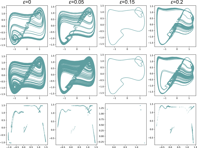
Figure 1: Lissajou plots and peak-to-peak maps for the ground-truth ($q=17$) Ikeda cubic system with system delay parameters $\tau=1.62$ and (left to right) $\varepsilon=0,0.05,0.15,0.2$. The top row contains Lissajou plots over the time interval [0,250], the middle row contains Lissajou plots over the time interval [0,1e3], and the bottom row contains peak-to-peak maps for peaks extracted from solutions over the time interval [0,2.5e3].

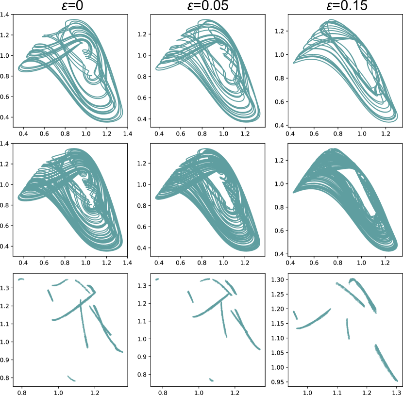
Figure 2: Lissajou plots and peak-to-peak maps for the ground-truth ($q=17$) Mackey-Glass system with system delay parameters $\tau=2$ and (left to right) $\varepsilon=0,0.05,0.15$. The top row contains Lissajou plots over the time interval [0,50], the middle row contains Lissajou plots over the time interval [0,150], and the bottom row contains peak-to-peak maps for peaks extracted from solutions over the time interval [0,2.5e3].

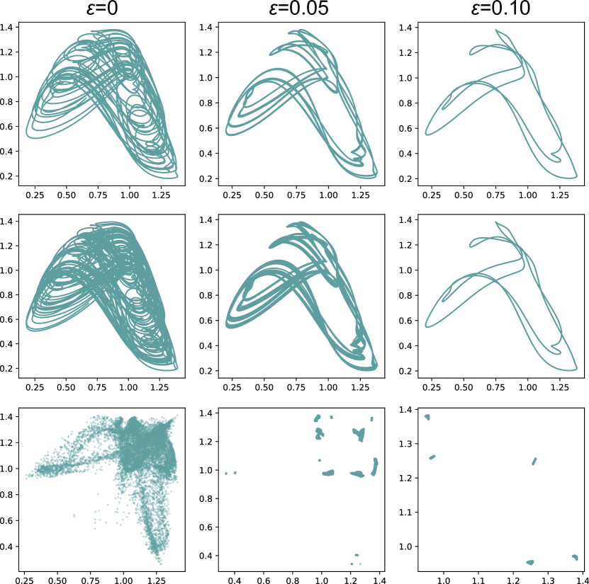
Figure 3: Lissajou plots and peak-to-peak maps for the ground-truth ($q=17$) Mackey-Glass system with system delay parameters $\tau=4$ and (left to right) $\varepsilon=0,0.05,0.1$. The top row contains Lissajou plots over the time interval [0,50], the middle row contains Lissajou plots over the time interval [0,100], and the bottom row contains peak-to-peak maps for peaks extracted from solutions over the time interval [0,2.5e3].

A striking feature that is consistent across these systems and system parameters is the apparent, often dramatic, convergence/stabilization of peak-to-peak dynamics as one increases the number of interpolating nodes, $q$, and a variety of changes in apparent system complexity for small $q$. For example, for the Ikeda system with $\varepsilon=0$ and $q<4$, the peak-to-peak dynamics are markedly different than for the ground truth system, and suggest reduced dynamic complexity. However, for $q\geq 4$ there is little perceptible difference between the approximations and the $q=17$ map (Figure 4).

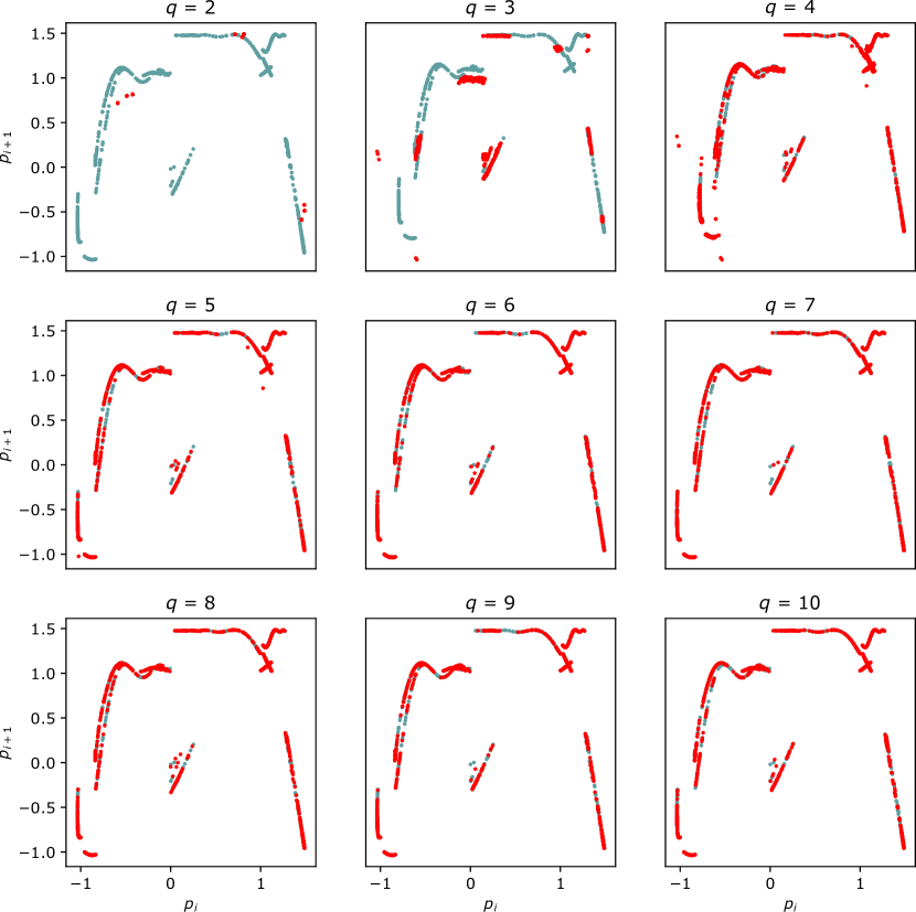
Figure 4: Peak-to-peak maps for the ground-truth ($q=17$) Ikeda system with system delay parameters $\tau=1.62$ and $\varepsilon=0$ (blue dots) compared to approximating system ($q=2,\ldots,10$, red dots). Peaks extracted from solutions over the time interval [0,2.5e3].

In contrast, the true Mackey-Glass system with $\tau=4$ and $\varepsilon=0.1$ appears to be periodic, while the approximate systems $q=3,4,5,6$ appear to be highly chaotic (Figure 5). Interestingly, the dynamics appears to have become periodic by $q=7,8,9$ but with extra peak pairs compared to the true system. These spurious peaks appear to be entirely eliminated by $q=10$, at which point there appears to be good agreement with the true system, suggesting the approximation has stabilized.

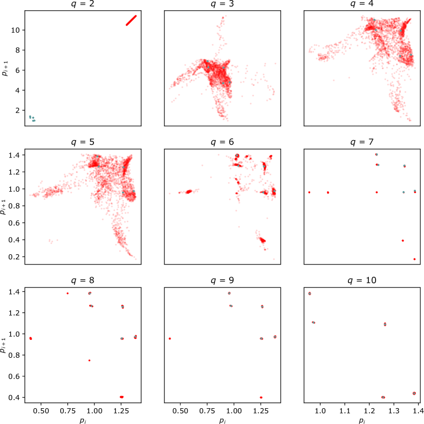
Figure 5: Peak-to-peak maps for the ground-truth ($q=17$) Mackey-Glass system with system delay parameters $\tau=4$ and $\varepsilon=0.1$ (blue dots) compared to approximating system ($q=2,\ldots,10$, red dots). Peaks extracted from solutions over the time interval [0,2.5e3].

Analogous plots for all choices of systems given in Table 1 are provided in the supplement, and showcase the significant dependence of dynamics on $q$, at least for small $q$. That said, in all cases explored here, there is eventually good agreement between the peak-to-peak maps for $q\leq 10$ (often for much smaller $q$) and the ground truth solutions.

To quantify the apparent convergence/stabilization of approximate solutions across different numbers of interpolating nodes, we constructed delay embeddings of time series samples of each trajectory, after normalizing by the standard deviation of the time series. More precisely, we constructed temporally-ordered point clouds $\{{\bm{y}_{i}}\}\subset R^{d}$ with

$$\bm{y}_{i}=[y_{i},y_{i+1},\ldots,y_{i+d-1}],$$

$y_{i}=y(i-1)/\text{std}(\{y_{i}\})$, for $i=1,\ldots,$ 1e4, and $d=3$ for the Ikeda systems and the Mackey-Glass systems with $\tau=2$ or $d=4$ for the Mackey-Glass systems with $\tau=4$. These embedding dimensions were chosen because they yielded less than 1% false nearest neighbors using the false nearest neighbor criterion [19] with thresholds $R_{\text{tol}}=10$ and $A_{\text{tol}}=2$, and so we expect are sufficiently large to unfold the underlying attractors. Thus, for each simulation a point cloud consisting of approximately 1e4 points in either $\mathbb{R}^{3}$ or $\mathbb{R}^{4}$ was constructed, ostensibly capturing a sampling of a diffeomorphic copy of the underlying attractor.

As a first, coarse comparison of dynamic behavior we estimated the correlation dimension (CD) [13] of the apparent underlying attractor of each system given in Table 1. For details see Section 7.1.1. The median and interquartile ranges of the estimated CD are given in Tables 2, 3 and 4.

We further refined the comparison of attractor structure beyond dimension using persistence homology to quantify topological structures of the attractors. In particular we computed quantified representations (persistence diagrams) of the connectivity, hole, and void structures of the delay embeddings. For details see Section 7.1.2. The median and interquartile ranges of the Wasserstein distances between $H_{0}$, $H_{1}$, and $H_{2}$ diagrams are given in Tables 2, 3 and 4.

For the Ikeda cubic system with $\tau=1.62$ and $\varepsilon=0$ the quantitative metrics reinforce the qualitative observations made using peak-to-peak maps. For instance, for the Ikeda system with $\varepsilon=0$, the apparent stabilization of the estimated correlation dimension and topological structure occurs at $q=4$ (Figure 6). The discrepancies between these structural features for $q<4$ and $q\geq 4$ is pronounced across each metric, except perhaps the Wasserstein distances between $H_{2}$ diagrams—although we note that the median Wasserstein distances for the $H_{2}$ diagrams do, in fact, fall outside the baseline interquartile ranges only for $q<4$. We expect this diminished convergence signal is due to the absence of any high-persistence $H_{2}$ classes, as can be seen in the $H_{2}$ diagrams (Figure 6 (b)). This indicates the attractors do not exhibit high-persistence void structures, which is consistent with the Lissajou plots of the ground-truth system (Figure 6) and the estimated correlation dimensions (Table 2).

The sudden stabilization of attractor structural features at a small number of interpolating nodes appears to be a general phenomenon across a range of parameters (See Tables 2, 3 and 4). However, we observe a variety of behaviors for different systems and system delay parameters as $q$ increases. For example, for the Mackey-Glass map with $\tau=4$ and $\varepsilon=0.1$ we observe notably higher correlation dimensions for $q=3,4,5,6$ than the ground truth system and higher-persistence $H_{2}$ classes, which is reflected in the Wasserstein distances between the $H_{2}$ diagrams in this range of $q$ and the ground truth diagrams being much larger than might be expected due to topological noise and finite sampling (Figure 7). The same observation holds for the Ikeda system with $\varepsilon=0.15$ and $q=3,4$. Interestingly, for $q=5$, the system appears to collapse to very nearly a periodic orbit. For both of these cases, the true system appears to be 1-dimensional topological circle (Figures 3 and 1), with stabilization occurring around $q=9$ for Mackey-Glass (Table 4) and $q=7$ for Ikeda (Table 2).

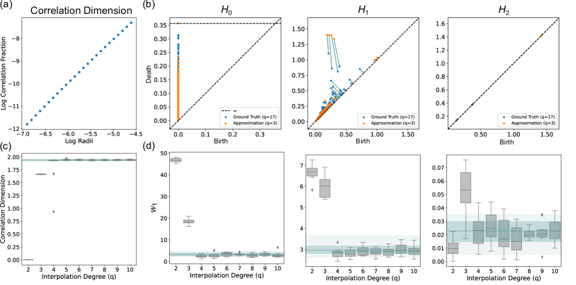
Figure 6: Quantitative metrics for the Ikeda cubic system with system delay parameters $\tau=1.62$ and $\varepsilon=0$. (a) Log of correlation fraction ($C_{i}$) against log of radii parameter ($r_{i}$) for a single sampling of the ground truth attractor ($q=17$). Example of data used to estimate the correlation dimension as the slope of the line of best fit. (b) $H_{0}$, $H_{1}$, and $H_{2}$ persistence diagrams for a single sampling of the ground truth attractor ($q=17$) and the corresponding $q=3$ approximation. The persistence pair matching which achieves the $W_{1}$ distance is shown for the $H_{1}$ diagrams. (c) Box plots of correlation dimension estimates over multiple samplings of the attractors for different numbers of approximations of interpolating nodes. Also shown is the median (solid horizontal line), interquartile range (dark shaded region), and extent (light shaded region) of the correlation dimension estimates for samplings of the ground truth attractor. (d) Box plots of 1-Wasserstein distances between $H_{0}$, $H_{1}$, and $H_{2}$ diagrams over multiple samplings of the attractors for different numbers of interpolating nodes. Also shown are the median (solid horizontal line), interquartile range (dark shaded region), and maximum extent (light shaded region) of the 1-Wasserstein distances between different samplings of the ground truth attractor.

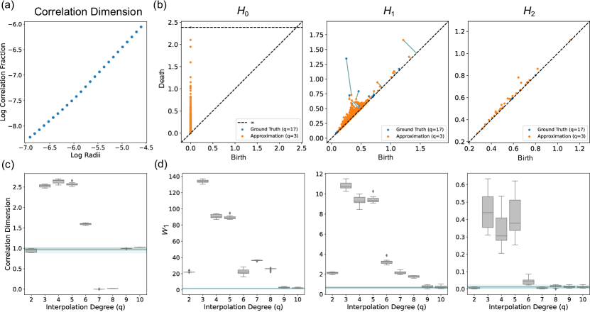
Figure 7: Quantitative metrics for the Mackey-Glass system with system delay parameters $\tau=4$ and $\varepsilon=0.1$. (a) Log of correlation fraction ($C_{i}$) against log of radii parameter ($r_{i}$) for a single sampling of the ground truth attractor ($q=17$). Example of data used to estimate the correlation dimension as the slope of the line of best fit. (b) $H_{0}$, $H_{1}$, and $H_{2}$ persistence diagrams for a single sampling of the ground truth attractor ($q=17$) and the corresponding $q=3$ approximation. The persistence pair matching which achieves the $W_{1}$ distance is shown for the $H_{1}$ diagrams. (c) Box plots of correlation dimension estimates over multiple samplings of the attractors for different numbers of approximations of interpolating nodes. Also shown is the median (solid horizontal line), interquartile range (dark shaded region), and extent (light shaded region) of the correlation dimension estimates for samplings of the ground truth attractor. (d) Box plots of 1-Wasserstein distances between $H_{0}$, $H_{1}$, and $H_{2}$ diagrams over multiple samplings of the attractors for different numbers of interpolating nodes. Also shown are the median (solid horizontal line), interquartile range (dark shaded region), and maximum extent (light shaded region) of the 1-Wasserstein distances between different samplings of the ground truth attractor.

		2	3	4	5	6	7	8	9	10	baseline
eps	metric
0	Dim.	0.00 (0.0)	1.66 (0.0)	1.93 (0.0)	1.94 (0.0)	1.94 (0.0)	1.94 (0.0)	1.94 (0.0)	1.94 (0.0)	1.95 (0.0)	1.94 (0.0)
	$H_{0}$	46.71 (1.5)	18.28 (1.3)	2.48 (0.9)	2.61 (1.1)	3.63 (1.6)	3.23 (0.4)	2.78 (1.3)	3.38 (1.0)	2.65 (0.8)	3.22 (1.3)
	$H_{1}$	6.70 (0.4)	6.02 (0.9)	2.84 (0.3)	2.78 (0.3)	2.91 (0.4)	2.88 (0.3)	2.91 (0.3)	2.96 (0.4)	2.91 (0.3)	2.96 (0.4)
	$H_{2}$	0.01 (0.0)	0.05 (0.0)	0.02 (0.0)	0.02 (0.0)	0.02 (0.0)	0.02 (0.0)	0.02 (0.0)	0.02 (0.0)	0.02 (0.0)	0.02 (0.0)
0.05	Dim.	0.02 (0.0)	1.88 (0.0)	1.94 (0.0)	1.92 (0.0)	1.94 (0.0)	1.94 (0.0)	1.94 (0.0)	1.94 (0.0)	1.94 (0.0)	1.94 (0.0)
	$H_{0}$	41.64 (15.8)	8.08 (2.4)	2.87 (0.8)	2.95 (0.9)	2.63 (1.3)	2.59 (1.0)	2.69 (0.9)	3.25 (1.1)	2.75 (0.9)	3.43 (1.5)
	$H_{1}$	5.37 (0.9)	3.04 (0.2)	2.49 (0.1)	2.53 (0.2)	2.40 (0.1)	2.43 (0.2)	2.54 (0.2)	2.42 (0.2)	2.57 (0.2)	2.51 (0.2)
	$H_{2}$	0.01 (0.0)	0.01 (0.0)	0.02 (0.0)	0.02 (0.0)	0.02 (0.0)	0.02 (0.0)	0.03 (0.0)	0.02 (0.0)	0.02 (0.0)	0.01 (0.0)
0.15	Dim.	-	1.73 (0.0)	1.21 (0.0)	0.00 (0.0)	0.98 (0.0)	1.01 (0.0)	1.02 (0.0)	1.02 (0.0)	1.01 (0.0)	1.01 (0.0)
	$H_{0}$	-	25.93 (0.6)	2.96 (0.3)	20.87 (0.3)	10.17 (0.4)	0.84 (0.1)	0.87 (0.1)	0.86 (0.2)	0.62 (0.3)	0.68 (0.2)
	$H_{1}$	-	2.45 (0.1)	0.22 (0.1)	1.04 (0.0)	0.41 (0.0)	0.04 (0.0)	0.04 (0.0)	0.05 (0.0)	0.03 (0.0)	0.03 (0.0)
	$H_{2}$	-	0.01 (0.0)	0.00 (0.0)	0.00 (0.0)	0.00 (0.0)	0.00 (0.0)	0.00 (0.0)	0.00 (0.0)	0.00 (0.0)	0.00 (0.0)
0.2	Dim.	1.00 (0.0)	-	-	1.82 (0.0)	1.74 (0.0)	1.77 (0.0)	1.79 (0.0)	1.79 (0.0)	1.79 (0.0)	1.79 (0.0)
	$H_{0}$	39.22 (1.7)	-	-	3.55 (2.0)	3.38 (0.8)	3.32 (1.9)	3.35 (1.6)	3.13 (0.8)	3.18 (1.6)	4.25 (1.8)
	$H_{1}$	4.54 (0.7)	-	-	2.80 (0.4)	2.66 (0.6)	2.71 (0.2)	2.71 (0.5)	2.54 (0.5)	2.79 (0.6)	2.80 (0.2)
	$H_{2}$	0.02 (0.0)	-	-	0.03 (0.0)	0.03 (0.0)	0.03 (0.0)	0.03 (0.0)	0.03 (0.0)	0.04 (0.0)	0.04 (0.0)

Table 2: Quantitative Comparisons of Attractors, Cubic Ikeda, $\tau=1.62$: For each choice of state-dependent delay parameter $\varepsilon$, the top rows provide median and interquartile ranges of estimated correlation dimensions (Dim.) across different numbers of interpolating nodes ($q=2,\ldots 10$) and estimates for $q=17$ in the baseline column. Rows 2,3, and 4 give median and interquartile ranges of the 1-Wasserstein distance between $H_{0}$, $H_{1}$, and $H_{2}$ persistence diagrams between the approximate systems ($q<17$) and the ground truth system ($q=17$), with baseline median and interquratile ranges measuring 1-Wasserstein distances between diaagrams corresponding to different random samplings of the ground truth ($q=17$) attractor. Missing values due to numerical instabilities for these choices of $q$.

		2	3	4	5	6	7	8	9	10	baseline
eps	metric
0	Dim.	0.02 (0.0)	1.81 (0.0)	1.94 (0.0)	2.09 (0.0)	2.09 (0.0)	2.09 (0.0)	2.08 (0.0)	2.09 (0.0)	2.08 (0.0)	2.10 (0.0)
	$H_{0}$	73.57 (1.1)	18.59 (1.2)	3.82 (1.6)	2.58 (0.6)	3.14 (0.7)	3.76 (1.3)	2.99 (0.8)	2.77 (1.3)	3.15 (0.9)	3.24 (0.9)
	$H_{1}$	9.65 (0.3)	4.42 (0.5)	3.15 (0.2)	3.00 (0.3)	2.95 (0.3)	3.00 (0.3)	3.23 (0.6)	3.25 (0.6)	2.97 (0.4)	3.10 (0.6)
	$H_{2}$	0.18 (0.1)	0.17 (0.1)	0.21 (0.1)	0.25 (0.1)	0.21 (0.0)	0.22 (0.0)	0.23 (0.1)	0.21 (0.1)	0.20 (0.1)	0.21 (0.0)
0.05	Dim.	-0.00 (0.0)	1.52 (0.0)	1.96 (0.0)	2.08 (0.0)	2.11 (0.0)	2.12 (0.0)	2.11 (0.0)	2.10 (0.0)	2.10 (0.0)	2.11 (0.0)
	$H_{0}$	64.46 (0.8)	33.29 (1.8)	4.22 (1.1)	2.38 (0.8)	2.48 (1.1)	2.44 (0.8)	2.27 (0.6)	1.99 (1.0)	2.48 (0.9)	2.14 (0.5)
	$H_{1}$	8.56 (0.3)	6.65 (0.5)	2.73 (0.3)	2.63 (0.4)	2.71 (0.2)	2.75 (0.3)	2.67 (0.4)	2.78 (0.3)	2.63 (0.3)	2.83 (0.4)
	$H_{2}$	0.10 (0.1)	0.07 (0.1)	0.11 (0.0)	0.09 (0.0)	0.11 (0.0)	0.09 (0.0)	0.10 (0.0)	0.10 (0.0)	0.09 (0.0)	0.11 (0.1)
0.15	Dim.	1.70 (0.0)	1.54 (0.0)	1.99 (0.0)	2.06 (0.0)	2.04 (0.0)	2.04 (0.0)	2.02 (0.0)	2.03 (0.0)	2.03 (0.0)	2.02 (0.0)
	$H_{0}$	12.58 (3.4)	12.59 (2.1)	2.41 (0.8)	2.25 (0.9)	2.20 (0.4)	2.05 (0.5)	2.12 (0.7)	2.02 (0.5)	2.70 (0.5)	2.49 (0.6)
	$H_{1}$	3.75 (0.4)	3.44 (0.6)	2.42 (0.1)	2.32 (0.2)	2.30 (0.3)	2.33 (0.2)	2.35 (0.4)	2.31 (0.1)	2.34 (0.3)	2.34 (0.2)
	$H_{2}$	0.03 (0.0)	0.03 (0.0)	0.03 (0.0)	0.04 (0.0)	0.03 (0.0)	0.04 (0.0)	0.04 (0.0)	0.03 (0.0)	0.03 (0.0)	0.03 (0.0)

Table 3: Quantitative Comparisons of Attractors, Mackey-Glass, $\tau=2$: For each choice of state-dependent delay parameter $\varepsilon$, the top rows provide median and interquartile ranges of estimated correlation dimensions (Dim.) across different numbers of interpolating nodes ($q=2,\ldots 10$) and estimates for $q=17$ in the baseline column. Rows 2,3, and 4 give median and interquartile ranges of the 1-Wasserstein distance between $H_{0}$, $H_{1}$, and $H_{2}$ persistence diagrams between the approximate systems ($q<17$) and the ground truth system ($q=17$), with baseline median and interquratile ranges measuring 1-Wasserstein distances between diaagrams corresponding to different random samplings of the ground truth ($q=17$) attractor.

		2	3	4	5	6	7	8	9	10	baseline
eps	metric
0	Dim.	-0.00 (0.0)	1.02 (0.0)	3.17 (0.1)	3.59 (0.3)	3.64 (0.5)	3.36 (0.3)	3.56 (0.4)	3.45 (0.2)	3.55 (0.6)	3.42 (0.4)
	$H_{0}$	173.48 (2.5)	179.31 (7.4)	15.29 (6.8)	7.03 (4.8)	5.86 (3.0)	5.38 (1.1)	5.20 (2.7)	6.43 (1.7)	6.91 (1.7)	6.26 (3.8)
	$H_{1}$	19.60 (1.1)	20.63 (1.2)	6.83 (1.7)	5.82 (0.9)	5.83 (0.6)	5.76 (0.6)	5.80 (0.8)	5.79 (0.6)	6.25 (0.8)	5.90 (0.5)
	$H_{2}$	1.62 (0.2)	1.63 (0.2)	1.48 (0.2)	1.36 (0.1)	1.36 (0.2)	1.26 (0.3)	1.38 (0.3)	1.30 (0.2)	1.28 (0.1)	1.28 (0.2)
0.05	Dim.	1.01 (0.0)	2.45 (0.1)	2.46 (0.1)	2.95 (0.1)	2.51 (0.1)	2.18 (0.0)	2.05 (0.0)	1.72 (0.1)	1.90 (0.3)	2.12 (0.0)
	$H_{0}$	59.26 (3.5)	82.25 (12.3)	90.36 (10.5)	94.19 (8.5)	40.90 (6.2)	16.58 (5.3)	7.03 (3.0)	23.98 (16.7)	9.03 (10.1)	8.46 (8.0)
	$H_{1}$	5.52 (0.5)	11.10 (1.9)	12.03 (1.9)	12.15 (1.2)	5.97 (0.6)	3.44 (0.4)	2.67 (0.8)	3.91 (1.2)	2.86 (1.2)	3.07 (1.2)
	$H_{2}$	0.03 (0.0)	0.63 (0.1)	0.73 (0.2)	0.73 (0.1)	0.21 (0.1)	0.08 (0.0)	0.07 (0.0)	0.04 (0.0)	0.06 (0.0)	0.07 (0.0)
0.1	Dim.	0.97 (0.1)	2.54 (0.1)	2.66 (0.1)	2.57 (0.0)	1.60 (0.0)	0.00 (0.0)	0.02 (0.0)	1.00 (0.0)	1.03 (0.0)	0.98 (0.1)
	$H_{0}$	21.92 (0.2)	133.94 (2.7)	90.04 (3.9)	88.88 (2.3)	21.84 (4.2)	36.35 (0.4)	26.14 (0.3)	3.15 (0.9)	2.45 (0.5)	1.71 (0.8)
	$H_{1}$	2.14 (0.1)	10.74 (0.5)	9.28 (0.5)	9.35 (0.4)	3.23 (0.2)	2.13 (0.2)	1.75 (0.2)	0.76 (0.2)	0.68 (0.2)	0.65 (0.1)
	$H_{2}$	0.00 (0.0)	0.44 (0.2)	0.31 (0.1)	0.38 (0.2)	0.04 (0.0)	0.00 (0.0)	0.02 (0.0)	0.01 (0.0)	0.01 (0.0)	0.01 (0.0)

Table 4: Quantitative Comparisons of Attractors, Mackey-Glass, $\tau=4$: For each choice of state-dependent delay parameter $\varepsilon$, the top rows provide median and interquartile ranges of estimated correlation dimensions (Dim.) across different numbers of interpolating nodes ($q=2,\ldots 10$) and estimates for $q=17$ in the baseline column. Rows 2,3, and 4 give median and interquartile ranges of the 1-Wasserstein distance between $H_{0}$, $H_{1}$, and $H_{2}$ persistence diagrams between the approximate systems ($q<17$) and the ground truth system ($q=17$), with baseline median and interquratile ranges measuring 1-Wasserstein distances between diaagrams corresponding to different random samplings of the ground truth ($q=17$) attractor.

6 Conclusions

In this work we implemented and profiled an iterative and perturbative numerical scheme for computing orbits of state dependent perturbations of delay maps. After showing local convergence of the algorithm, we also explored its more qualitative behaviors. Our empirical investigations suggest that the estimated correlation dimensions, the peak-to-peak, and Lissajou plots of the analyzed systems support low-dimensional chaotic dynamics across a range of state-dependent delays, and remind us of those infinite-dimensional systems known to support inertial manifolds. We observe also windows of the state-dependent delay parameter on which the apparent chaotic dynamics of the state-independent delay system appear to collapse to periodic orbits.

We observe apparent convergence of qualitative and quantitative features of the dynamics for relatively small numbers of interpolating nodes ($q\leq 10$) across systems and system parameters. Furthermore, we observe a rich set of behaviors for small values of $q$, in contrast to the ground truth systems. For instance, for sufficiently large $q$ the system may be periodic, behaving qualitatively like the true flow the map represents, while for smaller $q$ the map can appear to exhibit chaotic dynamics.

We believe that the above observations hold for a large class of systems similar to those under consideration in this paper; that is, when the right hand side of the DDE depends in a linear manner with respect to the instantaneous state variable $x(t)$ (even if the dependence in the delayed variable is more complex). We also believe that those observations extend to more general systems where the solution of Eq. (6), being a fixed point of a specific Picard operator, can be computed thanks to a Newton-like method. This question will be explored in a forthcoming project.

7 Methods

7.1 Quantitative Attractor Metrics

7.1.1 Correlation Dimension

In [13] it was argued that the correlation integral,

$$C(l):=\lim_{N\rightarrow\infty}\#\{(m,n)\;|\;\|{\bm{y}}_{m}-{\bm{y}}_{n}\|<l\}/N^{2},$$

grows according to a power law

$$C(l)\sim l^{\nu},$$

when ${\bm{y}}_{m}$ are points on an attractor associated with a nonlinear dissipative dynamical system sampled at fixed time increments.

It was proposed that the CD, $\nu$, serves as a measure of dynamic complexity and is related to other measures such as the Hausdorff [16] and information dimensions [10], while being more readily computable using standard linear regression, in the log-log plane, of estimates of $C(l)$ for small $l$.

For each choice of system parameters in this study and for each number of interpolating nodes, $q$, fifty simulations were performed with random initial conditions. From these, ten sets of five embedded point clouds were concatenated to very densely sample each system’s attractor. The CD of each resulting point cloud was then estimated—using standard linear regression—as the slope of the line of best fit through twenty-five data points, $(\log(C_{i}),\log(r_{i}))$, with $r_{i}$ being logarithmically spaced in the interval [1e-3, 1e-2] and

$$C_{i}=2\#\{(m,n)\;|\;1\leq m<n\leq N,\|{\bm{y}}_{m}-{\bm{y}}_{n}\|<r_{i}\}/N(N-1)$$

being the fraction of Euclidean distances between distinct points in the cloud that are less than $r_{i}$. We refer to $C_{i}$ as the correlation fraction corresponding to the radius parameter $r_{i}$.

7.1.2 Persistent Homology

In addition to CD, we computed three topological descriptors of the reconstructed attractors using persistent homology (PH). Recently PH has found widespread use across experimental sciences and in machine learning applications for its ability to extract and represent quantified shape-based features. For completeness we provide a brief description of the particular use of PH in this study. For a more complete treatment of the subject and its applications see one of the recent review articles [24, 1, 5].

PH may be regarded as a transformation mapping a finite point-cloud ${\bm{Y}}:=\{{\bm{y}}_{m}\}\subset\mathbb{R}^{d}$ to a collection of so-called persistence diagrams (PD) of the form

$$\text{dgm}_{k}({\bm{Y}})=\{(b_{i},d_{i})\;|\;b_{i}<d_{i}\in\mathbb{R}\}\cup\prod_{n=1}^{\infty}\Delta,$$

where $\Delta:=\{(x,x)\;|\;x\in\mathbb{R}\}$ is the diagonal in the plane, $k\geq 0$. Thus, each PD consists of a finite multiset of planar points above the diagonal with countably infinitely many copies of the diagonal. We refer to elements of a PD as persistence pairs.

The inclusion of copies of the diagonal allows us to define the $p$-Wasserstein distance ($p\geq 1$) between PDs:

$$W_{p}(\text{dgm}_{k}({\bm{Y}}),\text{dgm}_{k}({\bm{X}})):=\inf_{\phi}\left(\sum_{{\bm{a}}\in\text{dgm}_{k}({\bm{Y}})}\|{\bm{a}}-\phi({\bm{a}})\|^{p}\right)^{1/p},$$

where the infimum is taken over all bijections $\phi:\text{dgm}_{k}({\bm{Y}})\rightarrow\text{dgm}_{k}({\bm{Y}})$. Intuitively, $W_{p}$ measures the minimal sum of distances between matchings of persistence pairs in two diagrams among all possible pairings of those points, allowing off-diagonal pairs in one diagram to pair to diagonal points in the other. Although the sum is technically over a countably-infinite multiset, only off-diagonal pairs will contribute to the sum for a bijection which realizes the infimum, which must exist for diagrams with finitely many off-diagonal pairs.

A persistence diagram can be constructed from a finite simplicial complex $K$ by defining a filtration on it, $\emptyset=K_{0}\subseteq K_{1}\subseteq\ldots\subseteq K_{n}=K,$ thought of as a nested family of simplicial complexes. Computing dimension-$k$ simplicial homology over a field $\mathbb{K}$ on each complex produces a persistence module

$$\textbf{H}_{k}(K):=(0=H_{k}(K_{0})\xrightarrow[]{f_{k}^{0}}H_{k}(K_{1})\xrightarrow[]{f_{k}^{1}}\cdots\xrightarrow[]{f_{k}^{n-1}}H_{k}(K_{n})=H_{k}(K)),$$

comprised of vector spaces over $\mathbb{K}$ connected by linear maps

$$f_{k}^{i,j}:=f_{k}^{j-1}\circ\cdots\circ f_{k}^{i}:H_{k}(K_{i})\rightarrow H_{k}(K_{j}),$$

induced by inclusion at the level of the simplicial complexes for each $i\leq j$. $\textbf{H}_{k}(K)$ can be decomposed into a direct sum,

$$\bigoplus_{[a,b)\in\mathcal{D}_{k}}I_{[a,b)},$$

of so-called interval (persistence) modules of the form

$$I_{[a,b)}=(V_{1}\rightarrow\cdots\rightarrow V_{n}),$$

where

$$V_{i}=\begin{cases}\mathbb{K},&i\in[a,b)\\ 0,&\text{otherwise}\end{cases}$$

that are connected by maps $f^{i,j}:V_{i}\rightarrow V_{j}$ where $f^{i,j}$ is the identity map if $a\leq i\leq j<b$ and identically 0 otherwise, and the collection of intervals $\mathcal{D}_{k}$ are uniquely determined by the filtration.

Intuitively each interval $[a,b)$ in the interval-module representation encodes a $k$-dimensional homology class that is born (first appears) when moving from some $\text{K}_{i-1}$ to $\text{K}_{i}$ and which dies (becomes homologous to a class which was born earlier) when moving from $\text{K}_{j-1}$ to $\text{K}_{j}$. We refer to the value $b-a$ as the persistence or lifetime of the class corresponding to the interval $[a,b)$. Note, some classed may never die, giving rise to an unbounded interval $[a,\infty)$, but we will omit these from diagrams and calculation of $W_{p}$ between diagrams. The algebraic information in the interval modules is encoded into a persistence diagram $\text{dgm}_{k}(K)=\{(a,b)\;|\;[a,b)\in D_{k},a,b\in\mathbb{R}\}$ where the birth and death filtration values of each finite-persistence $k$-dimensional homological feature appears and later dies as a result of the filtration.

Here we adopt the commonly used Vietoris-Rips (VR) filtration to construct a filtered simplicial complex from a finite point cloud ${\bm{Y}}=\{{\bm{y}}_{m}\}$, sampled from an attractor. In particular, let $\partial_{i}$ be the $i$-th smallest distance between any two points in ${\bm{Y}}$ and define

$$\text{VR}_{i}({\bm{Y}}):=\{\sigma\subset{\bm{Y}}\;|\;\|{\bm{y}}_{i}-{\bm{y}}_{j}\|\leq\partial_{i},\text{ for all }{\bm{y}}_{i},{\bm{y}}_{j}\in\sigma\}$$

to be the simplicial complex consisting of all subsets whose diameter is less than $\partial_{i}$.

We regard this filtration as starting with $\text{VR}_{1}=\{\{{\bm{y}}_{m}\}|{\bm{y}}_{m}\in{\bm{Y}}\}$ (at $\partial_{1}=0$), consisting only of 0-dimensional simplices corresponding to the points in the cloud. Edges are added between pairs of points in order from nearest to farthest, with each higher dimensional simplex appearing at the filtration value corresponding to the diameter of the points corresponding to its vertices. In this way, we construct a nested family of complexes meant to capture the intrinsic multiscale geometry of the point cloud.

Crucial to the use of persistent homology in applications are the numerous stability results which establish—under a variety of assumptions about the data and the metrics placed on data and the diagrams—the (Lipschitz) continuity of these transformations sending data to persistence diagrams [4] [7]. Recently, general stability results for $W_{p}$, and partial results for $W_{p}$ when applied to the special case of the VR filtration used here were established [26].

For each choice of system parameters in this study and for each number of interpolating nodes, 1000 points were randomly subselected from each of ten attractor point clouds generated from ten different initial conditions. $H_{0}$, $H_{1}$, and $H_{2}$ persistence diagrams were computed from the the VR filtered simplicial complexes built on each set of 1000 points using the Ripser algorithm [2, 28]. The 1-Wasserstein distances between the diagrams derived from each approximate system ($q=2,\ldots,10$) and the ground truth system ($q=17$) were then computed. To serve as a baseline for comparison, and to account for topological noise due to finite sampling of the attractors, the 1-Wasserstein distances between ten pairs of ground truth diagrams were also computed.

References

- [1] Henry Adams and Michael Moy. Topology applied to machine learning: From global to local. Frontiers in Artificial Intelligence, 4, 2021.
- [2] Ulrich Bauer. Ripser: efficient computation of vietoris–rips persistence barcodes. Journal of Applied and Computational Topology, 5(3):391–423, Sep 2021.
- [3] Alfonso Casal, Livia Corsi, and Rafael de la Llave. Expansions in the delay of quasi-periodic solutions for state dependent delay equations. J. Phys. A, 53(23):235202, 20, 2020.
- [4] Frédéric Chazal, Vin de Silva, and Steve Oudot. Persistence stability for geometric complexes. Geometriae Dedicata, 173:193–214, 2012.
- [5] Frédéric Chazal and Bertrand Michel. An introduction to topological data analysis: Fundamental and practical aspects for data scientists. Frontiers in Artificial Intelligence, 4, 2021.
- [6] Guiling Chen, Dingshi Li, Onno van Gaans, and Sjoerd Verduyn Lunel. Stability results for nonlinear functional differential equations using fixed point methods. Indag. Math. (N.S.), 29(2):671–686, 2018.
- [7] David Cohen-Steiner, Herbert Edelsbrunner, John Harer, and Yuriy Mileyko. Lipschitz functions have lp-stable persistence. Found. Comput. Math., 10(2):127–139, 2010.
- [8] B. A. J. de Wolff, F. Scarabel, S. M. Verduyn Lunel, and O. Diekmann. Pseudospectral approximation of Hopf bifurcation for delay differential equations. SIAM J. Appl. Dyn. Syst., 20(1):333–370, 2021.
- [9] O. Diekmann and S. M. Verduyn Lunel. Twin semigroups and delay equations. J. Differential Equations, 286:332–410, 2021.
- [10] J. Doyne Farmer. Chaotic attractors of an infinite-dimensional dynamical system. Physica D: Nonlinear Phenomena, 4(3):366–393, 1982.
- [11] Joan Gimeno, Jean-Philippe Lessard, JD James, and Jiaqi Yang. Persistence of periodic orbits under state-dependent delayed perturbations: computer-assisted proofs. arXiv preprint arXiv:2111.06391, 2021.
- [12] Joan Gimeno, Jiaqi Yang, and Rafael de la Llave. Numerical computation of periodic orbits and isochrons for state-dependent delay perturbation of an ODE in the plane. SIAM J. Appl. Dyn. Syst., 20(3):1514–1543, 2021.
- [13] Peter Grassberger and Itamar Procaccia. Measuring the strangeness of strange attractors. Physica D: Nonlinear Phenomena, 9(1):189–208, 1983.
- [14] Jack K. Hale and Sjoerd M. Verduyn Lunel. Introduction to functional-differential equations, volume 99 of Applied Mathematical Sciences. Springer-Verlag, New York, 1993.
- [15] Ferenc Hartung, Tibor Krisztin, Hans-Otto Walther, and Jianhong Wu. Functional differential equations with state-dependent delays: theory and applications. In Handbook of differential equations: ordinary differential equations. Vol. III, Handb. Differ. Equ., pages 435–545. Elsevier/North-Holland, Amsterdam, 2006.
- [16] Felix Hausdorff. Dimension und äußeres maß. Mathematische Annalen, 79(1):157–179, Mar 1918.
- [17] Xiaolong He and Rafael de la Llave. Construction of quasi-periodic solutions of state-dependent delay differential equations by the parameterization method II: Analytic case. J. Differential Equations, 261(3):2068–2108, 2016.
- [18] Xiaolong He and Rafael de la Llave. Construction of quasi-periodic solutions of state-dependent delay differential equations by the parameterization method I: Finitely differentiable, hyperbolic case. J. Dynam. Differential Equations, 29(4):1503–1517, 2017.
- [19] Matthew B. Kennel, Reggie Brown, and Henry D. I. Abarbanel. Determining embedding dimension for phase-space reconstruction using a geometrical construction. Phys. Rev. A, 45:3403–3411, Mar 1992.
- [20] Bernhard Lani-Wayda and Hans-Otto Walther. A Shilnikov phenomenon due to state-dependent delay, by means of the fixed point index. J. Dynam. Differential Equations, 28(3-4):627–688, 2016.
- [21] Edward N. Lorenz. Deterministic nonperiodic flow. Journal of Atmospheric Sciences, 20(2):130 – 141, 1963.
- [22] Michael C. Mackey and Leon Glass. Oscillation and Chaos in Physiological Control Systems. Science, 197(4300):287–289, July 1977.
- [23] John C. Mason and David C. Handscomb. Chebyshev polynomials. Chapman & Hall/CRC, Boca Raton, FL, 2003.
- [24] Nina Otter, Mason A. Porter, Ulrike Tillmann, Peter Grindrod, and Heather A. Harrington. A roadmap for the computation of persistent homology. EPJ Data Science, 6(1):17, Aug 2017.
- [25] Carlo Piccardi and Sergio Rinaldi. Optimal control of chaotic systems via peak-to-peak maps. Physica D: Nonlinear Phenomena, 144(3):298–308, 2000.
- [26] Primoz Skraba and Katharine Turner. Wasserstein stability for persistence diagrams, 2021.
- [27] J. C. Sprott. A simple chaotic delay differential equation. Phys. Lett. A, 366(4-5):397–402, 2007.
- [28] Christopher Tralie, Nathaniel Saul, and Rann Bar-On. Ripser.py: A lean persistent homology library for python. Journal of Open Source Software, 3(29):925, 2018.
- [29] Hans-Otto Walther. Differentiable semiflows for differential equations with state-dependent delays. Univ. Iagel. Acta Math., (41):57–66, 2003.
- [30] Hans-Otto Walther. The solution manifold and -smoothness for differential equations with state-dependent delay. J. Differential Equations, 195(1):46–65, 2003.
- [31] Hans-Otto Walther. Local invariant manifolds for delay differential equations with state space in . Electron. J. Qual. Theory Differ. Equ., pages Paper No. 85, 29, 2016.
- [32] Hans-Otto Walther. Semiflows for differential equations with locally bounded delay on solution manifolds in the space . Topol. Methods Nonlinear Anal., 48(2):507–537, 2016.
- [33] Hans-Otto Walther. Solution manifolds which are almost graphs. J. Differential Equations, 293:226–248, 2021.
- [34] Hans-Otto Walther. A finite atlas for solution manifolds of differential systems with discrete state-dependent delays. Differential Integral Equations, 35(5-6):241–276, 2022.
- [35] Jiaqi Yang, Joan Gimeno, and Rafael de la Llave. Persistence and smooth dependence on parameters of periodic orbits in functional differential equations close to an ode or an evolutionary pde. https://arxiv.org/abs/2103.05203.
- [36] Jiaqi Yang, Joan Gimeno, and Rafael de la Llave. Parameterization method for state-dependent delay perturbation of an ordinary differential equation. SIAM J. Math. Anal., 53(4):4031–4067, 2021.