Activity Detection in Distributed Massive MIMO With Pilot-Hopping and Activity Correlation

Abstract

Many real-world scenarios for massive machine-type communication involve sensors monitoring a physical phenomenon. As a consequence, the activity pattern of these sensors will be correlated. In this letter, we study how the correlation of user activities can be exploited to improve detection performance in grant-free random access systems where the users transmit pilot-hopping sequences and the detection is performed based on the received energy. We show that we can expect considerable performance gains by adding regularizers, which take the activity correlation into account, to the non-negative least squares, which has been shown to work well for independent user activity.

I Introduction

Massive machine-type communications (mMTC) is one of the core use cases of 5G [1]. mMTC refers to scenarios where many devices are sending intermittent data. This creates a vast load on the random access protocols. Random access for mMTC has been studied in many works recently [2, 3] and especially a large focus has been on grant-free random access since the communication overhead will be smaller when there is no contention resolution [4, 5]. In grant-free random access, pilots are used to both detect the active users and estimate their channels. Since, there is a huge number of devices in the system, they cannot be assigned orthogonal pilots in each coherence interval. There are two strategies to solve this problem: the first is to assign non-orthogonal pilots [5], and the second is to assign orthogonal pilots in each coherence interval, but have pilot-hopping sequences that span multiple coherence intervals [6, 4, 7].

One important relief of random access for mMTC is that, even though there is a huge number of devices, only a small fraction of them are active at a given time since they are only active when they have information to transmit. This fact makes it justifiable to cast the activity detection problem as a compressed sensing problem and solve it with algorithms that have been proven efficient in such scenarios.

In addition to assuming sparsity, additional side-information can be used to further improve the detection performance. One such example is temporal correlation of the user activity: a user is probably active in many consecutive time slots since it is active until it has transmitted all the data [8, 9]. Another type of side-information that can be exploited is correlation of the channel between the active user and the base station. This channel can be spatially correlated [10, 11] or both spatially and temporally correlated [12]. Such side-information is used to improve methods which jointly detect the active users and estimate their channels.

If the activity of the devices is governed by a physical phenomenon, we can presume that the activity of devices monitoring the same phenomenon is correlated. The previously mentioned grant-free random access algorithms [8, 9, 10, 11, 12] and protocols exploit side-information. However, using correlated user activity as side-information has been somewhat neglected for grant-free random access. One work that considers correlated user activity is [13], which considers an unsourced random access framework. In that work, the devices can either transmit standard messages, or alarm messages. The alarm messages depend on a physical phenomenon and all devices will transmit the same message in the case of an alarm. Recently, [14] considered correlated user activities in a grant-based random access setting. They found the preamble (pilot) selection distribution that minimizes preamble collisions given a correlated activity distribution.

In this paper, we generalize the transmission model proposed in [4, 6] and implemented in [7] where the devices transmit pilot-hopping sequences in order to aid in activity detection and channel estimation, see Fig. 1. A single-cell massive multiple-input-multiple-output (MIMO) system where the user activities are independent was studied in [4], while in this paper, we consider a distributed massive MIMO system with correlated user activities. The technical challenge is to formalize a detection problem that can adequately capture the activity correlation. We address this issue by solving a regularized non-negative least squares (NNLS) problem, where the regularizer takes the activity correlation into account. To the best our knowledge, this is the first work to consider correlated user activities in grant-free random access.

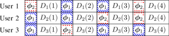
Figure 1: Three users transmitting pilot-hopping sequences of length four using two pilots, $\bm{\phi}_{1}$ and $\bm{\phi}_{2}$. Additionally, in coherence interval $t$ the user $k$ also transmits uplink data $D_{k}(t)$.

II Distributed Massive MIMO System Model

We consider a distributed MIMO system where $L$ base stations are equipped with $M$ antennas each and collectively serve $K$ single-antenna users. Note that when $L=1$, this is the standard co-located single-cell massive MIMO system model. Not all of these users are active. The activity is modeled as random but there might be correlation between users. We assume a block fading model; the channel is assumed to be time invariant and frequency flat in each coherence interval.

We study a grant-free access transmission model where each communication round spans $T$ coherence intervals. In each coherence interval there is a pilot phase, which is $\tau_{\text{p}}$ symbols long, such that there are $\tau_{\text{p}}$ orthogonal pilots, and a data phase, which spans the rest of the coherence interval. The users are assigned a unique pilot-hopping sequence wherein each of the $T$ coherence intervals one of the $\tau_{\text{p}}$ orthogonal pilots is chosen, see Fig. 1. While the pilots might collide in individual coherence intervals, the pilot collisions get averaged over the whole pilot-hopping sequence and data can still be reliably transmitted [6]. Hence, with highly frequency-selective channels, where $\tau_{\text{p}}$ will be small due to a limited coherence bandwidth, more collisions will occur per coherence block.

At the pilot phase of coherence interval $t$, the base stations collectively receive the $ML\times\tau_{\text{p}}$ signal

$$\bm{Y}^{t} =\sum_{k=1}^{K}\sum_{j=1}^{\tau_{\text{p}}}\alpha_{k}S_{j,k}^{t}\sqrt{\tau_{\text{p}}p_{k}}\bm{g}_{k}^{t}\bm{\phi}_{j}^{\mathsf{H}}+\bm{N}^{t},\;t=1,\dots,T$$ (1)

$$\text{where}\qquad\qquad\alpha_{k}=\begin{cases}1,&\text{if user }k\text{ is active,}\\ 0,&\text{otherwise,}\end{cases}$$ (2)

$$S_{j,k}^{t} =\begin{cases}1&\text{ if user }k\text{ sends pilot }j\text{ at pilot phase }t\text{,}\\ 0&\text{ otherwise,}\end{cases}$$ (3)

$p_{k}$ is the transmit power of user $k$, $\bm{g}_{k}^{t}\in\mathbb{C}^{ML}$ is the collective channel between user $k$ and the base stations in coherence interval $t$, and $\bm{\phi}_{j}\in\mathbb{C}^{\tau_{\text{p}}}$ is the $j$:th pilot consisting of $\tau_{\text{p}}$ symbols. The pilots are mutually orthogonal, $\bm{\phi}_{i}^{\mathsf{H}}\bm{\phi}_{j}=0,i\neq j$, and have unit norm, $\left\lVert\bm{\phi}_{i}\right\rVert=1$. Finally, $\bm{N}^{t}\in\mathbb{C}^{ML\times\tau_{\text{p}}}$ is noise with i.i.d. $\mathcal{CN}\left(0,\sigma^{2}\right)$ elements. The received signal in (1) can be viewed as blocks of received signals from each base station,

$$\bm{Y}^{t}=\begin{bmatrix}(\bm{Y}^{t}_{1})^{\mkern-1.5mu\mathsf{T}}&\dots&(\bm{Y}^{t}_{l})^{\mkern-1.5mu\mathsf{T}}&\dots&(\bm{Y}^{t}_{L})^{\mkern-1.5mu\mathsf{T}}\end{bmatrix}^{\mkern-1.5mu\mathsf{T}},$$ (4)

where $\bm{Y}_{l}^{t}\in\mathbb{C}^{M\times\tau_{\text{p}}}$ is the received signal at base station $l$ at the pilot phase of coherence interval $t$. The model assumes that the users are synchronized in the sense that all the active users start their pilot-hopping sequence at the same coherence interval. Hence, the same users are active during the $T$ coherence intervals in (1). If new users want to access the network, they would need to wait until the next pilot-hopping sequence starts.

II-A Asymptotic Energy System Model

In each coherence interval, an estimate of the received signal energy over each pilot is computed as

$$E_{i,t}=\frac{(\bm{Y}^{t}\bm{\phi}_{i})^{\mathsf{H}}(\bm{Y}^{t}\bm{\phi}_{i})}{ML}-\sigma^{2}=\frac{\left\lVert\bm{Y}^{t}\bm{\phi}_{i}\right\rVert^{2}}{ML}-\sigma^{2},$$ (5)

which is a sufficient statistic for the user activity. These energy estimates are used to detect the active users. Assuming that the channels have the asymptotic channel hardening property, i.e.,

$$\frac{\left\lVert\bm{g}_{k}^{t}\right\rVert^{2}}{ML}\to\beta_{k},\quad\text{ as }\quad ML\to\infty,$$ (6)

where $\beta_{k}$ is the large-scale fading coefficient, and asymptotic favorable propagation property, i.e.,

$$\frac{(\bm{g}_{k}^{t})^{\mathsf{H}}(\bm{g}_{k^{\prime}}^{t})}{ML}\to 0,\quad\text{ as }\quad ML\to\infty,k\neq{k^{\prime}},$$ (7)

we see that as $ML\to\infty$,

$$E_{i,t}=\frac{\left\lVert\bm{Y}^{t}\bm{\phi}_{i}\right\rVert^{2}}{ML}-\sigma^{2}\rightarrow\sum_{k=1}^{K}\alpha_{k}S_{i,k}^{t}\tau_{\text{p}}p_{k}\beta_{k}.$$ (8)

Channel hardening and favorable propagation are common in many propagation scenarios in massive MIMO and are fulfilled for e.g. Rayleigh fading [15, Ch. 7] [16, Ch. 2] and uniform random line-of-sight channels [15, Ch. 7]. In practice, the total number of antennas $ML$ will be finite and (8) can then be interpreted as an approximation. For the co-located case ($L~{}=~{}1$) with i.i.d. Rayleigh fading, the approximations are normally tight at around $M=50$ antennas since the variance of (6) and (7) scale with $\frac{1}{M}$ [16, Sec. 2.5].

We introduce the vector notation

$$\bm{\alpha}=\left[\alpha_{1},\dots,\alpha_{K}\right]^{\mkern-1.5mu\mathsf{T}},$$ (9)

$$\text{and }\bm{y}=\left[E_{1,1},\dots,E_{\tau_{\text{p}},1},\dots,E_{i,t},\dots E_{1,T},\dots,E_{\tau_{\text{p}},T}\right]^{\mkern-1.5mu\mathsf{T}}.$$ (10)

Further, we introduce the $\tau_{\text{p}}T~{}\times~{}K$ matrix,

$$\bm{A}=\begin{pmatrix}S_{1,1}^{1}\tau_{\text{p}}p_{1}\beta_{1}&&\cdots&&S_{1,K}^{1}\tau_{\text{p}}p_{K}\beta_{K}\\ \vdots&&\ddots&&\vdots\\ S_{\tau_{\text{p}},1}^{1}\tau_{\text{p}}p_{1}\beta_{1}&&\cdots&&S_{\tau_{\text{p}},K}^{1}\tau_{\text{p}}p_{K}\beta_{K}\\ &\ddots&&&\\ \vdots&&S_{i,k}^{t}\tau_{\text{p}}p_{k}\beta_{k}&&\vdots\\ &&&\ddots&\\ S_{1,1}^{T}\tau_{\text{p}}p_{1}\beta_{1}&&\cdots&&S_{1,K}^{T}\tau_{\text{p}}p_{K}\beta_{K}\\ \vdots&&\ddots&&\vdots\\ S_{\tau_{\text{p}},1}^{T}\tau_{\text{p}}p_{1}\beta_{1}&&\cdots&&S_{\tau_{\text{p}},K}^{T}\tau_{\text{p}}p_{K}\beta_{K}\end{pmatrix}.$$ (11)

Note that with $\tau_{\text{p}}$ pilots and $T$ coherence intervals, there are $(\tau_{\text{p}})^{T}$ unique pilot-hopping sequences. Therefore, in order for each user to have unique sequences we require $K\leq(\tau_{\text{p}})^{T}$. However, since we assume that there is a massive number of users, the product of the number of pilots and the sequence length is most likely smaller than the number of users: $\tau_{\text{p}}T~{}\leq~{}K$. Hence, the matrix $\bm{A}$ is wide. Now, we can express the limit in (8) using this notation:

$$\bm{y}\to\bm{A}\bm{\alpha}\quad\text{ as }\quad ML\to\infty.$$ (12)

With a finite number of antennas, (12) will only hold approximately. We consider the asymptotic system model to be

$$\bm{y}=\bm{A}\bm{\alpha}+\bm{n},$$ (13)

where $\bm{n}$ is the zero mean noise that is generally not Gaussian.

III User Activity Detection

We aim to detect the active users using the the received energies based on the model in (13).

III-A Independent User Activity

First, we will treat the case where the user activities are independent. Although there are fewer measurements ($\tau_{\text{p}}T$) than the number of users ($K$), we know that only a few of them are active. Hence, it is pertinent to view the active user detection problem as a compressed sensing problem. Minimizing the noise given that the $\alpha_{k}$:s are 0/1-variables gives a combinatorial problem,

$$\operatorname*{argmin}_{\bm{\alpha}\in\left\{0,1\right\}^{K}}\left\lVert\bm{A}\bm{\alpha}-\bm{y}\right\rVert^{2},$$ (14)

which is computationally costly to solve through an exhaustive search. Therefore, the problem is relaxed and we allow $\bm{\alpha}$ to take any non-negative value. The relaxed problem becomes the NNLS

$$\operatorname*{argmin}_{\bm{\alpha}\geq\bm{0}}\left\lVert\bm{A}\bm{\alpha}-\bm{y}\right\rVert^{2}.$$ (15)

After solving (15) using any convex solver, each element is thresholded to detect the active users. If $\bm{A}$ in (11) is properly normalized, it has the so-called self-regularizing property [17, Condition 1]. To show this, first note that each column of $\bm{A}$ contains exactly $T$ non-zero entries, corresponding to the pilot-hopping sequence for each user. Suppose we normalize $\bm{A}$ such that the norm of all its columns are equal. This can be achieved by forcing the received signal-to-noise ratios (SNR) for each user to be equal, i.e., the transmit power of each user should be inversely proportional to the large-scale fading coefficient, i.e., statistical channel inversion [16]: $p_{k}=\frac{p\beta_{\text{min}}}{\beta_{k}}$, where $p\tau_{\text{p}}$ is the maximum allowed transmit power per pilot and $\beta_{\text{min}}=\min_{k}\beta_{k}$. Then, take $\bm{X}=\frac{\bm{A}}{\sqrt{\tau_{\text{p}}}p\beta_{\text{min}}}$, $\bm{w}=\left[1,1,...,1\right]^{\mkern-1.5mu\mathsf{T}}$ in the definition of [17, Condition 1], and verify that the condition is satisfied.

Generally, NNLS problems with a self-regularizing measurement matrix yield sparse solutions, even without introducing an explicit sparsity-enforcing regularizer, if the noise distribution is sub-Gaussian [17, Thm. 1]; see also [18, 19, 20]. In the present context, with Rayleigh fading channels, the noise $\bm{n}$ is not sub-Gaussian as it contains products of Gaussian random variables. Therefore, [17, Thm. 1] does not strictly apply. Yet, we take the self-regularizing property of $\bm{A}$ as an explanation for why our method works and specifically yields sparse solutions in our numerical experiments.

The NNLS approach, based on measurements of signal energies as in (13), and formulation of the activity detection problem as an NNLS problem, was originally proposed in [4]; therein, however, only the single-cell case ($L=1$) was studied.

III-B Correlated User Activity

In this section, we propose an algorithm for activity detection with user activity correlation. To exploit the activity correlation in the detection, the correlation needs to be known a priori or estimated to some extent. For example, the activity correlation can be estimated based on past successful transmissions. The correlation can for example arise because the devices are monitoring the same type of event or because the devices are in the same geographical area.

Our proposed approach is to add a regularizer, $R(\bm{\alpha})$, to the NNLS in (15) to obtain

$$\min_{\bm{\alpha}\geq\bm{0}}\left\lVert\bm{A}\bm{\alpha}-\bm{y}\right\rVert^{2}+R(\bm{\alpha}).$$ (16)

We consider two different regularizers.

If $\bm{\alpha}$ is group sparse, i.e., only a few pre-determined groups of users are active, an approach from compressed sensing is to use the $\ell_{1}/\ell_{2}$-regularizer [21]

$$R(\bm{\alpha}) =\lambda\sum_{j=1}^{G}c_{j}\left\lVert\bm{\alpha}_{\mathcal{G}_{j}}\right\rVert_{2},$$ (17)

where $G$ is the number of groups, $\mathcal{G}_{j}$ is the $j$:th group, $\bm{\alpha}_{\mathcal{G}_{j}}$ denotes the sub-vector of $\bm{\alpha}$ where $\mathcal{G}_{j}$ contains the selected components, $c_{j}$ is the weight associated with the $j$:th group, and $\lambda$ is the regularization parameter which decides how much weight should be put on the regularization. If the groups are non-overlapping, this minimization problem is the group least absolute shrinkage and selection operator (LASSO) problem (with an additional non-negativity constraint) [21, Ch. 6].

If a user is more prone to be active if its neighbors are active, a suitable regularizer is

$$R(\bm{\alpha}) =\lambda\sum_{k=1}^{K}c_{k}\sqrt{\sum_{j\in\mathcal{N}(k)}\left|\alpha_{k}-\alpha_{j}\right|^{2}},$$ (18)

where $\mathcal{N}(k)$ are the neighbors of user $k$ in some correlation sense, $\bm{\alpha}_{\mathcal{N}(k)}$ denotes the sub-vector of $\bm{\alpha}$ where $\mathcal{N}(k)$ contains the selected components, $c_{k}$ is the weight associated with the $k$:th user, and $\lambda$ is the regularization parameter. This regularizer can be interpreted as the $\ell_{1}/\ell_{2}$-regularizer on the difference between users and their neighbors. The regularizer will enforce that only a few users’ activities differs from their neighbors’. This regularizer is a generalization of the isotropic two-dimensional total variation denoising used for, e.g., images, where the neighbor set contains only the directly adjacent pixels [22]. The particular choices of groups and neighbor sets will depend on the application. Here, we used an approach where all users in a group are treated equally, and equally contribute to the overall objective function. Another approach is to weigh the regularization such that user pairs with higher correlation have a higher impact.

When the activity is correlated it might not be vital exactly which users are active, but instead a detection of e.g., the monitored event is more important. Therefore, performance evaluation needs to be handled with care. In the case where the correlation comes from location based information, i.e., when users are activated by nearby events, we suggest evaluating how well different algorithms perform at detecting the position of the events. Consider $E$ events occurring at positions $\bm{e}_{i}\in\mathbb{R}^{2}$, $i=1,\dots,E$. After detecting the active users (by thresholding the results from the regularized NNLS), their positions are clustered into $E$ clusters. Note that, here it is assumed that we know the number of events through a genie but nothing prevents the estimation of the number of events. After clustering, we obtain estimates of the event positions $\hat{\bm{e}}_{j},j=1,\dots,E$. Next, we find the pairings, $\mathcal{P}=\{(i,j)\}$, such that

$$\frac{1}{E}\sum_{(i,j)\in\mathcal{P}}\left\lVert\bm{e}_{i}-\hat{\bm{e}}_{j}\right\rVert^{2}$$ (19)

is minimized. This gives the squared distance between the true and detected events.

IV Numerical simulations

In this section we study a specific simulation scenario where a set of user terminals monitor the occurrence of some event. The scenario is chosen to illustrate the potential and expected gain that is obtained by including the knowledge of user activity correlation. We simulate a scenario with $L=4$ base stations, each with $M=32$ antennas. The simulation scenario resembles an industrial Internet-of-things setting [23].

The “world” is a 2-dimensional plane, $[0,1]\times[0,1]$. There are $K=1296$ users placed on a $36\times 36$ square grid. The base stations are placed at the center of each edge, i.e., at positions $(0,0.5)$, $(1,0.5)$, $(0.5,0)$ and $(0.5,1)$. Within the plane, $E=3$ events occur uniformly at random. User $k$ at position $\bm{x}_{k}$ is activated by event $i$ at position $\bm{e}_{i}$ with probability $p_{k,i}=\exp\left(\frac{-\left\lVert\bm{x}_{k}-\bm{e}_{i}\right\rVert^{2}}{2\sigma_{e}^{2}}\right)$, where $\sigma_{e}^{2}=0.001$ is chosen such that, on average, one event approximately activates $7.5$ users.

There are $\tau_{\text{p}}=10$ orthogonal pilots and the pilot-hopping sequences span $T=10$ coherence intervals. The users’ pilot-hopping sequences are chosen uniformly at random from all the possible $(\tau_{\text{p}})^{T}$ sequences. The channels are modeled as i.i.d. Rayleigh fading; the channel between user $k$ and the $l$:th base station is $\bm{g}_{k}^{l}\sim\mathcal{CN}\left(\bm{0},\beta_{k}^{l}\bm{I}\right)$, where $\beta_{k}^{l}$ is the large-scale fading to the $l$:th base station and $\beta_{k}=\frac{1}{L}\sum_{l=1}^{L}\beta_{k}^{l}$. The large-scale fading depends on the distance to each base station: $\beta_{k}^{l}=\gamma(d_{k}^{l})^{-3.67}$, where $d_{k}^{l}$ is the distance between user $k$ and base station $l$, $3.76$ is the path-loss exponent, and $\gamma$ is a constant. The users perform statistical channel inversion power control as described in Section III-A. The SNR is defined as $\mathsf{SNR}=\frac{p\beta_{\text{min}}}{\sigma^{2}}$. In the simulation we have chosen the constant $\gamma$ such that $\mathsf{SNR}=10$ dB.

For the total-variation-inspired (TV) regularizer, the neighbor set of user $k$ is chosen as

$$\mathcal{N}(k)=\{i:\left\lVert\bm{x}_{k}-\bm{x}_{i}\right\rVert<r\},$$ (20)

where $r=0.05$ is chosen such that, when the $k$:th user is not on the edge of the grid, there are $9$ users in the set including the $k$:th user itself. For the group-LASSO-inspired (GLASSO) regularizer, the groups are chosen to be the $K$ different neighbor sets, i.e., $G=K$ and $\mathcal{G}_{k}=\mathcal{N}(k)$. Further, all users and groups have the same (unit) weight, $c_{k}=1$, for both the TV and GLASSO regularizers. All three optimization problems (NNLS, TV and GLASSO) are solved with the MOSEK [24] solver in CVXPY [25].

The probability of missed detection, $p_{\text{m}}$, and the probability of false alarm, $p_{\text{fa}}$, are defined as

$$p_{\text{m}} =\frac{\text{\# undetected active users}}{\text{\# active users}},\quad\text{and}$$ (21)

$$p_{\text{fa}} =\frac{\text{\# detected inactive users}}{\text{\# inactive users}}.$$ (22)

Fig. 2 shows the receiver operating characteristic (ROC) curves for the different methods. Different false alarm and miss detection probabilities can be achieved by choosing different thresholds. We see that both the proposed methods, TV and GLASSO, perform better, i.e., at a given false alarm probability, the miss detection probability is lower, than for NNLS when the appropriate regularization parameter, $\lambda$, is chosen. We note that in this case, with these regularization parameters, TV with $\lambda=0.06$ performs best. However, the best regularizer (and regularization parameter) will depend on application and specifically how the user activities are correlated. We conjecture that TV performs better when the activity correlation comes from the device location, as indicated by the simulations, and that GLASSO is better suited when the activity correlation is such that devices activate in predetermined groups.

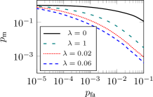
(a) TV

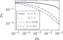
(b) GLASSO

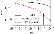
(c) Comparison

Figure 2: ROC comparison of the proposed regularizers with different regularization parameters, $\lambda$. Note that, $\lambda=0$ corresponds to NNLS for both the regularizers.

As we have seen, the proposed detection algorithms are better at detecting active users than the baseline NNLS. We also report the root-mean-square distance (RMSD) in Fig. 3, obtained by the process described in Section III-B. After detecting the active users, their positions are clustered into $E=3$ clusters by the K-means algorithm [26, Ch. 5]. In case of no detected users, we place all events in the center of the plane. From the figure, we see that taking the activity correlation into account gives more accurate event position estimates than NNLS, and we can deduce that the optimal (in terms of RMSD) threshold is somewhere between 0.4 and 0.7. In practice the threshold can be tested empirically and set based on application requirements.

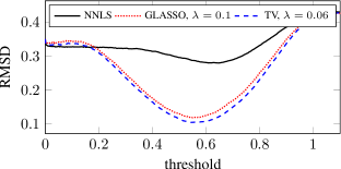
Figure 3: After the active users are detected, their positions are clustered into $E=3$ clusters and the RMSD between the cluster centers and the true event positions is reported.

We have also performed simulations with fewer antennas (not pictured due to space constraints) and although the approximation in (13) is worse, the conclusions follow the ones presented here; exploiting the activity correlation will give better performance.

V Conclusions

We studied a user activity detection problem for mMTC users in distributed massive MIMO systems. The users transmit pilot-hopping sequences and the base stations use the received energy to detect the active users. We introduced user activity correlation where we modeled users that monitor physical phenomena and hence will activate based on their occurrence. Our proposed method is to add a regularization term to the NNLS. We studied two different regularizers inspired by total variance denoising and group LASSO. By simulating a realistic system, we showed that introducing regularizers that exploit the correlation greatly improves the performance of the user activity detection, both in terms of detecting the active users and estimating the position of the event that triggered the activation of the users. Which regularizer that is best will depend on the individual problem and model.

References

- [1] IMT Vision – Framework and overall objectives of the future development of IMT for 2020 and beyond, ITU-R Std. M.2083-0, 2015.
- [2] C. Bockelmann et al., “Towards massive connectivity support for scalable mMTC communications in 5G networks,” IEEE Access, vol. 6, pp. 28 969–28 992, 2018.
- [3] X. Chen, D. W. K. Ng, W. Yu, E. G. Larsson, N. Al-Dhahir, and R. Schober, “Massive access for 5G and beyond,” IEEE Journal on Selected Areas in Communications, vol. 39, no. 3, pp. 615–637, 2021.
- [4] E. Becirovic, E. Björnson, and E. G. Larsson, “Detection of pilot-hopping sequences for grant-free random access in massive MIMO systems,” in IEEE ICASSP 2019, 2019, pp. 8380–8384.
- [5] L. Liu, E. G. Larsson, W. Yu, P. Popovski, Č. Stefanović, and E. de Carvalho, “Sparse signal processing for grant-free massive connectivity: A future paradigm for random access protocols in the internet of things,” IEEE Signal Processing Magazine, vol. 35, no. 5, pp. 88–99, 2018.
- [6] E. de Carvalho, E. Björnson, J. H. Sørensen, E. G. Larsson, and P. Popovski, “Random pilot and data access in massive MIMO for machine-type communications,” IEEE Transactions on Wireless Communications, vol. 16, no. 12, pp. 7703–7717, Dec 2017.
- [7] N. M. Sarband, E. Becirovic, M. Krysander, E. G. Larsson, and O. Gustafsson, “Massive machine-type communication pilot-hopping sequence detection architectures based on non-negative least squares for grant-free random access,” IEEE Open Journal of Circuits and Systems, vol. 2, pp. 253–264, 2021.
- [8] W. Zhu, M. Tao, and Y. Guan, “Joint user activity detection and channel estimation for temporal-correlated massive access,” in IEEE ICC 2021, 2021, pp. 1–6.
- [9] Q. Wang, L. Liu, S. Zhang, and F. C. M. Lau, “Exploiting temporal side information in massive IoT connectivity,” 2022, arxiv:2201.01485.
- [10] H. Djelouat, L. Marata, M. Leinonen, H. Alves, and M. Juntti, “User activity detection and channel estimation of spatially correlated channels via AMP in massive MTC,” in 2021 55th Asilomar Conference on Signals, Systems, and Computers, 2021, pp. 1200–1204.
- [11] H. Djelouat, M. Leinonen, and M. Juntti, “Spatial correlation aware compressed sensing for user activity detection and channel estimation in massive MTC,” IEEE Transactions on Wireless Communications, pp. 1–1, 2022.
- [12] Y. Cheng, L. Liu, and L. Ping, “Orthogonal AMP for massive access in channels with spatial and temporal correlations,” IEEE Journal on Selected Areas in Communications, vol. 39, no. 3, pp. 726–740, 2021.
- [13] K. Stern, A. E. Kalør, B. Soret, and P. Popovski, “Massive random access with common alarm messages,” in 2019 IEEE International Symposium on Information Theory (ISIT), 2019, pp. 1–5.
- [14] W. Liu, Y. Cui, F. Yang, L. Ding, and J. Sun, “Joint optimization of preamble selection and access barring for random access in MTC with general device activities,” IEEE Transactions on Communications, vol. 70, no. 6, pp. 3930–3946, 2022.
- [15] T. L. Marzetta, E. G. Larsson, H. Yang, and H. Q. Ngo, Fundamentals of Massive MIMO. Cambridge University Press, 2016.
- [16] E. Björnson, J. Hoydis, and L. Sanguinetti, “Massive MIMO networks: Spectral, energy, and hardware efficiency,” Foundations and Trends® in Signal Processing, vol. 11, no. 3-4, pp. 154–655, 2017.
- [17] M. Slawski and M. Hein, “Non-negative least squares for high-dimensional linear models: Consistency and sparse recovery without regularization,” Electron. J. Statist., vol. 7, pp. 3004–3056, 2013.
- [18] A. M. Bruckstein, M. Elad, and M. Zibulevsky, “On the uniqueness of nonnegative sparse solutions to underdetermined systems of equations,” IEEE Transactions on Information Theory, vol. 54, no. 11, pp. 4813–4820, Nov 2008.
- [19] R. Kueng and P. Jung, “Robust nonnegative sparse recovery and the nullspace property of 0/1 measurements,” IEEE Transactions on Information Theory, vol. 64, no. 2, pp. 689–703, Feb 2018.
- [20] S. Foucart and D. Koslicki, “Sparse recovery by means of nonnegative least squares,” IEEE Signal Processing Letters, vol. 21, no. 4, pp. 498–502, April 2014.
- [21] I. Rish and G. Y. Grabarnik, Sparse Modeling: Theory, Algorithms, and Applications. CRC Press, 2014.
- [22] L. Condat, “Discrete total variation: New definition and minimization,” SIAM Journal on Imaging Sciences, vol. 10, no. 3, pp. 1258–1290, 2017.
- [23] L. D. Xu, W. He, and S. Li, “Internet of things in industries: A survey,” IEEE Transactions on Industrial Informatics, vol. 10, no. 4, pp. 2233–2243, 2014.
- [24] MOSEK ApS, MOSEK Optimizer API for Python. Version 9.3., 2022. [Online]. Available: https://docs.mosek.com/9.3/pythonapi/index.html
- [25] S. Diamond and S. Boyd, “CVXPY: A Python-embedded modeling language for convex optimization,” Journal of Machine Learning Research, vol. 17, no. 83, pp. 1–5, 2016.
- [26] J. Han, M. Kamber, and J. Pei, Data Mining Concepts and Techniques, 3rd ed. Elsevier, 2012.