2022
[1,2,3]\fnmDavid \surRügamer
1]\orgdivDepartment of Statistics, \orgnameLMU Munich, \orgaddress\cityMunich, \countryGermany
2]\orgdivDepartment of Statistics, \orgnameTU Dortmund, \orgaddress\cityDortmund, \countryGermany
3]\orgdivMunich Center for Machine Learning, \orgaddress\cityMunich, \countryGermany
4]\orgdivInstitute for Statistics and Mathematics, \orgnameWU Vienna, \orgaddress\cityVienna, \countryAustria
Mixture of Experts Distributional Regression: Implementation Using Robust Estimation with Adaptive First-order Methods
Abstract
In this work, we propose an efficient implementation of mixtures of experts distributional regression models which exploits robust estimation by using stochastic first-order optimization techniques with adaptive learning rate schedulers. We take advantage of the flexibility and scalability of neural network software and implement the proposed framework in mixdistreg, an R software package that allows for the definition of mixtures of many different families, estimation in high-dimensional and large sample size settings and robust optimization based on TensorFlow. Numerical experiments with simulated and real-world data applications show that optimization is as reliable as estimation via classical approaches in many different settings and that results may be obtained for complicated scenarios where classical approaches consistently fail.
keywords:
Mixture Models, Deep Learning, Structured Additive Regression, Neural Networks1 Introduction
Mixture models are a common choice to model the joint distribution of several sub-populations or sub-classes on the basis of data from the pooled population where the sub-class memberships are not observed (for an introduction see McLachlan and Peel, 2004). Each sub-class is assumed to follow a parametric probability distribution such that the pooled observations are from a mixture of these distributions. Many applications of mixture models aim at estimating the distributions of the latent sub-classes and identifying sub-class memberships of the observations (McLachlan et al, 2019). Mixture models have also been used in machine learning, e.g., for clustering (Viroli and McLachlan, 2019), to build generative models for images (Van den Oord and Schrauwen, 2014) or as a hybrid approach for unsupervised outlier detection (Zong et al, 2018).
Different kinds of mixture models are used depending on the available data structure and the parametric model which is assumed for each sub-population or sub-class. In the following, we assume a supervised learning task and that regression models are used to model the sub-populations. This leads to mixture regression models which define a mixture of (conditional) models for the outcome of interest, where the mixture components are still unknown and thus considered latent variables. This model class is also referred to as mixtures of experts (Gormley and Frühwirth-Schnatter, 2019). Mixtures of experts allow for the inclusion of covariates when modeling the mixture components as well as for the mixture weights. In the following, we consider a mixture of experts model where the regression models do not only include the mean parameter but also other distributional parameters that may depend on the covariates or features. In addition, we assume that the sub-population sizes vary with covariates (or features). This leads to the class of mixture of experts distributional regression models.
1.1 Mixture Models and Their Estimation
As for classical statistical regression models, the goal of mixtures of regressions or mixture regression models is to describe the conditional distribution of a response (or outcome), conditional on a set of covariates (or features). Mixtures of regressions have been first introduced by Quandt (1958) under the term switching regimes where only two-component mixtures of linear regression models were considered, i.e., the number of sub-classes was fixed to two. This was extended to general mixtures of linear regression models by DeSarbo and Cron (1988) who referred to this approach as a model-based version of clusterwise regression (Späth, 1979). The extension to mixtures of generalized linear regression models was proposed in Wedel and DeSarbo (1995). Aiming for a setting beyond mean regression (Kneib, 2013), a distributional regression setting can be used such as generalized additive models for location, scale and shape (GAMLSS; Rigby and Stasinopoulos 2005) which also allow for non-linear smooth relationships between covariates and the distributional parameter of interest (Stasinopoulos et al, 2018).
Mixture models can be estimated using various techniques, with the expectation-maximization (EM) algorithm based on the maximum-likelihood principle being the most prominent one. Other approaches include Bayesian methods such as MCMC algorithms with data augmentation (Diebolt and Robert, 1994). An alternative way of model specification and estimation was proposed by Bishop (1994) who introduced mixture density networks (MDNs). MDNs use a mixture of experts distributional regression model specification. But the relationship between the covariates (or features) and the mixture weights or the distributional regression models is learned using a neural network. The training of MDNs is done using highly optimized stochastic gradient descent (SGD) routines with adaptive learning rates and momentum. These procedures have proven to be very effective in the optimization of large neural networks with millions of parameters and complex model structures. While often advantageous in terms of prediction performance, MDNs lack interpretability as the relationship between inputs (features) and distribution parameters is modeled by a deep neural network.
1.2 Our Contribution
Novel Modeling Approach
In this work, we combine the ideas of interpretable mixtures of regression models and MDNs to allow for a mixture of experts distributional regression models in a very general setup. In particular, this approach enables modeling mixtures of sub-populations where the distribution of every sub-population is modeled using a distributional regression. Predictors of every distribution parameter in every sub-population can be defined by linear effects or (tensor product) splines and thereby allow not only for complex relationships between the features and the distributions’ mean but also other distribution characteristics such as scale or skewness. Furthermore, the sub-population sizes may vary with features in a flexible way using again a combination of linear effects as well as (tensor product) splines.
Robust Estimation
Estimating mixture regression models within a maximum-likelihood framework on the basis of the EM algorithm works well for smaller problems. However, higher-dimensional settings where the number of parameters is similar to or exceeds the number of observations are often infeasible to estimate. In fact, the convergence and stability of classical algorithms are more and more adversely affected by an increase in model complexity. Maximum-likelihood estimation of distributional regression models itself induces a non-convex optimization problem in all but special cases. Thus extending mixtures of mean regression models to mixtures of distributional regression models further complicates the optimization.
In this work, inspired by MDNs, we suggest and analyze the usage of stochastic first-order optimization techniques using adaptive learning rate schedulers for (regularized) maximum-likelihood estimation. Our results show that this approach is as reliable as estimation via classical approaches in many different settings and even provides estimation results in complex cases where classical approaches consistently fail.
Flexible and Scalable Implementation
Common implementations of EM optimization routines are limited in their flexibility to specify a mixture of (many) potentially different distributions but in general focus on the case where all components have a parametric distribution from the same distributional family. Another (computational) limitation of existing approaches is faced for large amounts of data (observations) as methods usually scale at least quadratic in the number of observations. On the other hand, SGD optimizers from the field of deep learning are trained on mini-batches of data allowing large dataset applications and the use in a generic fashion for all model classes. We take advantage of this flexibility and scalability and implement the fitting of the proposed model class using mixdistreg, an R (R Core Team, 2022) software package based on the R package deepregression (Rügamer et al, 2022) that allows for the definition of mixtures with components from many different distributional families, estimation in high-dimensional and large sample size settings and robust optimization based on TensorFlow (Abadi et al, 2015).
Summary of our Approach and Overview on the Paper Structure
Our framework unites neural density networks (Magdon-Ismail and Atiya, 1998) with (distributional) regression approaches, extends MDNs by incorporating penalized smooth effects, and comprises various frameworks proposed in the statistical community such as Leisch (2004); Grün and Leisch (2007); Stasinopoulos and Rigby (2007) to estimate mixtures of linear, generalized linear, generalized additive, or distributional regression models. In contrast to many existing approaches, our framework further allows to estimate the mixture weights themselves on the basis of an additive structured predictor. We refer to this combination of the model class of mixtures of experts distributional regression with structured additive predictors and the estimation using neural network software as the neural mixture of experts distributional regression (NMDR) approach.
The remainder of this paper is structured as follows. In Section 2, we present our model definition. In Section 3, we introduce the architecture for SGD-based optimization in neural networks and discuss penalized estimation approaches including mixture sparsification. We then demonstrate the framework’s properties using extensive numerical experiments in Section 4 and its application to real-world data in Section 5. We conclude with a discussion in Section 6.
2 Methodology
Our goal is to model the conditional distribution of where is the univariate outcome (or response) of interest. We assume that , where is a mixture of parametric distributions . These distributions, in turn, depend on unknown parameters that are influenced by a set of features (or covariates) . Furthermore, the non-negative mixture weights are also allowed to depend on features (or covariates) such that for all with .
2.1 Model Definition
For an observation in (a suitable subset of) constituting the support from the conditional distribution of , we define the conditional density by
| (1) |
i.e., by a mixture of density functions of the distributions . Each component density has its own distribution parameters . are the mixture weights with . The vector with comprises all distribution parameters and all mixture weights .
Each of the parameters in is assumed to depend on the features through an additive predictor . For the distribution parameters a monotonic and differentiable function is assumed to provide a map between the additive structured predictor and the distribution parameter, i.e., . The parameter-free transformation function ensures the correct domain of each . E.g., if represents a scale parameter the function ensures that is positive while the additive predictor may take arbitrary values in .
For the mixture weights a single monotonic and differentiable function is assumed to map the additive predictors to the -dimensional simplex, i.e., maps under the condition that the sum of the weights is 1. This links the last additive predictors to the set of mixture weights . The most common choice in this respect for is the softmax function
with
This implies
| (2) |
Effects in the additive predictors , in (2) are not identifiable without further constraints. We do not enforce any constraints during model training. Model interpretation is still possible in relative terms (e.g., using a log-odds interpretation). However, some constraints would need to be imposed if identifiable regression coefficients for the additive predictors are to be obtained.
For all parameters in , the additive structured predictors ensure interpretability of the relationship between the parameter and the covariates. For example, if is a linear model, i.e., , the regression coefficients can be interpreted as linear contributions of each of the features to the logits of the mixture weight for the last mixture component .
2.2 Additive Predictor Structure
The model (1) relates all model parameters to features through additive predictors . As different densities and also different parameters have potentially different influences on the conditional distribution of , every parameter in is defined by its own additive structured predictor . Here we assume the additive predictors to have the following structure:
| (3) |
where corresponds to the model intercept, are the linear effects for pre-defined covariates with being a subset of all possible predictors, and are non-linear smooth functions for one or more covariates in with being a (potentially empty) set of indices indicating the covariates with non-linear predictor effects. We assume that every can be represented by (tensor product) basis functions , taking one or several columns of as input and mapping these onto the space spanned by the basis functions. Denoting , the non-linear smooth terms can be written as where are the corresponding basis coefficients for .
In principle such a flexible specification may also be used for , i.e., for the additive structured predictors related to . However, these predictors are usually assumed to share one and the same additive structure, i.e., and with are the same for all related to the mixture weights. We summarize all model coefficients of the linear terms by and all model coefficients for representing the non-linear smooth functions by . In the following, we summarize these two parameter vectors as .
2.3 Model Log-Likelihood
Based on model (1) and the structures imposed on the predictors in (3), the negative log-likelihood of the model parameters for independent observations and their corresponding observed feature vectors is given by the sum of the negative log-likelihood contributions of each observation :
| (4) |
The negative log-likelihood can be rewritten as the negative sum of the exponentiated log-likelihoods of both the mixture weights and the component densities using the log-sum-exp (LSE) function:
| (5) |
In practice, formulation (5) is often preferred over (4) as it is less affected by under- or overflow problems.
2.4 Identifiability
Identifiability is of concern for the mixture of experts distributional regression model because of the identifiability problems which could occur due to the mixture specification, due to the additive structured predictors, and due to the softmax mapping to the mixture weights.
Mixture Models
For any mixture model, trivial identifiability problems may arise due to label switching and overfitting with either empty or duplicated components. In addition, also generic identifiability problems may occur for mixtures of distributions but also for mixtures of regressions. A detailed overview of identifiability problems in the finite mixture case is given in Frühwirth-Schnatter (2006).
Additive Structured Predictors
The components of the additive model with predictor structures of the form (3) are in general only identifiable up to a constant and also require further restrictions if both linear and non-linear smooth effects are defined for one and the same covariate. For example, can be equally represented by by defining and with , i.e., by adding and subtracting a constant in both terms. We ensure the identifiability of non-linear smooth terms by using sum-to-zero constraints for all non-linear additive functions such as splines or tensor product splines. The identifiability of linear effects in the presence of a univariate non-linear effect must also be ensured. In this case, several different options exist (see, e.g., Rügamer et al, 2020). The most straightforward way is to use a non-linear effect with a basis representation that includes the linear effect as null space (and hence, for enough penalization as discussed in Section 3.3, results in a linear effect). In this case, only consists of variables that are only modeled using a linear component (e.g., categorical effects) and .
3 Model Representation and Robust Estimation
The observed data log-likelihood is, in general, not concave and thus difficult to optimize. We suggest to use optimizers from the field of deep learning by framing our model as a neural network. This enables the fitting of the full model class of mixture of experts distribution regression models with additive structure predictors in a straightforward way. Numerical experiments confirm that this choice – when properly trained – is not only more flexible and robust than EM-based optimization but also makes large dataset applications feasible due to mini-batch training.
3.1 Neural Network Representation
Models described in (1) and (3) can be represented as neural networks in the following way. An exemplary architecture is depicted in Figure 1. The network architecture implementing model (1) defines at most subnetworks, where each subnetwork models one or more additive structured predictors of a distribution parameter . Using an appropriate parameter-free transformation function, these additive structured predictors are mapped to the distribution parameters and passed to a distribution layer (Dillon et al, 2017). Each distribution layer corresponds to a mixture component that is further passed to a multinomial or categorical distribution layer, modeling the mixture of all defined distributions. The mixture weights can either be directly estimated or also learned on the basis of input features using additive structured predictors in another subnetwork. A classical linear mixture regression combining linear regressions would, e.g., be given by subnetworks, each learning the expectation of a normal distribution and a mixture subnetwork that only takes a constant input (a bias) and learns the mixture weights.
3.2 Optimization Routines
Representing the model (1) and (3) as a neural network makes a plethora of optimization routines from deep learning readily available for model estimation. Various first-order stochastic optimization routines exist for neural networks. Most of these optimizers work with mini-batches of data, hence perform stochastic gradient descent (SGD). The update of parameters in iteration and mini-batch is
| (6) |
where is some starting value, are the individual gradients of the negative log-likelihood contributions of the observations in the batch evaluated at the parameters of the previous iteration, and is a learning rate updated using a learning rate scheduler. We determine the starting value with the Xavier uniform initialization scheme (Glorot and Bengio, 2010). For the update of , we found the following learning rate schedulers useful for the optimization of mixture of experts distributional regression models: RMSprop (Hinton et al, 2012), Adadelta (Zeiler, 2012), Adam (Kingma and Ba, 2014), and Ranger (Wright, 2019). These optimizers in turn often come with hyperparameters such as their initial learning rate which need to be adjusted. We will investigate their influence in our numerical experiments section.
3.3 Penalized Estimation
Estimating the model class of mixtures of experts distributional regressions with additive structured predictors can benefit from a penalized log-likelihood specification. Such a penalization allows to control the smoothness or wiggliness of the non-linear smooth functions in the additive structured predictors and to induce sparsity in the estimation of the additive structured predictors as well as the mixture weights.
Additive Structured Predictors
In order to estimate suitable non-linear smooth additive structured predictors based on splines within the neural network, the respective coefficients in each layer may require regularization using appropriate penalties or penalty matrices. The smoothness or wiggliness of the non-linear additive structured predictor can be calibrated by either selecting a suitable dimension of the basis representation or by imposing a penalization on the respective coefficients in combination with a generous basis representation. Using the later approach, the penalized version of (4) is given by
| (7) |
with sets of index sets defining the weights that are penalized using a quadratic penalty with individual smoothing parameters and individual quadratic penalty matrices (see, e.g., Wood, 2017). While estimating the tuning parameters is possible by including a more elaborated optimization routine in the neural network such as the Fellner-Schall method (Wood and Fasiolo, 2017), we use the approach suggested by Rügamer et al (2020) to tune the different smooth effects by relating to their respective degrees-of-freedom . This has the advantage of training the network in a simple backpropagation procedure with only little to no tuning, by, e.g., setting the equal to a pre-specified value for all .
Entropy-based Penalization of Mixtures
In order to penalize an excessive amount of non-zero mixture weights, we further introduce an entropy-based penalty for the mixture weights that can be simply added to the objective function in (7):
| (8) |
The second part of (8) is controlled by a tuning parameter and corresponds to the entropy induced by the (estimated) marginal mixture weights , i.e., in case the mixture weights depend on covariates the mixture weights obtained when averaging over the observed . A large value of enforces the weight distribution to be sparse in the amount of non-zero elements in , while smaller values will result in an (almost) uniform distribution of . As the entropy is permutation invariant w.r.t. the ordering of the components in , this penalty is particularly suitable for mixtures that are only identified up to a permutation of the component labels. We investigate the effects of this tuning parameter in Section 4.4. While it is technically possible to allow feature-dependency of the conditional mixture weights which depend on in (8), further research is required to investigate the effect of the entropy-based penalty in this case.
4 Numerical Experiments
We now investigate our framework in terms of predictive and estimation performance. To this end, we first compare our neural mixture of experts distributional regression (NMDR) approach with EM-based optimization routines to demonstrate competitiveness with state-of-the-art procedures. For this comparison the model class considered is restricted to only contain constant mixture weights and linear predictors for the distributional parameters in order to facilitate the use of available implementations using EM-based optimization routines. Based on this simulation setup, we also perform an empirical investigation of different optimization routines in the neural network context to provide a practical guideline for users of our framework. We then evaluate our approach considering a mixture of generalized additive regression models with additional noise variables to demonstrate the framework’s efficacy when including additive predictor structures. Finally, we investigate an overfitting mixture setting, in which we simulate situations where EM-based optimization fails and NMDR provides sparsity off-the-shelf.
Evaluation Metrics
We measure the estimation performance of both the regression coefficients and the mixture weights using the root mean squared error (RMSE), the prediction performance using the predictive log-scores (PLS; Gelfand and Dey, 1994) on an independent test dataset of the same size as the training dataset, and the differences between the true and estimated class memberships using the adjusted Rand index (ARI; Hubert and Arabie, 1985) as well as the accuracy (ACC) by deriving the estimated class memberships based on the maximum a-posteriori probabilities for each of the mixture components. In order to deal with the problem of label switching for the non-label-invariant performance measures, we first determine the labeling which induces the accuracy-optimal assignment and then calculate these performance metrics using this labeling. The accuracy-optimal labeling is computed using the true class memberships (known in this case as data is simulated) and the estimated class memberships as induced by the mixture posterior probabilities estimated by each model.
4.1 Comparison with EM-based Optimization
We first compare the NMDR framework to an EM-based algorithm implemented in the R package gamlss.mx (Stasinopoulos and Rigby, 2016) allowing for mixtures of various distributional regressions. We use observations, identically distributed mixture components, either following a Gaussian, a Laplace, or a Logistic distribution, each defined by location and scale parameter, and mixture weights are randomly drawn such that the smallest weight is not less than 3%. We use features for each distribution and distribution parameter in the mixture, and uniformly sampled regression coefficients from a -distribution. While we test gamlss.mx with a fixed budget of restarts, we compare these results to NMDR using and random initializations to assess the effect of multiple restarts. Each experimental configuration is replicated times. All fitted models in this simulation are correctly specified, i.e., they correspond to the data generating process.
Results
Results are visualized in Figure 2 and yield four important findings. First, the EM-based approach only provides results in case . The EM-based approach is not able to converge to any meaningful solution in all settings with , whereas NMDR’s performance is affected by the increased number of predictors, but still yields reasonable results for , also without restarts. Second, in the case , the EM-based approach provides in general a better classification performance than NMDR (as indicated by ACC Prob. and ARI Prob.). Third, the difference in estimation performance in case between the EM-based and the NMDR approach is often negligible in terms of the RMSE between the estimated parameters. Fourth, while the induced regularization of the SGD-based routine induces a bias in the estimation and hence typically larger estimation errors, the predictive performance of NMDR is always better compared to the EM-based approach.
4.2 Optimization Routines
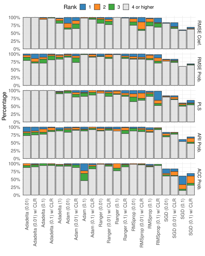
In order to provide insights into the various optimizers’ performance, we conduct a small benchmark study to assess the influence of the choice of an optimizer and to find a good default. Figure 3 visualizes the comparison based on the ranks for each optimizer across all 48 settings from Section 4.1.
Results
Figure 3 indicates that convergence problems are primarily encountered for SGD with a substantial amount of runs diverging during optimization. An overall performance assessment based on ranks indicates that the RMSprop optimizer achieves the lowest overall rank. However, the figure highlights that in fact, no clear best optimizer emerges across all scenarios. The ranks obtained for the different optimizers also vary considerably with the performance criterion.
Overall one might conclude, that both the RMSprop optimizer and the Adam optimizer perform in general well, also when used with their default settings. We note, however, that tuning the optimizer and its learning rate would in general also be beneficial in terms of both predictive performance and estimation quality. A further speed-up for some of these routines can be achieved by additionally incorporating momentum, which also proved to be effective in the optimization of additive models using boosting (Schalk et al, 2022).
4.3 Mixture of Additive Regression Models
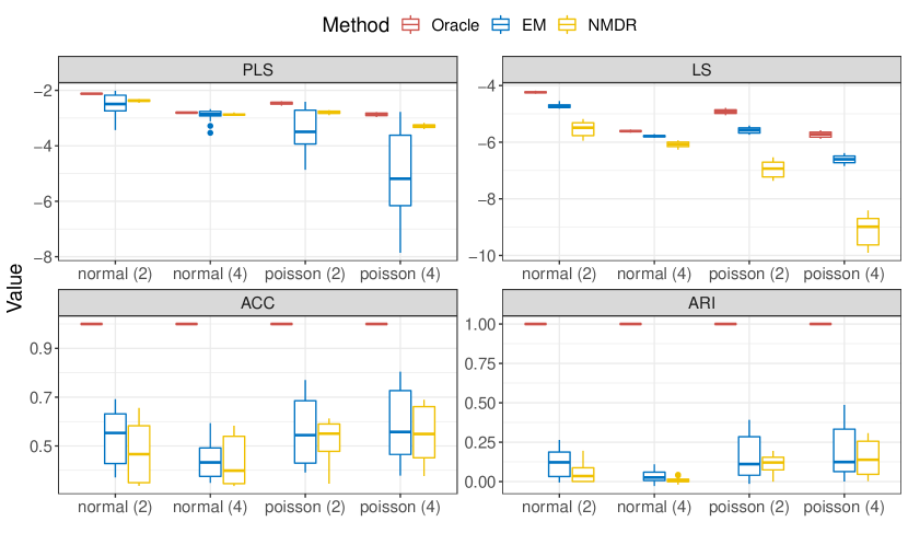
Next, we investigate mixtures of mean regression models with non-linear smooth effects in the additive predictors of the mean distribution parameter. We generate data points from mixtures of Poisson or normal distributions with the additive structured predictor of the means defined by , , and with , , and . All covariates are independently drawn from a uniform distribution . We model those effects using thin-plate regression splines from Wood (2017). For Poisson data, we use and the identity for the Gaussian case. We vary to be either or and add 3 or 10 noise variables that are also included in the model as non-linear smooth predictors for the expectation parameter. We use two different scale values or , which either define the Gaussian variance in each mixture component or a multiplicative offset effect in the Poisson case. Our method is compared with a state-of-the-art implementation of mixtures of additive models using the R package flexmix (Leisch, 2004) and, as an oracle, a generalized additive model with varying coefficients for all smooth effects, where the class label (unknown to the other two approaches) is used as the varying parameter. For NMDR, the smoothing parameters are determined as described in Section 3.3 via the respective degrees-of-freedom which are set equally for all smooths to for normal and for Poisson distribution.
Results
The comparison for all settings is depicted in Figure 4 showing the average log-score (LS; calculated on the training dataset using the estimated model parameters) and PLS, as well as the ARI and ACC. The boxplots summarize all 10 simulation replications for the two different mixture weights and the two number of noise variables settings. Results suggest that our approach leads to better predictions measured by the PLS, but is inferior in terms of LS. The smaller LS values are possibly due to fewer data points to fit the model because of the need for a validation set, and due to the shrinkage induced by early stopping the procedure. The median performance of the clustering induced based on the estimated posterior probabilities is in general on par with the EM-based approach in terms of ARI and ACC with flexmix, while showing even slightly better performance in the Gaussian case.
4.4 Misspecified Mixtures and Sparsity
In this simulation, we use a normal mixture with fixed linear predictors for each distribution and distribution parameter (mean and variance), where all features are again drawn from a standard normal distribution and regression coefficients from a uniform -distribution. The data is then generated using actual mixture components with drawn (independently of features) from a uniform distribution on the interval (0.06, 0.094) and to ensure that the minimum value of both probabilities is at least 6%. We then evaluate the estimation of mixture probabilities by NMDR for when increasing the number of specified distributions . To allow for sparsity in , we use the objective function introduced in Section 3.3. For each scenario, 10 replications are performed.
Results
Results for various settings of the entropy penalty parameter are depicted in Figure 5. While setting to small values larger than zero can improve the predictive performance and even outperform the correctly specified model without additional distribution components, the bias induced by the penalty generally decreases the estimation performance.
We additionally investigate the coefficient path obtained from varying values of the penalty parameter for one simulated example. Results for the setting are depicted in Figure 6. is varied between 0 and 1 on a logarithmic scale. The true model has two non-zero probabilities and while the other entries in are 0.
5 Cell Cycle-regulated Genes of Yeast
In order to demonstrate the flexibility of our approach, we investigate its application to the yeast cell cycle dataset from Spellman et al (1998). In this study, genome-wide mRNA levels were measured for 6178 yeast open reading frames (ORFs) for 119 min at 7 min intervals. We here analyze the subset of data where all 18 time points for the alpha factor arrest are available. The resulting longitudinal dataset consists of 80,802 observations of the standardized expression levels. A subset of this dataset was also analyzed using mixture models in Grün et al (2011).
Distributional Mixture Regression
As both the mean and standard deviation of the standardized expression levels of genes change over time, we apply a mixture of distributional regressions model where the mean and the standard deviation of the normally distributed mixture components depend on time, i.e., for . The additive structured predictors for these distribution parameters are defined as
where the non-linear smooth functions are modeled by thin-plate regression splines (Wood, 2003). Previous approaches for modeling this dataset investigated the use of a mixture of mixed models, i.e., the inclusion of gene-specific random effects (Luan and Li, 2003; Grün et al, 2011). We investigate here an alternative option for modeling this additional heterogeneity by allowing for time-varying standard deviations. We use which corresponds to the number of mixture components identified by Spellman et al (1998).
Results
In order to plot the estimated smooth effects together with the true observations, we first derive the component membership of every gene. As done in the E-step of mixture model approaches (see, e.g., Grün et al, 2011), we calculate the a posteriori probability for every gene to belong to component and then take the maximum of all components . For this application, observations were only assigned to 5 of the 6 assumed components. Note that due to the nature of our optimization routine, not all components necessarily contain at least one observation.
Comparing the number of genes assigned to each cluster one sees that the most common component in our results is cluster 6 with 39,078 observations. Cluster 4 contains 25,722 observations, cluster 1 9,306, and cluster 5 6,552 observations. The least number of observations are assigned to cluster 2 which contains only 144 observations.
Figure 7 visualizes the results obtained in a panel-plot where in each panel the trajectories of the ORFs for all genes assigned to this cluster are shown together with the component-specific estimates of the time-varying means and standard deviations. The identified clusters clearly vary in showing either an initial decrease or increase in their means. In addition, one also sees that the standard deviations of the clusters vary over time with some clusters exhibiting a particularly large amount of heterogeneity at later time points.
6 Outlook
We have introduced the class of mixtures of experts distributional regression with additive structural predictors and investigated its embedding into neural networks for robust model estimation. Overall this leads to the neural mixture of experts distributional regression (NMDR) approach. We show that popular first-order adaptive update routines are well-suited for learning these mixture of experts (distributional) regression models and also highlight that the embedding into a neural network estimation framework allows for straightforward extensions of the general mixture model class and (regularized) maximum-likelihood estimation using optimization routines suitable also for big data applications due to mini-batch training. Using the proposed architecture for mixture of experts distributional regression, a possible extension of our approach is therefore the combination with other (deep) neural networks. This allows learning both the distribution components and the mixture weights either by (a) a structured model, such as a linear or additive model, (b) a custom (deep) neural network, or (c) a combination thereof. A similar approach has been investigated by Fritz et al (2022) using a zero-inflated Poisson model (i.e., a mixture including a point mass distribution) which includes both additive effects and a graph neural network in the additive predictor.
Declarations
The authors declare that they have no known competing financial interests or personal relationships that could have appeared to influence the work reported in this paper.
References
- \bibcommenthead
- Abadi et al (2015) Abadi M, Agarwal A, Barham P, et al (2015) TensorFlow: Large-scale machine learning on heterogeneous systems. URL https://www.tensorflow.org/
- Bishop (1994) Bishop CM (1994) Mixture Density Networks. Aston University
- DeSarbo and Cron (1988) DeSarbo WS, Cron WL (1988) A maximum likelihood methodology for clusterwise linear regression. Journal of Classification 5(2):249–282
- Diebolt and Robert (1994) Diebolt J, Robert CP (1994) Estimation of finite mixture distributions through Bayesian sampling. Journal of the Royal Statistical Society: Series B (Methodological) 56(2):363–375
- Dillon et al (2017) Dillon JV, Langmore I, Tran D, et al (2017) TensorFlow distributions. 10.48550/arXiv.1711.10604
- Fritz et al (2022) Fritz C, Dorigatti E, Rügamer D (2022) Combining graph neural networks and spatio-temporal disease models to improve the prediction of weekly covid-19 cases in germany. Scientific Reports 12(1):1–18
- Frühwirth-Schnatter (2006) Frühwirth-Schnatter S (2006) Finite Mixture and Markov Switching Models. Springer
- Gelfand and Dey (1994) Gelfand AE, Dey DK (1994) Bayesian model choice: Asymptotics and exact calculations. Journal of the Royal Statistical Society: Series B (Methodological) 56(3):501–514
- Glorot and Bengio (2010) Glorot X, Bengio Y (2010) Understanding the difficulty of training deep feedforward neural networks. In: Teh YW, Titterington M (eds) Proceedings of the Thirteenth International Conference on Artificial Intelligence and Statistics, Proceedings of Machine Learning Research, vol 9. PMLR, Chia Laguna Resort, Sardinia, Italy, pp 249–256
- Gormley and Frühwirth-Schnatter (2019) Gormley IC, Frühwirth-Schnatter S (2019) Mixture of experts models. In: Frühwirth-Schnatter S, Celeux G, Robert CP (eds) Handbook of Mixture Analysis. Chapman & Hall/CRC Handbooks of Modern Statistical Methods, Chapman and Hall/CRC, p 271–307
- Grün and Leisch (2007) Grün B, Leisch F (2007) Fitting finite mixtures of generalized linear regressions in R. Computational Statistics & Data Analysis 51(11):5247–5252
- Grün et al (2011) Grün B, Scharl T, Leisch F (2011) Modelling time course gene expression data with finite mixtures of linear additive models. Bioinformatics 28(2):222–228
- Hinton et al (2012) Hinton G, Srivastava N, Swersky K (2012) Neural networks for machine learning. Coursera, video lectures 264(1)
- Hubert and Arabie (1985) Hubert L, Arabie P (1985) Comparing partitions. Journal of Classification 2(1):193–218
- Kingma and Ba (2014) Kingma DP, Ba J (2014) Adam: A method for stochastic optimization. 10.48550/arXiv.1412.6980
- Kneib (2013) Kneib T (2013) Beyond mean regression. Statistical Modelling 13(4):275–303
- Leisch (2004) Leisch F (2004) FlexMix: A general framework for finite mixture models and latent class regression in R. Journal of Statistical Software 11(8):1–18. 10.18637/jss.v011.i08
- Luan and Li (2003) Luan Y, Li H (2003) Clustering of time-course gene expression data using a mixed-effects model with B-splines. Bioinformatics 19(4):474–482
- Magdon-Ismail and Atiya (1998) Magdon-Ismail M, Atiya A (1998) Neural networks for density estimation. In: Advances in Neural Information Processing Systems
- McLachlan and Peel (2004) McLachlan GJ, Peel D (2004) Finite Mixture Models. John Wiley & Sons
- McLachlan et al (2019) McLachlan GJ, Lee SX, Rathnayake SI (2019) Finite mixture models. Annual Review of Statistics and Its Application 6(1):355–378
- Van den Oord and Schrauwen (2014) Van den Oord A, Schrauwen B (2014) Factoring variations in natural images with deep Gaussian mixture models. In: Advances in Neural Information Processing Systems, pp 3518–3526
- Quandt (1958) Quandt RE (1958) The estimation of the parameters of a linear regression system obeying two separate regimes. Journal of the American Statistical Association 53(284):873–880
- R Core Team (2022) R Core Team (2022) R: A Language and Environment for Statistical Computing. R Foundation for Statistical Computing, Vienna, Austria, URL https://www.R-project.org/
- Rigby and Stasinopoulos (2005) Rigby RA, Stasinopoulos MD (2005) GAMLSS: A distributioal regression approach. Journal of the Royal Statistical Society: Series C (Applied Statistics) 54(3):507–554
- Rügamer et al (2020) Rügamer D, Kolb C, Klein N (2020) A unified network architecture for semi-structured deep distributional regression. 10.48550/arXiv.2002.05777
- Rügamer et al (2022) Rügamer D, Kolb C, Fritz C, et al (2022) deepregression: A flexible neural network framework for semi-structured deep distributional regression. Journal of Statistical Software Accepted, https://arxiv.org/abs/arXiv:2104.02705
- Schalk et al (2022) Schalk D, Bischl B, Rügamer D (2022) Accelerated componentwise gradient boosting using efficient data representation and momentum-based optimization. Journal of Computational and Graphical Statistics 0(0):1–11
- Späth (1979) Späth H (1979) Algorithm 39 clusterwise linear regression. Computing 22(4):367–373
- Spellman et al (1998) Spellman PT, Sherlock G, Zhang MQ, et al (1998) Comprehensive identification of cell cycle–regulated genes of the yeast Saccharomyces cerevisiae by microarray hybridization. Molecular Biology of the Cell 9(12):3273–3297
- Stasinopoulos and Rigby (2007) Stasinopoulos DM, Rigby RA (2007) Generalized additive models for location scale and shape (gamlss) in R. Journal of Statistical Software 23(7):1–46
- Stasinopoulos and Rigby (2016) Stasinopoulos M, Rigby B (2016) gamlss.mx: Fitting Mixture Distributions with GAMLSS. R package version 4.3-5
- Stasinopoulos et al (2018) Stasinopoulos MD, Rigby RA, Bastiani FD (2018) GAMLSS: A distributional regression approach. Statistical Modelling 18(3–4):248–273
- Viroli and McLachlan (2019) Viroli C, McLachlan GJ (2019) Deep Gaussian mixture models. Statistics and Computing 29(1):43–51
- Wedel and DeSarbo (1995) Wedel M, DeSarbo WS (1995) A mixture likelihood approach for generalized linear models. Journal of Classification 12(1):21–55
- Wood (2003) Wood SN (2003) Thin plate regression splines. Journal of the Royal Statistical Society: Series B (Statistical Methodology) 65(1):95–114
- Wood (2017) Wood SN (2017) Generalized Additive Models: An Introduction with R. CRC Press
- Wood and Fasiolo (2017) Wood SN, Fasiolo M (2017) A generalized Fellner-Schall method for smoothing parameter optimization with application to Tweedie location, scale and shape models. Biometrics 73(4):1071–1081. https://doi.org/10.1111/biom.12666, URL https://onlinelibrary.wiley.com/doi/abs/10.1111/biom.12666
- Wright (2019) Wright L (2019) New deep learning optimizer, ranger: Synergistic combination of radam lookahead for the best of… Medium
- Zeiler (2012) Zeiler MD (2012) ADADELTA: An adaptive learning rate method. 10.48550/arXiv.1212.5701
- Zong et al (2018) Zong B, Song Q, Min MR, et al (2018) Deep autoencoding Gaussian mixture model for unsupervised anomaly detection. In: International Conference on Learning Representations