SafeBound: A Practical System for Generating Cardinality Bounds

Abstract.

Recent work has reemphasized the importance of cardinality estimates for query optimization. While new techniques have continuously improved in accuracy over time, they still generally allow for under-estimates which often lead optimizers to make overly optimistic decisions. This can be very costly for expensive queries. An alternative approach to estimation is cardinality bounding, also called pessimistic cardinality estimation, where the cardinality estimator provides guaranteed upper bounds of the true cardinality. By never underestimating, this approach allows the optimizer to avoid potentially inefficient plans. However, existing pessimistic cardinality estimators are not yet practical: they use very limited statistics on the data, and cannot handle predicates. In this paper, we introduce SafeBound, the first practical system for generating cardinality bounds. SafeBound builds on a recent theoretical work that uses degree sequences on join attributes to compute cardinality bounds, extends this framework with predicates, introduces a practical compression method for the degree sequences, and implements an efficient inference algorithm. Across four workloads, SafeBound achieves up to 80% lower end-to-end runtimes than PostgreSQL, and is on par or better than state of the art ML-based estimators and pessimistic cardinality estimators, by improving the runtime of the expensive queries. It also saves up to 500x in query planning time, and uses up to 6.8x less space compared to state of the art cardinality estimation methods.

1. Introduction

When considering how to execute a database query, the query optimizer relies on cardinality estimates to determine costs of potential plans and choose an efficient one. Recent benchmarks of query optimizers have shown that (1) traditional cardinality estimators routinely underestimate the true cardinality by many orders of magnitude (Leis et al., 2018) (2) underestimating cardinalities can result in highly inefficient query plans (Leis et al., 2018; Han et al., 2021; Kim et al., 2022) and (3) accurate estimates of large (sub) queries are crucial to generating good query plans (Han et al., 2021).

These observations have motivated work on cardinality bounding, also called pessimistic cardinality estimation, where the cardinality estimator provides guaranteed upper bounds of the true cardinality rather than unbiased estimates (Cai et al., 2019; Hertzschuch et al., 2021). When given a cardinality bound rather than a cardinality estimate and assuming a reasonably accurate cost model, the query optimizer will avoid the most inefficient query plans, e.g. choosing a nested loop join between two large tables. Formulas that bound the output cardinality of a query have been introduced in the theoretical community (Grohe and Marx, 2006; Gottlob et al., 2012; Khamis et al., 2016, 2017; Deeds et al., 2022), and implementations based on simplified versions of these formulas are described in (Cai et al., 2019) and in (Hertzschuch et al., 2021). One comprehensive study of cardinality estimation methods reports good end-to-end performance by cardinality bounds compared to other methods (Han et al., 2021). Recent work has even found novel connections between these cardinality bounds and more traditional estimators, allowing cardinality bounding optimizations to be applied to traditional estimates (Chen et al., 2022). However, current techniques for cardinality bounds produce loose estimates and do not support predicates in queries. In this work, we overcome these limitations and describe, SafeBound, a practical system that uses a rich collection of statistics to generate bounds and supports a wide range of predicates.

To place SafeBound in context, we briefly review the landscape of cardinality estimation techniques. Prior work falls in three broad categories: traditional methods, ML methods, and cardinality bounding methods. Traditional methods are supported by all major database systems and rely on histograms, distinct counts, and most-common-value lists, combined with strong assumptions (uniformity, independence, inclusion of values). These methods are fast and space efficient but suffer from the drawbacks listed above. Also under this umbrella are sampling-based methods, which cope with non-uniformity and correlations, but use indexes during estimation and do not scale to queries with many joins. To compensate for this, a great deal of recent work has gone into creating increasingly complex ML models that automatically detect these correlations (Yang et al., 2020a; Kipf et al., 2019; Wang et al., 2021b; Liu et al., 2021; Zhu et al., 2021; Kim et al., 2022; Woltmann et al., 2019, 2020; Wu and Cong, 2021; Wang et al., 2021a) . While this is certainly an exciting approach and has yielded high accuracy estimates on existing benchmarks, many practical hurdles remain: they require a large memory footprint, have a slow training time, and are hard to interpret (Wang et al., 2021b; Kim et al., 2022; Han et al., 2021). Further, these approaches generally treat under and overestimation identically, which can result in a disconnect between their accuracy and their effect on workload runtime (Negi et al., 2021; Kim et al., 2022).

Previous efforts in cardinality bounding have resulted in good workload runtimes. However, they have been either unable to handle predicates and slow to perform inference or inaccurate and unable to produce guaranteed bounds. PessEst  (Cai et al., 2019) hash-partitions each relation and calculates its bound using the cardinality and max degree for each partition. In order to handle predicates, they resort to scanning base tables at inference time, an unacceptable overhead for query optimizers. Further, the inference time grows exponentially in the total number of partitions. Simplicity (Hertzschuch et al., 2021) uses the same bound as (Cai et al., 2019), but without any hash refinement. Instead, they focus on producing single-table estimates through sampling. However, this results in loose bounds and no longer produces a guaranteed upper bound on the query’s cardinality (see Fig. 5(c)).

Our work draws inspiration from a recent theoretical result (Deeds et al., 2022), which describes an upper bound formula using the degree sequences of all join attributes; this is called the Degree Sequence Bound, DSB. The degree sequence of an attribute is the sorted list $f_{1}\geq f_{2}\geq\cdots\geq f_{d}$ of the frequencies of distinct values in that column: we illustrate it briefly in Fig. 1 and define it formally in Sec. 2. The degree sequence captures a rich set of statistics on the relation: the cardinality is $\sum_{i}f_{i}$, the maximum frequency is $f_{1}$, the number of distinct values is $d$, etc. The memory footprint of the full degree sequence is too large, but it can be compressed using a piecewise constant function $\hat{f}$ such that $f\leq\hat{f}$ (see Fig. 1), thus the technique offers a tradeoff between memory and accuracy. The authors in (Deeds et al., 2022) describe a mathematical upper bound on output cardinality given in terms of the compressed degree sequences. However, the theoretial formalism is not practical: it ignores predicates; the proposed compression definition artificially increases the cardinality of the relation; and there is no concrete compression algorithm.

In this paper, we describe SafeBound, the first practical system for generating cardinality bounds from degree sequences. Like any cardinality estimator, SafeBound has an offline and an online phase (Sec. 3.1). During the offline phase it computes several degree sequences, then compresses them. Unlike (Deeds et al., 2022), we also compute degree sequences conditioned on predicates: SafeBound supports equality predicates, range predicates, LIKE, conjunctions, and disjunctions (Sec. 3.2). Next, we describe a stronger compression method by upper bounding the cumulative degree sequence rather than the degree sequence, and prove that it preserves the cardinalities of the base tables, yet still leads to a guaranteed upper bound on the query’s output cardinality (Sec. 3.3). Any compression necessarily looses some precision, and no compression is optimal for all queries. Thus, we describe a heuristic-based compression algorithm in Sec. 3.4. At the end of the offline phase of SafeBound we have a set of compressed degree sequences. Next, during the online phase, SafeBound takes a query consisting of joins and predicates, and computes a guaranteed upper bound on its output cardinality, using the compressed degree sequences. For this purpose we implemented an algorithm (inspired by (Deeds et al., 2022)) that computes the upper bound in almost-linear time in the total size of all compressed degree sequences. In addition to these fundamental techniques, we describe several optimizations in Sec. 4. Finally, we evaluate SafeBound empirically in Sec. 5. Across four workloads, SafeBound achieves up to 80% lower end-to-end runtimes than PostgreSQL, and is on par or better than state of the art ML-based estimators and pessimistic cardinality estimators. Its performance gains come especially from the expensive queries, because its guarantees on the cardinality prevent the optimizer from making overly optimistic decisions. In the tradeoff between accuracy and build time, SafeBound aims for accuracy. This results in slower build times than Postgres although it is 2-20x faster to build than state of the art ML methods. SafeBound also saves up to 500x in query planning time, and uses up to 6.8x less space compared to state of the art cardinality estimation methods.

In summary, this paper makes the following contributions:

• SafeBound Design: We describe the architecture of SafeBound, the first practical system for cardinality bounds, in Sec. 3.1.

• Predicates: We introduce a scheme for conditioning degree sequences on predicates (Sec. 3.2).

• Valid Compression: We describe an improved compression of degree sequences that preserves the cardinality of the base tables and still leads to a guaranteed upper bound (Sec. 3.3).

• Compression Algorithm: We present an algorithm for compressing a degree sequence with minimal loss (Sec. 3.4).

• Optimizations: We describe several optimizations in Sec. 4.

• Experimental Evaluation: We perform a thorough experimental evaluation on the JOB-Light, JOB-LightRanges, JOB-M, and STATS-CEB benchmarks demonstrating SafeBound’s fast inference, low memory overhead, and nearly optimal workload runtimes across all benchmarks. Sec. 5

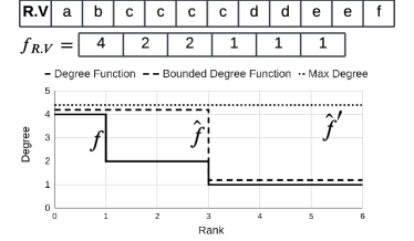
Figure 1. An example column, $R.V$, and its degree sequence $f$. The degree sequence can be compressed by upper bounding it with a step function. We show two step functions, $\hat{f}$ with 2 segments and $\hat{f}^{\prime}$ with 1 segment: $f\leq\hat{f}\leq\hat{f}^{\prime}$. Notice that they will overestimate the total cardinality of the relation, from the true cardinality 11, to 15, and to 24, respectively.

2. Problem Definition and Background

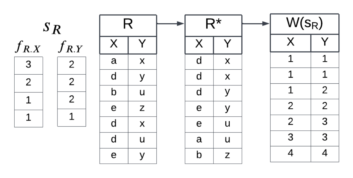
Figure 2. This figure shows the conversion of an input table $R(X,Y)$ to the worst-case instance $W(s_{R})$ which has the same degree sequences but produces larger join outputs. This requires first sorting the columns individually by frequency then re-labeling join values in order of frequency.

2.1. The Cardinality Bounding Problem

Let $Q=R_{1}(\bm{V}_{1})\wedge\ldots\wedge R_{k}(\bm{V}_{k})\wedge P_{1}\wedge\ldots\wedge P_{l}$ be a query, expressed using datalog notation, over relations $R_{i}\in\bm{R}$ with variables $\bm{V}_{i}\subseteq\bm{V}$ and sets of predicates $\bm{P}_{1}\ldots\bm{P}_{l}$. To match the setting of (Deeds et al., 2022), we generally assume that queries are acyclic and that any join between two relations is on a single attribute. These queries, called Berge-acyclic queries, include many natural queries, like chain, star, snowflake queries (Fagin, 1983). However, we go on to provide extensions to handle general queries as well in Sec. 3.6. We further assume that $Q$ is a full conjunctive query, i.e. select * in SQL, and uses bag semantics: both the input relations and the output are bags. Our goal is to compute a bound on its output.

Let $D$ be a database instance with statistics $s$. The goal of cardinality bounding is to generate a bound $B(Q,s)$ such that the following is true,

(1) $$\max_{D\models s}|Q(D)|\leq B(Q,s)$$

The bound, $B(Q,s)$, guarantees that the query $Q$ will have true cardinality less than $B(Q,s)$ when executed on any database consistent with the given statistics, $s$, which we denote $D\models s$. We say that a bound $B(Q,s)$ is tight if there exists a database $D$ consistent with $s$ for which the inequality (1) is an equality. In this paper, $s$ will specifically refer to the degree sequences.

2.2. The Degree Sequence

The core statistic in our system, SafeBound, is the degree sequence (DS), so we describe it in detail here. Consider a variable $V$ (a.k.a. column) of a relation $R$ with domain $\mathbb{D}_{V}$ and values $v\in\mathbb{D}_{V}$. The frequency of a particular value $v$ in relation $R$ is $|\sigma_{V=v}(R)|$. Ranking the values in descending order by frequency, we get a list of values $v^{(1)},\ldots,v^{(|\mathbb{D}_{V}|)}$ whose frequencies, $f_{R.V,i}\stackrel{{\scriptstyle\text{def}}}{{=}}|\sigma_{V=v^{(i)}}(R)|$, form the degree sequence of $R.V$: $f_{R.V,1}\geq f_{R.V,2}\geq\cdots$ The index $i$ is called the rank. The cumulative degree sequence, CDS, is the running sum of the DS, i.e. $F_{R.V,i}\stackrel{{\scriptstyle\text{def}}}{{=}}\sum_{j=1}^{i}f_{R.V,j}$. In the other direction, the DS can be defined as the discrete derivative of the CDS, $f_{R.V,i}=\Delta_{i}F_{R.V,i}=F_{R.V,i}-F_{R.V,i-1}$.

In this paper, we often manipulate these sequences as piecewise functions and may use the following notation, $f_{R.V}(i)=f_{R.V,i}$ and $F_{R.V}(i)=F_{R.V,i}$, for the DS and CDS, respectively. The set of DSs for a relation $R$ will be denoted by $s_{R}$, and the set of DSs for all relations by $s$; similarly, $S_{R}$ and $S$ stand for the CDSs of one relation, or all relations. Let $s,\hat{s}$ be two sets of statistics; we write $s\leq\hat{s}$ to mean that $f_{R.V}(i)\leq\hat{f}_{R.V}(i)$ for all relations $R$, attributes $V$, and ranks $i$. Given a set of statistics $\hat{s}$ and a database $D$, we say that $D$ is consistent with $\hat{s}$ if $s(D)\leq\hat{s}$, where $s(D)$ are the degree sequences for the instance $D$. An example of these concepts can be seen in Figure 1. At the top are the actual values of a column $R.V$ of the database, and below is the degree sequence: the value $4$ corresponds to $c,c,c,c$, the values $2,2$ correspond to $d,d$ and $e,e$, etc. The graph shows the degree sequence $f$ as a solid line. In general, the degree sequence can be large. For the purpose of computing an upper bound of the size of the query, it suffices to compress the DS by upper bounding it using a piecewise constant function: two such functions are shown in the figure, $f\leq\hat{f}\leq\hat{f}^{\prime}$.

2.3. The Degree Sequence Bound

Previous work (Deeds et al., 2022) described a method to compute a tight upper bound on the query’s output from the degree sequences, called the degree sequence bound, DSB, which we briefly describe here.

The Worst-Case Instance: The DSB is defined in terms of a worst-case relation, $W(s_{R})$, associated with the statistics $s_{R}$, and the worst-case instance of the database, $W(s)$, consisting of all relations $W(s_{R})$. These relations are defined such that the size of any query’s answer on $W(s)$ is an upper bound of its size on any database consistent with $s$; in this sense, $W(s)$ is the “worst” instance. Because degree sequences do not capture the correlation between columns within relations or between relations, the worst-case assumption is that the frequency of values is perfectly correlated across columns both within and between relations: i.e., high frequency values occur in the same tuples within relations and join with high frequency values across relations.

We illustrate how to produce a worst-case relation $W(s_{R})$ from a binary relation $R(X,Y)$ in Figure 2. While we are given only the statistics $s_{R}$, i.e. the two degree sequences $f_{R.X},f_{R.Y}$, we also show an instance $R$, to help build some intuition into $W(s_{R})$. First, we sort each column independently by frequency to produce $R^{*}$. This ensures that high-frequency values occur in the same tuples. Next, we relabel our join values in order of frequency to produce $W(s_{R})$, i.e. $x^{(1)}=1,x^{(2)}=2,\ldots$. This ensures that, when we join, say, $R$ and $T$, the high-frequency values in $W(s_{R})$ will join with the high-frequency values in $W(s_{T})$.

The Degree Sequence Bound: The DSB is the size of the query $Q$ run on the worst-case instance $W(s)$, in other words, $|Q(W(s))|$. The following is shown in (Deeds et al., 2022):

Theorem 2.1.

Suppose $Q$ is a Berge-acyclic query, and let $s$ be a set of degree sequences, one for each attribute of each relation. Then, the following is true,

(2) $$\forall D\models s\quad|Q(D)| \leq|Q(W(s))|$$

Further, $W(s)\models s$, which proves that the bound in (2) is tight.

The theorem forms the theoretical basis for compression. Suppose that $\hat{s}$ is a compressed (lossy) representation of $s$, such that $s\leq\hat{s}$. For example, $\hat{s}$ may replace the degree sequences with piecewise constant functions with a small number of segments, as in Fig 1. Then $|Q(W(\hat{s}))|$ is still an upper bound for $Q(D)$, because $D\models s$ implies $D\models\hat{s}$, and we apply the theorem to $\hat{s}$.

2.4. Discussion

In summary, the theory in (Deeds et al., 2022) introduced the DSB, and suggested compressing the degree sequences; they also described an efficient algorithm for the DSB, which we implemented (reviewed in Sec. 3.5). Using degree sequences for cardinality bounding is attractive, because they capture several popular statistics used in cardinality estimation: the number of distinct values in a column $R.V$ is $\|f_{R.V}\|_{0}$; the cardinality of the relation $R$ is $\|f_{R.V}\|_{1}$; and the maximum degree (or maximum frequency) is $\|f_{R.V}\|_{\infty}$. However, the framework in (Deeds et al., 2022) is impractical, for several reasons:

1. The DSB in Theorem 2.1 does not take predicates into account; if the query contains some predicate, e.g. $R.B=2$, then the DSB simply ignores it, which means that the upper bound in Equation (2) will be a huge overestimate.

2. If the compressed sequences $\hat{s}$ dominate $s$, i.e. $s\leq\hat{s}$, then they artificially increase the estimated cardinality of the relations, which increases the DSB.

3. While it describes a bound based on compressed degree sequences, no concrete algorithm for compressing degree sequences is suggested in (Deeds et al., 2022).

In this paper, we make several contributions to address these limitations, and describe SafeBound, a practical cardinality bounding system.

3. SafeBound

In this section, we present SafeBound, the first practical system for cardinality bounding, which is based on several extensions of the results in (Deeds et al., 2022). We start with an overview of SafeBound.

3.1. Overview

SafeBound has an offline and an online phase. During the offline phase the system computes the degree sequences of every join-able attribute of every relation (keys and foreign keys). In addition it also considers a variety of predicate types on each relation, and computes refined degree sequences conditioned on those predicates: this is described in Sec. 3.2. The last step of the offline phase consists of compressing the degree sequences; this is described in Sec. 3.4. Rather than directly compressing the degree sequence as allowed by (Deeds et al., 2022), it compresses the cumulative degree sequence which does not inflate the cardinality of the relation and requires a new correctness proof. This is described in Sec. 3.3. During the online phase, SafeBound receives a query, as defined in Sec. 2, and computes an upper bound on the query’s output using the pre-computed compressed degree sequences. It does not apply the formula in Theorem 2.1 naively, but, instead, it implements a fast algorithm that runs in time proportional to the total size of the compressed sequences; this is described in Sec. 3.5.

Example 3.1.

We will refer to the following running example:

$$Q\stackrel{{\scriptstyle\text{def}}}{{=}} R(X,A,B)\wedge S(X,Y,C)\wedge T(Y)$$

$$\wedge (A<5)\wedge(B=2)\wedge(C\,\,\texttt{LIKE '\%Abdul\%'})$$

During the offline phase (before the query arrives) SafeBound computes the degree sequences for $R.X,R.A,\ldots,T.Y$, as well as degree sequences conditioned on predicates, e.g. degree sequences of $R.X$ conditioned on range predicates applied to $R.A$. All these degree sequences are compressed and stored. During the online phase, SafeBound takes the query $Q$ above, and uses all available degree sequences to compute an upper bound to the query’s output.

We will use the following terminology. A column to which a predicate is applied is called a filter column; a column used in a join is called a join column. Note that a column can be both a filter column and a join column.

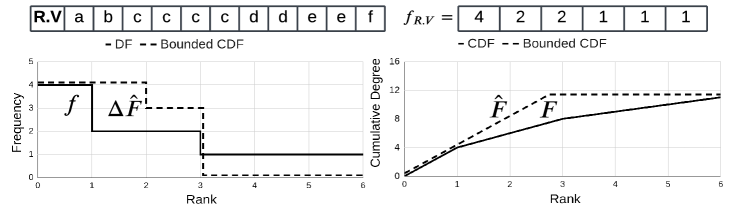
Figure 3. We show here how to compress the CDS of the column Fig. 1. The degree sequence $f$ on the left has the cumulative degree sequence $F$ on the right. We upper bound the latter by $\hat{F}$, a piecewise linear function with two segments. Notice that the cardinality of the relation is preserved: $|R|=F(6)=\hat{F}(6)=11$. The degree sequence $\hat{f}\stackrel{{\scriptstyle\text{def}}}{{=}}\Delta\hat{F}$ associated to $\hat{F}$ no longer dominates the original $f$. Yet, Theorem 3.1 proves that we can still use $\hat{f}$ to compute an upper bound on the cardinality of a query.

3.2. Conditioning on Predicates

Predicates in a query can significantly reduce the cardinality of the output. SafeBound accounds for predicates by computing additional degree sequences for each join column by conditioning on predicates. SafeBound supports five types of predicates: equality, range, conjunctions, LIKE, and disjunctions. In this section we assume that all degree sequences are exact; once we replace them with compressed sequences in the next section, we will discuss some minor adjustments to the formulas introduced here.

Equality Predicates: The main idea is the following. Let $V$ be a join column of a relation $R$, and consider a query that includes an equality predicate, $R.A=a_{k}$, for some constant $a_{k}\in\mathbb{D}_{A}$. If we ignore the predicate and compute the upper bound of the query without this predicate, then we massively overestimate the query’s cardinality. There are two extreme ways to account for the equality predicate. At one extreme, we could compute a separate degree sequence, $f_{R.V|(A=a_{\ell})}$, for each value $a_{1},a_{2},\ldots\in\mathbb{D}_{A}$ from the subset $\sigma_{A=a_{\ell}}(R)$. At query estimation time, we use the degree sequence $f_{R.V|(A=a_{k})}$ instead of the unconditioned sequence $f_{R.V}$. But this approach is prohibitive, because it requires storing a large number of degree sequences. At the other extreme, we could store only the max of all these individual degree sequences,

(3) $$f_{R.V|A}\stackrel{{\scriptstyle\text{def}}}{{=}} \max_{\ell}f_{R.V|(A=a_{\ell})}$$

and use this to estimate the query’s upper bound. This uses very little space, only one DS which we use for every equality predicate on $A$, no matter the constant $a_{k}$. But this may lead to significant over-approximations of the upper bound. SafeBound adopts a compromise. For each attribute $A$, it computes a Most Common Value (MCV) list, computes separate degree sequences for $V$ conditioned on each of these values, and computes one default DS, given by formula (3), where $a_{\ell}$ ranges over non-MCV values. At estimation time, if $a_{k}$ is in the MCV list then we use its own degree sequence, otherwise we use the default one. In our system, we chose between $1000$ and $5000$ values to include in every MCV list. We will slightly revisit Eq. (3) in the next section.

Range Predicates: To handle range predicates, SafeBound uses a data structure that builds on the idea of traditional histograms. The naive way to do this is to compute an equi-depth histogram over $R.A$ where each bucket stores the degree sequence of $R.V$ restricted to that bucket. However, a range predicate may overlap multiple buckets which would require us to return the summation of the degree sequences in those buckets. This summation artificially inflates the highest frequency values, increasing the DSB significantly. Instead, we build a hierarchy of equi-depth histograms with $2^{k},2^{k-1},\ldots,2^{1}$ buckets. At query time, we identify the smallest bucket which fully encapsulates the range query and return the degree sequence stored there. In our system, we typically used $k=7$.

Conjunctions: Suppose that the query contains a conjunction of predicates on the same relation $R$: $P_{1}(R.A)\wedge P_{2}(R.B)\wedge\cdots$ For each predicate, we have computed a degree sequence conditioned on that predicate, $f_{R.V|A},f_{R.V|B},\ldots$ Then, we take their minimum:

(4) $$f_{R.V|(A\wedge B\wedge\cdots)}(i)\stackrel{{\scriptstyle\text{def}}}{{=}}\min(f_{R.V|A}(i),f_{R.V|B}(i),\ldots)$$

Referring to our running Example 3.1, there are two predicates on $R$. The degree sequence $f_{R.X}$ conditioned on the conjunction is $f(i)\stackrel{{\scriptstyle\text{def}}}{{=}}\min(f_{R.X|(A<5)}(i),f_{R.X|(B=2)}(i))$.

LIKE Predicates: SafeBound converts a predicate $R.A\ \texttt{LIKE'\%xyzu\%'}$ into a conjunction of predicates on 3-grams. For every attribute $R.A$ of type text, SafeBound first computes an MCV list of 3-grams that occur in $A$ and calculates the degree sequences of $R.V$ conditioned on all 3-grams that occur in the MCV. Separately, it calculates the degree sequence of $R.V$ conditioned on $A$ not containing any 3-gram in the MCV. At query time, we split the text in the LIKE predicate into 3-grams, then compute the $\min$ of all degree sequences conditioned on each 3-gram that occurs in the MCV list. If none of the predicate’s 3-grams appear in this list, we use the degree sequence conditioned on not containing common 3-grams. Referring to our running Example 3.1, the string ’%Abdul%’ is split into the 3-grams Abd, bdu, dul; for each 3-gram we retrieve the degree sequence $S.X$ conditioned on that 3-gram, then compute their min (or take the default if none of them are in the MCV list); we apply the same process to compute the degree sequence of $S.Y$.

Disjunctions: Suppose a query has a disjunction of predicates over a relation $R$, $P_{1}(R.A_{1})\vee\cdots\vee P_{k}(R.A_{k})$. For each predicate we have the degree sequence of $R.V$ conditioned on it; then, we take their sum. For example, the IN predicate in SQL is treated as a disjunction: the degree sequence condition on of $R.A\text{ IN ['a','b','c']}$ is $f_{R.V|(A=a)}+f_{R.V|(A=b)}+f_{R.V|(A=c)}$.

Example 3.2.

The Title relation in the JOBLightRanges benchmark has 7 filter columns (episode_nr, season_nr, production_year, series_years, phonetic_code, series_years, imdb_index) and two join columns (id, kind_id). This results in seven histograms, MCV lists, and, for the string attributes, 3-gram lists which store 2 degree sequences per bin, MCV, and tri-gram, respectively. In total, there are $18,522$ degree sequences for the relation Title, each describing a subset of the table. This motivates our compression technique in Sec. 3.3 and 3.4, and the group compression in Sec. 4.1.

Discussion: SafeBound computes DS’s only for join columns (keys and foreign keys), each conditioned on every filter column. In theory this could lead to $O(n^{2})$ DS’s for a table with $n$ attributes, but in practice, a typical table has $O(1)$ foreign keys, resulting in $O(n)$ DS’s per table.

3.3. Valid Compression

The degree sequence statistics, $s$, are as large as the database instance, $D$, hence they are impractical for cardinality estimation. SafeBound compresses each degree sequence using a piecewise constant function with a small number of segments. We denote by $\hat{s}$ the collection of compressed degree sequences. As we saw in Theorem 2.1, the theoretical results in (Deeds et al., 2022) required $D\models\hat{s}$, meaning that that every degree sequence $f_{R.V}$ of the database $D$ is dominated by the corresponding DS in $\hat{s}$: $f_{R.V}(i)\leq\hat{f}_{R.V}(i)$. The problem is that, if we increase the degree sequence $f_{R.V}$ to $\hat{f}_{R.V}$, then the cardinality of the worst case relation $W(\hat{s}_{R})$ will increase artificially, from $\sum_{i}f_{R.V}(i)$ to $\sum_{i}\hat{f}_{R.V}(i)$. This leads to poor upper bounds. In this section we introduce a stronger compression method, which does not increase the cardinality of the worst case instance.

Our new idea is that, instead of dominating the degree sequence, $f_{R.V}\leq\hat{f}_{R.V}$, we will dominate the cumulative degree sequence $F_{R.V}(i)\leq\hat{F}_{R.V}(i)$. Obviously, if the DS is dominated, then the CDS is dominated too, in other words $f_{R.V}\leq\hat{f}_{R.V}$ implies $F_{R.V}\leq\hat{F}_{R.V}$, but the converse does not hold in general, as is illustrated in Fig. 3. The advantage is that we can dominate the CDS yet still preserve the cardinality, by ensuring $|R|=F_{R.V}(|\mathbb{D}_{V}|)=\hat{F}_{R.V}(|\mathbb{D}_{V}|)$, see Fig. 3, but the problem is that we can no longer use Theorem 2.1 to conclude that the compressed sequence leads to an upper bound. We show that the upper bound still holds, by proving the new theorem below. We denote a collection of CDS by $\hat{S}$, and write $D\models\hat{S}$ if every CDS of $D$ is dominated by the corresponding CDS in $\hat{S}$. Recall that $\Delta F(i)\stackrel{{\scriptstyle\text{def}}}{{=}}F(i)-F(i-1)$, thus $\Delta\hat{S}$ represents the DS associated to the CDS in $\hat{S}$.

Theorem 3.1.

Suppose $Q$ is a Berge-acyclic query, and let $\hat{S}$ be a set of cumulative degree sequences, one for each relation and each attribute. Then, the following is true,

(5) $$\forall\,D\models\hat{S}\quad|Q(D)|\leq|Q(W(\Delta\hat{S}))|$$

The proof of this new theorem is a non-trivial extension of Theorem 2.1, and uses some results from (Deeds et al., 2022) as well as new results; we defer it to our online appendix (Anonymized authors for double blind reviewing, 2022). This justifies the following:

Definition 3.3.

Let $R.V$ be a column with degree sequence $f_{R.V}$. We say that $\hat{f}$ is valid for $f_{R.V}$ if (a) it is a degree sequence, meaning it is non-increasing, $\hat{f}(i-1)\geq\hat{f}(i)$, (b) its CDS $\hat{F}(i)\stackrel{{\scriptstyle\text{def}}}{{=}}\sum_{j\leq i}\hat{f}(i)$ dominates the CDS of $R.V$: $F_{R,V}(i)\stackrel{{\scriptstyle\text{def}}}{{=}}\sum_{j\leq i}f_{R.V}(i))\leq\hat{F}(i)$, $\forall i$, (c) it preserves the cardinality $|R|=F_{R.V}(|\mathbb{D}_{V}|)=\hat{F}(|\mathbb{D}_{V}|)$.

To summarize, SafeBound compresses every DS $f_{R.V}$ into a valid DS $\hat{f}_{R.V}$. Since $\hat{f}_{R.V}$ no longer dominates $f_{R.V}$, we need to make some small adjustments to the way we compute conditioned degree sequences in Sec. 3.2, as follows. The max-degree sequence for the non-MCV values, Eq. (3), will be computed over CDS rather than DS, in other words we replace it with $\hat{F}_{R.V|A}\stackrel{{\scriptstyle\text{def}}}{{=}}\max_{\ell}\hat{F}_{R.V|(A=a_{\ell})}$: this, improves the bound. The min-degree sequence for a conjunction of predicates in Eq. (4) will also use the CDS, in other words it becomes $\hat{F}_{R.V|(A\wedge B\wedge\cdots)}(i)\stackrel{{\scriptstyle\text{def}}}{{=}}\min(\hat{F}_{R.V|A}(i),\hat{F}_{R.V|B}(i),\ldots)$: this worsens the bound, but this is necessary to ensure correctness. All other computations remain unchanged, with each $f$ replaced by $\hat{f}$. Next, we discuss how to compute a good valid compression for a given degree sequence.

3.4. The Compression Algorithm

In this section, we describe the compression algorithm of a degree sequence $f$ to $\hat{f}$. Function approximations are defined by a model class (e.g. polynomial, sinusoidal, etc), a loss function (e.g. mean squared error), and an approximation algorithm (e.g. gradient descent, convex hull, etc). We have three requirements: (1) the approximation of the CDS must be an upper bound of the original CDS, i.e. $F\leq\hat{F}$ (by Th. 3.1), (2) the model class must be closed under both multiplication with the derivative and composition, and (3) the model class must be invertible. The last two requirements are needed by Algorithm 2, which is described in the next section. Given these requirements, SafeBound uses piecewise linear representation for $\hat{F}$, or, equivalently, piecewise constant for $\hat{f}$:

Definition 3.2.

A function $f(x)$ is $k$-piecewise linear over the domain $(m_{0},m_{k}]$ if there exist tuples $\{(m_{0},m_{1},a_{1}x+b_{1}),\ldots,$
$(m_{k-1},m_{k},a_{k}x+b_{k})\}$ such that $f(x)=a_{i}x+b_{i}\,\,\forall x\in(m_{i-1},m_{i}]$
$\forall 1\leq i\leq k$. We call the values, $m_{0},\ldots,m_{k}$, dividers and call each interval, $(m_{\ell-1},m_{\ell}]$, a segment. When $a_{1}=\cdots=a_{k}=0$, we say that $f$ is piecewise constant.

Every piecewise linear function with $k$ segments can be stored in $O(k)$ space. If $\hat{f}$ is piecewise constant, then $\hat{F}(i)\stackrel{{\scriptstyle\text{def}}}{{=}}\sum_{j\leq i}\hat{f}(j)$ is piecewise linear, and, conversely, if $\hat{F}$ is piecewise linear and continuous, then $\hat{f}\stackrel{{\scriptstyle\text{def}}}{{=}}\Delta\hat{F}$ is piecewise constant. SafeBound compresses degree sequences as piecewise constant, or, equivalently compresses cumulative degree sequences as piecewise linear functions; the conversion from one to the other is done in time $O(k)$.

Degree sequences naturally compress very well. If $R.V$ is a key, then its degree sequence $f(1)=f(2)=\cdots=f(N)=1$ compresses losslessly to a single segment, $k=1$. Even if $R.V$ is not a key, its degree sequence can still be compressed losslessly:

Lemma 3.3.

Let $f$ be the degree sequence of a column $R.V$, and suppose $R$ has $N$ tuples. Then $f$ compresses losslessly to a piecewise constant function with $k\leq\min(\sqrt{2N},f(1))$ segments.

Proof.

We have $f(1)\geq f(2)\geq\cdots\geq f(d)$, where $d$ is the number of distinct values in $R.V$. Assume w.l.o.g. that $f(d)>0$ (otherwise, decrease $d$). Consider its natural dividers into $k$ segments, $0=i_{0}<i_{1}<\ldots<i_{k}\stackrel{{\scriptstyle\text{def}}}{{=}}d$ such that $f(j)$ is constant for $i_{\ell-1}<j\leq i_{\ell}$ and $f(i_{1})>\cdots>f(i_{k})>0$. Since $f$ takes integer values, it follows that $f(1)=f(i_{1})\geq k$. On the other hand, $|R|=\sum_{i}f(i)\geq f(i_{1})+\cdots+f(i_{k})\geq k+(k-1)+\cdots+1+0=k(k+1)/2\geq k^{2}/2$, which implies $k\leq\sqrt{2N}$. This proves $k\leq\min(\sqrt{2N},f(1))$. ∎

Algorithm 1 ValidCompress

0:  $f_{R.V},c$ // $f_{R.V}=$ exact DS, $c=$ accuracy parameter

1:  $d=|\mathbb{D}_{R.V}|$ // the number of distinct values in $R.V$

2:  $SJ=\sum_{i=1}^{d}(f_{R.V}(i)^{2})$ // exact DSB of selfjoin

3:  // initialize 1st segment $(m_{0},m_{1}]$:

4:  $k=1;\epsilon_{1}=0;m_{0}=m_{1}=0$; $a_{1}=f_{R.V}(1);b_{1}=0$

5:  for $i\in[1,\ldots,d]$ do

6:     $\epsilon_{k}=\epsilon_{k}+a_{k}^{2}\cdot(f_{R.V}(i)/a_{k})-f_{R.V}(i)^{2}$

7:     if $\epsilon_{k}\geq c\cdot SJ$ then

8:        // DSB error too big?

9:        $k=k+1;\epsilon_{k}=0$ // start new segment $(m_{k-1},m_{k}]$

10:        $m_{k}=m_{k-1};a_{k}=f_{R.V}(i);b_{k}=b_{k-1}+a_{k-1}(m_{k-1}-m_{k-2})$

11:     end if

12:     $m_{k}=m_{k}+f_{R.V}(i)/a_{k}$ // extend segment $(m_{k-1},m_{k}]$

13:  end for

14:  $\hat{F}_{R.V}=\{\left(m_{l-1},m_{l},a_{l}(x-m_{l-1})+b_{l}\right)|l=1,k\}\cup\{(m_{k},d,|R|)\}$

15:  return  $\hat{f}_{R.V}\stackrel{{\scriptstyle\text{def}}}{{=}}\Delta\hat{F}_{R.V}$ // $k+1$ segments

SafeBound does not rely on the natural compression, but instead uses a more aggressive, lossy compression, with a much smaller number of segments than given by the lemma. Algorithm 1, called ValidCompress, takes as input a degree sequence $f_{R.V}$, and an accuracy parameter $c>0$, and computes a valid compression using the following heuristic: if $SJ=\sum_{i=1}^{|\mathbb{D}_{V}|}f_{R.V}(i)^{2}$ is the exact Degree Sequence Bound of the self-join on the column $R.V$, then the algorithm ensures that no segment increases the DSB by more than $c\cdot SJ$.

We describe the algorithm and prove its correctness. It iterates through the degree sequence $f_{R.V}(i)$, $i=1,2,3,\ldots$ and builds the segments of $\hat{F}_{R.V}$ one by one: $(m_{0}\stackrel{{\scriptstyle\text{def}}}{{=}}0,m_{1}],(m_{1},m_{2}],\ldots,(m_{k-1},m_{k}]$. Initially, $k=1$, the first segment is empty $(0,0]$, and the initial slope is $a_{1}=f_{R.V}(1)$. The for-loop in lines 5-13 iterates over each rank $f_{R.V}(i)$ and does one of two things: it either extends the current segment $(m_{k-1},m_{k}]$ by increasing $m_{k}$ (line 12), or it increases $k$ and starts a new empty segment (line 9), which is also immediately extended in line 12. The choice between these actions is dictated by our heuristics: ensure that each segment contributes at most $c\cdot SJ$ to the DSB. We prove that, regardless of the heuristic, the algorithm always computes a valid compression, by checking conditions (a), (b), (c) in Def. 3.3. The following invariant holds at the beginning of each iteration of the for-loop (line 5): if $\hat{F}_{R.V}$ denotes the current piecewise linear function, defined on $(0,m_{k}]$, then:

$$\hat{F}_{R.V}(m_{k})= F_{R.V}(i)$$

This follows by induction on $i$. Before the first iteration, $i=0$, $m_{1}=0$ and $\hat{F}_{R.V}(0)=F_{R.V}(0)=0$. Consider the inductive step, from $i-1$ to $i$. On one had, the value of $F_{R.V}(i)$ grows by $f_{R.V}(i)$; on the other hand, $m_{k}$ increases in line 12 and its current slope is $a_{k}$, hence the value $\hat{F}_{R.V}(m_{k})$ will grow by exactly $a_{k}\cdot(f_{R.V}(i)/a_{k})=f_{R.V}(i)$, proving the invariant. In particular, this implies that $\hat{F}_{R.V}(m_{k})$ is always $\leq F_{R.V}(d)=|R|$, where $d=|\mathbb{D}_{V}|$: it justifies adding the a constant segment $(m_{k},d,|R|)$ (line 14), and proves condition (c): cardinality is preserved. Since the slopes $a_{k}$ defined in Line 10 are decreasing, condition (a) holds: $\Delta\hat{F}_{R.V}$ is decreasing. Finally, condition (b), $\hat{F}_{R.V}(i)\geq F_{R.V}(i)$, follows from the fact that during the for-loop $m_{k}\leq i$, since $i$ always grows by 1, while $m_{k}$ grows by $f_{R.V}(i)/a_{k}\leq 1$. Using the invariant and the fact that $\hat{F}_{R.V}$ is monotonically increasing, we obtain $\hat{F}_{R.V}(i)\geq\hat{F}_{R.V}(m_{k})=F_{R.V}(i)$, proving (b). In summary:

Theorem 3.4.

Algorithm 1 computes a valid compression of $\hat{f}_{R.V}$ of $f_{R.V}$, with $k+1$ segments and a relative self-join error $\leq c\cdot k$.

Our algorithm is loosely inspired by approximate convex hull algorithms such as the one used in (Ferragina and Vinciguerra, 2020), and it is similarly linear in time and space with respect to the degree sequence length. Further, calculating a DS from a column of length $n$ requires $O(n\log(n))$ time and $O(n)$ space. In our implementation, we typically choose $c=.01$ which results in $k=20-30$ segments for compressing the DS of a foreign key and $<10$ segments for the DS conditioned on an element of the MCV list. Further, if the join column is a key, then it always compresses to a single segment.

Discussion We briefly justify our choice of heuristics over other possible choices. One choice would be to minimize the absolute distance between the true CDS and the approximation, $\sum_{i=1}^{|\mathbb{D}_{V}|}|F_{R.V}(i)-\hat{F}_{R.V}(i)|$. However, this distance would treat errors on high frequency and low frequency values as equally undesirable when the high frequency values actually have a much larger impact on the final bound. This is due to high frequency values joining with high frequency values in the worst-case instance. Alternatively, one could choose some specific weighted distance to use for modeling all columns, $\sum_{i=1}^{|\mathbb{D}_{V}|}w_{i}|F_{R.V}(i)-\hat{F}_{R.V}(i)|$. However, because that optimal weighting will depend on the adjoining tables, choosing a single weighting for all columns assumes that they will all have similarly distributed adjoining tables. For instance, this would imply that a column containing country IDs will join with the same columns as one that contains employee IDs. Our choice of the self-join error metric amounts to assuming that tables will join with similarly skewed tables. Future work may consider the skewness of adjoining tables in the database schema or a sample workload to create a more accurate metric.

3.5. Fast Computation of the Upper Bound

We finally turn to the online phase of SafeBound: given a query and the collection of compressed degree sequences, use the statistics $\hat{s}$ to compute the upper bound $|Q(W(\hat{s}))|$ (Equation (5)). Throughout this section, we assume that $\hat{s}$ are valid compressions (see Def. 3.3) and represented by piecewise constant functions; equivalently, their CDS $\hat{S}$ are piecewise linear functions. We assume that all predicates have been applied to the base tables, and $\hat{s}$ includes all conditional degree sequences needed for the predicates, as discussed in Sec. 3.2; in other words, we will assume w.l.o.g. that $Q$ consists only of joins, and no predicates. Referring to the running Example 3.1, we assume that the query is $R^{\prime}(X)\wedge S^{\prime}(X,Y)\wedge T(Y)$, where the degree sequence of $R^{\prime}.X$ is $\min(\hat{F}_{R.X|(A<5)}(i),\hat{F}_{R.X|(B=2)}(i))$ (see the discussion at the end of Sec. 3.3) and the DS for $S^{\prime}.X$ and $S^{\prime}.Y$ are given by conditioning on the predicate $\texttt{LIKE}\,\,^{\prime}\%Abdul\%^{\prime}$.

The naive computation requires materializing the worst case instance, $W$, and is totally impractical, since $W$ is at least as large as the database instance, regardless of how well we compress the statistics $\hat{s}$. Instead, SafeBound implements a more efficient algorithm, adapted from (Deeds et al., 2022), which avoids materializing $W$, but instead computes the bound directly, in time that depends only on the total size of all compressed degree sequences.

The starting observation is that $Q$ is acyclic, and can be computed bottom-up, where at each tree node we join the current relation with its children and project out all attributes except the unique attribute needed by its parent. We write this plan as an alternation between two kinds of operations, which we call $\alpha$ and $\beta$ steps:

(6) $$\alpha: A(X) =B_{1}(X)\wedge\ldots\wedge B_{m}(X)$$

(7) $$\beta: B(X_{0}) =R(X_{0},X_{1},\ldots,X_{k})\wedge A_{1}(X_{1})\wedge\ldots\wedge A_{k}(X_{k})$$

An $\alpha$-step intersects unary relations, while a $\beta$-step is a star-join followed by a projection on a single variable. Recall that all our queries have bag semantics, so this projection does not reduce the cardinality. The cardinality of $Q$ is the cardinality of the last unary relation, corresponding to the root of the tree.

Example 3.5.

We briefly illustrate the $\alpha,\beta$ steps for the query $Q$:

$$R(X,Y,Z)\wedge S(Y)\wedge K(Z)\wedge T(Z,V,W)\wedge M(V)\wedge N(V)\wedge P(W)$$

We only show the attributes used in joins: e.g. relation $S$ may have attributes $S(Y,A,B,C,D,\ldots)$ but we only show the join attribute $Y$. Fig. 4 shows a tree decomposition for $Q$, and a plan consisting of two $\alpha$ and two $\beta$ steps. The cardinality of the original query, $Q$, is the cardinality of the last unary relation, $B^{\prime}$.

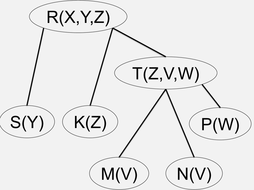
$$A(V) =M(V)\wedge N(V)$$

$$B(Z) =T(Z,V,W)\wedge A(V)\wedge P(W)$$

$$A^{\prime}(Z) =K(Z)\wedge B(Z)$$

$$B^{\prime}(X) =R(X,Y,Z)\wedge S(Y)\wedge A^{\prime}(Z)$$

Figure 4. A tree decomposition for $Q$ in Example 3.5

Algorithm 2 evaluates $Q$ on the worst case instance $W(\Delta\hat{S})$ without materializing $W$. Since the algorithm uses piecewise linear CDS, the computation may lead to rounding errors causing a slight over-approximation of the upper bound in Eq. (5). For that reason, the bound computed by the algorithm is called the Functional Degree Sequence Bound, FDSB. The key observation in the algorithm is that every unary relation $A(X)$ or $B(X_{0})$ is also piecewise constant; for that reason we call them in the algorithm $\hat{f}_{A.X_{0}}(i)$ and $\hat{f}_{B.X}(i)$ respectively. To see this, consider an $\alpha$-step: $A(X)=B_{1}(X)\wedge B_{2}(X)\wedge\cdots$ If each $B_{\ell}$ contains the values $1,2,3,\ldots$, then so will $A$, and the multiplicity of the value $i$ is the product of the multiplicities in the $B_{\ell}$’s: this justifies line 4: $\hat{f}_{A.X}(i)=\hat{f}_{B_{1}.X}(i)*\hat{f}_{B_{2}.X}(i)*\cdots$ The product of piecewise constant functions is still piecewise constant, with a number of segments equal to the sum of all segments of the summands. Consider now a $\beta$-step, Eq. (7). The multiplicity of $i$ in the output $B$ is the product $\hat{f}_{R.X_{0}}(i)*\hat{f}_{A_{1}.X_{1}}(i_{1})*\hat{f}_{A_{2}.X_{2}}(i_{2})*\cdots$, where the ranks $i_{1},i_{2},\ldots$ need to be looked up using the expression $i_{\ell}=\hat{F}_{R.X_{\ell}}^{-1}(\hat{F}_{R.X_{0}}(i))$; this justifies line 9. Here, too, we observe that $i_{\ell}$ is given by a piecewise linear function in $i$, while $\hat{f}_{A_{\ell}.X_{\ell}}(i_{\ell})$ is piecewise constant. In our implementation, both lines 4 and 9 of the algorithm compute a representation of the resulting piecewise constant functions. This representation consists of three vectors; slopes, intercepts, and right interval edges. Because of this representation, multiplication of functions only requires a single pass over these arrays while computing the inverse term, $\hat{F}_{R.X_{\ell}}^{-1}(\hat{F}_{R.X_{0}}(i))$, involves performing a binary search for each of the interior function’s segments. Finally, the algorithm returns the cardinality of the last unary relation at the root. The following theorem from (Deeds et al., 2022) also applies to our setting:

Algorithm 2 Algorithm for $\text{FDSB}(Q,\hat{S})$.

0:  A query plan for $Q$ consisting of $\alpha,\beta$ steps.

1:  for each step do

2:     if $\alpha$-step then

3:        // $A(X)=B_{1}(X)\wedge\ldots\wedge B_{m}(X)$

4:        $\hat{f}_{A.X}(i)=\prod_{\ell=1}^{m}\hat{f}_{B_{\ell}.X}(i)$

5:        // Note: $\hat{f}_{A.X}$ is a piecewise constant function

6:     end if

7:     if $\beta$-step then

8:        // $B(X_{0})=R(X_{0},X_{1},\ldots,X_{k})\wedge A_{1}(X_{1})\wedge\ldots\wedge A_{k}(X_{k})$

9:        $\hat{f}_{B.X_{0}}(i)=\hat{f}_{R.X_{0}}(i)\prod_{\ell=1}^{k}\hat{f}_{A_{\ell}.X_{\ell}}\left(\hat{F}_{R.X_{\ell}}^{-1}(\hat{F}_{R.X_{0}}(i))\right)$

10:        // Note: $\hat{f}_{B.X_{0}}$ is a piecewise constant function

11:     end if

12:  end for

13:  return  $\sum_{i}\hat{f}_{B_{\text{root}}.X}(i)$

Theorem 3.4.

Let $\hat{S}$ consists of piecewise linear CDS, and let $K$ be the total number of segments occurring in all CDS. Then,

1. $|Q(W(\Delta\hat{S}))|\leq\text{FDSB}(Q,\hat{S})$.

2. $\text{FDSB}(Q,\hat{S})$ can be computed in time $O(K\log(K))$.

The first item asserts that FDSB is a correct upper bound. The second item shows that we can compute it in log-linear time relative to the size of the compressed representations. We usually have $10-30$ segments per degree sequence, thus a query with 5 joins has at most $K=300$. This results in very fast inference as shown in Section 5.

3.6. Discussion: More Complex Join Graphs

Cyclic Queries: If $Q$ is a cyclic query, then we compute its upper bound as the minimum of the DSBs of all its spanning trees (which are acyclic). For example, if $Q$ is $R(X,Y)S(Y,Z)T(Z,X)$, there are three spanning trees $R(X,Y)S(Y,Z)$, and $R(X,Y)T(Z,X)$, and $S(Y,Z)T(Z,X)$, and we return the minimum of their DSB.

Multi-Column Joins: We provide two methods of handling multi-column joins. (1) Treat multiple columns as a single column at construction time and calculate its CDS just like for a single column. (2) Alternatively, we note that the CDS for any single column is an upper bound on the CDS of a set of columns. Therefore, we can always upper bound the CDS of the set of columns by taking the minimum of the CDS of each of its columns.

Undeclared Join Columns: We provide a fallback mechanism to handle queries with joins on columns that are not in the declared join column set. During offline construction, we keep a compressed CDS for every column in the relation without conditioning on any predicates. This incurs minimal overhead as it only calculates one CDS per column. At query-time, we calculate a CDS for any declared join column and use it to derive an upper bound on the filtered relation’s cardinality. We then truncate the undeclared join column’s CDS to match this single-table cardinality bound and use this to approximate the filtered CDS of the undeclared join column. This allows us to adapt the bound to the lower cardinality induced by any predicates on the relation. However, the resulting CDS is likely overly skewed because it assumes that the predicate retains precisely the high degree values.

4. Optimizations

Here, we present optimizations that reduce the space consumption and increase the accuracy of the vanilla design.

4.1. Compressing a Set of CDS

To reduce the memory overhead of storing a CDS set for every bin, value, and N-gram, we go beyond compressing a single CDS and consider compressing groups of CDS sets together. Specifically, we divide the CDS sets into groups of ”similar” functions and replace each group with the point-wise maximum of those sets.

To motivate this, we first present a breakdown of the memory cost of SafeBound’s statistics. Let $b$ be the granularity, e.g. the number of buckets in the histogram, and let $k$ be the number of segments in each CDS. Further, let $|V_{J}|$ and $|V_{F}|$ be the number of join and filter columns, respectively. The memory footprint without performing any grouping compression is $O(b|V_{F}|+bk|V_{F}||V_{j}|)$ where the first term is the bucket bounds or values in the MCV list while the second term is the cost of storing the CDS sets. Now, consider dividing the CDS sets into $M$ groups and storing just the maximum over each group. The memory footprint then becomes $O(b|V_{F}|+Mk|V_{F}||V_{j}|)$ which allows us to decouple the granularity of our statistics, $b$, from the accuracy of our approximations, $Mk$. This is crucial for workloads which feature highly selective predicates because it allow us to keep more fine-grained histogram buckets, MCV lists, and N-grams.

As an example, consider a range predicate $.1\leq R.A<.2$. We may only have the memory to store buckets of width $1$ if we store every bucket’s CDS exactly. However, if we cluster and compress our CDS sets with an average cluster size of $10$, we may able to have buckets of width $.1$ which encapsulate the query much tighter while only incurring a $40\%$ relative approximation error. The relative approximation error in this case is far outweighed by the improved granularity of our statistics.

Choosing a Distance Metric: The first step to clustering is choosing a distance metric for the problem. The perfect distance metric for this problem is the average error incurred on the workload when the two functions are replaced with their maximum. However, we don’t have access to the workload when clustering, so we instead use the same assumption that we used in Sec. 3.4, that the workload consists of self-joins. Therefore, our distance metric becomes the self-join error, i.e.

$$d(F_{1},F_{2})=\frac{\sum_{i=1}^{|\mathbb{D}_{V}|}\Delta\max(F_{1}(i),F_{2}(i))^{2}}{\sum_{i=1}^{|\mathbb{D}_{V}|}f_{1}(i)^{2}}+\frac{\sum_{i=1}^{|\mathbb{D}_{V}|}\Delta\max(F_{1}(i),F_{2}(i)^{2}}{\sum_{i=1}^{|\mathbb{D}_{V}|}f_{2}(i)^{2}}$$

.

Choosing a Clustering Algorithm: Given this distance metric, we need to choose a clustering algorithm, and we choose complete-linkage clustering  (Müllner, 2013). This method of hierarchical clustering defines the distance between clusters as the maximum distance between points in each cluster. As opposed to other clustering methods such as single-linkage clustering, it produces tighter clusters and avoids long ”chain” clusters which contain highly dissimilar points. This results in clusters of functions which are well approximated by their point-wise maximums.

4.2. Pre-Computing Primary Key Joins

Predicates Induce Cross-Join Correlation: As described in Section 2.3, the FDSB makes worst-case assumptions about the correlation of columns in joining tables. This assumption is fundamental to computing an upper bound. However, particularly in the presence of predicates, these assumptions may not hold, causing SafeBound to overestimate the query size.

For example, consider the tables MovieKeywords and Keywords from the JOB Benchmark. The former is a fact table with two foreign key columns, MovieId and KeywordId, that associate movies with keywords. The latter is a much smaller dimension table with a primary key column KeywordId and a filter column Keyword, which provides human-readable descriptions of these keywords, e.g. ’character-name-in-title’ or ’pg-13’. A natural query would join them with an equality predicate on the Keyword column to find movies with a particular keyword. A naive version of SafeBound would assume that the selected keyword corresponds to the most frequent value of KeywordId in the MovieKeywords table. If the queried keyword actually occurs infrequently in MovieKeywords, this could introduce a massive error in the final estimation.

Handling Predicate-Induced Correlation: To avoid this issue, SafeBound pre-computes PK-FK joins and stores statistics about the filter columns of the PK relations. In our example, this would mean joining MovieKeywords and Keywords then generating statistics on the resulting keyword column in MovieKeywords. When an equality predicate is applied to the keyword column on the Keywords table, SafeBound applies this predicate to the MovieKeywords table as well, allowing it to directly estimate the CDS set given the predicate without resorting to worst-case assumptions.

Fortunately, the PK-FK join size is bounded by the size of the FK table, so this pre-computation is tractable. While this does not capture all correlations, it does enable accurate estimation for the ubiquitous fact/dimension table design where predicates are applied to dimension tables then propagated to fact tables via PK-FK joins.

4.3. Bloom Filters

An important source of overhead in SafeBound’s data structures are the most common values lists (MCV lists) that it keeps for handling equality predicates. Because values can have an unbounded size, storing a naive MCV list can result in significant memory and lookup overhead. To avoid this overhead, we instead represent our MCV lists as a set of Bloom filters. A Bloom filter is an approximate data structure, which answers the question ”is $x$ an element of the set $S$?” while allowing some false positives and no false negatives. In exchange for approximation, Bloom filters provide a compressed memory footprint ($\approx 12$ bits/value) and fast, constant lookup.

Because Bloom filters only return a positive/negative and SafeBound needs to connect values to their CDS group, we can’t represent the whole MCV list in one filter. Instead, we allocate a filter for each CDS group and insert all values whose CDSs are in that group into its filter. At query time, SafeBound then checks for membership in every group’s filter and takes the maximum over all CDS sets whose filter return positive.

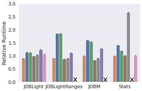
(a) Total workload runtimes relative to runtimes achieved with perfect cardinality estimates. SafeBound results in nearly optimal overall runtimes.

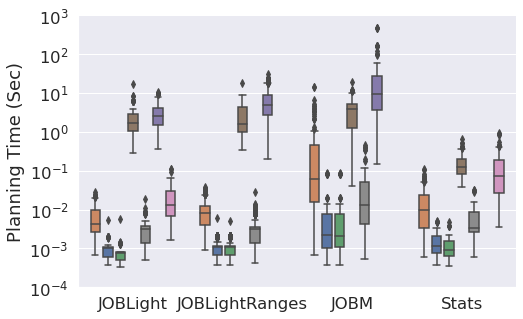
(b) SafeBound achieves 3x-500x faster median planning time than PessEst and ML-based methods across all benchmarks.

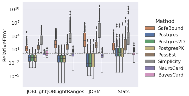
(c) Relative errors for cardinality estimates. SafeBound’s bounds have similar errors to traditional estimates while never underestimating cardinalities.

Figure 5. Workload runtimes, planning time, and estimation error

5. Evaluation

In this section we present an empirical evaluation of SafeBound. We addressed the following questions. How well does SafeBound perform in end-to-end workloads (Sec. 5.1)? How does its memory footprint and inference time compare to existing methods (Sec. 5.2)? How does SafeBound affect DBMS robustness, e.g. performance regressions when new indices are added (Sec. 5.3)? We also conducted several micro-benchmarks in Sec. 5.4, and explored how SafeBound scaled in Sec. 5.5.

Metrics We used the following metrics in our evaluation. (1) Plan Quality (Workload Runtime): Following recent work on benchmarking cardinality estimators (Han et al., 2021) we measure the end-to-end runtime of a query workload in Postgres where we injected alternate cardinality estimators into the optimizer. We run each workload and method five times from a cold cache and present the average relative to the baseline of inserting the true cardinality estimates. (2) Memory Footprint: We compare the size of the stored statistics file on disk, and for Postgres we calculate the size of the pg_statistic and pg_statistic_extended catalog tables. We do not report memory statistics for PessEst as it does not pre-compute statistics. (3) Planning Time: We further consider the planning time for each method. This includes the inference time required to get estimates for every sub-query as well as Postgres’ optimization time given injected estimates. (4) Relative Error: Lastly, we present the relative error of each method as $\text{Error}=(\text{Estimate}/\text{True Cardinality})$. We prefer this metric to $q$-error as it retains information about whether a method overestimates or underestimates.

Datasets We use two datasets, IMDB and Stats. For IMDB we consider three different query workloads from previous work (Yang et al., 2020a; Kipf et al., 2019; Hilprecht et al., 2020): JOB-Light consists of $70$ queries on a subset of $6$ tables in IMDB with $2-5$ PK-FK joins and $1-4$ filter predicates on numeric columns. JOB-LightRanges operates on the same table subset as JOB-Light, but it has $1000$ queries, includes additional columns, and predicates over string columns. And JOB-M is a modified version of the original JOB benchmark; it is the most complex benchmark considered, with 113 queries over 16 tables, and includes significantly more complicated expressions such as IN and LIKE predicates. The Stats dataset is built over a Statistics StackOverflow, and consists of a workload with $146$ queries spanning $8$ tables. While restricted to numeric columns, it has $2-16$ predicates and joins $2-8$ tables per query making it is considered to be a challenging benchmark for cardinality estimation (Han et al., 2021). It has a complicated schema with cyclic primary key/foreign key relationships.

Compared Systems We compared SafeBound against the following systems. (1) Postgres: As a baseline, we compare against the built-in cardinality estimator for Postgres v13. This system uses System-R style estimation combined with years of tuning and carefully chosen magic constants. It stores 1D histograms, most common value lists, and distinct counts for each attribute in a relation. (2) Postgres 2D: We make use of Postgres’ extended statistics, which allows the user to keep statistics on pairs of columns. We instruct the system to store statistics for every pair of filter columns. (3) Postgres PK: SafeBound precomputes statistics on key, foreign-key joins, and so do BayesCard, and NeuroCard; PessEst computes PK-FK joins at query time when needed (Cai et al., 2019, Sec.3.3). To understand the effect of these computations, we measured how much such precomputations could help Postgres. We pre-computed and materialized the PK-FK joins, replaced the FK tables with this join (extending them with additional columns from the PK tables), and computed statistics on these tables. We also adjusted the queries accordingly. For example, consider the query $Q(X,A,B)=R(X,A)S(\underline{A},B,Y)T(\underline{B},Z)\wedge S.Y<10\wedge T.Z>5$ where $S.A$, $T.B$ are PKs. We calculate the PK-FK join results $R^{\prime}(X,A,Y^{\prime})$ and $S^{\prime}(A,B,Y,Z^{\prime})$ and adjust the query to $Q^{\prime}(X,A,B)=R^{\prime}(X,A,Y^{\prime})S^{\prime}(\underline{A},B,Y,Z^{\prime})T(\underline{B},Z)\wedge R^{\prime}.Y^{\prime}<10\wedge S^{\prime}.Z^{\prime}>5$. We call this modifed system PostgresPK. Notice that this mirrors our method by propagating statistics across PK-FK joins, without modifying the query’s join graph.

(4) BayesCard: This is an ML method that uses ensembles of Bayesian Networks trained on subsets of the join schema to produce cardinality estimates (Wu et al., 2020). Recent work has shown that it matches previous ML methods in accuracy while being faster and more compact (Han et al., 2021). (5) NeuroCard: this is an ML method that builds an autoregressive model over a sample of the full outer join of the schema (Yang et al., 2020b). (6) PessEst: The main prior work on cardinality bounding (Cai et al., 2019). It refines a subset of the Polymatroid Bound using a hash partitioning scheme; we use $4096$ hash partitions. However, this method requires scans of the base table to estimate queries with predicates. (7) Simplicity: a cardinality estimator which uses single-table cardinalities and max degrees of join columns (Hertzschuch et al., 2021). In order to improve the max degree in the presence of predicates, Simplicity relies on samples (Hertzschuch et al., 2021) or on estimates derived from Postgres, which are no longer leading to guaranteed upper bounds. In the original prototype and our implementation, the single-table estimates are derived from Postgres although more complicated sampling mechanisms are proposed in the paper. Similarly, we do not consider their greedy join ordering algorithm, instead focusing solely on the cardinality estimator.

Experimental Setup In our experiments, we use an instance of Postgres v13 and input cardinality estimates using the pg_hint_plan extension. We adjust the default settings of Postgres per the recommendation of  (Leis et al., 2018) setting the shared memory to 4GB, worker memory to 2GB, implicit OS cache size to 32 GB, and max parallel workers to 6. Additionally, we enable indices on primary and foreign keys. We run all experiments on an AWS EC2 instance (m5.8xlarge) with 32 vCPUs and 128 GB of memory.

Figure 6. The runtime of the 80 longest-running queries across all benchmarks. Estimates from SafeBound result in faster query execution on the most expensive queries with a p05/p25/p50/p75/p95 quantile speedup of 1.01x/1.3x/1.7x/10.1x/30.3x.

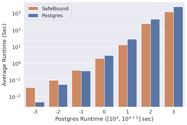
Figure 7. The average runtime of queries binned by their runtime using Postgres’ estimates. SafeBound outperforms Postgres’ estimates for queries with runtime over one second.

5.1. End-to-End Performance

Nearly optimal workload runtimes across all benchmarks. We show the workload runtimes across a variety of benchmarks and cardinality estimation methods in Figure 5(a). Across all four benchmarks, plans generated using SafeBound’s estimates achieve workload runtimes equivalent to those generated with the true cardinalities. As found in previous work, using true cardinality does not always lead to optimal plans due to imperfect cost modeling (Han et al., 2021). SafeBound achieves $20\%-85\%$ lower runtimes than Postgres on all benchmarks. BayesCard and PessEst perform similarly to SafeBound on all benchmarks while NeuroCard has $20-30\%$ worse performance on both JOBLight and JOBM. Bayescard does not support the string predicates of JOB-LightRanges or JOB-M, and NeuroCard does not support the cyclic schema of the Stats benchmark. All pessimistic systems achieve good performance on the JOB benchmarks, pointing to the utility of even fairly loose cardinality bounds. However, Simplicity results in a poor join ordering for query 132 of the Stats benchmark, resulting in a 1500x slowdown.

Efficient plans for the queries that matter. To provide context for SafeBound’s performance, we examine the runtime of the longest running queries in Figure 6. The queries that make up the bulk of the runtime can often be sped up significantly (up to $60x$) by using SafeBound instead of Postgres for cardinality estimates.

Figure 7 buckets the queries across all workloads by runtime and shows the average runtime using SafeBound and Postgres’s estimates. Here, we can see SafeBound generally achieves a significant speedup for queries that take over a second. We see these speedups because cardinality bounds encourage the query optimizer to make conservative decisions (e.g. choosing hash joins over nested loop joins) which tend to be the correct decisions for queries with long runtimes or large outputs. For the fastest queries, SafeBound often results in slower execution as it discourages the optimizer from choosing high-risk high-reward plans.

Estimation Errors. In Figure 5(c), we show the relative estimation error on full queries for each of the benchmarks and methods. SafeBound has a similar range of errors as Postgres, but guarantees that it never underestimates: its estimates in the figure always lie above the center line. Traditional estimators frequently underestimate by $10^{3}$ or more which is detrimental to query optimization. Notably, additional optimisations such as Postgres2D and PostgresPK do not significantly alter the estimates. This implies that the errors primarily stem from the fundamental independence assumptions rather than a lack of statistics. ML-based methods produce accurate estimates, but still lack guarantees; NeuroCard is prone to significant underestimates. The Simplicity system overestimates significantly due to its reliance on the max degree without conditioning on predicates. Moreover, as discussed, its “upper bound” is not guaranteed: it returns a wrong upper bound on two of the queries of JOBLightRanges. Because it handles predicates by scanning the table at estimation time, PessEst has good estimates for queries with many predicates or with challenging predicates such as JOB-LightRanges and JOB-M. We provide a more detailed breakdown of estimation error by number of tables in the appendix.

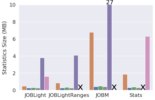
(a) Across all benchmarks, SafeBound uses 3x-6.8x less space than ML methods.

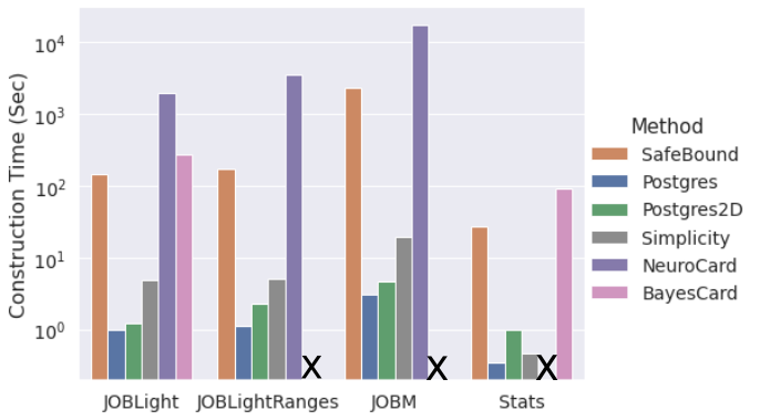
(b) SafeBound achieves up to 17x lower offline statistics construction time than ML methods.

Figure 8. Statistic Size and Construction Time

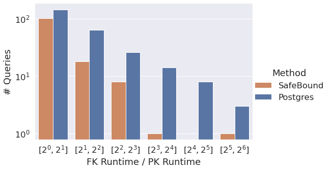
(a) The frequency and magnitude of FK index performance regressions. SafeBounds estimates result in fewer and less severe regressions.

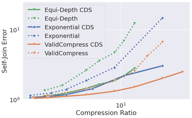
(b) Modeling the CDS results in lower error than modeling the DS, and our two-pass algorithm outperforms heuristic methods.

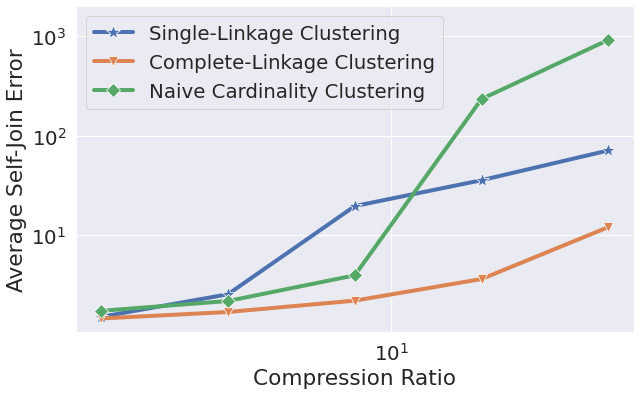
(c) Complete-linkage clustering of CDS produces low error even at high compression rates.

Figure 9. Micro-Benchmarks and Performance Regression Study

5.2. Planning Time, Memory, and Build Time

Figure 5(b) reports the planning times (Postgres’ optimization and the cost estimation time for all sub-queries) for all systems and benchmarks. Postgres’ efficient C implementation and use of dynamic programming in estimating sub-queries results in the fastest planning time. The Simplicity system achieves good planning times thanks to its straightforward bound calculation and reliance on Postgres’s fast single-table estimates. PessEst requires scanning the base tables at runtime when predicates are applied, resulting in 12x-420x slower inference. The ML methods, particularly Neurocard, perform inference on complex black-box models which leads to poor inference latency. SafeBound implements Algorithm 13, which runs in log-linear time in the size of the compressed degree sequences. This results in much faster planning times than PessEst, BayesCard, and NeuroCard across all benchmarks.

Next, we turn to the memory footprint, which we report in Figure 8(a). Safebound’s simple statistics and compression techniques allow it to achieve a compact memory footprint close to traditional methods like Postgres. For instance, group compression results in 7.3-43x fewer degree sequences being stored across benchmarks. This results in statistics that are only 200KB larger than Postgres’ for the JOB-Light benchmark and over 3x smaller for all benchmarks than BayesCard and NeuroCard which rely on complex black box models. Simplicity relies on the statistics stored in Postgres and the max degree of each join column, resulting in a small memory footprint. PessEst does not operate on pre-computed statistics, so its space and build time is not reported.

Finally, we considered the build time. SafeBound has 2-3.5x and 8-20x faster build time than BayesCard and NeuroCard, respectively. We note that SafeBound’s build process (Algorithm 1) is a series of aggregations over the base data to create histograms and MCV lists, resulting in relatively fast construction despite building from the full dataset rather than a sample. Traditional estimators remain the fastest as they perform similar aggregations to SafeBound but on a small sample of the data. The string predicates of JOB-M result in longer build times for SafeBound and NeuroCard because they require the calculation of tri-grams and factorized columns, respectively. Postgres(2D), on the other hand, does not keep statistics for LIKE predicates (instead handling them via a magic constant), so the additional complexity does not affect their time.

5.3. Robustness Against Regressions

When attempting to tune database instances, users often face inexplicable performance regressions. Creating an index on a join column is reasonably assumed by users to improve query performance, but will frequently cause queries to run significantly slower. This is primarily due to the query optimizer receiving cardinality underestimates and optimistically making use of the index for a query where a hash or merge join is faster. In figure 9(a), we show the frequency and severity of regressions across all benchmarks when Postgres’ internal estimates are used vs SafeBounds cardinality bounds. While some regressions still occur due to issues in cost modeling, SafeBound produces half as many performance regressions across all benchmarks, $129$ to Postgres’ $259$, and they are half as severe on average, $1.7$x to Postgres’ $3.3$x.

5.4. Micro-Benchmarks

In the following experiments, we evaluate how SafeBound’s components perform individually as compared to alternatives. To do this, we calculate the error on self-join queries with equality predicates, specifically the MovieCompanies relation joining with itself on MovieId with and without an equality predicate on ProductionYear.

Modeling the CDS rather than the DS reduces error by up to 20x. By avoiding artificial inflation of the relations’ cardinality caused by modeling the DS directly, SafeBound achieves significantly more accurate estimates. This can be seen on Figure 9(b) which shows the accuracy of various approximation methods for modeling the full CDS/DS of MovieCompanies.MovieId versus the compression ratio (# distinct frequencies/ # segments). The different colors correspond to different ways of choosing the segment boundaries for the approximation while the solid vs dashed lines correspond to whether the method models the CDS or the DS, respectively. As we would expect, every approximation method has lower error when applied to the CDS rather than the DS.

The ValidApprox algorithm efficiently models the CDS. Looking again at Figure 9(b), we can compare the solid lines to get a sense for how different segmentation strategies affect the accuracy/compression trade-off. We compare against a couple of reasonable baselines, 1) an equi-depth strategy which segments the degree sequence into equal-cardinality segments 2) an exponential strategy which uses a geometric sequence for segment boundaries. Our two-pass algorithms outperform both baselines because it adjusts the size of buckets based on the skewness of the underlying degree sequence, taking into account both the importance of high frequency items and the long tail of the distribution.

Complete-linkage clustering of CDSs provides low error at high compression ratios. The experiment in Figure 9(c) shows the effect of different clustering techniques. In this experiment, we joined the MovieCompanies relation with the Title relation according to their FK/PK relationship then calculate an MCV list for the ProductionYear attribute as described in Sec. 3.2. This results in $132$ CDS that we use to test various clustering methods, which cluster them into between $4$ and $64$ groups, and we represent each cluster with the maximum as in Sec. 4.1. The error metric is then the average relative self-join error over all the original CDS when they are approximated using their cluster’s maximum. In this case, compression ratio is defined as the number of original groups, $132$, divided by the number of clusters after compression.

We compare SafeBound’s method, complete-linkage clustering, with single-linkage clustering and the naive method of grouping the functions into equal sized clusters by cardinality. Across these methods, complete-linkage clustering results in lower error for all compression ratios. This is because naive clustering doesn’t take into account the shape of the CDS and doesn’t adaptively choose cluster sizes, and single-linkage clustering often produces long chaining clusters where one CDS dominates the maximum.

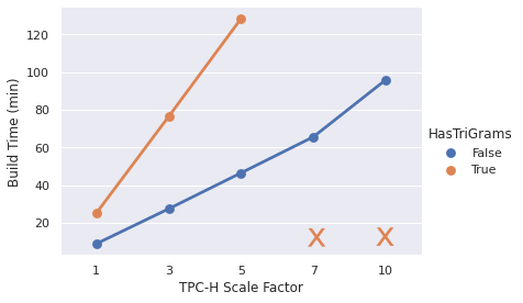
Figure 10. The pre-processing overhead increases linearly with the size of the dataset. [Python Prototype]

5.5. Scalability

To test how SafeBound scales to both more complex schemas and larger datasets, we experiment with the TPC-H benchmark at various scaling factors in Fig 10. This benchmark has 14 join columns, 46 filter columns, and 9 PK-FK relationships over 8 tables, and we vary the scale factor from 1GB to 10GB. We further build two versions of SafeBound: one where it constructs tri-gram statistics for LIKE predicates and one where it does not. This experiment shows that the construction time increases linearly in the size of the data. However, it also points to the inefficiency of the current python implementation in two ways. It runs out of memory when computing tri-grams for higher scale factors (as denoted by the X marks), and the build process is slower than expected given the simple underlying operations. This is in line with recent research which has shown an average of 29x worse performance when using CPython rather than C++ for a variety of applications due to dynamic type checking, interpreter overhead, and the global interpreter lock (Lion et al., 2022).

6. Limitations and Future Work

This work represents SafeBound, a first practical system for computing guaranteed cardinality upper bounds: previous upper bound systems either require significant query time computation (PessEst), or do not provide guaranteed bounds (Simplicity). SafeBound achieves up to 80% lower end-to-end runtimes than PostgreSQL across workloads, and is on par or better than state of the art ML-based estimators and pessimistic cardinality estimators. Yet, the current SafeBound prototype is likely not yet ready for a production system, due to a few limitations, which we discuss here.

Build Time: Any upper bound system must, at some point, read all rows in the database. This places a hard lower bound on the build time for cardinality bounding systems. Therefore, future work to reduce this expense will need to exploit parallelism or take advantage of times when the system is already scanning the data (e.g. during bulk loading or query execution).

Handling Updates: A challenge that we leave open is handling updates without recomputing the degree sequences. We note here that a degree sequences is essentially a group-by/count/order-by query and could benefit from IVM techniques (Koch et al., 2014).

Multiple Predicates Per Table: SafeBound handles the existence of multiple predicates on a single relation by taking the minimum of their induced CDS’. However, this results in an estimated cardinality equal to the selectivity of the most selective predicate. This could be inaccurate when faced with multiple moderately selective predicates which are jointly highly selective. Future work should consider ways of keeping lightweight statistics on combinations of filter columns in order to tackle this problem.

Correctness and Accuracy: SafeBound does not rely on any statistical assumptions about the data for correctness: it always provides a correct upper bound, regardless of the underlying data distribution, even in the presence of predicates. However, Sec. 3 describes heuristics which affect the space/accuracy tradeoff, and queries which do not conform to the assumptions may see poor performance (e.g. joins on tables with very different skews or highly selective predicates). Further, like nearly all non-sampling methods, SafeBound does not provide a precise characterization of its error. Improving these heurstics or formally characterizing the tightness of SafeBound is an exciting avenue for future work.

References

- (1)
- Anonymized authors for double blind reviewing (2022) Anonymized authors for double blind reviewing. 2022. Online Appendix. https://github.com/AnonymousSigmod2023/SafeBound
- Cai et al. (2019) Walter Cai, Magdalena Balazinska, and Dan Suciu. 2019. Pessimistic Cardinality Estimation: Tighter Upper Bounds for Intermediate Join Cardinalities. In Proceedings of the 2019 International Conference on Management of Data, SIGMOD Conference 2019, Amsterdam, The Netherlands, June 30 - July 5, 2019, Peter A. Boncz, Stefan Manegold, Anastasia Ailamaki, Amol Deshpande, and Tim Kraska (Eds.). ACM, 18–35. https://doi.org/10.1145/3299869.3319894
- Chen et al. (2022) Jeremy Chen, Yuqing Huang, Mushi Wang, Semih Salihoglu, and Kenneth Salem. 2022. Accurate Summary-based Cardinality Estimation Through the Lens of Cardinality Estimation Graphs. Proc. VLDB Endow. 15, 8 (2022), 1533–1545. https://www.vldb.org/pvldb/vol15/p1533-chen.pdf
- Deeds et al. (2022) Kyle Deeds, Dan Suciu, Magda Balazinska, and Walter Cai. 2022. Degree Sequence Bound For Join Cardinality Estimation. CoRR abs/2201.04166 (2022). arXiv:2201.04166 https://arxiv.org/abs/2201.04166
- Fagin (1983) Ronald Fagin. 1983. Degrees of acyclicity for hypergraphs and relational database schemes. Journal of the ACM (JACM) 30, 3 (1983), 514–550.
- Ferragina and Vinciguerra (2020) Paolo Ferragina and Giorgio Vinciguerra. 2020. The PGM-index: a fully-dynamic compressed learned index with provable worst-case bounds. Proceedings of the VLDB Endowment 13, 8 (2020), 1162–1175.
- Gottlob et al. (2012) Georg Gottlob, Stephanie Tien Lee, Gregory Valiant, and Paul Valiant. 2012. Size and Treewidth Bounds for Conjunctive Queries. J. ACM 59, 3 (2012), 16:1–16:35. https://doi.org/10.1145/2220357.2220363
- Grohe and Marx (2006) Martin Grohe and Dániel Marx. 2006. Constraint solving via fractional edge covers. In Proceedings of the Seventeenth Annual ACM-SIAM Symposium on Discrete Algorithms, SODA 2006, Miami, Florida, USA, January 22-26, 2006. ACM Press, 289–298. http://dl.acm.org/citation.cfm?id=1109557.1109590
- Han et al. (2021) Yuxing Han, Ziniu Wu, Peizhi Wu, Rong Zhu, Jingyi Yang, Liang Wei Tan, Kai Zeng, Gao Cong, Yanzhao Qin, Andreas Pfadler, Zhengping Qian, Jingren Zhou, Jiangneng Li, and Bin Cui. 2021. Cardinality Estimation in DBMS: A Comprehensive Benchmark Evaluation. Proc. VLDB Endow. 15, 4 (2021), 752–765. https://doi.org/10.14778/3503585.3503586
- Hertzschuch et al. (2021) Axel Hertzschuch, Claudio Hartmann, Dirk Habich, and Wolfgang Lehner. 2021. Simplicity Done Right for Join Ordering. In 11th Conference on Innovative Data Systems Research, CIDR 2021, Virtual Event, January 11-15, 2021, Online Proceedings. www.cidrdb.org. http://cidrdb.org/cidr2021/papers/cidr2021_paper01.pdf
- Hilprecht et al. (2020) Benjamin Hilprecht, Andreas Schmidt, Moritz Kulessa, Alejandro Molina, Kristian Kersting, and Carsten Binnig. 2020. DeepDB: Learn from Data, not from Queries! Proc. VLDB Endow. 13, 7 (2020), 992–1005. https://doi.org/10.14778/3384345.3384349
- Khamis et al. (2016) Mahmoud Abo Khamis, Hung Q. Ngo, and Dan Suciu. 2016. Computing Join Queries with Functional Dependencies. In Proceedings of the 35th ACM SIGMOD-SIGACT-SIGAI Symposium on Principles of Database Systems, PODS 2016, San Francisco, CA, USA, June 26 - July 01, 2016, Tova Milo and Wang-Chiew Tan (Eds.). ACM, 327–342. https://doi.org/10.1145/2902251.2902289
- Khamis et al. (2017) Mahmoud Abo Khamis, Hung Q. Ngo, and Dan Suciu. 2017. What Do Shannon-type Inequalities, Submodular Width, and Disjunctive Datalog Have to Do with One Another?. In Proceedings of the 36th ACM SIGMOD-SIGACT-SIGAI Symposium on Principles of Database Systems, PODS 2017, Chicago, IL, USA, May 14-19, 2017, Emanuel Sallinger, Jan Van den Bussche, and Floris Geerts (Eds.). ACM, 429–444. https://doi.org/10.1145/3034786.3056105
- Kim et al. (2022) Kyoungmin Kim, Jisung Jung, In Seo, Wook-Shin Han, Kangwoo Choi, and Jaehyok Chong. 2022. Learned Cardinality Estimation: An In-depth Study. In SIGMOD ’22: International Conference on Management of Data, Philadelphia, PA, USA, June 12 - 17, 2022, Zachary Ives, Angela Bonifati, and Amr El Abbadi (Eds.). ACM, 1214–1227. https://doi.org/10.1145/3514221.3526154
- Kipf et al. (2019) Andreas Kipf, Thomas Kipf, Bernhard Radke, Viktor Leis, Peter A. Boncz, and Alfons Kemper. 2019. Learned Cardinalities: Estimating Correlated Joins with Deep Learning. In 9th Biennial Conference on Innovative Data Systems Research, CIDR 2019, Asilomar, CA, USA, January 13-16, 2019, Online Proceedings. www.cidrdb.org. http://cidrdb.org/cidr2019/papers/p101-kipf-cidr19.pdf
- Koch et al. (2014) Christoph Koch, Yanif Ahmad, Oliver Kennedy, Milos Nikolic, Andres Nötzli, Daniel Lupei, and Amir Shaikhha. 2014. DBToaster: higher-order delta processing for dynamic, frequently fresh views. VLDB J. 23, 2 (2014), 253–278. https://doi.org/10.1007/s00778-013-0348-4
- Leis et al. (2018) Viktor Leis, Bernhard Radke, Andrey Gubichev, Atanas Mirchev, Peter A. Boncz, Alfons Kemper, and Thomas Neumann. 2018. Query optimization through the looking glass, and what we found running the Join Order Benchmark. VLDB J. 27, 5 (2018), 643–668. https://doi.org/10.1007/s00778-017-0480-7
- Lion et al. (2022) David Lion, Adrian Chiu, Michael Stumm, and Ding Yuan. 2022. Investigating Managed Language Runtime Performance: Why JavaScript and Python are 8x and 29x slower than C++, yet Java and Go can be Faster?. In 2022 USENIX Annual Technical Conference (USENIX ATC 22). 835–852.
- Liu et al. (2021) Jie Liu, Wenqian Dong, Dong Li, and Qingqing Zhou. 2021. Fauce: Fast and Accurate Deep Ensembles with Uncertainty for Cardinality Estimation. Proc. VLDB Endow. 14, 11 (2021), 1950–1963. https://doi.org/10.14778/3476249.3476254
- Müllner (2013) Daniel Müllner. 2013. fastcluster: Fast hierarchical, agglomerative clustering routines for R and Python. Journal of Statistical Software 53 (2013), 1–18.
- Negi et al. (2021) Parimarjan Negi, Ryan C. Marcus, Andreas Kipf, Hongzi Mao, Nesime Tatbul, Tim Kraska, and Mohammad Alizadeh. 2021. Flow-Loss: Learning Cardinality Estimates That Matter. Proc. VLDB Endow. 14, 11 (2021), 2019–2032. http://www.vldb.org/pvldb/vol14/p2019-negi.pdf
- Wang et al. (2021a) Jiayi Wang, Chengliang Chai, Jiabin Liu, and Guoliang Li. 2021a. FACE: A Normalizing Flow based Cardinality Estimator. Proc. VLDB Endow. 15, 1 (2021), 72–84. https://doi.org/10.14778/3485450.3485458
- Wang et al. (2021b) Xiaoying Wang, Changbo Qu, Weiyuan Wu, Jiannan Wang, and Qingqing Zhou. 2021b. Are We Ready For Learned Cardinality Estimation? Proc. VLDB Endow. 14, 9 (2021), 1640–1654. https://doi.org/10.14778/3461535.3461552
- Woltmann et al. (2020) Lucas Woltmann, Claudio Hartmann, Dirk Habich, and Wolfgang Lehner. 2020. Best of both worlds: combining traditional and machine learning models for cardinality estimation. In Proceedings of the Third International Workshop on Exploiting Artificial Intelligence Techniques for Data Management, aiDM@SIGMOD 2020, Portland, Oregon, USA, June 19, 2020, Rajesh Bordawekar, Oded Shmueli, Nesime Tatbul, and Tin Kam Ho (Eds.). ACM, 4:1–4:8. https://doi.org/10.1145/3401071.3401658
- Woltmann et al. (2019) Lucas Woltmann, Claudio Hartmann, Maik Thiele, Dirk Habich, and Wolfgang Lehner. 2019. Cardinality estimation with local deep learning models. In Proceedings of the Second International Workshop on Exploiting Artificial Intelligence Techniques for Data Management, aiDM@SIGMOD 2019, Amsterdam, The Netherlands, July 5, 2019, Rajesh Bordawekar and Oded Shmueli (Eds.). ACM, 5:1–5:8. https://doi.org/10.1145/3329859.3329875
- Wu and Cong (2021) Peizhi Wu and Gao Cong. 2021. A Unified Deep Model of Learning from both Data and Queries for Cardinality Estimation. In SIGMOD ’21: International Conference on Management of Data, Virtual Event, China, June 20-25, 2021, Guoliang Li, Zhanhuai Li, Stratos Idreos, and Divesh Srivastava (Eds.). ACM, 2009–2022. https://doi.org/10.1145/3448016.3452830
- Wu et al. (2020) Ziniu Wu, Amir Shaikhha, Rong Zhu, Kai Zeng, Yuxing Han, and Jingren Zhou. 2020. BayesCard: Revitilizing Bayesian Frameworks for Cardinality Estimation. arXiv preprint arXiv:2012.14743 (2020).
- Yang et al. (2020a) Zongheng Yang, Amog Kamsetty, Sifei Luan, Eric Liang, Yan Duan, Xi Chen, and Ion Stoica. 2020a. NeuroCard: One Cardinality Estimator for All Tables. Proc. VLDB Endow. 14, 1 (2020), 61–73. https://doi.org/10.14778/3421424.3421432
- Yang et al. (2020b) Zongheng Yang, Amog Kamsetty, Sifei Luan, Eric Liang, Yan Duan, Xi Chen, and Ion Stoica. 2020b. NeuroCard: one cardinality estimator for all tables. arXiv preprint arXiv:2006.08109 (2020).
- Zhu et al. (2021) Rong Zhu, Ziniu Wu, Yuxing Han, Kai Zeng, Andreas Pfadler, Zhengping Qian, Jingren Zhou, and Bin Cui. 2021. FLAT: Fast, Lightweight and Accurate Method for Cardinality Estimation. Proc. VLDB Endow. 14, 9 (2021), 1489–1502. https://doi.org/10.14778/3461535.3461539