Closed-form analytic expressions for shadow estimation with brickwork circuits

Abstract

Properties of quantum systems can be estimated using classical shadows, which implement measurements based on random ensembles of unitaries. Originally derived for global Clifford unitaries and products of single-qubit Clifford gates, practical implementations are limited to the latter scheme for moderate numbers of qubits. Beyond local gates, the accurate implementation of very short random circuits with two-local gates is still experimentally feasible and, therefore, interesting for implementing measurements in near-term applications. In this work, we derive closed-form analytical expressions for shadow estimation using brickwork circuits with two layers of parallel two-local Haar-random (or Clifford) unitaries. Besides the construction of the classical shadow, our results give rise to sample-complexity guarantees for estimating Pauli observables. We then compare the performance of shadow estimation with brickwork circuits to the established approach using local Clifford unitaries and find improved sample complexity in the estimation of observables supported on sufficiently many qubits.

1 Introduction

Retrieving information about the state of a quantum system is a long-standing problem in quantum information processing and of central practical importance in quantum technologies. Full quantum state tomography can recover a complete, precise classical description of the state but requires a large number of state copies [Kliesch2020TheoryOfQuantum, darianoQuantumTomography2003, DonWri15, HaaHarJi15, FlaGroLiu12], making the protocol feasible only for a very moderate number of qubits. Nevertheless, for many concrete tasks, complete knowledge of the quantum state is often unnecessary [Aaronson2018ShadowTomography], and estimation schemes for specific properties are often scalable.

A particularly attractive estimation primitive is nowadays referred to as shadow estimation [huangPredictingManyProperties2020, painiApproximateDescriptionQuantum2019]. Here, an approximation of a repeatedly prepared unknown quantum state, the so-called classical shadow, is constructed from measurements in randomly selected bases. In the limit of many bases, this approach allows, in principle, for full state tomography. For this reason, classical shadows can be further post-processed to construct estimators for the expectation value of arbitrary sets of observables. Importantly, for certain random measurement ensembles, rigorous analytical guarantees ensure that precise estimates of expectation values can be evaluated long before one has collected enough measurement statistics for full quantum state tomography.

The original examples with strict guarantees on the sample complexity are, in a sense, two “extreme” scenarios: The first one is characterized by evolving the state with a global random Clifford unitary before performing a basis measurement. It is particularly suited for predicting global properties; for instance, fidelity estimation requires a constant number of samples with this setting. The second scheme is built on local Clifford unitaries and effectively amounts to perform measurements in random local Pauli bases. In this case, local properties can often be efficiently estimated [elbenMixedstateEntanglementLocal2020, zhang2021ExperimentalQuantumState, struchalinExperimentalEstimationQuantum2021]. Moreover, biasing the distribution of local Clifford unitaries to the estimation task at hand can yield further improvements in sample complexity [hadfieldMeasurementsQuantumHamiltonians2022].

An accurate estimation requires a precise experimental implementation of the random unitaries. Although more robust variants of shadow estimation exist [chenRobustShadowEstimation2021, kohClassicalShadowsNoise2020], the implementation of global multi-qubit Clifford unitaries on near-term hardware will typically introduce too much noise to be useful for estimation.

Experimentally feasible alternatives, naturally interpolating between the two extreme cases and potentially lowering the sample complexity over local Clifford unitaries, are short Clifford circuits [hu2021ClassicalShadowTomography]. However, finding expressions for classical shadows for random low-depth Clifford circuits is a challenging task. For instance, the construction by hu2021ClassicalShadowTomography involve numerically solving a large system of equations.

In this work, we derive closed-form analytic expressions for the arguably simplest non-trivial circuit construction of classical shadows: One round of a brickwork circuit consisting of two layers of products of random unitaries. Besides providing a more direct construction of the classical shadow, these analytic expressions allow us to compare the sample complexity of the circuit construction to the one with local Clifford unitaries. In particular, we first observe that for Pauli observables, one shall look at pairs of adjacent qubits in the support of such observables and their relative position in the circuit. Then, we find that the (very short) brickwork shadows outperform the local Clifford ones for Pauli observables supported on sufficiently many qubits of a brickwork circuit. Conversely, we also observe that local Clifford unitaries yield a lower sample complexity in the case of Pauli observables supported on sparsely distributed qubits in the sense of the brickwork circuit.

The remainder is structured as follows: Following the observation that the associated measurement channel can be interpreted as a frame (super-)operator [Helsen21EstimatingGate-set] in Section 2.2, we work out its matrix representation in the Pauli basis in Section 3. In particular, using well-known expressions for the second-moment operator of sufficiently uniform probability measures over the unitary group, we derive recurrence relations for subcircuits that can be analytically solved. In LABEL:sec:discussion, we identify the regime where the resulting sample complexity outperforms the shadow estimation protocol with the local Cliffords ensemble, and in LABEL:sec:numerics we compare numerically the performance of brickwork and local Cliffords shadows.

Related works.

During the completion of this work, two other papers on brickwork circuits were published [Akhtar2023scalableflexible, bertoniShallowShadowsExpectation2022]. Both describe shadows associated with brickwork circuits of arbitrary depth and numerically study the measurement channels associated with such circuits using tensor network techniques. In particular, Akhtar2023scalableflexible apply the formalism based on entanglement features introduced by buClassicalShadowsPauliinvariant2022 and discusses average case scenario upper bounds on sample complexity based on the locally scrambled shadow norm [hu2021ClassicalShadowTomography]. A similar discussion, following a probabilistic interpretation of the eigenvalues of the measurement channels, is done by bertoniShallowShadowsExpectation2022. In particular, they provide rigorous upper bounds to the locally scrambled shadow norm for circuits of depth logarithmic in the number of qubits, and find upper bounds to the shadow norm for a class of observables beyond the Pauli case. In comparison, we only focus on single-round brick-layer circuits but provide analytic expressions for the estimator of Pauli observables.

2 Preliminaries

2.1 Notation

We denote the Hilbert-Schmidt inner product by a braket-like notation, namely

$$\operatorname{Tr}(A^{\dagger}B)\equiv(A\kern 0.6458pt|\kern 0.6458pt\mathopen{}B)\quad A,B\in\mathbb{C}^{d\times d}\,.$$ (1)

Likewise, the outer product $|A\kern 0.6458pt)(\kern 0.6458pt\mathopen{}B|$ denotes the superoperator $C\mapsto(B\kern 0.6458pt|\kern 0.6458pt\mathopen{}C)A$. We parametrize single-qubit Pauli operators by binary vectors $v=(z,x)\in\mathbb{F}_{2}^{2}$ as

$$W(0,0) \coloneqq\mathds{1}, W(0,1) \coloneqq X, W(1,0) \coloneqq Z, W(1,1) \coloneqq Y,$$ (2)

where $X,Y,Z\in\mathbb{C}^{2\times 2}$ are the usual Pauli matrices. Then, we define the $n$-qubit Pauli operators as tensor products of the single-qubit Pauli operators, indexed by vectors $v=v_{1}\oplus\dots\oplus v_{n}\in\mathbb{F}_{2}^{2n}$:

$$W(v)\coloneqq W(v_{1})\otimes\dots\otimes W(v_{n})\,.$$ (3)

For a given vector $v=v_{1}\oplus\dots\oplus v_{n}\in\mathbb{F}_{2}^{2n}$, we define its weight vector as the binary vector $\operatorname{wt}(v)\in\mathbb{F}_{2}^{n}$ such that $\operatorname{wt}(v)_{i}=0$ if $v_{i}=(0,0)$ and $\operatorname{wt}(v)_{i}=1$ else. In other words, $\operatorname{wt}(v)$ has a zero in the $i$th position if and only if $W(v)$ is the identity on the $i$th qubit. We use the shorthand notation

$$|v)\equiv\frac{1}{\sqrt{d}}W(v)$$ (4)

for the normalized Pauli operators. Hence, the set $\{|v)\}$ denotes the orthonormal Pauli basis in $\mathbb{C}^{d\times d}$, where $d=2^{n}$ denotes the dimension of the Hilbert space of $n$ qubits from now on.

Finally, for any $k\in\mathbb{N}$, we set $[k]\coloneqq\{1,\dots,k\}$.

2.2 Classical shadows formalism

In this section, we review the shadow estimation protocol [huangPredictingManyProperties2020] in the language of frame theory (see Ref. [waldronIntroductionFiniteTight2018] for an introduction to frame theory). The procedure works as follows: draw unitaries $U\sim\nu$ according to some probability measure $\nu$ on the unitary group $\operatorname{U}(d)$, apply $U$ to the (unknown) state $\rho$, and finally measure in the computational basis $\{E_{i}\coloneqq|i\kern 0.6458pt\rangle\langle\kern 0.6458pt\mathopen{}i|\}_{i\in[d]}$. Having obtained outcome $i$, store the classical snapshot $(i,U)$. Repeating this primitive yields multiple snapshots $\{i_{k},U_{k}\}_{k=1}^{m}$. Finally, given an observable $O$, one evaluates a scalar function $f_{O}(i,U)$ for each snapshot and takes the empirical average $\hat{o}=\sum_{k=1}^{m}f_{O}(i_{k},U_{k})$.

Constructing $f_{O}(i,U)$ as follows ensures that $\hat{o}$ is an unbiased estimator for the expectation value $\operatorname{Tr}(O\rho)$: First, one shall require that $\{E_{i,U}\coloneqq U^{\dagger}E_{i}U\}$ is a tomographically complete, POVM (POVM) [acharya2021ShadowTomographybased], i.e. for all states $\rho\neq\sigma$ there exists a pair $(i,U)$ such that $\langle i\,|\kern 0.6458pt\mathopen{}U\rho U^{\dagger}\kern 0.6458pt|\kern 0.6458pt\mathopen{}i\rangle\neq\langle i\,|\kern 0.6458pt\mathopen{}U\sigma U^{\dagger}\kern 0.6458pt|\kern 0.6458pt\mathopen{}i\rangle$. This ensures that $\{E_{i,U}\}$ is a frame [Moran2013, Kliesch2020TheoryOfQuantum], and the associated measurement channel

$$S(\rho)\coloneqq\sum_{i\in[d]}\mathbb{E}_{U\sim\nu}|E_{i,U})(E_{i,U}\kern 0.6458pt|\kern 0.6458pt\mathopen{}\rho)=\sum_{i\in[d]}\mathbb{E}_{U\sim\nu}\langle i\,|\kern 0.6458pt\mathopen{}U\rho U^{\dagger}\kern 0.6458pt|\kern 0.6458pt\mathopen{}i\rangle\,U^{\dagger}|i\kern 0.6458pt\rangle\langle\kern 0.6458pt\mathopen{}i|U\,$$ (5)

has the interpretation as a frame operator. In particular, $S$ is positive definite, and thus invertible. Then, $\{\tilde{E}_{i,U}\coloneqq S^{-1}(E_{i,U})\}$ is the so-called canonical dual frame, and we have the following relation

$$\operatorname{Tr}(O\rho)=\operatorname{Tr}(OS^{-1}S(\rho))=\sum_{i}\mathbb{E}_{U\sim\nu}(O\kern 0.6458pt|\kern 0.6458pt\mathopen{}\tilde{E}_{i,U})(E_{i,U}\kern 0.6458pt|\kern 0.6458pt\mathopen{}\rho)\,.$$ (6)

Therefore, the last expression can be interpreted as the expected value of $f_{O}(i,U)\coloneqq(O\kern 0.6458pt|\kern 0.6458pt\mathopen{}\tilde{E}_{i,U})$ when sampling $U\sim\nu$ and $i\sim(E_{i,U}\kern 0.6458pt|\kern 0.6458pt\mathopen{}\rho)$ and is, thus, the limit of the empirical average over many experimental snapshots.

However, the computation of the canonical dual frame is in general a highly non-trivial task. Analytical inversion of $S$ is often only possible in special cases where the probability measure $\nu$ is very structured. For instance, if $\nu$ is the Haar measure on $\operatorname{U}(d)$, or a unitary 2-design, then the POVM $\{E_{i,U}\}$ is a complex projective (state) $2$-design and, thus, forms a tight frame on the subspace of traceless Hermitian matrices. As a consequence, $S$ is a depolarizing channel and can be readily inverted. A similar argument can be applied when the unitaries $U$ are drawn Haar-randomly from a subgroup $G\subset\operatorname{U}(d)$ [heinrich2023general]. More generally, one has to rely on numerical methods which are not only expensive, but may also be numerically unstable since there are no general guarantees on the condition number of $S$. In principle, the condition number can even be exponentially large [heinrich2023general].

Under certain conditions, the inversion of $S$ is however drastically simplified: For instance, if the measure $\nu$ is right-invariant under multiplication with Pauli operators, then $S$ is diagonal in the Pauli basis [buClassicalShadowsPauliinvariant2022]. This follows from the observation that, in this case, we have $\mathcal{W}(v)^{\dagger}S\mathcal{W}(v)=S$, where $\mathcal{W}(v)\coloneqq W(v)({\,\cdot\,})W(v)^{\dagger}$, and hence $S$ is invariant under the channel twirl over the Pauli group. Thus, it is a Pauli channel and, in particular, diagonal in the Pauli basis, which means $S^{-1}$ can be computed via entrywise inversion of the diagonal elements $(v\,|\kern 0.6458pt\mathopen{}S\kern 0.6458pt|\kern 0.6458pt\mathopen{}v)$. Notice that, for Pauli invariant ensemble without group structure, it is convenient to construct the estimator according to Eq. 6 instead of the classical shadows $S^{-1}(\rho)$ as in [huangPredictingManyProperties2020]: For instance, for sparse observables in the Pauli basis [bertoniShallowShadowsExpectation2022], the estimator can be computed more easily than the classical shadows. Indeed, in the latter case, one would rely on the decomposition of $\rho$ in the Pauli basis, which usually involves exponentially many terms.

Finally, if $O=W(v)$ is a Pauli observable (we call this task Pauli estimation), the sample complexity of shadow tomography can be bounded for simple circuits. In particular, if $S$ is diagonal in the Pauli basis, we simply have

$$f_{W(v)}(i,U)=\frac{1}{(v\,|\kern 0.6458pt\mathopen{}S\kern 0.6458pt|\kern 0.6458pt\mathopen{}v)}(W(v)\kern 0.6458pt|\kern 0.6458pt\mathopen{}E_{i,U})\,.$$ (7)

Note that this expression features only a single diagonal element of the frame operator independent of $i$ and $U$. The sample complexity of the corresponding mean estimator $\hat{w}(v)$ can be controlled using the variance of $f_{W(v)}(i,U)$ which can be shown to be dominated by $(v\,|\kern 0.6458pt\mathopen{}S\kern 0.6458pt|\kern 0.6458pt\mathopen{}v)^{-1}$ [buClassicalShadowsPauliinvariant2022]. Chebyshev’s inequality then ensures that the mean estimator is $\epsilon$-precise using $O((v\,|\kern 0.6458pt\mathopen{}S\kern 0.6458pt|\kern 0.6458pt\mathopen{}v)^{-1}\epsilon^{-2}\delta^{-1})$ many snapshots with probability $1-\delta$. Note that a Hoeffding bound here yields a worse bound scaling as $(v\,|\kern 0.6458pt\mathopen{}S\kern 0.6458pt|\kern 0.6458pt\mathopen{}v)^{-2}$. If the expectation values of ‘many’ observables are to be estimated at once, it may be beneficial to use the median-of-mean estimator with sample complexity depending only logarithmically on $\delta$ [huangPredictingManyProperties2020].

In general, however, it is not easy to find strict guarantees for the sample complexity, since it is hard to analytically bound the variance, even for different classes of Pauli invariant measures. In these cases, one can rely on the weaker notion of locally scrambled shadow norm [hu2021ClassicalShadowTomography, Akhtar2023scalableflexible, bertoniShallowShadowsExpectation2022], which can be interpreted as the average variance over all states. In particular, since the variance is linear in the state $\rho$, the locally scrambled shadow norm thus quantifies the performance when $\rho$ is the completely mixed state.

3 The brickwork circuit: analytical results

We assume for simplicity that the number of qubits is even and consider one round of a one-dimensional BW (BW) circuit built in the following way: a first layer of $n/2$ two-local Haar random unitaries is applied to qubits $(2i-1,2i)$ for $i\in[n/2]$. The second layer, built in the same way but shifted by one position, applies Haar random unitaries to qubits $(2i,2i+1)$. Here, we consider two cases, see also Figure 1. First, the second layer has periodic boundary conditions such that qubits $n+1$ and $1$ are identified, and consequently, the $n/2$th random unitary acts on the qubit pair $(n,1)$. Second, we treat the case of open boundary conditions, where the second layer does not act on the first and the $n$th qubit. In practice, it can be more convenient to draw unitaries from a unitary $2$-design, such as the Clifford group (which, for qubits systems, is even a $3$-design [Zhu15, Web15]). Indeed, implementing Haar-random unitaries is very hard [knill_1995] and, moreover, employing Clifford unitaries ensures one can classically post-process shadows efficiently [gottesmanHeisenbergRepresentationQuantum1998].

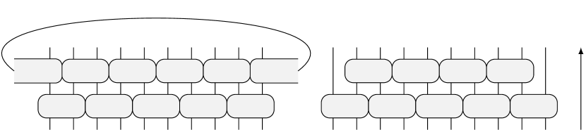
Figure 1: Brickwork circuits acting on $n=10$ qubits. The left and right figures show periodic and open boundary conditions, respectively, and the arrow indicates the direction in which the circuit acts on quantum states. For both of them, the first layer is composed of $n/2$ two-qubit Haar random unitaries acting on qubits $(2i-1,2i),\ i\in[5]$, and the second layer is shifted by one position. On the left, the bricks in the second layer acts on qubits $(2i,2i+1)\,,i\in[5]$, with the periodic identification $n+1=1$. On the right, the second layer acts on qubits $(2i,2i+1)\,,i\in[4]$, leaving the first and the $n$th qubit untouched.

In the following, we derive analytical results for the frame operator of random brickwork circuits with open and periodic boundary conditions. Both BW circuit ensembles are clearly (left and right) invariant under tensor products of single-qubit unitaries, in particular they are right-invariant under Pauli operators. By the preceding discussion in Section 2.2, we thus know that the frame operator $S$ is diagonal in the Pauli basis. It is thus sufficient to compute the matrix elements $(v\,|\kern 0.6458pt\mathopen{}S\kern 0.6458pt|\kern 0.6458pt\mathopen{}v)$ for all $v\in\mathbb{F}_{2}^{2n}$. Moreover, both BW circuit ensembles are also invariant under local Clifford unitaries, i.e. tensor products of single-qubit Clifford gates. This implies that $(v\,|\kern 0.6458pt\mathopen{}S\kern 0.6458pt|\kern 0.6458pt\mathopen{}v)$ is invariant under the exchange of $X$, $Y$, and $Z$ operators, and hence depends only on the weight vector $\operatorname{wt}(v)$. As we show shortly, $(v\,|\kern 0.6458pt\mathopen{}S\kern 0.6458pt|\kern 0.6458pt\mathopen{}v)$ is in fact determined by non-vanishing pairs of elements in $\operatorname{wt}(v)$ corresponding to a brick in the second layer, and by their positions in the circuit. To make this precise, we have to introduce some definitions.

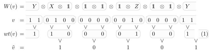
Figure 2: Example how the vector of supported bricks is computed from a 10-qubit Pauli operator. The structure of the shaded bricks is the one of the second layer of the circuit. First, the Pauli operator is transformed into its binary representation $v\in\mathbb{F}_{2}^{20}$. We apply a logical or ($\vee$) per qubit to compute the weight vector $\operatorname{wt}(v)$. Subsequently, this procedure is repeated for qubit pairs $(2i,2i+1)$ and yields the vector of supported bricks $\tilde{v}$. For periodic boundary conditions, the last entry of $\tilde{v}$ is computed between the last and first entry of $\operatorname{wt}(v)$ (here depicted by appending the first entry at the end in parentheses). The brickwork support of this example is $\operatorname{\mathrm{supp}_{\mathrm{BW}}}(v)=\{1,3,5\}$, while its partition into local factors is $\operatorname{\mathrm{part}_{\mathrm{BW}}}(v)=(1,2)$.

Let us consider a Pauli string $v=v_{1}\oplus\dots\oplus v_{n}\in\mathbb{F}_{2}^{2n}$. Roughly speaking, a brick is identified by a pair of two adjacent qubits, and it is in the support of $v$ if at least one of the qubits is in the support of $v$. More formally, we define the vector of supported bricks as

$$\tilde{v}=(\tilde{v}_{1},\dots,\tilde{v}_{n/2})\in\mathbb{F}_{2}^{n/2}\,,\quad\tilde{v}_{i}\coloneqq\operatorname{wt}(v)_{2i}\vee\operatorname{wt}(v)_{2i+1}\,,\quad i\in[n/2]\,,$$ (8)

where $x\vee y$ is the logical or between two bits $x,y\in\mathbb{F}_{2}$, i.e. $x\vee y=1$ if $x=1$ or $y=1$, and $0$ else. The last entry of $\tilde{v}$ is defined according to the boundary conditions of the second layer, in particular $\tilde{v}_{n/2}=\operatorname{wt}(v)_{n}\vee\operatorname{wt}(v)_{1}$ for periodic boundary conditions, and $\tilde{v}_{n/2}\equiv 0$ for open boundary conditions, see also Fig. 2 for an explicit example how $\tilde{v}$ is computed. We say that the $i$th brick in the second layer, with $i\in[n/2]$, is in the support of $v$ if $\tilde{v}_{i}=1$. Then, one can define the brickwork support of $v\in\mathbb{F}_{2}^{2n}$ as $\operatorname{\mathrm{supp}_{\mathrm{BW}}}(v)\coloneqq\{i\mid\tilde{v}_{i}\neq 0\}$. In the following, however, it will be equally important to keep track of sequences of consecutive supported bricks in the circuit. Hence, we introduce the following notation: A one-component of $\tilde{v}$ is a maximal tuple of consecutive ones in $\tilde{v}$, where “consecutive” is again meant w.r.t. the boundary conditions of the BW circuit. Then, we define the partition of the brickwork support $\operatorname{\mathrm{part}_{\mathrm{BW}}}(v)$ to be the integer sequence given by the (non-unique) sizes of the one-components of $\tilde{v}$. For instance, if we have periodic boundary conditions and $\tilde{v}=(1,0,1,0,1)$ as in Fig. 2, then $\operatorname{\mathrm{part}_{\mathrm{BW}}}(v)=(1,2)$. Note that the maximal number of consecutive ones is $n/2-1$ and $n/2$ for open and periodic boundary conditions, respectively.

We can now state our main result:

Theorem 1.

Let $S$ be the frame operator associated with one round of a two-local brickwork circuit with open or periodic boundary conditions in the second layer. Then, $S$ is diagonal in the Pauli basis, and for $v\in\mathbb{F}^{2n}_{2}$

$$(v\,|\kern 0.6458pt\mathopen{}S\kern 0.6458pt|\kern 0.6458pt\mathopen{}v)=\begin{cases}\operatorname{\Sigma_{\mathrm{pb}}}(n)\,,&\quad\operatorname{\mathrm{part}_{\mathrm{BW}}}(v)=(n/2)\,,\\ \prod_{l\in\operatorname{\mathrm{part}_{\mathrm{BW}}}(v)}\operatorname{\Sigma_{\mathrm{ob}}}(2l+2)\,,&\quad\text{otherwise}\,,\end{cases}$$ (9)

where, for any $m\in\mathbb{N}$ even,

$$\operatorname{\Sigma_{\mathrm{pb}}}(m) =\frac{\left(\sqrt{41}+5\right)^{m/2}+(-1)^{m/2}\left(\sqrt{41}-5\right)^{m/2}}{(5\sqrt{2})^{m}}\,,$$ (10)

$$\operatorname{\Sigma_{\mathrm{ob}}}(m) =\frac{5}{2\sqrt{41}}\frac{\left(25-3\sqrt{41}\right)\left(\sqrt{41}+5\right)^{m/2}+(-1)^{m/2+1}\left(25+3\sqrt{41}\right)\left(\sqrt{41}-5\right)^{m/2}}{\left(5\sqrt{2}\right)^{m}}\,.$$ (11)

We provide a proof for the theorem in LABEL:sec:proof_theorem.

Let us briefly comment on the interpretation of the matrix elements of $S$. These values, determined by the elements of $\operatorname{\mathrm{part}_{\mathrm{BW}}}(v)$, are associated with different topologies of the effective BW circuit.

First, notice that the case $\operatorname{\mathrm{part}_{\mathrm{BW}}}(v)=(n/2)$ can occur for periodic boundary conditions only and corresponds to all bricks being in the support of $v$. In particular, for open boundary conditions, the second case in Eq. 9 always applies.

Next, let us motivate the second case in Eq. 9. Concretely, let us first assume $\operatorname{\mathrm{part}_{\mathrm{BW}}}(v)=(n/2-1)$. In the case of open boundary conditions, this assumption corresponds to all bricks being in the support of $v$, since $\tilde{v}_{n/2}=0$ by definition. Likewise, this situation occurs in the BW circuit with periodic boundary conditions whenever there exists exactly one $i\in[n/2]$ such that $\tilde{v}_{i}=0$, see Figure LABEL:fig:brickwork_open_examples. Then, we can make two observations: First, the topology of the effective circuit changes from periodic to open boundary conditions. Second, the effective circuit is equivalent –up to reordering of qubits on which it acts– to the fully supported circuit with open boundary conditions described before, which is depicted in Figure 1.

Suppose now we have a BW circuit with open boundary conditions, and there exists another index $i$ such that $\tilde{v}_{i}=0$. Then, two cases can occur: Either, (a), $i=1$ or $i=n/2-1$, which implies $\operatorname{\mathrm{part}_{\mathrm{BW}}}(v)=(n/2-2)$, and we simply obtain a BW circuit with open boundary conditions on $n-4$ qubits. Otherwise, (b), $\operatorname{\mathrm{part}_{\mathrm{BW}}}(v)=(i-1,n/2-i-1)$ and the BW circuit again factorizes into two independent BW circuits with open boundary conditions, acting on $2i$ and $n-2i$ qubits respectively.

In general, the effective circuit splits into as many independent BW circuits with open boundary conditions as the number of elements in $\operatorname{\mathrm{part}_{\mathrm{BW}}}(v)$, and the diagonal elements of $S$ are given by products of different contributions as in Eq. 9. These elements also determine the number of qubits on which these subcircuits act, see Figure LABEL:fig:brickwork_open_examples for an example with $\lvert$