Radiometric sensitivity and resolution of synthetic tracking imaging for orbital debris monitoring

1OpticalX, Tracy, CA, 95304, USA
2College of Optical Sciences, University of Arizona, Tucson, AZ, 85751, USA

1 Abstract

We consider sampling and detection strategies for solar illuminated space debris. We argue that the lowest detectable debris cross section may be reduced by 10-100x by analysis of phase-space-pixels rather than single frame data. The phase-space-pixel is a weighted stacking of pixels corresponding to a test debris trajectory within the very wide camera field-of-view (FOV). To isolate debris signals from background, exposure time is set to match the time it takes a debris to transit through the instantaneous field of view. Debris signatures are detected though a generalized Hough transform of the data cube. Radiometric analysis of line integrals shows that that sub-cm objects in Low Earth Orbit can be detected and assigned full orbital parameters by this approach.

2 Introduction

Low Earth orbit (LEO), defined as the altitude range between 400-1000 km, contains millions of debris particles that pose significant collision risk to existing spacecraft in operation. For sub-cm objects, the NASA Orbital Debris Program Office conducted studies between the calendar years 2014-2017 using special staring radar modes at the MIT Haystack Observatory in Westford, Massachusetts, and the Goldstone Solar System Radar near Barstow, California Goldstone, each system being able to detect (but not track) 5mm and 3 mm debris, respectively, at altitudes below 1000 km [1]. Per hour, on average 15 (60) debris passed through the extremely narrow beam of 0.058^∘ for Haystack (for 0.037^∘ for Goldstone). The flux for 3 mm debris was measured at 0.03 counts per km². If one to construct a vertical net around the Earth at Goldstone’s latitude of 35^∘ extending between 400-1000 km and wait for 90 mins (typical LEO periods), one would collect approximately 1 million individual sub-cm pieces. Meanwhile, the future looks more cluttery. The number of active satellites has been rapidly increasing as the commercialization of space from LEO to GEO is becoming more attractive for communication and navigation systems. Considering in-flight breakups such as the 2007 Fengyun-1C satellite test, Russia’s test of an anti-satellite weapon in 2021, Iridium 33 and Kosmos 2251 collisions, and a number of accidental satellite fragmenting explosions, debris accumulation will surely accelerate. Ultimately, the concern is that the number of objects in the Low Earth Orbit beyond a certain threshold will trigger the "Kessler effect" [2] that a small number of collisions will trigger an unintended exponentially growing avalanche of fragments, making LEO to GEO unusable. When such an avalanche begins, physically de-orbiting such large number of debris is not feasible. The only option is orbit maneuvering and it requires knowing the orbits of each of the debris pieces as small as mm hours or days ahead of time.

Tracking of sub-cm debris is significantly beyond current capabilities, however. As of September 2022, CelesTrak, a non-profit organization, maintains a catalog of 54000 space objects with sizes approximately 5 cm and larger. Considering that 99.3 percent of debris is below 1 cm [3], the CelesTrak catalog is just the beginning of a lengthy one for true Space Situational Awareness (SSA).

One needs simultaneous scan and stare capability to rapidly look for all the objects in a wide field of view (FOV) while maintaining detection sensitivity. Unfortunately, conventional RF and optical systems trade FOV for sensitivity. Increasing aperture improves sensitivity in staring mode but reduces FOV and detection rate. Moreover, two position measurements are necessary for orbit determination (OD). The likelihood of an object passing through two narrow beams for OD is even smaller. A phased-array, narrow-beam radar, e.g. the Advanced Modular Incoherent Scatter Radar (AMISR) [4] can achieve a wide FOV but the sensitivity at each beam position will decrease by the number of beams. However, this is not true with a 3D computationally post-steering receive array which does increase the sensitivity while maintaining the same FOV On the other hand, the concept of large receive arrays is logistically prohibitive as the number of receivers scales inversely with the 4th power of the debris diameter. Alternatively, one can increase sensitivity using more radar power, however, this requires increasing the already MW+ radar power over multiple orders of magnitude, which is logistically prohibitive or would be a serious environmental concern. A similar argument applies to existing optical systems built for astronomy. Large-aperture deep-space telescopes are extremely sensitive to detect small debris for population statistics but the rate of detections is very small due to the small FOV. Moreover, the angular position and angular rate information from the images is not sufficient for OD which requires linkage of multiple detections that chances of which are small. Finally, Satellite Laser Ranging (SLR) systems are built for precise OD, however, a coarse trajectory is needed for pointing. Just like radars, transmitting high power lidar beams to artificially illuminate debris is problematic.

We discuss here a concept passive optical technique, Space-time Projection Optical Tomography (SPOT), that overcomes the above scan vs. stare problem with the following elements: (1) a massive parallel camera system with a large FOV, (2) massive computational power using Graphical Processing Units (GPUS) that enables synthetic stare capability while rapidly searching a large space of phase-space trajectories in 4-6 dimensions, (3) precise analytical description of debris motion along geodesics allowing astrometric search space optimization, and (4) the Sun to illuminate all millions of debris at the same time with its powerful $\sim$1.36 $kW/m^{2}$ radiation. SPOT can look everywhere within the wide FOV of a survey telescope and can zoom in on each and every particle in the FOV with the sensitivity of a deep-space telescope. The key concept is integrating pixel values corresponding to a track that is precisely defined by orbital parameters. For the limited case of straight tracks, the technique is equivalent to that of 2D Radon transform or to that of 3D Radon transform [5] if a line on a plane is integrated, as in X-ray transform. For 2D transform, two angular parameters and two translational parameters define a line. Here, however, the lines are analytically defined by the orbital two-line element set (TLE), observatory position and observation time. The lines are curved differently; short ones could be analytically described by low order polynomials, while long ones like those of MEO or GEO orbits may require certain spiral forms to describe. In this regard, the transform is best described as a generalized Haugh transform [6]. Interestingly, Haugh was trying to automate the task of detecting and plotting the tracks of sub-atomic particles in bubble chamber photographs[7]. In a collisionless plasma confined by a magnetic field, an energetic electron track can be described by the Lorentz force precisely, just like gravity describes free-fall motion for time intervals short enough to ignore thermospheric drag or other non-gravitational forces. Such analytical precision enables high synthetic exposures by integrating pixels along long track projections on the FOV.

As shown by Shell [8], a single aperture imaging system can detect and track decimeter-scale LEO debris illuminated by the sunlight during twilight hours. Several proof-of-concept single-aperture implementations based on single-pixel thresholding demonstrated detections as small as 10 cm.[9, 10, 11]. Typically, debris detection is done by looking for streaks on single frames. Various algorithms are tasked to identify any streaks on the focal plane that are detectable above the noise. Preceding those algorithms is data preparation to clean known objects such as stars by looking up star catalogs. The tracks are used to calculate angular coordinates and angular velocity and defined as "trackets". Multiple tracklets over multiple sightings are combined to determine an initial orbit as a TLE [12]. For better accuracy, the initial TLE is passed to a more sensitive telescope as cued object or to Satellite Laser Ranging (SLR) stations for precision orbit determination.

A growing literature aims to increase the effective exposure time by integrating pixels over multiple frames under certain assumptions on the trajectories, e.g., moving target indicator,[13] multiple hypothesis testing [14], direct track-before-detect methods [15]. Hough tranform has been used to detect space debris tracks for SSA [16, 17, 18] as well as to clean sky survey databases such as the SuperCOSMOS Sky Survey by detecting and removing such tracks due to various linear phenomena. [19]. Ultimately, the object trajectories are determined by gravity alone over time scales short enough to ignore thermospheric drag. One can form a space of such trajectories depending on the bounds of the orbital regions or on prior orbital information on the object [20] and then apply very selective matched filters to the image database to search for space debris. [21]

Filtering with such extended filter banks and ultimately with exact TLE projections presents an advantage to LEO observations with a wide FOV camera by tightly constraining the orbital parameters. Six parameters are needed to describe a Keplerian orbit. It is generally assumed that the observable states of an optical measurement are angle and angle rates, e.g., ${\bf x}\in\mathbb{R}^{4}$, and no information can be reliably used to determine the other two states representing angular acceleration. [22] This lead to the definition of admissible regions or a region of hypotheses consistent with a particular $\mathbb{R}^{4}$ observation. [20] While the $\mathbb{R}^{4}$ assumption is largely true for GEO due to the large radial distance to the object and very low angular rates that do not change over the relatively narrow FOV, LEO is very different. LEO has very high angular rates which change significantly from near zenith to near horizon. Such angular rate variations can be captured by a wide FOV camera design providing the other two undetermined states. Thus optical measurements that enable ${\bf x}\in\mathbb{R}^{6}$ including angular acceleration significantly constrains the search space enabling the discovery of LEO objects with full orbital parameters.

SPOT is designed to search the $\mathbb{R}^{6}$ space for uncued discovery of sub-cm and larger geocentric objects by simultaneously achieving high sensitivity and high search rates using computationally intensive synthetic tracking algorithms. The algorithm is analogous to computationally zooming in on runway sequential flashing lights also known as "rabbit lights" in aviation. Since the debris is so faint, the idea is to use very short exposure time per frame (to minimize background) while maximizing the signal exposure time by stacking only the pixels that contain the signal. This methodology is similar to the algorithms successfully used to detect faint objects in the asteroid belt. [23, 24, 25, 26, 27] except the time scales for Earth-orbiting objects are much faster. For LEO, SPOT can stare at each debris for up to 10 mins although the transit time through each pixel is as short as 10 ms. This synthetic maximization of the exposure time is key to detect sub-cm debris, while the ability to search in the wide FOV is key to cataloging large number of debris per unit time.

Below, we review Shell’s radiometric analysis for single-pixel SNR and then extend the calculations to multi-pixel integrals over the entire FOV to maximize the incorporation of all information from the measured images. We compute cumulative SNR for sample LEO and MEO trajectories and for various debris sizes. We then briefly discuss phase-space-pixel resolution and how it related to orbital parameters.

3 Single-pixel SNR dependency on exposure time

The photoelectron content of a pixel is due to (1) $e_{s}=e_{s0}\tau_{t}$: signal photons acquired during the object transit time $\tau_{t}$ through the pixel, (2) $e_{b}=e_{b0}\tau_{e}$: background photons acquired during the exposure time $\tau_{e}$, (3)$e_{n}$: the detector noise per reading and (4) unwanted photons coming from other distinct objects like stars and man-made objects. For simplicity, lets ignore (4) and assume best efforts are made to mask the associated pixels. Here, the radiometric values $e_{s0}$ and $e_{b0}$ are detailed in the next section. Then,

$$e_{total}=e_{s0}\tau_{t}+e_{b0}\tau_{e}+e_{n}$$ (1)

For a particular observing geometry $\tau_{t}$ is already determined for each pixel. Now, we look for the best $\tau_{e}$ to maximize the single-pixel SNR. For $\tau_{e}>\tau_{t}$, it is given by

$$SNR_{\tau_{e}\geq\tau_{t}}=\frac{e_{s0}\tau_{t}}{\sqrt{e_{b0}\tau_{e}+e_{n}^{2}}}$$ (2)

and it maximizes when $\tau_{e}=\tau_{t}$. This is easy to see because, beyond the object transit time, the pixel is no longer collecting signal photons while continuing to accumulate background photons. However, for $\tau_{e}<\tau_{t}$,

$$SNR_{\tau_{e}\leq\tau_{t}}=\frac{e_{s0}\tau_{e}}{\sqrt{e_{b0}\tau_{e}+e_{n}^{2}}}$$ (3)

Here again the SNR maximizes when $\tau_{e}=\tau_{t}$ because it is an increasing function of $\tau_{e}$. Therefore, the best SNR for a pixel box is achieved when the exposure time is equal to the transit time. We discuss below how the transit time depends on the sensor size and how too-small of a transit time is a problem in the presence of read noise. Generally, the telescope and camera parameters are chosen with the read noise setting a lower bound on the tolerable background noise. As can be seen from Eq. 2, if the background noise is already much smaller than the read noise, shortening the exposure time further does not significantly enhance the SNR and the resulting higher frame unnecessarily adds to the data acquisition and processing burden.

The line that pierces through pixels of a data cube, i.e., stacks of frames with each frame $\tau_{e}$ thick, is the projection of an Earth-centered Keplerian orbit. Each pixel box of the data cube on the line will capture various fractions of the signal photoelectrons. Now, the problem of finding debris may be formalized as follows: determine if a line of pixels corresponding to a particular orbit occupied. As we discussed above, that line of pixels is represented by a phase-space-pixel (PSP), a point in a six-dimensional space. It is a generalization of the ’vector-pixel’ as used in [26] for constant angular speed objects.

4 Radiometric equation for a phase-space-pixel

The number of signal ($e_{s}$) and background ($e_{b}$) photoelectrons from a single detector pixel are respectively given by [8]

$$e_{s} = QE\cdot\tau\cdot A\cdot\tau_{atm}\cdot E_{RSO}\cdot\tau_{t}~{}~{}~{}~{}~{}~{}~{}[e^{-}]$$ (4)

$$e_{b} = QE\cdot\tau\cdot A\cdot L_{B}\cdot\frac{x^{2}}{f^{2}}\cdot t_{e}~{}~{}~{}~{}~{}~{}~{}[e^{-}]$$ (5)

wherein $QE$ is quantum efficient, $\tau$ is optical transmittance, $A$ is aperture area, $\tau_{atm}$ is atmospheric transmittance, $x$ is pixel size, and $f$ is focal length.

The Resident Space Object (RSO) visual magnitude $E_{RSO}$ is given by [8]

$$E_{RSO}=5.6\times 10^{1}0\cdot 10^{-0.4m_{sun}}\cdot\frac{d^{2}}{R^{2}}[0.25\rho_{\rm spec}+\rho_{\rm diff}p_{\rm diff}(\psi)]$$ (6)

where $m_{sun}$ is the visual magnitude of the Sun (-26.7), $d$ is the RSO diameter and $R$ is the range, $\rho_{\rm spec}$ and $\rho_{\rm diff}$ are specular and diffuse components of the RSO albedo ($\rho=$0.175 is equally split), the latter being a function of the solar phase angle $\psi$ as follows:

$$p_{\rm diff}(\psi)=\frac{2}{3\pi}[\sin(\psi)+(\pi-\psi)\cdot\cos(\psi)]$$ (7)

The atmospheric background $L_{B0}$ at zenith (photons per second per meter squared per steradian) is given by

$$L_{B0}[i,j,k]=5.6\times 10^{1}0\cdot 10^{-0.4m_{b}}\cdot(\frac{180}{\pi})^{2}\cdot 3600^{2}$$ (8)

and $m_{b}$ is background in units of visual magnitudes per square arc seconds. That is, it is a measure of visual magnitude spread out over a square arcsecond of the sky. For a given $m_{b}$, smaller IFOV will result in smaller background noise per pixel. A truly dark sky has $m_{b}=$21.8 mag arcsec^-2. The sky at its zenith gets darker by $\approx 0.4$ mag arcsec^-2 during the first six hours after the end of twilight (sun 6 deg below). [28]. The time variation will be ignored here, however. Instead, we will use zenith angle dependence. To calculate the background at $z$ degrees off zenith we use

$$L_{B}=L_{B0}[0.4+0.6\cdot(1-0.96\sin^{2}z)^{-1/2}]$$ (9)

This formula by Garstand [29] is based on the analysis by Roach and Meinel [1955] [30], in which 40 percent of the average faint star background) and 60 percent comes airglow emissions at a height 130 km. We compared this $z$ dependence against the analytical form by Shell [8] and found agreement within a magnitude of less than 1.

For detector noise, we will assume no dark current and use an RMS value of 1 for read noise $e_{n}$. Then, the SNR for a single pixel is given by

$$SNR=\frac{e_{s}}{\sqrt{e_{b}+e_{n}^{2}}}$$ (10)

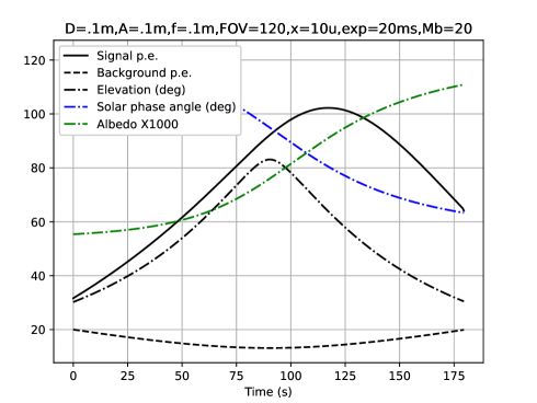
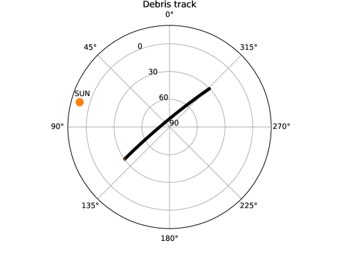
Figure 1: (Left) Variation of single-pixel signal and background photoelectrons, debris elevation, solar phase angle, and debris albedo along the path shown on the right. Here, $d=10$ cm, $A=10$ cm, $f=10$ cm, and $x=10~{}\mu$. The exposure time for $e_{b}$ is $20$ ms. To calculate $e_{s}$, we use the pixel transit time $t_{t}$ which varies along the trajectory. (Right) The test debris track from an ISS TLE used for the single=pixel analysis on the left and the PSP SNR analysis below. The track is moving in the NW direction (away from the Sun shown by the orange dot).

Figure 1 (right) shows a sample debris track corresponding to the following TLE, which belongs to the International Space Station (ISS):

1 25544U 98067A 22241.38033696 .00006975 00000+0 13024 3 0  9998
2 25544 51.6450 333.9762 0003281 173.1914 302.2976 15.49962082356533

The elevation and azimuth track is as seen from a location near San Francisco, CA, looking up. The $3$ min pass above $30^{\circ}$ elevation is during morning twilight; the Sun is at $\approx 11^{\circ}$ below the horizon. This pass is chosen because of its high peak elevation providing a simple geometry to analyze the effect of some of the radiometric parameters. Figure 1 (right) shows the variation of the single-pixel signal and background electrons along the track for 10 cm debris. The exposure time $\tau_{e}$ is chosen as 20 ms for calculating the background noise while $\tau_{t}$ (for signal photons) is variable and given by the debris transit time through apixel. Note that the background is symmetric around the peak elevation (near 90 s) and increases with decreasing elevation as a result of Eq. 9. Moreover, the skewness of the $e_{s}$ curve is due to the albedo dependence on the solar phase angle (Eq. 7).

Figure 1 (left) shows the variation of the single-pixel signal and background electrons along the track for 10 cm debris. The exposure time $\tau_{e}$ is chosen as 20 ms for calculating the background noise while $\tau_{t}$ (for signal photons) is variable and given by the debris transit time through a pixel (dotted line). Note that the background is symmetric around the peak elevation (near 90 s) and significantly decreases with decreasing elevation as a result of equation X. Thus, at low elevations and short exposure times read noise contribution becomes dominant. Moreover, the skewness of the $e_{s}$ curve is due to the solar phase function given in Equation X.

To obtain the radiometric equation for a PSP, we choose a hypothetical track $T[\theta_{x}(t),\phi_{x}(t)]$ as the angular trace of a moving hypothetical object as viewed from a position $\bf x$. Next, we define a 3D pixel as $[i(t),j(t),k(t)]$ wherein $(i,j)$ are spatial indices and $k$ is the image frame number, all step functions of $t$. We assume no space or time gaps between pixels such that for each time $t$ the object angular position can be associated with a unique pixel. The task is to computationally zoom in on the moving object by integrating over the pixels containing the object.

For simplicity, we assume the camera is mechanically fixed, although it does not have to be. We also assume that the camera orientation, pointing and lens distortion is calibrated to a small fraction of a pixel such that the effect of pointing uncertainties are negligible. Such calibration can be achieved by matching the location of a large database of bright points sources such as the ESA’s Hipparcos space astrometry database which provides the positions of more than one hundred thousand stars with high precision. Another source is the JPL ephemeris DE421 for the planets.

Note a debris track $T$ can be accurately described by models including gravity and non-gravitational forces over the FOV such that its position perturbation due to unknown drag forces is much smaller than the physical dimensions of a 3D pixel. For example, the maximum deceleration due to the atmospheric drag of a 10 cm cube object with a density of 1$\rm g/cm^{3}$ (Area-to-Mass-ratio (AMR) is 0.01) at 780 km altitude is $10^{-9.5}{\rm km/s}^{2}$ [31]. The position perturbation from the beginning to the end of a 1000 s long track will be 15 cm. This perturbations for a cm cube and a mm cube will be 1.5 m and 15 m, respectively, still small numbers compared to the 25-100 m IFOV of telescope at 780 km. The drag perturbations are modeled into orbit predictions, thus, the effect of unknown forces is minuscule and the effect on the accuracy of FOV projections is negligible.

Continuing with the radiometric analysis, instead of SNR thresholding of a single-pixel for detection as is done in Shell[8], we SNR threshold the phase-space pixel, a weighted integral of the pixel values corresponding to a track. Then, the line integral of the signal photoelectrons $e_{s}^{L}$ can be expressed as:

$$e_{s}^{L}=QE\cdot A\cdot\tau\int_{a}^{b}\tau_{atm}(t)E_{RSO}(t)dt$$ (11)

where $\tau_{atm}(t)$ and $E_{RSO}(t)$ are now time-dependent because the range $R$, solar phase angle $\Phi$, and the atmospheric penetration angle is changing as the debris moves. Note that no "pixellation" exists in the above integral; the assumption is that the selection of the pixel boxes $(i,j,k)$ will contain 100$\%$ of the signal photoelectrons.

The line integral of the background noise is given by

$$e_{b}^{L}=QE\cdot A\cdot\tau\cdot\frac{x^{2}}{f^{2}}\sum_{(i,j,k)\in T}L_{B}[i,j,k]\tau_{e}[i,j,k]$$ (12)

where $\tau_{e}[i,j,k]$ is the exposure time of the pixel $[i,j,k]$. While pixel-dependent exposure time is not expected from a single camera, for multiple cameras covering low and high elevation, a variable exposure time may be used. Note that, in contrast to $e_{s}^{L}$ which is a continuous integral, $e_{b}^{L}$ is a discrete integral. The main reason for this is $\tau_{t}$ is a continuously changing variable while $\tau_{e}$ is preset as a system parameter.

Similar, the line integral of the read noise is a discrete sum,

$$e_{n}^{L}=\sqrt{\sum_{(i,j,k)\in T}e_{n}[i,j,k]}$$ (13)

where we made $e_{n}$ a function of pixel location in case multiple cameras with different read noise characteristics are used.

Then, the line integral SNR is given by

$$SNR^{L}=\frac{e_{s}^{L}}{\sqrt{e_{b}^{L}+(e_{n}^{L})^{2}}}$$ (14)

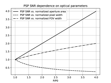
Figure 2: PSP SNR dependence on the normalized system parameters: aperture area, pixel size and FOV extent. The focal length is set equal to the aperture diameter. When changing the aperture area, FOV is kept constant by changing the number of telescopes. Read noise is ignored.

Figure 2 shows how PSP SNR changes as a function of normalized system parameters. If the read noise is negligible compared to the background noise, we arrive at the following analysis. Assume that the system captures a fixed duration of a debris track, which means fixed FOV. If the aperture diameter and focal length increases by 2, $SNR^{L}$ increases by 4. Note $e_{s}^{L}$ increases by 4 but $e_{b}^{L}$ remains the same. This is so because although the number of pixels along the track increase by two because of the halving of IFOV, the exposure time $\tau_{e}$ will be halved to match the halved transit time through a pixel. Then, since $e_{b}^{L}$ is proportional to $A$ and IFOV², it will remain the same.

If the read noise is the dominant source of noise, we arrive at a different analysis. If the aperture diameter and focal length increases by 2, $SNR^{L}$ increases by $2\sqrt{2}$. Note $e_{s}^{L}$ increases by 4 but $(e_{n}^{L})^{2}$ increases by 2, because twice the number of pixels are read.

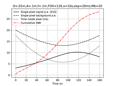
Figure 3: Cumulative $SNR^{L}$ (red dashed line) for the debris pass shown in Figure 1 but for a 1 cm debris. Also shown are single-pixel SNR (solid black line), background (dashed black line) and time spent inside a pixel (dotted line). The optical parameters are: $d_{\rm deb}=$1 cm, $d_{\rm aperture}=$10 cm,$f=$10 cm, $x=$10 $\mu$, $\tau_{E}=20$ ms.

Figure 3 shows the single-pixel signal and background photoelectrons for a 1 cm debris as well as the cumulative (0-t) $SNR^{L}$ (red line) for the track shown on the RHS of 1. We used $m_{b}=$20.0 mag arcsec^-2, a conservative value considering the observed range of 20-22 mag arcsec^-2 (European Southern Observatory - Paranal) [32]. $SNR^{L}$ reaches an easily detectable level of 14 by the end of the track. The track passed through 20768 pixels and accumulated a total of 180 s of effective signal photon exposure while the accumulated background photon exposure was 415 s (the single-pixel background photon exposure was fixed at $\tau_{E}=$20 ms). Similarly, the read noise is proportional to the number of pixels read and given by $e_{n}^{2}={\rm 20768}\times e_{n0}^{2}$. Here, we used $e_{n0}=1$ RMS.

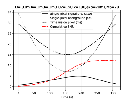
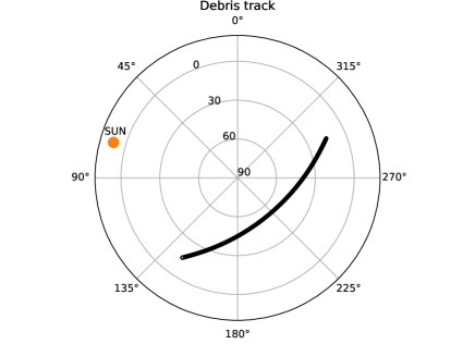
Figure 4: The same pass as Figure 3 but viewed from a 4^∘ higher location in latitude.

Figure 4 (right) shows the same debris pass but viewed from a location 4^∘ higher in latitude. This time the section of the track with $15^{\circ}+$ elevation is shown. The duration is 620 s and the debris was sunlit during the entire track shown. Despite being $\sim$3.5 times longer, the $SNR^{L}$ reaches only $\sim$7 about half of the $SNR^{L}$ for the overhead pass shown in Figure 3. Inspecting both figures, $R^{2}$ drop in number of signal photons and higher background at lower elevations are responsible for the lower $SNR^{L}$ of the low-elevation pass. Also, it can be seen that $SNR^{L}$ rises fastest near the time of the peak elevation.

Note in performing the integrations, it is assumed that the track is going through the center of pixels such that cross-track neighbors have no contribution. In reality, this is not the case due to the finite width of the point spread function (PSF) and possibly double or triple the number of pixels are involved. In that case, the effective integrated signal photon exposure will remain the same but the integrated background will increase proportionally to the number of pixels involved, resulting in a reduced $SNR^{L}$ by a factor of 1.5-2.

Finally, for completeness, the $SNR^{L,M}$ of a cluster of $M$ identical cameras placed adjacently and looking in the same direction is given by

$$SNR^{L,M}=\frac{Me_{s}^{L}}{\sqrt{Me_{b}^{L}+M(e_{n}^{L})^{2}}}=\sqrt{M}SNR^{L}$$ (15)

If one is to pursue increasing radiometric sensitivity to extreme limits by deploying such clusters in massive numbers, the detectable debris diameter will decrease with the 4th power of the number of cameras in the cluster,

$$D_{detectable}\propto M^{1/4}$$

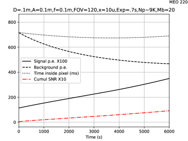
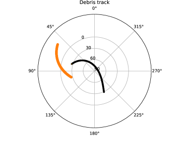
Figure 5: MEO orbit (22000 km). Cumulative $SNR^{L}$ (red dashed line) for a 10 cm debris in MEO (22000 km). The trajectory corresponds to a GPS satellite TLE (Navstar 56). The orange line is the Sun’s trajectory. Also shown are single-pixel SNR (solid black line), background (dashed black line) and time spent inside a pixel (dotted line). The optical parameters are: $d_{aperture}=$10 cm,$f=$10 cm, $x=$10 $\mu$,$\tau_{E}=$700 ms.

Thus far, we considered LEO. Higher orbits are slower in angular rate, thus exposure times per pixel will be longer. Figure 5 shows the cumulative SNR of a 10 cm m debris in Middle Earth Orbit (MEO) with the same telescopic parameters used so far. The simulated orbit is that of the GPS satellite navstar 56. Note the exposure time (500-700 ms) is significantly longer than that of LEO (10 ms). While single-pixel SNR is between $\sim 0.05-0.2$ (not shown on the plot), $SNR^{L}$ reaches $\sim 8$ after integrating about $\sim$9000 pixels over $\sim$1.6 hours. While such hour-like long line integrals sound daunting computationally, they are simply slow-motion versions of the LEO integrals, with the number of pixels per integration remaining the same. The projection line forms are significantly different, however, and how it effects the computations will be investigated in a separate study.

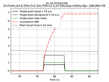
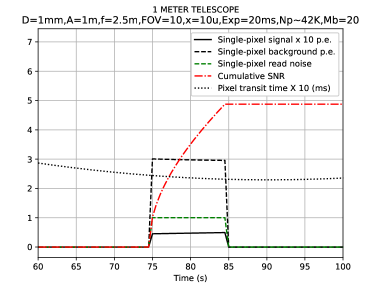
Figure 6: Cumulative SNR for an array of 25-cm (left) and an array of 1-m telescopes (right) for the orbit shown in Figure 1. The number of telescope are chosen to provide FOVs of 2.3^∘ and 10^∘, respectively. A constant exposure time of 20 ms is used for both systems.

We have shown thus far that it is theoretically possible to detect and track realistic size operational spacecraft ($>10{\rm cm}$) from LEO to GEO and objects as small as 1 cm in LEO with a modest 10 cm aperture telescope computing phase-space-pixels. Ultimately, we are interested in an SSA solution with a sensitivity to detect and track sub-cm debris and that solution will require more aperture.

Figure 6 shows the SNR performance for an array of 0.25m (left) and 1 m (right) aperture telescopes providing significantly greater sensitivity to detect 5 mm and 1 mm debris, respectively. The same orbit in Figure 1 is used except the FOV is 2.3^∘ for the 25 CM system and 10^∘ for the 1-m system. Note that both systems have the same iFOV, i.e., $x/f$. Although the exposure times are fixed at 20 ms, the single-pixel background photoelectrons are different because of the $\times 16$ aperture area difference. For the 25-CM system, the background is about 0.3, a small fraction of the read noise, whereas for the 1-m system, it is 3X read noise.

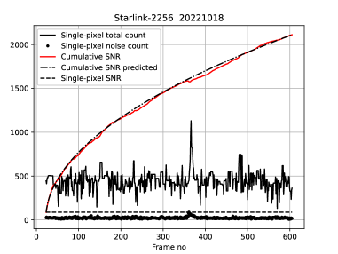
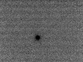
Figure 7: Starlink-2256 captured by a single William Optics telescope at 200 FPS. (Left) The cumulative SNR (red curve) matches well the predicted SNR (based on the $\sqrt{N}$ rule). Shown also is the single-pixel SNR obtained from averaged single-pixel signal and noise values. (Right) Average of $\approx$600 frames corresponding to an effective exposure of 3 s. The faint diagonal line is the satellite passing by Sirius, the brightest star in the night sky.

Figure 7 shows data for the Starlink-2256 pass captured by a single William Optics telescope (1.2^∘ FOV ) on 10/18/2022. The images were captured at 200 fps and the object was located ahead of time using Stellarium. A single-pixel-detection based tracking algorithm was developed to find the $(i,j)$ path. The signal was integrated along this path. The cumulative SNR grows proportional to $\sqrt{N}$ as predicted. The image on the right is an average of all the frames throughout the 3 s pass and the Starlink track is distinguishable as the diagonal line.

5 Phase-space-pixel resolution and the search space

We defined phase-space-pixel or PSP as the sum of the values of all the pixels that line up on the projection of a hypothetical phase-space trajectory on the camera FOV. The terminology phase space can be used for any multidimensional space, however; it does not have to be a space of position and velocity only. Just as $[i,j]$ uniquely identify a pixel, here we see an orbit as a one unique point in a six-dimensional phase space. If we can properly define the resolution of that one point, we can calculate orbital uncertainty and the number of grains we have to sort through to find the object.

PSP resolution can be understood as follows. In two-dimensions, the angular resolution of a conventional pixel camera can be defined by the angular extent by which two closely-spaced point sources in $\mathbb{R2}$ can be distinguished. It corresponds to a grain of steradian at an azimuth and elevation point. In four-dimensions, the resolution of a vector-pixel, as used by [26], can be defined as the extent two closely-spaced constant-angular speed point sources in angular phase-space can be distinguished. This is how MEO-GEO or Near-Earth-Orbit (EO) observations are modeled. The object has two angular position and 2 angular speed variables and one performs a search in the $\mathbb{R2}$ space by computing vector-pixels as sum of pixels corresponding to an angular phase-space trajectory. For long integration times over a wide FOV, vector-pixel does not have enough dimensions to describe the track as the angular speed changes within the FOV. We therefore compute PSP over a six dimensional phase-space trajectory parametrized by the orbital elements. Then, the PSP resolution can be defined as the extent two closely-spaced accelerating point sources in R6 can be distinguished.

Phase-space-resolution can be computed as follows. A point source with a hypothetical orbit excites photoelectrons on a line of pixels which can be termed as "line spread function" or LSF such that the cross-track width is given by the point-spread function (PSF). For simplicity, we will assume PSF is a delta function, therefore, LSF is an infinitely thin stripe. This means only one pixel, the one whose boundaries contain the debris, is activated at a time. PSP resolution can therefore be defined as the 6D grain size at a given position in the R6 space. The grain size can also interpreted as the orbital uncertainty defined as the coarseness of orbital parameters that are consistent with the given measurements [33].

The boundaries of the grain can be defined such that throughout the volume of a grain, half of the projection pixels remain the same. To determine the 6D grain size for an orbit ${\bf x}=[\theta,\Omega,e,\omega,M,r]^{T}$ that starts at time $t_{0}$ and ends at $t_{1}$, we first compute the corresponding pixel positions

$$(i,j,k)\in L_{t_{0}}^{t_{1}}({\bf x})$$ (16)

where $[i,j]$ are the row and column positions of the $k$th frame and $L$ is the LSF. The $R^{6}$ parameters above are inclination ($\theta$), longitude of the ascending node ($\Omega$), eccentricity ($e$), argument of perigee ($\omega$), mean anomaly ($M$) and revolutions per day ($r$). If the time interval $t_{0}-t_{1}$ is such that the orbital segment is outside the FOV, $(i,j,k)$ will be an empty set ($\varnothing$). Generally, we can choose $t_{0},t_{1}$ to correspond to entry and exit times at the FOV perimeter pixels. Moreover, to maximize the exposure time $\delta_{\tau}=t_{1}-t_{0}$, we can avoid computing trajectories that marginally pass through the FOV, like those clipping the corner of the imaged area. For the following analysis, we will assume a trajectory that is fully contained in the FOV. To compute the resolution in $\theta$, we first compute the set

$$A=(i,j,k)\in L(\theta,\Omega,e,\omega,M,r)$$

Then, we compute the set for the same trajectory but increment by $\Delta\theta$ in inclination:

$$B=(i,j,k)\in L(\theta+\Delta\theta,\Omega,e,\omega,M,r)$$

The resolution in inclination is given by the increment that results in exactly half the pixels common to both trajectories, i.e.,

$$\theta_{resolution}=arg_{\Delta\theta}n(A\cap B)=n(A)/2.$$

We do the same procedure to compute the resolution for the other dimensions.

Here we compute resolutions for a test orbit for the camera system discussed above. We use an NxN pixel camera pointed at zenith and locate the observatory at the equator at 0$\circ$ longitude. We will use a test orbit that overflies the observatory at $h=$420 km with speed 7672 m/s and passes through its zenith at $t=0$. The test orbit has the following parameters: $\theta=90,\Omega=360.0,e=0,\omega=0,M=0,r=15.49962$, which correspond to a 90^∘ inclination circular orbit at an altitude of 420 km. Due to the Earth’s rotation, the test object approaches zenith from 176^∘ azimuth and departs 356^∘ azimuth.

We now change each of the 6 orbit parameters in small increments until we find the increment that correspond to a set $B=(i,j,k)$ such that only 50 percent of the pixels are common with the original set $A=(i,j,k)$ We do this for $N=10,100,1000,10000$. Table 1 shows the grain sizes for all the orbital parameters with the exception of $e$ and $\omega$ since we assumed the test orbit is circular. We can arrived at the following analysis. If the track can be approximated as a straight line on the image, orbit inclination ($\theta$) corresponds to track slope and longer tracks (higher $N$) give higher resolution. Since the slope on an $NxN$ frame can be determined roughly with a precision of $1$ pixel over $N$ pixels, the numbers for $d\theta$ for different $N$ are roughly given by $\arctan(1/N)$. Next, an increment of $\Omega$ corresponds to shift of the track to the left or right and, again assuming a straight track, the resolution d$\Omega$ is independent of the track length and it roughly corresponds to a $\Omega$ shift that corresponds to lateral movement of the track by half a pixel. Therefore, cross-track spatial resolution can be determined to a resolution of $(x/2f)\times$ h = 21 m. Next, $r$ resolution is inversely proportional to $N$. This is so because the angular rate, which is proportional to $r$, can be determined to a precision of $\tau_{e}/N$, where $\tau_{e}$ is the exposure time or the inverse of the frame rate. The $dr$ values in Table 1 correspond to 23, 8.7, 0.87, and 0.087 km, respectively. Finally, the mean anomaly resolution is determined by $\tau_{e}$. Here we used an exposure time of $5$ ms. Considering the 92.9 min orbit here, we get $360.0^{\circ}\times 5ms/(92.9min\times 60s)=0.000161^{\circ}$, which closely matches $dM$ in Table 1. This means the along-track position can be determined to a resolution of 7672 m/s $\times$ 5 ms = 38 m.

N (pixels)	10	100	1000	10000
$d\theta$ (deg)	3.04	1.21	0.13	0.013
$d\Omega$ (deg)	0.000180	0.000176	0.000175	0.000174
$dr$ (rev/day)	0.079	0.030	0.003	0.0003
$dM$ (deg)	0.000175	0.000175	0.000175	0.000187

Table 1: Computationally-obtained track resolutions for a northbound LEO test circular orbit in LEO overflying through the zenith of an optical observatory located at the equator for a range of $NXN$ camera systems with the same IFOV. $dr$ can be converted to altitude resolution $dh$ by multiplying it by $\approx 300$, e.g., $dh\approx 0.1$ km for $N=10000$.

6 Conclusion

The performance calculations using a geodesic line integral formulation show that sub-cm debris can be detected and tracked by a generalized Hough transform of data from arrays of cameras positioned to provide a wide FOV to maximize the light collected off debris during twilight hours. Compared to a single-pixel signal-to-noise ratio, the line integral SNR dramatically increases roughly proportional to the square root of the number of pixels along the track, implying the significance of synthetically-built exposure time. We show that such line integrals not only increase the sensitivity but also provide meter-scale resolution in locating the object. Such increase in sensitivity and resolution comes with a heavy computational cost which requires computing trillions or more tracks per second. The computational task and orbit determination will be discussed in a companion paper.

References

- [1] T. Kennedy, J. Murray, and R. Miller, “Recent radar observations of the sub-centimeter orbital debris environment,” \JournalTitleIAA Conference on Space Situational Awareness (2020).
- [2] D. J. Kessler and B. G. Cour-Palais, “Collision frequency of artificial satellites: The creation of a debris belt,” \JournalTitleJournal of Geophysical Research 83, A6 (1978).
- [3] C. G. Lee, M. A. Slade, J. S. Jao, and N. Rodriguez-Alvarez, “Micro-meteoroid and orbital debris radar from goldstone radar observations,” \JournalTitleJournal of Space Safety Engineering 7,3, 242–248 (2020).
- [4] T. Valentic, J. Buonocore, M. Cousins, C. Heinselman, J. Jorgensen, J. Kelly, and A. V. Eyken, “Amisr the advanced modular incoherent scatter radar,” \JournalTitleIEEE International Symposium on Phased Array Systems and Technology pp. 659–663 (2013).
- [5] P. A. Toft, “The radon transform - theory and implementation,” Ph.D. thesis, Technical University of Denmark (1996).
- [6] P. V. C. Hough, “A method and means for recognising complex patterns,” \JournalTitleU.S. Patent 3,069,654 (1962).
- [7] P. E. Hart, “How the hough transform was invented,” \JournalTitleIEEE Signal Processing Magazine pp. 18–22 (2009).
- [8] J. R. Shell, “Optimizing orbital debris monitoring with optical telescopes,” \JournalTitle2010 Advanced Maui Optical and Space Surveillance Technologies Conference, 14-17 Sep, Maui, HI. (2010).
- [9] P. Wagner and T. Clausen, “Apparillo: a fully operational and autonomous staring system for leo debris detection,” \JournalTitleCEAS Space J pp. 303–326 (2022).
- [10] P. Wagner, D. Hampf, and W. Riede, “Passive optical space surveillance system for initial leo object detection,” \JournalTitleProceedings of 66th International Astronautical Conference (2015).
- [11] T. Hasenohr, D. Hampf, and P. Wagner, “Initial detection of low earth orbit objects through passive optical wide angle imaging systems,” \JournalTitleProc. of Deutscher Luft- und Raumfahrtkongress (2016).
- [12] A. Lue, J. D. Ruprecht, J. Varey, M. Czerwinski, and H. E. Viggh, “Discovering the smallest observed near-earth objects with the space surveillance telescope,” \JournalTitleIcarus 325 (2019).
- [13] D. F. Kostishack, B. E. Burke, and G. J. Mayer, “Continuous-scan charge-coupled device (ccd) sensor system with moving target indicator (mti) for satellite surveillance,” \JournalTitleSPIE Smart Sensors II. (1980).
- [14] J. C. Zingarelli, E. Pearce, R. Lambour, T. Blake, C. J. Peterson, and S. Cain, “Improving the space surveillance telescope’s performance using multi-hypothesis testing. the astronomical journal,” \JournalTitleThe Astronomical Journal p. 111 (2014).
- [15] S. J. Davey, M. G. Rutten, and N. J. Gordon, “Track-before-detect techniques,” \JournalTitleIntegrated Tracking, Classification, and Sensor Management pp. 311–362 (2013).
- [16] M. Svedlow and P. Semenza, “Application of the hough transform to track detection,” \JournalTitle31st Aerospace Sciences Meeting (1993).
- [17] G. Privett, S. George, W. Feline, A. Ash, and G. Routledge, “An autonomous data reduction pipeline for wide angle eo systems,” \JournalTitle2017 Advanced Maui Optical and Space Surveillance Technologies Conference (2017).
- [18] P. Jiang, C. Liu, W. Yang, and Z. Kang, “Automatic space debris extraction channel based on large field of view photoelectric detection system,” \JournalTitlePublications of the Astronomical Society of the Pacific p. 024503 (2022).
- [19] A. J. Storkey, N. C. Hambly, C. K. I. Williams, and R. G. Mann, “Cleaning sky survey data bases using hough transform and renewal string approaches,” \JournalTitleMonthly Notices of the Royal Astronomical Society pp. 36–51 (2004).
- [20] T. S. Murphy, “Integrated tasking, processing, and orbit determination for optical sensors in a space situational awareness framework,” Ph.D. thesis, Georgia Institute of Technology (2018).
- [21] T. S. Murphy, M. J. Holzinger, and B. Flewelling, “Space object detection in images using matched filter bank and bayesian update,” \JournalTitleJGCD (2016).
- [22] A. Milani, G. F. Gronchi, M. D. Vitturi, and Z. Knezevic, “Orbit determination with very short arcs. i admissible regions,” \JournalTitleCelestial Mechanics and Dynamical Astronomy 90, 1-2 (2004).
- [23] M. Shao, B. Nemati, C. Zhai, S. G. Turyshev, J. Sandhu, G. Hallinan, and L. K. Harding, “Finding very small near-earth asteroids using synthetic tracking,” \JournalTitleThe Astrophysical Journal 782:1 (2014).
- [24] C. Zhai, M. Shao, B. Nemati, T. Werne, H. Zhou, S. G. Turyshev, J. Sandhu, G. Hallinan, and L. K. Harding, “Detection of a faint fast-moving near-earth asteroid using the synthetic tracking technique,” \JournalTitleThe Astrophysical Journal 792:60 (2014).
- [25] C. Zhai, Q. Ye, M. Shao, R. Trahan, N. S. Saini, J. Shen, T. A. Prince, E. C. Bell, M. J. Graham, G. Helou, S. R. Kulkarni, T. Kupfer, R. R. Laher, A. Mahabal, F. J. Masci, B. Rusholme, P. Rosnet, and D. L. Shupe, “Synthetic tracking using ztf deep drilling data sets,” \JournalTitlePublications of the Astronomical Society of the Pacific 132:064502 (2020).
- [26] A. N. Heinze, S. Metchev, and J. Trollo, “Digital tracking observations can discover asteroids 10 times fainter than conventional searches,” \JournalTitleThe Astrophysical Journal 150:125 (2015).
- [27] A. N. Heinze, J. Trollo, and S. Metchev, “The flux distribution and sky density of 25th magnitude main belt asteroids,” \JournalTitleThe Astrophysical Journal 158:232 (2019).
- [28] M. F. Walker, “The effect of solar activity on the v and b band sky brightness.” \JournalTitlePublications of the Astronomical Society of the Pacific p. 496 (1988).
- [29] R. H. Garstang, “Night-sky brightness at observatories and sites,” \JournalTitlePublications of the Astronomical Society of the Pacific pp. 306–329 (1989).
- [30] F. E. Roach and A. B. Meinel, “Nightglow heights : a reinterpretation of old data,” \JournalTitleAstrophysical Journal p. 554 (1955).
- [31] E. Montenbruck and G. Eberhard, “Satellite orbits,” in Satellite orbits, (2000).
- [32] F. Patat, “Ubvri night sky brightness during sunspot maximum at eso-paranal,” \JournalTitleAstronomy and Astrophysics 400, 1183–1198 (2003).
- [33] Z. Folcik, A. Lue, and J. Vatsky, “Reconciling covariances with reliable orbital uncertainty,” \JournalTitleAMOS Technology Conference and Exhibit. Maui, Hawaii (2011).