Extending Logic Explained Networks to Text Classification

Abstract

Recently, Logic Explained Networks (LENs) have been proposed as explainable-by-design neural models providing logic explanations for their predictions. However, these models have only been applied to vision and tabular data, and they mostly favour the generation of global explanations, while local ones tend to be noisy and verbose. For these reasons, we propose LEN^p, improving local explanations by perturbing input words, and we test it on text classification. Our results show that (i) LEN^p provides better local explanations than LIME in terms of sensitivity and faithfulness, and (ii) logic explanations are more useful and user-friendly than feature scoring provided by LIME as attested by a human survey.

1 Introduction

The development of Deep Neural Networks has enabled the creation of high accuracy text classifiers (LeCun et al., 2015) with state-of-the-art models leveraging different forms of architectures, like RNNs (GRU, LSTM) (Minaee et al., 2020) or Transformer models (Vaswani et al., 2017). However, these architectures are considered as black-box models (Adadi and Berrada, 2018), since their decision processes are not easy to explain and depend on a very large set of parameters. In order to shed light on neural models’ decision processes, eXplainable Artificial Intelligence (XAI) techniques attempt to understand text attribution to certain classes, for instance by using white-box models. Interpretable-by-design models engender higher trust in human users with respect to explanation methods for black-boxes, at the cost, however, of lower prediction performance.

Recently, Ciravegna et al. (2021) and Barbiero et al. (2022) introduced the Logic Explained Network (LEN), an explainable-by-design neural network combining interpretability of white-box models with high performance of neural networks. However, the authors only compared LENs with white-box models and on tabular/computer vision tasks. For this reason, in this work we apply an improved version of the LEN (LEN^p) to the text classification problem, and we compare it with LIME (Ribeiro et al., 2016), a very-well known explanation method. LEN and LIME provide different kind of explanations, respectively FOL formulae and feature-importance vectors, and we assess their user-friendliness by means of a user-study. As an evaluation benchmark, we considered Multi-Label Text Classification for the tag classification task on the “StackSample: 10% of Stack Overflow Q&A” dataset (Overflow, 2019).

Contribution The paper aims to: (i) improve LEN explanation algorithm (LEN^p); (ii) compare the faithfulness and the sensitivity of the explanations provided by LENs and LIME; (iii) assess the user-friendliness of the two kinds of explanations.

2 Background

Explainable AI

Explainable AI (XAI) algorithms describe the rationale behind the decision process of AI models in a way that can be understood by humans. Explainability is essential in increasing the trust in the AI model decisions, as well as in providing the social right to explanation to end users (Selbst and Powles, 2017), especially in safety-critical domains. Common methods include LIME (Ribeiro et al., 2016), SHAP (Lundberg and Lee, 2017), LORE (Guidotti et al., 2018), Anchors (Ribeiro et al., 2018) and many others.

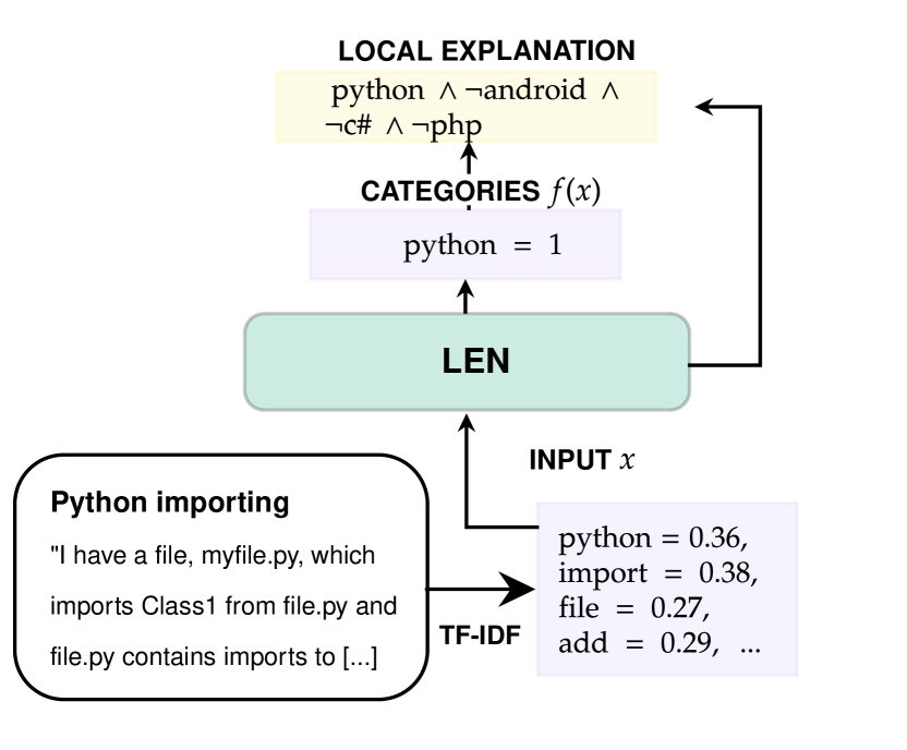
Figure 1: Example of LEN local explanations for a text predicted as ‘python’ tag.

LEN

The Logic Explained Network (Ciravegna et al., 2021) is a novel XAI architectural framework forming special kind of neural networks that are explainable-by-design. In particular, LENs impose architectural sparsity to provide explanations for a given classification task. Explanations are in the form of First-Order Logic (FOL) formulas approximating the behaviour of the whole network. A LEN $f$ is a mapping from $[0,1]^{d}$-valued input concepts to $r\geq 1$ output explanations, that can be used either to directly classify data and provide relevant explanations or to explain an existing black-box classifier. At test time, a prediction $f_{i}(x)=1$ is locally explained by the conjunction $\phi^{(i)}_{l}$ of the most relevant input features for the class $i\in\{1,\ldots,r\}$:

$$\text{LEN Local Exp.: }\phi_{l}^{(i)}(x)=\bigwedge_{\mathbf{x_{j}}\in\mathcal{A}^{(i)}}\mathbf{x_{j}}(x),$$ (1)

where $\mathbf{x_{j}}(x)$ is a logic predicate associated to the $j$-th input data and $\mathcal{A}^{(i)}$ is the set of relevant input features for the $i$-th task. Any $\mathbf{x_{j}}(x)$ can be either a positive $\mathbf{x_{j}}(x)$ or negative $\neg\mathbf{x_{j}}(x)$ literal, according to a given threshold, e.g. $\mathbf{x_{j}}(x)=[x_{j}>0.5]$. In this work, we consider the LEN proposed in Barbiero et al. (2022), where the set of important features $\mathcal{A}^{(i)}$ for task $i$ is defined as $\mathcal{A}^{(i)}=\{\mathbf{x_{j}}\ |\ 1\leq j\leq d,\ \alpha_{j}^{(i)}\geq 0.5\}$, where $\alpha_{j}^{(i)}$ is the importance score of the $j$-th feature, computed as the normalized softmax over the input weights $W$ connecting the $j$-th input to the first network layer $||W^{(i)}_{j}||_{1}$. Architectural sparsity is obtained by minimizing the entropy of the $\alpha$ distribution.

For global explanations, LENs consider the disjunction of the most important local explanations:

$$\text{LEN Global Exp.: }\phi_{g}^{(i)}=\bigvee_{\phi_{l}^{(i)}\in\mathcal{B}^{(i)}}\phi_{l}^{(i)},$$ (2)

where $\mathcal{B}^{(i)}$ collects the $k$-most frequent local explanations of the training set and is computed as $\mathcal{B}^{(i)}=\{\phi_{l}^{(i)}\in\arg\max_{\phi_{l}^{(i)}\in\Phi_{l}^{(i)}}^{k}\mu(\phi_{l}^{(i)})\}$, where we indicated with $\mu(\cdot)$ the frequency counting operator and with $\Phi_{l}^{(i)}$ the overall set of local explanations related to the $i$-th class. In addition to this, Ciravegna et al. (2021) employs a greedy strategy, gradually aggregating frequent local explanations only if they improve the validation accuracy.

3 LEN^p

3.1 Improving Local Explanation

The LEN algorithm for obtaining local explanations is not precise in determining the contribute of each feature. A close look at the extraction method shows that the $\alpha$ score only highlights the importance of a feature, without considering the type of contribution (either positive or negative) for the predicted class. As an example, consider an input text predicted as referring to C#. The LEN may have learned that the presence of the word C# leads to the tag prediction C# and so it has assigned a high importance value $\alpha_{\verb|C#|}^{(\verb|C#|)}$. However, sometimes we may not have the word C# in the text and still get the prediction to be C#. The algorithm proposed in (Barbiero et al., 2022) would extract a local explanation with the term $\neg\verb|C#|$, as shown in Figure 2. This is inaccurate because the absence of C# does not lead to prediction of the tag C#.

To improve the local explanations of LENs, we take the most important terms $\mathcal{A}^{(i)}$ and we divide them into two subsets – the good terms and the bad terms. The good terms are the ones that actually lead to the prediction. The bad terms are the ones despite which we get the given prediction. For each term, we decide whether it is good or bad by comparing the predicted probability of the tag with the current input and with a perturbed one (flipping term presence). If the prediction increases with the perturbation, the term is labelled as a bad term, otherwise it is considered a good term. Notice that the logic sign still comes from the input feature presence/absence. For ease, we only consider the conjunction of the good terms as the final explanation. Figure 2 shows the ability of LEN^p local explanation algorithm to correctly identify that the prediction is despite the absence of C#. Algorithm 1 in Appendix A, shows the pseudocode for the LEN^p local explanations.

We note that a similar algorithm is used in Anchors (Ribeiro et al., 2018). However, our approach can be more effective as we perturb and assess the importance of both the given input words and of the (important) absent ones. Indeed, Anchors formulae only report positive literals by inspecting the global behaviour of the model, while we also provide logic explanations with negative terms.

Figure 2: Sample local explanations using the original LEN strategy and the improved LEN^p strategy. The model has learned that C#, .NET in input leads to tag C# and have high importance.

Question	Which .NET collection should I use for adding multiple objects at once and getting notified?
Predicted Tags	C#
LEN explanation	$\neg$ C# $\wedge$ .NET
LENp explanation	.NET
	($\neg$ C# is a bad term, discarded)

3.2 Global Explanation

The greedy aggregation technique in Ciravegna et al. (2021) may not find an optimal solution. The time complexity of the original aggregation method is $O(k\times n)$, since they evaluate the validation accuracy of the global formula (for $n$ samples) while aggregating the $k$ local explanations. However, when we aggregate a small number of local explanations, i.e. $k$ is small, we can afford a more effective but slower solution. Straightforwardly, we compute the disjunctions of all the possible combinations of local explanations (power set), incurring in a $O(2^{k}\times n)$ time complexity, but finding an optimal solution, i.e. the one reaching the higher validation accuracy. Note that to keep the explanations short and easy to interpret, normally $k$ is very small, between $3$ and $10$. In Appendix A, Algorithm 2 shows the improved LEN^p aggregation method.

4 Experiments

In the experimental section, we show that (i) LEN^p improves LEN explanations and provides better explanations than LIME in terms of faithfulness, sensitivity and capability to detect biased-model (Section 4.1) and (ii) a human study confirms this result, in particular when considering the global explanation (Section 4.2). Furthermore, in Appendix B, we confirm that LENs achieve competitive performance when employed as explainable-by-design classifier w.r.t. black-box models. Appendix C contains experimental details.

4.1 Explanation Comparison

To assess the quality of the explanations of the proposed method (LEN^p), we compared it with the original LEN algorithm (LEN), a version of LIME with discretized input (LIME (D)), and a version of LIME with non-discretized input (LIME (ND)).

We compare the different strategies by explaining a common black-box Random Forest model. Due to the high computational complexity required to explain each of the $\sim$ 15K tags (reduced from the initial 37K tags, after retaining only important questions), we compare the local explanations overs three tags only, namely “C#”, “Java” and “Python”. The hyperparameters of each method were chosen to get the best results while keeping the computational time to be at most 15 minutes.

LEN^p provides faithful explanations

The faithfulness of an explanation to a model refers to how accurate the explanation is in describing the model decision process. To evaluate the faithfulness, we use the Area Under the Most Relevant First perturbation Curve (AUC-MoRF). The lesser the value of AUC-MoRF, the more faithful is the explanation to the model. We calculate the AUC-MoRF for each strategy, considering the local explanation over 100 samples.

Table 1: Average AUC-MoRF with 95% confidence interval. The lower, the better.

Explanation	AUC-MoRF
Strategy
LEN	$0.4985\pm 0.0283$
LENp	$0.0489\pm 0.0117$
LIME (D)	$0.4413\pm 0.0171$
LIME (ND)	$0.3919\pm 0.0159$

Table 2: Average Max-Sensitivity with 95% confidence interval. The lower, the better.

Explanation	Max-Sensitivity
Strategy
LEN	$0.0000\pm 0.0000$
LENp	$0.0000\pm 0.0000$
LIME (D)	$1.4031\pm 0.1482$
LIME (ND)	$1.3978\pm 0.0467$

Table 3: Capability to detect biased-model. We report the percentage of times the compared explanation algorithm detect the use of noisy features in biased model in two experimental settings.

Explanation	S1	S2
Strategy
LENp	$80\%$	$95\%$
LEN	$10\%$	$55\%$
SP-LIME (D)	$05\%$	$25\%$
SP-LIME (ND)	$00\%$	$00\%$

Table 1 reports the average AUC-MoRF for the different explanation strategies. The LEN^p provides more faithful explanations than all the competitors by a considerable margin. On the contrary, the original LEN explanations are slightly less faithful than LIME (D) and LIME (ND).

LEN^p explanations are robust to perturbations

The sensitivity of an explanation refers to the tendency of the explanation to change with minor changes to the input. In general, a robust explanation is not affected by small random perturbations, since we expect similar inputs to have similar explanations. Therefore, low sensitivity values are desirable and we measure the Max-Sensitivity. For more details about the metric, please refer to Appendix D. Table 2 report the average Max-Sensitivity evaluated over 100 randomly selected inputs and performing 10 random perturbations $x^{\star}$ per input $x$, with maximum radius $\epsilon=||x-x^{\star}||_{\infty}=0.02$. We see that explanations from both LEN and LEN^p have $0.0$ Max-Sensitivity, i.e., they remain unchanged by all minor perturbations to the input, greatly outperforming the explanations from LIME. This is expected because LEN trains the model once over all the training data and tries to act as a surrogate model; there is no retraining for a new local explanation. On the other hand, LIME trains a new linear model for each local explanation and only try to mimic the explained model on the predictions near the given input. Clearly, by employing larger perturbation of the input, LEN explanations would also change.

LEN^p is capable to detect biased-model

The presence of noisy features in the training data may drive a model to unforeseeable prediction on clean data at test time. For this reason, it is very important to detect them before releasing the model. A way to detect biases is to compute the global explanation of a model and check whether the explanation is consistent with the domain knowledge. To this aim, it is very important to employ a powerful explanation algorithm that may be capable to detect the bias. To evaluate this capability, we trained a model with the explicit goal of making it biased. In the training data, we added noisy features with a high correlation with certain tags, so that the model learns to associate the noisy features with the tag. At test time, these features are added randomly, i.e. they act like noise. We run these experiments in two settings, S1 and S2, varying the amount of bias towards the noisy features. This is done by increasing the bias of the noisy features in training data from 30% of training data in S1 to 35% in S2, and by ensuring a higher difference in test and validation scores in S2.

Table 3 reports the percentage of times we are able to detect the use of noisy features using the global explanations from the different strategies. LEN^p shows more utility than all the competitors by a large margin. The results have been averaged over 20 executions in this setting.

4.2 Human Survey

We carried out a human survey to compare the ease of understanding and the utility of the explanations obtained by LIME and LENs. The human survey was approved by the ethics committee and the questions do not record personal information. The survey was shared with students and researchers over different universities and filled by $26$ respondents, $13$ with experience in Machine Learning, $10$ in Computer Science and $3$ in neither. The survey is attached in Appendix E. Figure 3 report the ease of using the explanations for the different task.

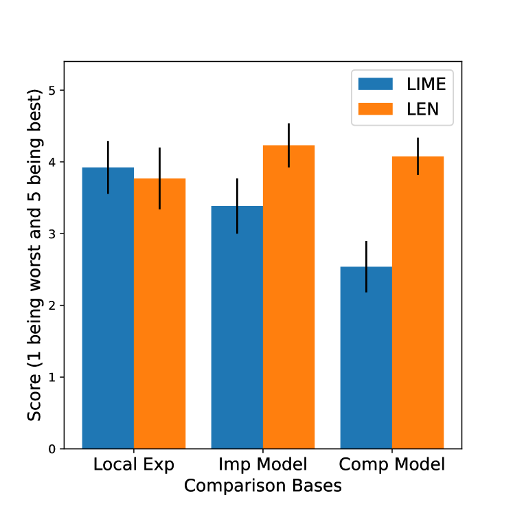
Figure 3: Survey rating results with $95\%$ confidence intervals

Table 4: Survey tasks results

Quantity Measured	LIME	LEN
Respondents able to identify the feature to ignore to improve the classifier	$61.5\%$	$84.6\%$
Respondents able to identify the more general classifier	$50.0\%$	$73.1\%$

LEN^p explanations are easily interpretable

First, the survey presents the respondents a sample input with the related prediction and the explanations from LIME and LEN^p. It then asks the respondents to rate the ease of understanding these local explanations. The first column of Figure 3 suggests that the local explanations from LIME and LEN^p are almost equally easily understandable since the $95\%$ confidence intervals have a high overlap (with LIME having a slightly higher mean).

LEN^p enable users to improve a classifier

This section aims to establish the usefulness of the explainers in getting a more general classifier through feature engineering. To this aim, we trained a radial basis function (RBF) SVM to mistakenly learn to associate the feature ‘add’ with the C# tag. This was done by perturbing the training data and ensuring a wide difference in the validation and testing scores. We asked respondents to identify the input feature which does not allow the model to generalize well, by inspecting the global explanation of SP-LIME and LEN^p. They were also asked to rate the ease of using the explanations for this purpose. As shown in Table 4 first row, only 61.5% respondents were able to identify the term ‘add’ as the feature to ignore while using LIME explanations, as opposed to LEN^p 84.6%. In addition, in Figure 3 second column, respondents found LEN^p easier to use for improving the classifier.

LEN^p allows identifying the best classifiers

Finally, we evaluated whether users can choose a classifier that generalizes better than the other, by only checking again the global explanations of the two classifiers. To this aim, we trained two RBF SVMs classifiers on different training data (the second one with some noise added). As reported in Table 4, second row, 73.1% respondents were able to identify the more general classifier using LEN^p as opposed to LIME 50%. Moreover, the third column of Figure 3 shows that the global explanations from LEN^p make the comparison much easier than those from SP-LIME.

5 Conclusion

This paper proposes LEN^p, an improved version of LENs whose results clearly show that LEN^p explanations outperform both LEN and LIME on different metrics (sensitivity and faithfulness). Moreover, a user study demonstrated that the logic explanations are more useful than the importance vector and provide a better user-experience (particularly on global explanation). This has wide-ranging impact, as LIME is a popular strategy used in various fields (e.g., Gramegna and Giudici (2021) and Visani et al. (2020)).

6 Limitations

Regarding the aggregation of local explanations, the proposed algorithm can be intractable in case $k$ is not small. To alleviate this issue, we are working on a selective algorithm to automatically filter out the local explanations that are less useful for the task. Furthermore, since LENs require concepts as input, we did not consider models taking sequential input in this work. In future work, we will test the explanation of the proposed model when explaining sequential models, making use of concept extraction from sequential models, like the work done by Dalvi et al. (2022). The backbone itself of the LEN is an MLP architecture, but it might be interesting to devise a LEN-version of an RNN or a Transformer model. The human survey does represent the target users, as the topic experts for StackOverflow questions are computer scientists. However, in future work, to better represent the population of possible users, we aim at expanding the portion of not expert in neither Machine learning nor Computer Science. Finally, the paper only compares LEN and LIME explanation on one dataset, but it might be interesting to broaden the comparison to include SHAP, LORE and Anchors, while considering a variety of datasets.

Appendix A Algorithms

In this section, we report the local and global explanation methods from LEN^p. In particular, Algorithm 1 reports the pseudocode for improving the local explanations from the LEN, while Algorithm 2 reports the optimal aggregation mechanism proposed in this paper.

1 Function local_explanation($model$, $x$, $target\_class$):

2       $exp\leftarrow$ Original LEN local explanation

3       $org\_pred\leftarrow$ $model(x)$

4       $good\_terms,bad\_terms\leftarrow[\,],[\,]$

5       forall $term\in$ exp do

6             $x^{\prime}\leftarrow$ Clone $x$ with $term$ flipped

7             $pert\_pred\leftarrow model(x^{\prime})$

8             if $org\_pred\leq pert\_pred$ then

9                   $bad\_terms$.append($term$)

10                  

11            else

12                   $good\_terms$.append($term$)

13                  

14             end if

15            

16       end forall

17      return Conjunction($good\_terms$)

18      

19

Algorithm 1 LEN^p Local Explanation

1 Function aggregate_explanations( $topk\_explanations$):

2       $all\_comb\leftarrow$ PowerSet($topk\_explanations$)

3       forall $exps\in all\_comb$ do

4             $cur\_exp\leftarrow\bigvee exp\text{ for }exp\in exps$

5             $accuracy\leftarrow$ Calculate accuracy of $cur\_exp$ on $validation\_data$

6             if $accuracy>best\_acc$ then

7                   $best\_exp\leftarrow cur\_exp$

8                   $best\_acc\leftarrow accuracy$

9                  

10             end if

11            

12       end forall

13      return $best\_exp$

14      

15

Algorithm 2 LEN^p global explanation

Appendix B Model Evaluation

In this section, we employ the LEN directly as a classifier, to assess the performance drop required to employ an explainable-by-design network instead of a black-box one.

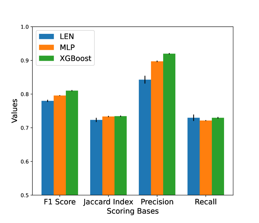
Figure 4: Evaluation Values for the different models

Figure 4 compares the predicting performance of the LEN with an MLP and an XGBoost, two black-box models, in terms of F1 Score, Jaccard Index, Precision and Recall. Results are averaged 10 times over different test-train splits and model initializations. We also report the $95\%$ confidence intervals.

We observe that XGBoost performs better than both the LEN model and the MLP in all metrics. We can also appreciate that the LEN proposed in (Barbiero et al., 2022) only slightly decreases the performance w.r.t. using almost identical MLP. A higher difference was expected, as in general there exists a trade-off between the model explainability and its performance (Barredo Arrieta et al., 2019). These results indicate that the performance of LEN is good/comparable enough to consider replacing outperforming black-box models to gain higher interpretability.

Appendix C Experimental details

Hardware

All experiments were run on a machine equipped with an Intel i7-8750H CPU, an NVIDIA GTX 1070 GPU and 16 GB of RAM.

Hyper-parameters

The selection was done with a grid search alongside, to maintain fairness in comparison, a constraint on the time required to obtain explanations.

Simulation Experiments

The details about the different settings, S1 and S2, of the experiment described in Section 4.1, is as follows: In each run of S1, we add 2 noisy features. In training data, each noisy features is added with a 30% probability of being added to inputs of tag C# and 5% probability to the other tags. In testing data, it is added uniformly added to all tags with 5% probability. Bias is ensured by having a threshold difference of 0.03 between the test and validation F1 scores.

S2 follows similarly, where we add 2 noisy features, but increase the probability of adding them to inputs of tag C# in training data from 30% to 35%. The threshold difference of F1 scores is also increased to 0.05. This is done to get a model that uses the noisy features with higher importance than that we get with setting S1.

Appendix D Evaluation of Trust in Explanations

In general, trust in the explanations refers to reliability of the explanations. In this paper, we used two metrics to measure this trust in the explanations, the AUC-MoRF and the Max-Sensitivity, for which we reported the details below.

Area Under the Most Relevant First Perturbation Curve

Area Under the Most Relevant First Perturbation Curve (AUC-MoRF) (Kakogeorgiou and Karantzalos, 2021) is a metric based on the MoRF perturbation curve as proposed by Samek et al. (Samek et al., 2017). MoRF curve is the plot of prediction from model versus the number of features perturbed, where the features are perturbed in a most relevant first order. Thus, AUC-MoRF can be defined as:

$$\text{AUC}_{\text{MoRF}}(\Phi,f,x)=\sum_{k=2}^{D}\frac{f(y^{(k-1)})+f(y^{(k)})}{2}$$ (3)

Here $f$ is the model being explained, $x$ is an input vector, $\Phi$ is an explanation method, $D$ is the number of input features and $y^{(k)}$ is the input vector after the $k^{\text{th}}$ MoRF perturbation. MoRF perturbations are defined recursively as below:

$$\begin{split}y^{(0)}&=x\\ \forall 1\leq k\leq D:y^{(k)}&=g(y^{(k-1)},r_{k}\end{split}$$ (4)

Here $g$ is a function that takes a vector and an index, and perturbs the given vector at the given index, and $[r_{1},r_{2},\ldots,r_{D}]$ are the indices of the input features sorted in descending order of their relevance, as determined by the explanation $\Phi$.

In our evaluation, we normalize the AUC-MoRF values to be in the $[0,1]$ range, by dividing the values by $D-1$ when $D>1$. So, the final formula used looks like:

$$\begin{split}\text{Normalized}&\text{ AUC}_{\text{MoRF}}(\Phi,f,x)=\\ =&\frac{1}{(D-1)}\sum_{k=2}^{D}\frac{f(y^{(k-1)})+f(y^{(k)})}{2}\end{split}$$ (5)

A lesser value of AUC-MoRF means a more faithful explanation, and thus a more trustworthy explanation.

Max-Sensitivity

Sensitivity of an explanation measures the proneness of the explanation to be affected by insignificant perturbations to the input. Max-Sensitivity is a metric due to Yeh et al. (Yeh et al., 2019) which is defined as below:

$$\begin{split}\text{SENS}_{\text{MAX}}&(\Phi,f,x,r)=\\ &=\max_{\left\lVert y-x\right\rVert\leq r}\left\lVert\Phi(f,y)-\Phi(f,x)\right\rVert\end{split}$$ (6)

Here $f$ is the model being explained, $x$ is an input vector, $y$ is the input vector with some perturbations, $r$ is the max perturbation radius, and $\Phi$ is an explanation method, which takes a model and input vector and gives the explanation.

The lesser the value of this metric, the lesser is the explanation prone to minor perturbations in the input, and so more is our trust in the explanation.

Appendix E Human Survey

In the following pages, we report a compressed copy of the human survey for which we reported the results in Section 4.2.

In the survey section where we aim to establish the usefulness of the explainers in getting a more general classifier, we train a radial basis function (RBF) SVM to mistakenly learn to associate the feature ‘add’ with the C# tag. This was done by randomly adding (with 50% probability) “add” only to the training data labeled with the C# tag. RBF-SVM was trained on this perturbed data, getting a 6% smaller Jaccard Index validation score than the training one. This difference confirmed that the model mistakenly learned to associate “add” with C# tag.

See pages 1-6 of survey_2.pdf

References

- Adadi and Berrada (2018) Amina Adadi and Mohammed Berrada. 2018. Peeking inside the black-box: a survey on explainable artificial intelligence (xai). IEEE access, 6:52138–52160.
- Barbiero et al. (2022) Pietro Barbiero, Gabriele Ciravegna, Francesco Giannini, Pietro Lió, Marco Gori, and Stefano Melacci. 2022. Entropy-based logic explanations of neural networks. In Proceedings of the AAAI Conference on Artificial Intelligence, volume 36, pages 6046–6054.
- Barredo Arrieta et al. (2019) Alejandro Barredo Arrieta, Natalia Diaz Rodriguez, Javier Del Ser, Adrien Bennetot, Siham Tabik, Alberto Barbado González, Salvador Garcia, Sergio Gil-Lopez, Daniel Molina, V. Richard Benjamins, Raja Chatila, and Francisco Herrera. 2019. Explainable artificial intelligence (xai): Concepts, taxonomies, opportunities and challenges toward responsible ai. Information Fusion, 58.
- Ciravegna et al. (2021) Gabriele Ciravegna, Pietro Barbiero, Francesco Giannini, Marco Gori, Pietro Lió, Marco Maggini, and Stefano Melacci. 2021. Logic explained networks. arXiv preprint arXiv:2108.05149.
- Dalvi et al. (2022) Fahim Dalvi, Abdul Rafae Khan, Firoj Alam, Nadir Durrani, Jia Xu, and Hassan Sajjad. 2022. Discovering latent concepts learned in bert.
- Gramegna and Giudici (2021) Alex Gramegna and Paolo Giudici. 2021. Shap and lime: An evaluation of discriminative power in credit risk. Frontiers in Artificial Intelligence, 4.
- Guidotti et al. (2018) Riccardo Guidotti, Anna Monreale, Salvatore Ruggieri, Dino Pedreschi, Franco Turini, and Fosca Giannotti. 2018. Local rule-based explanations of black box decision systems. arXiv preprint arXiv:1805.10820.
- Kakogeorgiou and Karantzalos (2021) Ioannis Kakogeorgiou and Konstantinos Karantzalos. 2021. Evaluating explainable artificial intelligence methods for multi-label deep learning classification tasks in remote sensing.
- LeCun et al. (2015) Yann LeCun, Yoshua Bengio, and Geoffrey Hinton. 2015. Deep learning. nature, 521(7553):436–444.
- Lundberg and Lee (2017) Scott M Lundberg and Su-In Lee. 2017. A unified approach to interpreting model predictions. In I. Guyon, U. V. Luxburg, S. Bengio, H. Wallach, R. Fergus, S. Vishwanathan, and R. Garnett, editors, Advances in Neural Information Processing Systems 30, pages 4765–4774. Curran Associates, Inc.
- Minaee et al. (2020) Shervin Minaee, Nal Kalchbrenner, Erik Cambria, Narjes Nikzad, Meysam Chenaghlu, and Jianfeng Gao. 2020. Deep learning based text classification: A comprehensive review.
- Overflow (2019) Stack Overflow. 2019. Stacksample: 10% of stack overflow q&a.
- Ribeiro et al. (2016) Marco Tulio Ribeiro, Sameer Singh, and Carlos Guestrin. 2016. "why should I trust you?": Explaining the predictions of any classifier. In Proceedings of the 22nd ACM SIGKDD International Conference on Knowledge Discovery and Data Mining, San Francisco, CA, USA, August 13-17, 2016, pages 1135–1144.
- Ribeiro et al. (2018) Marco Tulio Ribeiro, Sameer Singh, and Carlos Guestrin. 2018. Anchors: High-precision model-agnostic explanations. In Proceedings of the AAAI conference on artificial intelligence, volume 32.
- Samek et al. (2017) Wojciech Samek, Alexander Binder, Gregoire Montavon, Sebastian Lapuschkin, and Klaus-Robert Müller. 2017. Evaluating the visualization of what a deep neural network has learned. IEEE Transactions on Neural Networks and Learning Systems, 28:2660–2673.
- Selbst and Powles (2017) Andrew D Selbst and Julia Powles. 2017. Meaningful information and the right to explanation. International Data Privacy Law, 7(4):233–242.
- Vaswani et al. (2017) Ashish Vaswani, Noam Shazeer, Niki Parmar, Jakob Uszkoreit, Llion Jones, Aidan N Gomez, Łukasz Kaiser, and Illia Polosukhin. 2017. Attention is all you need. Advances in neural information processing systems, 30.
- Visani et al. (2020) Giorgio Visani, Enrico Bagli, and Federico Chesani. 2020. Optilime: Optimized lime explanations for diagnostic computer algorithms.
- Yeh et al. (2019) Chih-Kuan Yeh, Cheng-Yu Hsieh, Arun Suggala, David I Inouye, and Pradeep K Ravikumar. 2019. On the (in)fidelity and sensitivity of explanations. In Advances in Neural Information Processing Systems, volume 32. Curran Associates, Inc.