Abstract

Bayesian inference with nested sampling requires a likelihood-restricted prior sampling method, which draws samples from the prior distribution that exceed a likelihood threshold. For high-dimensional problems, Markov Chain Monte Carlo derivatives have been proposed. We numerically study ten algorithms based on slice sampling, hit-and-run and differential evolution algorithms in ellipsoidal, non-ellipsoidal and non-convex problems from 2 to 100 dimensions. Mixing capabilities are evaluated with the nested sampling shrinkage test. This makes our results valid independent of how heavy-tailed the posteriors are. Given the same number of steps, slice sampling is outperformed by hit-and-run and whitened slice sampling, while whitened hit-and-run does not provide as good results. Proposing along differential vectors of live point pairs also leads to the highest efficiencies, and appears promising for multi-modal problems. The tested proposals are implemented in the UltraNest nested sampling package, enabling efficient low and high-dimensional inference of a large class of practical inference problems relevant to astronomy, cosmology, particle physics and astronomy.

1 1 0 https://doi.org/

1 Introduction

The nested sampling Monte Carlo algorithm (proposed by (Skilling, 2004) and recently reviewed in (Ashton et al., 2022) and (Buchner, 2021)) enables Bayesian inference by estimating the posterior and its integral. A population of $K$ live points are sampled randomly from the prior. Then, the lowest likelihood point is discarded, and a new live point is sampled from the prior under the constraint that its likelihood must by higher than the discarded point. This is iteratively repeated in nested sampling. The likelihood-restricted prior sampling (LRPS), if unbiased, causes the likelihoods of discarded points to have interesting properties. In particular, the fraction of prior mass below the likelihood threshold is approximately $1/K$. The recursive estimation of prior mass discarded, together with the sampled likelihood, allows nested sampling to perform the integration.

The first LRPS algorithms proposed were adaptations of Markov Chain Monte Carlo (MCMC) variants. For simplicity, here we assume that the parameters have been parameterized so that the prior probability density is uniform. Then, in a Gaussian Metropolis MCMC started from a randomly chosen live point a random nearby point would be proposed. If the likelihood there exceeds the current threshold, it replaces the starting point for the next iteration. This procedure is repeated $N_{\mathrm{steps}}$ times, after which the final point is considered a sufficiently independent prior sample. Since the value of the likelihood is not considered further, this pursues a purely geometric random walk. The class of such step sampler algorithms (Buchner, 2014) includes slice sampling (Neal, 2003), first proposed for LRPS by (Jasa and Xiang, 2005). In section §2.4 we describe ten members of a larger family of algorithms which includes slice sampling. These algorithms are popular because no additional parameters that influence its outcome need to be chosen, making applications to a wide variety of problems robust. When the dimensionality $d$ of the inference problem is high ($d\gg 20$), i.e., the fitted model has many parameters, such step samplers tend to outperform rejection sampling-based algorithms (see (Buchner, 2021) for a survey).

Given a inference problem with $d$ parameters, choosing a LRPS method and its parameters is not trivial. Detecting biased LRPS is a question of on-going research (e.g., (Buchner, 2014; Higson et al., 2019; Fowlie et al., 2020)), and we give our definition of acceptable LRPS quality in §2.1. Our procedure for calibrating $N_{\mathrm{steps}}$ is described in §2.3. The test problems are listed in §2.2 and the LRPS methods described in §2.4. The evaluation results of the mixing behaviour of the various LRPS methods is presented in §3.1, and discussed in §4.

2 Materials and Methods

2.1 Distinguishing good and bad LRPS performance

How can we judge that one method performs better than another, or even acceptably well? We could run NS on example inference problems and analyse the produced posterior and integral. While this may be very realistic, the results would be limited to the geometry and likelihood slopes of that particular inference problem, leaving generalization to different data or models unclear. It is also difficult to define an objective criterion on whether the integral and posterior approximation is acceptable, in addition to the requirement that the true result is available for comparison. Alternative to such a “in vivo” test, we could explore the geometric mixing behaviour in isolation (“in vitro”). For example, from initial samples concentrated in a small ball, we could measure the time until samples have converge to true geometry. Here, the information gain could measure the quality, but thresholds are also unclear. Additionally, in NS the situation is not static, rather a sequence of similar geometries is explored with ever-shrinking size. To address the shortcomings listed above, we instead adopt a verification test built for NS that is already familiar.

The shrinkage test was presented by (Buchner, 2014). In problems where the volume enclosed at a likelihood threshold, $V({\cal L})$, can be computed, the shrinkage test analyses the volume ratio distribution $V_{i+1}/V_{i}$ of a sequence of discarded samples produced by NS with a LRPS. This measures the critical issue of interest, namely, whether the shrinkage is passed to NS correctly (following the expected beta distribution) by an unbiased LRPS.

The shrinkage test can flag problematic LRPS methods. We collect shrinkage samples for $25\times K$ LRPS iterations, with $K=400$ live points. Given these samples from $10,000$ iterations, configurations are rejected if the shrinkage KS test gives a p-value below 0.01. We consider a configuration the combination of a LRPS method together with its hyperparameters. Additionally, if any iteration had no movement (live point is stuck), the configuration is also rejected. The LRPS is started with live points drawn perfectly from the geometry, and the first $3\times K$ iterations are not included in sample collection to allow the LRPS method to warm up and calibrate.

On real inference problems, troublesome situations may occur at some arbitrary iteration and persist for some arbitrary length, both of which modulate the impact on evidence and posterior estimation. The shrinkage test is independent of this and thus provides conservative results. With NS applications typically requiring several tens of thousands iterations, our detections of deviations provide lower limits. Importantly, the shrinkage test results are independent of the likelihood slope and are therefore generalizable. Only the geometry of the likelihood contours are important, regardless of how informative the posterior is, whether there are phase transitions, etc. While the requirement that $V({\cal L})$ can be computed analytically may seem restrictive, this is possible for difficult geometries (§2.2), including ellipsoidal, multi-ellipsoidal, convex and non-convex problems. We seek LRPS methods that behave robustly across such situations.

2.2 Geometries considered

Likelihood contours can be classified into convex or non-convex, depending on whether the linear interpolation between two points within the restricted prior is also inside. A sub-class of the convex geometries are ellipsoidal contours, arising from Gaussian or other ellipsoidal posterior distributions. This classification can also be considered locally. Different information gain per parameter influences how the contour changes shape.

Our goal here is to span the space of geometries across dimensionality, while simultaneously avoiding excessive computational cost. Therefore, we sparsely sample the problem space of geometries with six setups. This includes (1) as a ellipsoidal problem a correlated Gaussian with covariance $\Sigma_{ij}=0.95$ and a unit diagonal, in 16 and 100 dimensions, (2) as a difficult convex problem the hyperpyramid with log-likelihood $\log{\cal L}=\max_{i}\{|x|\}$ in four and 16 dimensions, and (3) as a non-convex problem the Gaussian shell problem (Feroz and Hobson, 2008) $\log{\cal L}=-((||x-0.5||^{2}-0.4^{2})/0.004)^{2}$ in two and eight dimensions. The former two are self-similar across iterations, while the last is not, with the shell thickness becoming thinner with increased iteration. To avoid entering extreme situations infrequent in real applications, short runs of length $3000$ ($d=2$) and $6000$ iterations ($d=8$) were performed with different seeds, and repeated until the desired number of samples were collected.

The scope sampled by these geometries is limited, and does not capture all real-world situations of interest. The scope of this work is to develop a methodology to evaluate LRPS behaviour and to discard configurations that are already showing problematic behaviour in these simple geometries. However, there are some relevancies. For example, posteriors often are Gaussians away from the borders, which is approximated by (1). Configuration (2) approximates when the data impose upper limits on each parameter independently. Non-linear banana degeneracies are a sub-set of (3). Multi-modal problems are left for future work. However, we can extrapolate in limited way: Methods that only consider local instead of global live point correlations may be unimpacted by inter-mode structure, and thus our results may hold for these. To emphasize, some reasonable situations are considered here in-vitro to place some limits on in-vivo behaviour, but we do not aim to consider the most difficult case conceivable.

2.3 Calibrating the number of steps

To find the $N_{\mathrm{steps}}$ required to sample the geometry correctly, a run as described above with $N_{\mathrm{steps}}=1$ is performed. Upon rejection, $N_{\mathrm{steps}}$ is doubled until success. Since we want a lower limit $N_{steps}(d)$ usable by practitioners, and because this should be a monotonically increasing function, an improvement for computational efficiency can be made: If the test problems are ordered by $d$, then the next problem does not need to be tested on $N_{\mathrm{steps}}$ that already failed a previous problem. So we run the problems in order of $d$ and initialize the search for $N_{\mathrm{steps}}$ at the value that was acceptable for the previous problem. This automatically finds a conservative $N_{steps}(d)$ curve across the different problems.

2.4 LRPS methods considered

Multiple algorithms are considered. Within a single step, they have similar behaviour, which we describe first. From a starting point $x$, a direction $v$ is chosen. To sample a point on the slice $y(t)=x+t\times v$, with $t$ uniformly sampled, bounds on $t$ first need to be found. Given a guess length $L$, initially $L=1$, the point at $t=L$, $t=2L$ etc. is tested until the point lies outside the restricted prior, $t=2^{i}L$. The same is repeated for negative $t$ values. Then, $t$ can be uniformly sampled between $t_{-}$ and $t_{+}$. If the point $y(t)$ is rejected, subsequent tries can set $t_{-}=t$ (if $t$ is negative) or $t_{+}=t$ (if $t$ is positive). This is akin to bisection and assumes convexity (Neal, 2003). When the $y(t)$ point is accepted, the sampling is restarted from there. This is done $N_{\mathrm{steps}}$ times. The number of model evaluations per NS iteration is therefore $N_{\mathrm{steps}}\times(i_{+}+i_{-}+j)$, where the $i$ stepping out iterations and $j$ bisection steps, are subject to the constraint behaviour and the direction proposal. The guess length $L$ is increased by $10\%$ if $i_{+}+i_{-}>0$, or decreased by 10% otherwise.

We consider ten algorithms, which differ in their direction proposal. The algorithm variants are:

1. cube-slice: In slice sampling, one parameter is randomly chosen as the slice axis (Neal, 2003).

2. region-slice: Whitened slice sampling, randomly choosing a principal axis based on the estimated covariance matrix.

3. region-seq-slice: Whitened slice sampling, iteratively choosing a principal axis (Speagle, 2020).

4. cube-harm: Hit-and-run sampling choses a randomly chosen direction from the unit sphere ((Turchin, 1971); combined with slice bisection: (Kiatsupaibul et al., 2011)).

5. region-harm: Whitened hit-and-run sampling by randomly choosing a ball direction using the sample covariance.

6. cube-ortho-harm and

7. region-ortho-harm are the same as cube-harm and region-harm, but prepare a sequence of $d$ proposals that are made orthogonal by Gram-Schmidt, then use them in order. This is similar to the PolyChord (Handley et al., 2015) implementation.

8. de-harm: Differential evolution (randomly choose pair of live points and use their differential vector) (Ter Braak, 2006)

9. de1: same as de-harm, but set the difference in all but one, randomly chosen dimension to zero. This is very similar to cube-slice, but scales the direction using the distance between points.

10. de-mix: randomly choose between de-harm and region-slice at each step with equal probability.

The phase from proposing a slice until acceptance of a point on that slice is considered a single slice sampling step for counting to $N_{\mathrm{steps}}$. This is also the case for methods where subsequent proposals are prepared together (e.g., region-seq-slice, cube-ortho-harm, region-ortho-harm). Some algorithms take advantage of the sample covariance matrix estimated from the live points, and its principle axis, to whiten the problem space. We estimate the covariance matrix every $K/5$ nested sampling iterations, i.e., when the space has shrunk to $(1-1/K)^{K/5}\approx 80\%$.

Detailed balance is satisfied by the cube-* and de-* methods. When whitening is computed from the live points, detailed balance is not retained. Since detailed balance is a sufficient but not a necessary condition of the Metropolis proposal, this may or may not lead to convergence issues. The shrinkage test should indicate this.

3 Results

3.1 Calibration results

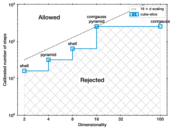
Figure 1: Calibration for the slice sampler (cube-slice).

To start, Figure 1 presents the calibration results for the cube-slice method. The $N_{\mathrm{steps}}$ needed for each problem is shown by the blue curve. In this case, the $N_{\mathrm{steps}}$ needed to be doubled or quadrupled for all but the last increase in dimensionality. Configurations to the bottom right of this curve are rejected, because biases in the shrinkage distributions were detected. Configurations in the upper left including the blue squares are still allowed, but may be problematic in geometries other than the ones considered here. The dotted black line shows the minimal scaling law that avoids the rejected configuration space.

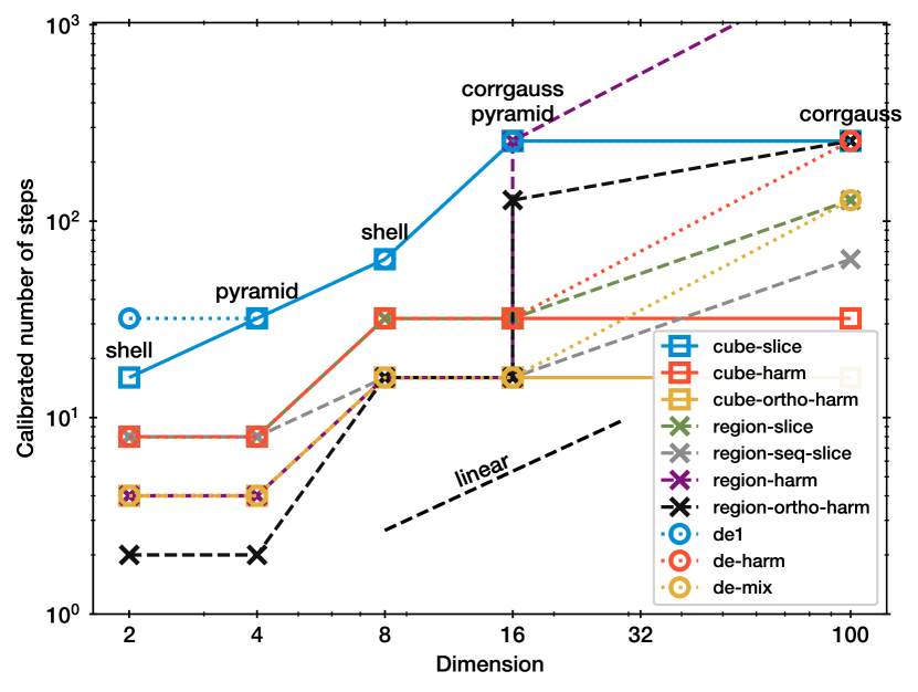
Figure 2: Calibration of all samplers.

Next, Figure 2 present the same calibration, but now for all step samplers. In general, all curves show an approximately linear increase with $d$, although with different normalisations.

de1 performs the same as cube-slice (blue circles with dotted curve and blue rectangles with solid curve). This is expected, because the methods are identical except for the proposed length step. It suggests our experimental setup gives reproducible results, even though the KS threshold has some randomness.

Table 1: Minimum scaling factor for a linear calibration $N_{\mathrm{steps}}=k\times d$. With the efficiency $\epsilon$ defined as number of model evaluations per iteration, the last column reports the lowest observed dimension-corrected efficiency $\epsilon\times d$.

Sampler	Factor $k$	Efficiency %
cube-slice	16	0.32
cube-harm	4	1.19
cube-ortho-harm	2	2.32
region-slice	4	1.16
region-seq-slice	4	1.69
region-harm	>16	–
region-ortho-harm	8	1.42
de1	16	0.43
de-harm	4	1.15
de-mix	2	2.33

For the 100d problem, region-harm did not converge even for $N_{\mathrm{steps}}>1024$, and is set to a arbitrary high value in this plot. The whitened hit-and-run methods (region-harm, region-ortho-harm) need the most steps, together with the de1. Only cube-harm needs few steps even in high-d. The calibrated scaling factors for each method are listed in Table 1.

Now that all methods are calibrated to perform correctly, we can compare their efficiency in a fair way. This is not the same as the number of steps, because the number of stepping-out iterations may differ.

3.2 Computational cost scaling with dimension

Figure 3: Calibration for slice sampler. and scaling.

Figure 3 presents the efficiency of each method. Specifically, this is the average number of model evaluations per NS iteration for the $N_{\mathrm{steps}}$ configuration where the shrinkage test indicates adequate performance (Figure 2). Overall, all curves in Figure 3 show approximately a $1/d$ behaviour. There is substantial vertical scatter, indicating that the efficiency is diverse across the methods and also dependant on problem. For example, the efficiency is generally higher for the pyramid geometry than for the more difficult shell.

4 Discussion

Methods can now be compared by the relative position of the curves in Figure 3. Slice sampling (blue squares) is the most inefficient among the considered methods. The single-parameter differential proposal (blue circle) has marginally improved the efficiency. Hit-and-run Monte Carlo (red squares) is more than twice as efficient as these. Orthogonalisation helps further (yellow squares). The differential proposal (de-harm) has comparable performance to these, with slightly better behaviour at lower $d$ than at high $d$.

The results from the whitened proposals (region-*) are diverse. To inform the discussion of these results, two opposing insights seem relevant. Firstly, whitening a space, or more accurately adjusting the proposal to the distribution sampled is a common MCMC technique to improve the proposal efficiency. For example, in a highly correlated Gaussian, sampling along one axis, then another will diffuse only short distances, while sampling along the principal axis generates distant jumps. This may be the interpretation for the poor performance of the cube-slice sampler (blue curve in Figure 3), relative to the region-slice (green crosses). A similar effect could be that picking the same axis twice may lead to unnecessary reversals. However, our results show efficiency worsens when the directions are sampled sequentially (region-seq-slice; gray crosses) instead of randomly (region-slice; green crosses).

Secondly, if the adaptation is computed from the live points, an iterative bias could be induced. Indeed, it is usually recommended to perform a warm-up or burn-in step which adjust the proposal, before a sampling phase where the proposal is fixed and the samples are trusted. (Huijser et al., 2015) observed that in the affine-invariant ensemble sampler (Goodman and Weare, 2010), which uses differential vectors from one half of the live points to update the other half of live points, the iterative updating can lead to a collapse onto a sub-space and hinder convergence to the true distribution at high dimension. Here we observe that while region-slice performs efficiently, and cube-harm performs efficiently, region-harm (purple crosses) performs very poorly at $d>16$. This may be a similar self-enforcing behaviour. The orthogonalisation of region-harm (black crosses) helps, but requires still a high number of steps at high dimension. It is interesting that cube-harm does not show this behaviour. From this, we can therefore conclude that hit-and-run and whitening are good ideas separately, however the iterative estimation of covariance matrices during the run may lead to problematic behaviour.

It is surprising that region-slice outperforms cube-slice even at symmetric problems, such as the shell and pyramid at $d<10$. This may be because the sample covariance estimation is an additional source of noise and thus mixing. If this is true, then it is perhaps wiser to not rely on this and instead use a harm step to introduce more directional diversity, at least sometimes.

Among the algorithms discussed so far, region-slice performs best and shows a relatively flat scaling with dimensionality. This however may be driven by the 100d data point, by chance, although if that data point has to be corrected down by a factor of 2, it is still within the $1/d$ trend.

The differential evolution hit-and-run variant lies in the middle, performing similar to the other slice and hit-and-run methods, with no strong outliers. It outperforms cube-slice and cube-de, and behaves similar to region-slice. This suggests that this method is not susceptible to collapse in the same way as whitened hit-and-run.

The best performance overall is the mixture of de-harm and region-slice (de-mix). It outperforms both individual methods. In particular, in the shell problems, we speculate that the differential vector proposal helps circumnavigate the shell.

Finally, how do these results apply to application to real world NS analyses? The shrinkage test in our setup is approximately sensitive to 1% deviations in mean shrinkage $\left(V_{i}/V_{i+1}\right)^{K}$ over 10,000 iterations. This is directly related to the integral accuracy in NS and corresponds approximately to the accuracy desired in real NS runs that are dozens of times longer. Given the results in this limited study, the de-mix, region-slice and cube-ortho-harm methods appear promising for future research and application. The number of steps minimally necessary for use are listed in Table 1 following $N_{\mathrm{steps}}=k\times d$, together with the efficiencies observed in this work. Future simulation studies should extend the scope to asymmetric problems where some parameters shrinks faster than the others and multi-modal problems, as well as to other step samplers. The tested proposals are implemented in the UltraNest nested sampling package, enabling efficient low and high-dimensional inference of a large class of practical inference problems relevant to cosmology, particle physics and astrophysics.

The implementation of step samplers is part of the UltraNest nested sampling implementation available at https://johannesbuchner.github.io/UltraNest/. Data and code for reproducing the evaluation study are available online at https://github.com/JohannesBuchner/paper-nested-sampling-stepsampler-comparison.

AbbreviationsThe following abbreviations are used in this manuscript:

LRPS	Likelihood-restricted prior sampling
NS	Nested sampling
MCMC	Markov Chain Monte Carlo

no

References

yes

References

- Skilling (2004) Skilling, J. Nested sampling. AIP Conference Proceedings 2004, 735, 395. doi:\changeurlcolorblack10.1063/1.1835238.
- Ashton et al. (2022) Ashton, G.; Bernstein, N.; Buchner, J.; Chen, X.; Csányi, G.; Fowlie, A.; Feroz, F.; Griffiths, M.; Handley, W.; Habeck, M.; et al. Nested sampling for physical scientists. arXiv e-prints 2022, p. arXiv:2205.15570, [arXiv:stat.CO/2205.15570].
- Buchner (2021) Buchner, J. Nested Sampling Methods. arXiv e-prints 2021, p. arXiv:2101.09675, [arXiv:stat.CO/2101.09675].
- Buchner (2014) Buchner, J. A statistical test for Nested Sampling algorithms. Statistics and Computing 2014, pp. 1–10, [arXiv:stat.CO/1407.5459]. doi:\changeurlcolorblack10.1007/s11222-014-9512-y.
- Neal (2003) Neal, R.M. Slice sampling. Ann. Statist. 2003, 31, 705–767. doi:\changeurlcolorblack10.1214/aos/1056562461.
- Jasa and Xiang (2005) Jasa, T.; Xiang, N. Using Nested Sampling in the Analysis of Multi-Rate Sound Energy Decay in Acoustically Coupled Rooms. AIP Conference Proceedings. American Institute of Physics, 2005, Vol. 803, pp. 189–196.
- Higson et al. (2019) Higson, E.; Handley, W.; Hobson, M.; Lasenby, A. NESTCHECK: diagnostic tests for nested sampling calculations. MNRAS 2019, 483, 2044–2056, [arXiv:stat.CO/1804.06406]. doi:\changeurlcolorblack10.1093/mnras/sty3090.
- Fowlie et al. (2020) Fowlie, A.; Handley, W.; Su, L. Nested sampling cross-checks using order statistics. arXiv e-prints 2020, p. arXiv:2006.03371, [arXiv:stat.CO/2006.03371].
- Feroz and Hobson (2008) Feroz, F.; Hobson, M.P. Multimodal nested sampling: an efficient and robust alternative to Markov Chain Monte Carlo methods for astronomical data analyses. MNRAS 2008, 384, 449–463, [0704.3704]. doi:\changeurlcolorblack10.1111/j.1365-2966.2007.12353.x.
- Speagle (2020) Speagle, J.S. DYNESTY: a dynamic nested sampling package for estimating Bayesian posteriors and evidences. MNRAS 2020, 493, 3132–3158, [arXiv:astro-ph.IM/1904.02180]. doi:\changeurlcolorblack10.1093/mnras/staa278.
- Turchin (1971) Turchin, V.F. On the Computation of Multidimensional Integrals by the Monte-Carlo Method. Theory of Probability & Its Applications 1971, 16, 720–724, [https://doi.org/10.1137/1116083]. doi:\changeurlcolorblack10.1137/1116083.
- Kiatsupaibul et al. (2011) Kiatsupaibul, S.; Smith, R.L.; Zabinsky, Z.B. An Analysis of a Variation of Hit-and-run for Uniform Sampling from General Regions. ACM Trans. Model. Comput. Simul. 2011, 21, 16:1–16:11. doi:\changeurlcolorblack10.1145/1921598.1921600.
- Handley et al. (2015) Handley, W.J.; Hobson, M.P.; Lasenby, A.N. POLYCHORD: next-generation nested sampling. MNRAS 2015, 453, 4384–4398, [arXiv:astro-ph.IM/1506.00171]. doi:\changeurlcolorblack10.1093/mnras/stv1911.
- Ter Braak (2006) Ter Braak, C.J. A Markov Chain Monte Carlo version of the genetic algorithm Differential Evolution: easy Bayesian computing for real parameter spaces. Statistics and Computing 2006, 16, 239–249.
- Huijser et al. (2015) Huijser, D.; Goodman, J.; Brewer, B.J. Properties of the Affine Invariant Ensemble Sampler in high dimensions. arXiv e-prints 2015, p. arXiv:1509.02230, [arXiv:stat.CO/1509.02230].
- Goodman and Weare (2010) Goodman, J.; Weare, J. Ensemble samplers with affine invariance. Communications in Applied Mathematics and Computational Science, Vol. 5, No. 1, p. 65-80, 2010 2010, 5, 65–80. doi:\changeurlcolorblack10.2140/camcos.2010.5.65.