Dynamical Decoherence and Memory Effects in Green Fluorescent Proteins by Dielectric Relaxation

Abstract

In this article, we explore the dynamical decoherence of the chromophores within a green fluorescent protein when coupled to a finite-temperature dielectric environment. Such systems are of significant interest due to their anomalously long coherence lifetimes compared to other biomolecules. We work within the spin-boson model and employ the Hierarchical Equations of Motion formalism which allows for the accounting of the full non-perturbative and non-Markovian characteristics of the system dynamics. We analyse the level coherence of independent green fluorescent protein chromophores and the energy transfer dynamics in homo-dimer green fluorescent proteins, focusing on the effect of dielectric relaxation on the timescales of these systems. Using the Fluctuation-Dissipation theorem, we generate spectral densities from local electric susceptibility generated from Poisson’s equation and employ a Debye dielectric model for the solvent environment. For different system architectures, we identify a number of very striking features in the dynamics of the chromophore induced by the dielectric relaxation of the environment, resulting in strong memory effects that extend the coherence lifetime of the system. Remarkably, the complex architecture of the green fluorescent protein, which includes a cavity-like structure around the atomic system, is well suited to preserving the coherences in the homo-dimer system. The system dynamics generate a dynamical correlation between the coherent energy transfer between its sub-systems and the entropy production, which can lead to transient reductions in entropy, a unique feature of the non-Markovian nature of the system-environment interaction.

I Introduction

The tendency of quantum mechanical systems to decohere and lose their non-classical correlations - causes a significant limitation for the effective utilization of quantum computational technologies [1]. As a result, the study of decoherence in open quantum systems has blossomed during the last decades and has become a field of research of its own  [2]. On the other hand, since the advent of microbiology, the fields of quantum mechanics, chemistry and biology have become highly entwined  [3, 4]. Evolving our understanding of biological systems down to the molecular level, it becomes inarguable that quantum effects will occur in such bio-molecular systems [5]. The extent to which these effects dominate or are relevant compared to purely classical effects is still a topic of much contention in the emerging field of quantum Biology [6]. It may play an essential role in their dynamics [7, 3], especially for in photo-excited systems where the dielectric medium will play a key role[8]. Developing our overarching understanding of decoherence and how thermal effects influence the evolution of quantum mechanical systems will undoubtedly provide valuable insights into the fledgling field of quantum biology and the maturing field of quantum technologies. Within the field of quantum biology [5, 9], open quantum systems approaches have found great utility in understanding how biomolecular complexes interact with noisy, warm environments. Such approaches include studies on protein tunnelling in DNA [10], magneto-sensitive cryptochromes [11] and excitation dynamics in photosynthetic complexes [12].

Another system of significant interest is the green fluorescent protein (GFP)[13]. The GFP has a beta barrel structure that is formed of eleven beta-strands arranged in a cylindrical configuration, with an alpha helix running through the middle that contains the covalently bound chromophore. A rendering of this structure is shown in Figure 1. The beta-barrel structure has a radius of 13.4Å. They have found particular use as they can be genetically modified to modulate their quantum optical properties, such as quantum yields and transition energies [14].

GFPs are of interest beyond purely the bio-physical interface, as they have found application in the general quantum technology field capable of entangled photon production[15], pH sensing [16] and protein tagging[17]. These GFP structures can be made to dimerize, and when dimerized they have an inter-chromophore distance of 27.5Å, with less than 1Åbetween the GFP beta-barrels. Due to the short length scales between these chromophores, coherent energy transfer can occur. It has been shown that GFPs have anomalously long-lived coherences between energetic states. GFPs were also shown to undergo coherent energy transfer of excitations between adjacent chromophores at room temperature. Such timescales are of the order of picoseconds, many times slower than corresponding timescales in other bio-molecules [18, 19, 20]. Such coherences have even been shown to be measurable at room temperature, a result that cannot be accounted for using weak coupling theories, wherein Markov approximations are valid. Furthermore, these timescales are commensurate with the dielectric relaxation in solvent water, and as such this will have an impact on the decoherence of this system. Furthermore, it has been argued that the environment surrounding the chromophore - its beta-barrel and the solvent media - allows for an extension of this timescale. However, understanding the precise physical mechanisms underpinning this is still an open area of research.

Early efforts on decoherence in open quantum systems include the Caldeira-Leggett model for quantum Brownian motion [21], an elegant path integral approach. This unveiled how high-temperature Markovian environments can induce decoherence in quantum systems. Further studies explored at length the archetypal quantum two-level system in dissipative environments [22]. However, most of the approaches deployed are limited by their dependence on the Markovian approximation[23]. Markovian and weakly coupled systems can be solved by generalized Lindblad master equations that usually take a simple form[24]. Such an approximation is only valid if the environment in which the quantum system is placed relaxes on a timescale considerably shorter than the system dynamics and hence do not capture the bidirectional flow of information between the system and environment: the system can only dissipate into the environment but has no possibility of recapturing previous excitations or correlations shared with the environment. Moreover, by accounting for non-Markovian effects [25], the system’s dynamics can be modulated drastically, increasing yield in chemical processes [26], fractional decay in photonic crystals [27], as well as extending coherence lifetimes in multi-qubit systems [28] and theoretical models of energy transfer in photosynthetic systems [12].

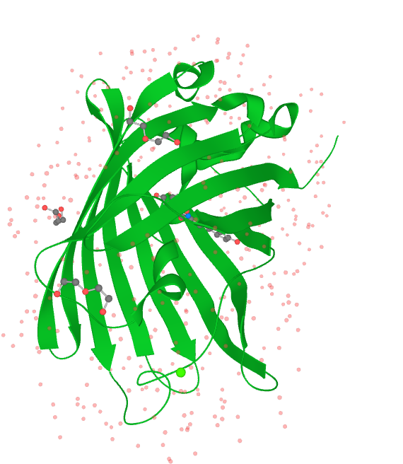
Figure 1: A computer rendering of the structure of the mEGFP[13, 29]. The $\beta$-strands around the exterior form the $\beta$-barrel structure. An $\alpha$-helix contains the chromophore that runs through the centre.

There are numerous techniques to model the non-Markovian dynamics induced by the environment in the system. Often, these techniques require the deployment of approximations to yield closed-form solutions or have convenient computation times. Furthermore, for systems that are coupled only weakly to their environment, we may deploy perturbative approaches such as the second-order perturbation time-convolutionless master equation [30]. Another approximation commonly utilized within the field of quantum optics is the rotating wave approximation, which neglects terms in the interaction Hamiltonian that have rapidly rotating phase contributions[31]. Such an approximation is helpful in low-temperature systems where the environmental frequencies are approximately equal to the transition frequency of a two-level system that is the system of interest. This is convenient as it allows for the restriction of the Hilbert space into a subspace of a fixed excitation number [32].

However, there exist a large number of systems wherein the approximations listed above are not valid. For example, for systems at moderate temperatures as well as intermediate coupling strengths, which are characterized by timescales overlapping between system and environment, these previous approaches become less useful and lead to anomalous results[25]. To fully understand how decoherence occurs in these physical systems, a better scheme is required. Such an approach that is numerically exact is the hierarchical equations of motion (HEOM) [33, 34]. This is a non-perturbative, non-Markovian and not limited to high-temperature equation of motion for quantum systems coupled to structured environments. This approach collects dominant degrees of freedom in the environment by generating a hierarchy of equations from repeated time derivatives of the path integral.

In this article, we will attempt to unveil the origins of the anomalous timescales in the dynamics of the GFPs by extending on the approaches of Gilmore and McKenzie [35, 8, 36] to study the effects of dielectric relaxation on the coherence dynamics of a model system for the GFP chromophore, this allows for the encapsulation of the non-Markovian dynamics present. In Section II, we cover the derivation of the spin-boson Hamiltonian model for understanding the dynamical decoherence of chromophores; this is done by assuming the chromophore can appropriately be modelled by a two-level quantum dipole. Section III covers the solving scheme utilized in the rest of the article, the hierarchical equations of motion, and how we can generate these from a generic bath correlation function. In Section IV, we utilize the Fluctuation and Dissipation Theorem of Kubo  [37] to derive a spectral density for our chromophore system and, by extension, its bath correlation function, which characterizes the environment’s impact on the system. In Section V, we derive a model for the two-chromophore coherent energy transfer, such a Hamiltonian is also formulated as a spin-boson model by utilizing a conserved quantity in the system. In Section VI, we show the results of the simulations of our models for a GFP system and explore the decoherence in an independent chromophore and a coherently coupled two-chromophore system and compare these results to the Markovian results generated by the Bloch-Redfield equations. In Section VII, we validate our non-Markovian negative entropy production result by studying the von-Neumann entropy and its evolution under the time-dependent Gorini–Kossakowski–Sudarshan–Lindblad (GKSL) equation [38].

II Spin boson model of a chromophore

We begin our study on the decoherence of chromophores embedded in biological complexes by dielectric relaxation through modelling the chromophore as a quantum point dipole in a quantized electromagnetic field. Two types of dipoles are present within such a system. Firstly, we have permanent dipoles generated by the anisotropy of the highest occupied molecular orbital (HOMO) and the lowest unoccupied molecular orbital (LUMO) of the chromophore [39]. Secondly, we have the purely quantum transition dipoles responsible for dissipation and excitation transfer via coupling to the electromagnetic field. The transition dipole is generated by the overlap of the HOMO and LUMO states on the electric dipole. Such a quantum dipole within an electromagnetic field will have an interaction energy given by $H_{I}=-\vec{d}(t)\cdot\vec{E}(t)$ where $\vec{E}$ is the time-dependent electric field and $\vec{d}$ is the electric dipole associated with the spin system. Performing a canonical quantization for this interaction yields

$$H_{I}=\begin{pmatrix}\vec{d}_{11}&\vec{d}_{12}\\ \vec{d}_{12}^{*}&\vec{d}_{22}\end{pmatrix}\cdot\vec{E}.$$ (1)

We have expressed the dipole operator in the energy eigenbasis of the system such that $\vec{d}_{ij}=\bra{i}\vec{d}\ket{j}$, where $\ket{1}$ and $\ket{2}$ are the HOMO and LUMO states of the system. We can rewrite the above in explicit operator form as

$$H_{I}=(\vec{d}_{11}\sigma_{+}\sigma_{-}+\vec{d}_{22}\sigma_{-}\sigma_{+}+\vec{d}_{12}\sigma_{+}+\vec{d}_{12}^{*}\sigma_{-})\cdot\vec{E},$$ (2)

where $\vec{E}=\sum_{\lambda}g_{\lambda}(a_{\lambda}+a^{\dagger}_{\lambda})\vec{e}_{\lambda}$ is the quantised field operator. $g_{\lambda}$ is the coupling strength of the $\lambda$ mode in the electromagnetic field to the point dipole, $a^{({\dagger})}_{\lambda}$ is the annihilation (creation) operator for the $\lambda$ mode and $\vec{e}_{\lambda}$ is the associated unit vector for the $\lambda$ mode accounting for the polarisation of the electromagnetic field. Introducing the parameters $\Delta\vec{d}=\frac{\vec{d}_{11}-\vec{d}_{22}}{2}$, $\vec{d}_{+}=\frac{\vec{d}_{11}+\vec{d}_{22}}{2}$, $\vec{d}_{T}^{R}+i\vec{d}_{T}^{I}=\vec{d}_{12}$, we can recast the above equation in terms of Pauli operators for the two-level dipole as

$$H_{I}=(\Delta\vec{d}\sigma_{z}+\vec{d}_{+}\mathds{1}+\vec{d}_{T}^{R}\sigma_{x}-\vec{d}_{T}^{I}\sigma_{y})\cdot\vec{E}.$$ (3)

The identity term will not directly influence the system’s dynamics. However, it will cause fluctuations within the environment acting as an effective driving force and is expected to have negligible impact on the coherence dynamics [22]. We also note that the terms associated with energetic transitions in the dipole, and thus radiative decay of the system, are those associated with $\sigma_{x,y}$ operators. The radiative decay of optically excited biomolecules occurs on time scales of ns. In contrast, decoherence occurs on timescales of less than a few ps and, as such, can be neglected. After these simplifications, the reduced Hamiltonian is

$$H_{I}=\sigma_{z}\Delta\vec{d}\cdot\vec{E}.$$ (4)

Furthermore, the free Hamiltonian operators of the system and electromagnetic field are given by

$$H_{S} =\frac{\omega_{0}}{2}\sigma_{z},$$ (5)

$$H_{E} =\sum_{\lambda}\omega_{\lambda}a^{\dagger}_{\lambda}a_{\lambda}.$$ (6)

where $\omega_{0}$ is the transition energy of the chromophore and $\omega_{\lambda}$ is the energy associated with the $\lambda$ mode of the electromagnetic field.

III Coupled chromophores spin-boson model

For two spatially localized chromophores, their transition dipoles will interact with each other via dipole-dipole interaction, which enables the F ”orster resonant energy transfer. Such transfer allows for direct, non-radiative exchange of excitations between the chromophores. The Hamiltonian associated with a coupled chromophore system is given by

$$H= \frac{1}{2}\omega_{1}\sigma_{z}^{1}+\frac{1}{2}\omega_{2}\sigma_{z}^{2}+\Delta d_{1}\sigma_{z}^{1}E_{1}+\Delta d_{2}\sigma_{z}^{2}E_{2}$$

$$+\frac{\kappa d_{1}d_{2}}{n^{2}R^{3}\epsilon_{0}}(\sigma_{+}^{1}\sigma_{-}^{2}+\sigma_{-}^{1}\sigma_{+}^{2})+H_{B1}+H_{B2}.$$ (7)

Here, $\Delta d_{i}$ is the difference between the ground and excited state electric dipole for the $i$th chromophore. $\omega_{i}$ is the transition energy from the ground state to the first excited state of the ith chromophore. $\kappa$ is the orientation factor determined by the relative angle between the two chromophores, $d_{i}$ is the $i$th chromophore’s transition dipole moment $E_{i}$ is the electric field operator that couples the $i$th chromophore to its local electromagnetic field bath and $H_{Bi}$ is the $i$th chromophore’s local bath’s free Hamiltonian given by

$$H_{Bi}=\sum_{\lambda}\omega_{\lambda i}a^{\dagger}_{\lambda i}a_{\lambda i}.$$ (8)

$R$ is the radial distance between the two chromophores, and $n$ is the refractive index of the solvent.

As presented above, the coupled chromophore Hamiltonian is equivalent to two single chromophore Hamiltonians with a coherent coupling term between the chromophores. This interaction is mediated by the dipole-dipole interactions of the two chromophores. Therefore, its magnitude is relatively weak and short-ranged due to the $1/R^{3}$ dependence in the coupling strength. By noting the time invariance of the chromophore’s excitation number operator, we have $N=\sigma_{z}^{1}+\sigma_{z}^{2}+2$, as $[H,N]=0$. This property allows us to limit our analysis to the two-dimensional subspace of the two chromophores system spanned by the degrees of freedom associated with $\{\ket{e}_{1}\otimes\ket{g}_{2},\ket{g}_{1}\otimes\ket{e}_{2}\}$, with $\ket{e,g}_{i}$ representing the excited and ground states of the $i$th chromophore.

Consequently, we can map the Hamiltonian for this single-excitation subspace to a reduced Hamiltonian given by

$$H=\frac{1}{2}\omega\sigma_{z}+\Lambda\sigma_{x}+\sigma_{z}V+B_{1}+B_{2},$$ (9)

with the $\omega=\omega_{1}-\omega_{2}$ difference between the two chromophore transition energies and where

$$V=\Delta d_{1}E_{1}-\Delta d_{2}E_{2},$$ (10)

and

$$\Lambda=\frac{\kappa d_{1}d_{2}}{n^{2}R^{3}\epsilon_{0}}.$$ (11)

The problem is now equivalent to a single spin-boson model with a tunnelling term ($\propto\Lambda$) between the two states. We note that the levels of this two-level system correspond to the singly excited states of the two chromophores such that $\ket{1}=\ket{e}_{1}\otimes\ket{g}_{2}$ and $\ket{0}=\ket{g}_{1}\otimes\ket{e}_{2}$. If we assume the two environments are uncorrelated due to a suitable spatial separation, the spectral density associated with the system is simply the sum over the individual chromophore spectral densities

$$J(\omega)=J_{1}(\omega)+J_{2}(\omega).$$ (12)

As expected, this yields a spin-boson model with an additional tunnelling term governing the energy transfer between chromophores.

The formalism presented above provides the spin-boson model for decoherence or dephasing. Such models have been studied extensively, but previous studies were within a limited regime characterized by weak coupling or Markovian approximations imposed upon the dynamics. In our approach, the only other parameter required to characterize the system fully is the spectral density $J(\omega)$.

IV Spectral Density

In order to study the dynamics of the system, we need to identify a spectral density that models the structure associated with the local environment. Here, we use the Fluctuation and Dissipation Theorem and follow the Caldeira-Leggett approach[21] to the zero-temperature fluctuations of a bosonic environment to the spectral density. The reaction field $E$ has the zero temperature correlation function

$$C(t)=\langle E(t)E(0)\rangle=\bra{0}E(t)E(0)\ket{0},$$ (13)

where the ground state of the free electric field is denoted by $\ket{0}$. One can then define the real part of the Fourier transformed correlation function - by utilizing the Sokhotski-Plemelj theorem - as

$$S_{R}(\omega)=\Re{\tilde{C}(\omega)}=\pi\sum_{\lambda}\delta(\omega_{0}-\omega_{\lambda})\lvert\bra{0}E\ket{\lambda}\rvert^{2}.$$ (14)

By returning to the definition of the electric field operator

$$E=\sum_{\lambda}g_{\lambda}(a^{\dagger}_{\lambda}+a_{\lambda}),$$ (15)

it is now clear that the only contributions from $\lvert\bra{0}E\ket{\lambda}\rvert^{2}$ are singly excited states of the electromagnetic field. This then yields

$$S_{R}(\omega)=\pi\sum_{\lambda}g_{\lambda}^{2}\delta(\omega-\omega_{\lambda}),$$ (16)

which is simply a multiple of the spectral density of the system

$$J(\omega)=\frac{\Delta d^{2}}{\pi}S_{R}(\omega).$$ (17)

In order to calculate the zero-temperature correlation function, we utilize an Onsager model[40]. Then the electromagnetic field operator and the dipole operator $d$ are related by the linear response function $\chi(t)$ such that the Fourier transform is given by $\tilde{E}(\omega)=d(\omega)\chi(\omega)$, where $\chi(\omega)$ is the frequency-dependent electric susceptibility. By utilizing the quantum fluctuation-dissipation theorem, we can show that the imaginary part of the Fourier transformed susceptibility $\chi(\omega)$ is $\tilde{S}(\omega)=2\Im{\chi(\omega)}$. In order to derive the electric susceptibility of the local environment around the dipole, $\chi=E/d=-\nabla\phi/d$, we employ Poisson’s equation $\nabla^{2}\phi=-\rho/\epsilon$ and impose the condition that $\phi$ and $\epsilon\nabla\phi$ are continuous in the domain considered. Here, $\phi$ is the electric potential, $\rho$ is the local charge density, and $\epsilon$ is the local dielectric constant. For the system architecture shown in Fig. 2(a) modelling a chromophore embedded within a protein structure of radial extent $r$ with dielectric $\epsilon_{p}$ within a solvent environment of dielectric $\epsilon_{s}$ the frequency-dependent electrical permittivity is then given by

$$\chi(\omega)=\frac{1}{4\pi\epsilon_{0}r_{2}^{3}}\frac{2(\epsilon_{s}-\epsilon_{p})}{2\epsilon_{s}+\epsilon_{p}}.$$ (18)

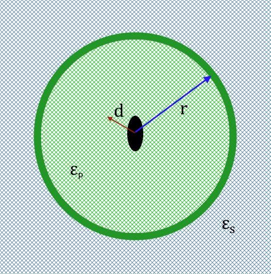
(a)

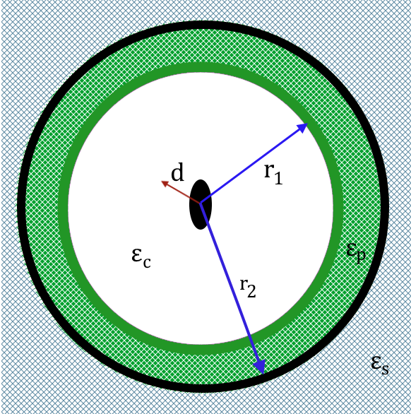
(b)

Figure 2: System architectures for models of chromophores given by dipole $d$ embedded within (a) protein complex with dielectric given by $\epsilon_{p}$ with radius $r$ inside of solvent medium with dielectric $\epsilon_{s}$. (b) a cavity of radius $r_{1}$ with dielectric $\epsilon_{c}$ in a protein complex of radius of radius $r_{2}$ and dielectric $\epsilon_{p}$ inside of solvent medium with dielectric $\epsilon_{s}$.

We may also increase the complexity of our system architecture by introducing a cavity of radius $r_{1}$ as shown in Fig. 2(b) leading to a dielectric of the form

$$\chi(\omega)=\frac{1}{4\pi\epsilon_{0}r_{1}^{3}}\frac{(\epsilon_{p}+2)(\epsilon_{s}-\epsilon_{p})r_{1}^{3}+(\epsilon_{p}-1)(2\epsilon_{s}+\epsilon_{p})r_{2}^{3}}{2(\epsilon_{p}-1)(\epsilon_{s}-\epsilon_{p})r_{1}^{3}+(2\epsilon_{p}+1)(2\epsilon_{s}+\epsilon_{p})r_{2}^{3}}.$$ (19)

In principle, all the dielectrics are frequency dependent. However, due to the small extent of the protein, variations in the solvent environment will be the most critical to the dynamics. For the standard solvent - water - we can characterize the low-frequency dielectric spectral region using a Debye model, with a frequency-dependent dielectric permittivity of the form

$$\epsilon(\omega)=\epsilon_{\infty}+\frac{\epsilon_{s}-\epsilon_{\infty}}{1+i\omega\tau_{D}}.$$ (20)

$\epsilon_{\infty}$ and $\epsilon_{s}$ are the high and low-frequency limit dielectrics for the solvent, respectively. For both system architectures considered in Fig. 1, this results in Ohmic spectral density with a Lorentz-Drude cutoff of the form,

$$J(\omega)=\frac{2\omega\lambda\gamma}{\pi(\omega^{2}+\gamma^{2})}.$$ (21)

$\lambda$ is the coupling strength and $\gamma$ the cut-off frequency.

From the Fluctuation and Dissipation theorem, we can relate the zero-temperature response to the finite temperature response through the correlation function

$$C(t)=\int^{\infty}_{0}d\omega\,J(\omega)\left[\text{coth}(\omega/2T)\,\text{cos}(\omega\tau)-i\,\text{sin}(\omega\tau)\right].$$ (22)

In order to determine the correlation function for this spectral density, we need to perform the Matsubara decomposition of the coth term such that

$$\text{coth}\left(\frac{\omega}{2T}\right)=2T\left(\frac{1}{\omega}+\sum_{k=1}^{\infty}\frac{2\omega}{\omega^{2}+(2\pi kT)^{2}}\right).$$ (23)

This allows for a term-by-term integration of the integral appearing in the correlation function, which yields a natural decomposition of the correlation function

$$C(t)=\sum^{\infty}_{k=0}c_{k}e^{-\nu_{k}t},$$ (24)

with the frequencies given by

$$\nu_{k}=\begin{cases}\gamma&k=0\\ {2\pi kT}&k\geq 1\\ \end{cases},$$ (25)

and the amplitudes by

$$c_{k}=\begin{cases}\lambda\gamma(\cot(\gamma/2T)-i)&k=0\\ 4\lambda\gamma\nu_{k}T/(\nu_{k}^{2}-\gamma^{2})&k\geq 1\\ \end{cases}.$$ (26)

However, as described above, this single Debye timescale only describes the dielectric’s permittivity at low frequencies. To spectral responses in the optical regime - relevant to the bio-molecular complexes - we need to introduce a secondary timescale. In this regime, the dielectric for water can be well described by a double Debye model [41] given by

$$\epsilon(\omega)=\epsilon_{\infty}+\frac{\epsilon_{s}-\epsilon_{1}}{1+i\omega\tau_{D}}+\frac{\epsilon_{1}-\epsilon_{\infty}}{1+i\omega\tau_{1}}.$$ (27)

Such a dielectric generates spectral densities of the form

$$J(\omega)=\lambda\frac{a\omega+b\omega^{3}}{c+d\omega^{2}+f\omega^{4}},$$ (28)

with the explicit parametrization of these variables given in Appendix. A. Due to the even nature of the integrand, we extend the integral between $[-\infty,\infty]$ such that

$$C(t)=\frac{1}{2}\int^{\infty}_{-\infty}d\omega\,J(\omega)\left[\text{coth}(\omega/2T)\,\text{cos}(\omega\tau)-i\,\text{sin}(\omega\tau)\right].$$ (29)

Considering now the contour integral in the upper half plane and using the residue theorem, we need only calculate the poles associated with the spectral density factor and the $\coth$ term. For the temperature-dependant $\coth$ term, the poles are simply at the Matsubara frequencies, $\omega_{k}=\pm 2\pi ikT$ . Similarly, the poles in the spectral density occur at

$$\omega=\pm\sqrt{\frac{-d\pm\sqrt{d^{2}-4cf}}{2f}}.$$ (30)

Altogether, the bath correlation function can be written as

$$C(t)=\frac{\lambda\pi}{2\kappa}\sum_{j=+,-}-j(a-b\alpha_{j}^{2})e^{-\alpha_{j}t}\left[\text{cot}\left(\frac{\alpha_{j}}{2T}\right)-i\right]+\sum_{n=1}^{\infty}2\pi\lambda T\frac{e^{-\omega_{n}t}\omega_{n}(-a+b\omega_{n}^{2})}{c-d\omega_{n}^{2}+f\omega_{n}^{4}},$$ (31)

where $\kappa=\sqrt{d^{2}-4cf}$ and $\alpha_{\pm}^{2}=\dfrac{d\pm\kappa}{2f}$ are the poles associated with the spectral density. This can then be recast as the standard series representation of the correlation function

$$C(t)=\sum_{k=-1}^{\infty}c_{k}e^{-\nu_{k}t},$$ (32)

with the frequencies given by

$$\nu_{k}=\begin{cases}\alpha_{-}&k=-1\\ \alpha_{+}&k=0\\ {2\pi k}T&k\geq 1\\ \end{cases},$$ (33)

and the amplitudes by

$$c_{k}=\begin{cases}\frac{\lambda\pi}{2\kappa}(a-b\alpha_{-}^{2})\left[\text{cot}\left(\frac{\alpha_{-}}{2T}\right)-i\right]&k=-1\\ \frac{\lambda\pi}{2\kappa}(b\alpha_{+}^{2}-a)\left[\text{cot}\left(\frac{\alpha_{+}}{2T}\right)-i\right]&k=0\\ 2\pi\lambda T\frac{\nu_{k}(-a+b\nu_{k}^{2})}{c-d\nu_{k}^{2}+f\nu_{k}^{4}}&k\geq 1\\ \end{cases}.$$ (34)

This form of the correlation function allows us to directly compare the single versus the double Debye models and identify the relevant time scales in the problem. We also note that the thermal fluctuations in the environment produce additional timescales in the system’s dynamics, precisely at each of the Matsubara frequencies. Furthermore, the spectral density of the double Debye model has a super-Ohmic character for higher energies signalling that compared to the single Debye model, the system will interact stronger with electromagnetic modes located at higher frequencies in the electromagnetic spectrum.

To fully resolve the dynamics of these models introduced, we need a non-Markovian, non-perturbative approach. This is because we expect the environment to provide non-negligible information feedback to the system, allowing for coherence extensions and thus not limited to the weak coupling regime. In order to explore this noon-perturbative and non-Markovian regime, we adopt the approach of the hierarchical equations of motion (HEOM).

V Hierarchical Equations of Motion

The hierarchical equations of motion (HEOM) method utilizes a discretization of the environment to generate a numerically efficient approach to capturing the effects of the collective degrees of freedom of the environment. This is achieved by constructing coupled differential equations that form a hierarchy from repeated time-derivatives of the influence functional, derived initially by Vernon and Feynman [42]. Such an approach is non-perturbative and allows for the exploration of strongly coupled systems with a non-zero temperature environment[33]. A fundamental assumption in this approach is that the system couples linear to its environment and that the bath correlation functions can be conveniently decomposed in a Fourier series. For a generic environment spectral density, this decomposition will be non-trivial; as such, we may adopt a numerical approach by fitting with spectral densities that do have convenient decompositions.

Another limitation of the HEOM method is the absence of a general approach in deciding how to truncate the hierarchy - which is infinite for a bosonic environment - and the Fourier decomposition of the correlation functions. The truncation is dependent on the initial temperature of the environment as well as the complexity of the spectral density associated with it.

In our work, we are specifically interested in bosonic reservoirs and their influence on the two-level systems. This is because we are modelling the electromagnetic field - a bosonic reservoir - and its interactions with the quantum dipole - a two-level system - of the chromophore. The Hamiltonian for a system interacting with a bosonic environment utilizing the second quantization is simply

$$H=H_{S}+\sum_{\lambda}\omega_{\lambda}a^{\dagger}_{\lambda}a_{\lambda}+Q\sum_{\lambda}g_{\lambda}(a_{\lambda}+a^{\dagger}_{\lambda}).$$ (35)

where $H_{S}$ is the free system Hamiltonian, and $Q$ is the coupling operator in the system’s degrees of freedom. For convenience, we introduce the bath operator

$$E=\sum_{\lambda}g_{\lambda}(a_{\lambda}+a_{\lambda}^{\dagger}).$$ (36)

By utilizing the Feynman-Vernon influence functional approach to path integrals, we can define the time evolution of the reduced density matrix as

$$\tilde{\rho}_{S}(t)=\mathcal{T}\text{exp}\left\{-\int^{t}_{0}dt_{2}\int^{t_{2}}_{0}dt_{1}Q^{\times}(t_{2})[C_{R}(t_{2}-t_{1})Q^{\times}(t_{1})+iC_{I}(t_{2}-t_{1})Q^{o}(t_{1})]\right\}\rho_{S}(0)$$ (37)

The tilde on the density operator signals that we are working in the interaction picture at time $t$, such that operators transform under the rule $A\rightarrow e^{i(H_{S}+H_{E})t}Ae^{-i(H_{S}+H_{E})t}$, where $H_{B}=\sum_{\lambda}\omega_{\lambda}a^{\dagger}_{\lambda}a_{\lambda}$ is the free environment Hamiltonian. We also assume that the initial state of the entire system is unentangled: $\rho(0)=\rho_{S}(0)\otimes\rho_{B}$ where $\rho_{B}$ is the thermalized Gibbs state given by

$$\rho_{B}=\frac{e^{-\beta H_{B}}}{Z},$$ (38)

where the inverse temperature of the reservoir $\beta=1/T$ and $Z=\text{tr}\{e^{-\beta H_{B}}\}$. Here, we have also introduced the notation for the commutator and the anticommutator

$$Q^{\times}=[Q,\cdot]\text{, and }Q^{0}=\{Q,\cdot\}.$$ (39)

Due to the harmonic nature of the environment, we can assume the environment acts as a Gaussian noise source, as described in the fluctuation-dissipation theorem. Under this assumption, the induced dynamics depend only on the second-order correlations of the environment defined by

$$C(\tau) =\langle E(t+\tau)E(t)\rangle$$ (40)

$$=\int^{\infty}_{0}d\omega J(\omega)\left[\text{coth}(\beta\omega/2)\text{cos}(\omega\tau)-i\text{sin}(\omega\tau)\right].$$

To facilitate the introduction of a hierarchical set of equations of motion, we decompose these correlation functions into real and imaginary parts

$$C(t)=C_{R}(t)+iC_{I}(t),$$ (41)

and corresponding Fourier components

$$C_{R}(t)=\sum^{N_{R}}_{k=1}c_{k}^{R}e^{-\gamma_{k}^{R}t},$$ (42)

$$C_{I}(t)=\sum^{N_{I}}_{k=1}c_{k}^{I}e^{-\gamma_{k}^{I}t},$$ (43)

where the coefficients $c_{k}^{R,I}$ and frequencies $\gamma^{R,I}_{k}$ can, in principle, be complex-valued. Applying consecutive time derivatives on the time evolution of the reduced density matrix described in Eq. 37, we generate an infinite set of coupled first-order equations of the form

$$\dot{\rho}^{n}(t) =\left(-iH^{\times}_{S}-\sum_{j=R,I}\sum_{k=1}^{N_{j}}n_{jk}\gamma^{j}_{k}\right)\rho^{n}(t)$$

$$-i\sum^{N_{R}}_{k=1}c_{k}^{R}n_{Rk}Q^{\times}\rho^{n^{-}_{Rk}}(t)+\sum^{N_{I}}_{k=1}c_{k}^{I}n_{Ik}Q^{o}\rho^{n^{-}_{Ik}}(t)$$

$$-i\sum_{j=R,I}\sum_{k=1}^{N_{j}}Q^{\times}\rho^{n^{+}_{jk}}(t),$$ (44)

where we have introduced the multi-index $n=(n_{Ri},n_{Ii}),n_{R,Ii}\in\{0,...,N_{c}\}$ where $N_{c}$ is the cutoff parameter defining the depth of the hierarchy to allow for convergence. The only physical density matrix is the $(0,...,0)$ indexed matrix and refers to the reduced density matrix. All other $\rho^{n}$ are auxiliary and encapsulate the collective environmental effects. The terms carrying an index $n^{\pm}_{jk}$ refer to auxiliary density operators with an index raised or lowered by one.

For the case of the interaction Hamiltonian given in Eq. 4, we have that $Q=\sigma_{z}$. In order to deploy the HEOM framework, we need only characterize the associated spectral density of the environment the biomolecule sits in.

VI Results

We now deploy the HEOM formalism to explore the dynamics of the single and dimeric chromophore systems. The model system we consider is that of the GFP. Such a system is of interest as it has been experimentally suggested that the decoherence timescale is anomalously long compared to other biomolecules, on the order of ps. Furthermore, the cylindrical shape of the $\beta$-barrel surrounding the small chromophore allows for compatibility with the structural architectures studied in Models 1, 2 and 3. The chromophore in GFP has a transition energy at $490$nm, giving it its distinct green coloration. Figure 3 shows the spectral densities of the three models we consider in our study using system parameters commonly available when classifying green fluorescent proteins, given in Table.1: model 1: a simple protein solvent environment described by a single Debye timescale as in Fig. 2(a); model 2: for a cavity protein solvent environment with a single Debye timescale as in Fig. 2(b); model 3: for a cavity protein solvent environment with a double Debye timescale as in Fig. 2(b). These parameters generate effective timescales for the spectral densities ($\gamma^{-1}$,$\alpha_{\pm}^{-1}$) of $0.63$ps for model 1, $0.62$ps for model 2 and $0.99$ and $0.24$ps for model 3 that has two effective timescales, due to the double Debye model. Clearly, for model 1, due to the chromophore being in direct contact with the protein, the coupling is significantly stronger compared to models 2 and 3, wherein the chromophore is embedded within a cavity of a significantly lower dielectric. Here, models 2 and 3 have the same system geometry, but different numbers of Debye timescales used to model the dielectric nature of the solvent; model 3 with two Debye timescales has lower coupling strength for small frequencies, compared to model 2, but for higher frequencies, this relationship is inverted, due to the super-Ohmic nature of the spectral density.

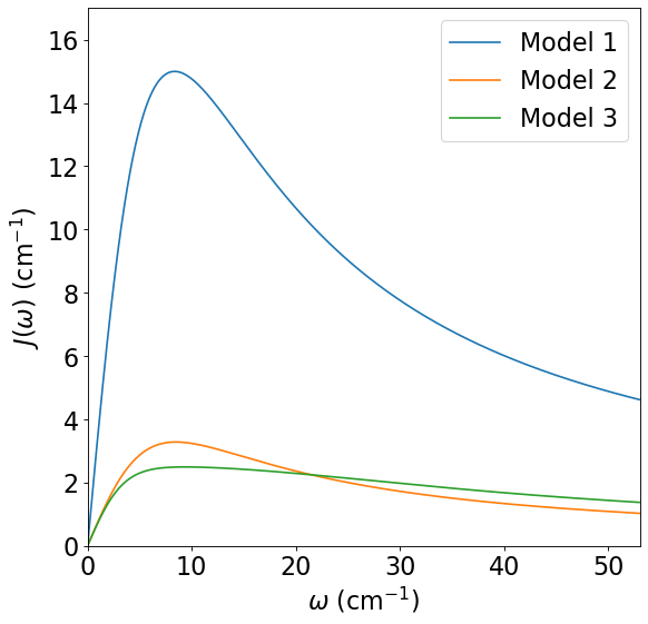
Figure 3: Spectral density associated with a GFP under different approximations of its structure. Model 1: a simple protein solvent environment described by a single Debye timescale as in Fig. 2(a). Model 2: for a cavity protein solvent environment with a single Debye timescale as in Fig. 2(b). Model 3: for a cavity protein solvent environment with a double Debye timescale as in Fig. 2(b).

To fully understand to what extent the non-Markovian effect influence the dynamics of the system considered, we also present a purely Markovian set of results and contrast them with the results produced by the HEOM method. For the Markovian approach, we adopt the Bloch-Redfield formalism, which is equivalent to a second-order perturbation master equation with an additional Markov approximation of the second kind and removal of energy Lamb shifts induced by the environment[43, 30] (see Appendix F).

A Single Chromophore System

We start by exploring the dynamical decoherence of the two-level chromophore system inside of a GFP environment. To unveil the coherence dynamics, we have chosen the initial condition to be the chromophore in a superposition state between the ground and excited state, with an initial density operator given by

$$\rho(0)=\frac{1}{2}\left(\ket{1}+\ket{0}\right)\left(\bra{1}+\bra{0}\right)\otimes\rho_{E}^{\beta}.$$ (45)

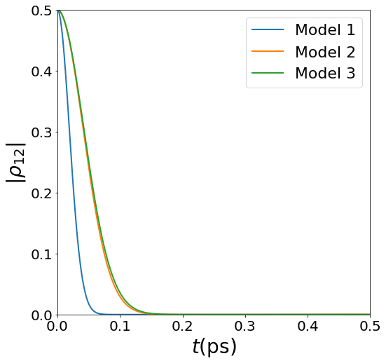
(a)

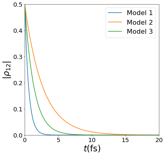
(b)

Figure 4: Dynamical decoherence of the two-level chromophore within GFPs using (a) the non-Markovian Hierarchical equations of motion (b) the Markovian Bloch-Redfield equations. The various models used are, Model 1: a simple protein solvent environment described by a single Debye timescale as in Fig. 2(a) Model 2: for a cavity protein solvent environment with a single Debye timescale as in Fig. 2(b) Model 3: for a cavity protein solvent environment with a double Debye timescale as in Fig. 2(b). The parameters were taken from the literature and are given in Table 1.

Figure 4 contrast the excitation dynamics of single chromophore structure under Markovian and non-Markovian approximations. Clearly, the exact dynamics of the system are sensitive to the model used for the surrounding environment: in model 1, the decay is considerably faster since the system is now in direct contact with the protein network leading to a stronger coupling as evidenced by the spectral densities shown in Figure 3. However, both model 2 and model 3 appear to have very similar dynamics in the HEOM regime. This is most likely because both system and interaction Hamiltonians are proportional to $\sigma_{z}$, which is not modulated in the interaction picture; hence, the low-frequency terms in the interaction play the dominant role in the dynamics of the system. As shown in Fig 3, that model 2 and model 3 have nearly identical spectral densities at low frequencies. We also note the sub-exponential decay of the coherence in the system in Fig. 4(a); at early times, the decay is less before saturating at later times. This time-dependent decay rate is a key characteristic of non-Markovian dynamics. Our results also predict that dielectric relaxation effects occur up to almost picosecond timeframes. This brings the theoretical modelling and experimental results data for the single GFP closer together[19, 20, 44] and demonstrates the efficacy of the HEOM approach to understanding the dynamical features of decoherence in these bio-molecular systems. Moreover, our results suggest that the solvent media dominates the decoherence rather than the specific protein dynamics. One would expect the specific frequency of oscillations is determined by the nature of the vibrational nature of the environment, but the solvent environment dominates the decoherence timescale.

The Bloch-Redfield results shown in Fig. 4(b), clearly demonstrate that the Markovian approximation predicts a much shorter decoherence times scale, hence the longer coherence times obtained in the HEOM formalism are associated with memory effects induced by information backflow from the environment to the system: under the non-Markovian system description the decoherence dynamics is dominated by ps time scales, whereas the Bloch-Redfield approach gives rise to time scales of the fs order. The failure of the Bloch-Redfield equations is apparent as we note that the most natural system timescale, associated with the transition frequency $\omega_{0}$, is significantly faster than the timescales associated with the environment as $\omega_{0}/\gamma\approx 2000$. This contradicts the necessary condition for the validity of the Markov approximation that underpins the Bloch-Redfield equations. Physically, we are demanding that the environment relaxes instantaneously and provides only a detriment to our system coherences. However, by allowing the environment to relax over an effective timescale commensurate with the system’s dynamics, we have an extension of the chromophore’s coherence lifetime. This can be traced back to the environment correlation functions in the Bloch-Redfield theory, the exponential decays are immediate, resulting in delta functions and thus no correlations, whereas in the entire system, the correlation function decays away at timescales of ps, considerably greater than the system timescale.

Further insight can be gained by writing down an analytical solution the Bloch-Redfield equations for $\rho_{12}$:

$$\rho_{12}=\rho_{12}(0)e^{-(2\Gamma+i\omega_{0})t}$$ (46)

with the rate constant

$$\Gamma=2\lambda T/\gamma,$$ (47)

for models 1 and 2. Clearly, then dynamics of the $\mathbf{l}_{1}$ norm coherence measure[45]

$$\mathbf{C}=2\absolutevalue{\rho_{12}}=2|\rho_{12}(0)|e^{-2\Gamma t}$$ (48)

is just a exponential decay. Since the decay rate $\Gamma$ is directly proportional to the coupling strength $\lambda$, we can explain the different dynamics displayed in Fig. 4(b): model 1 decays the fastest due to its higher coupling strength. However, this coupling strength dependence is not as stark in the full non-Markovian dynamics displayed in Fig. 4 as model 2 and 3 express very similar dynamics.

B Homo-dimer energy transfer

We now deal with a more exciting and challenging topic and consider the problem of coherent energy transfer between two-like GFPs, which can non-radiatively transfer excitations through dipolar interactions between the transition dipoles of both chromophores. We employ the Hamiltonian in Eq. 9, which for a homo-dimer system has site transition energy $\omega=0$ . We consider an initial state in which the first chromophore is in its ground state and the second is in its excited state. In the reduced single spin subspace, this can be expressed as $\rho=\ket{1}\bra{1}\otimes\rho_{B}^{\beta}$.

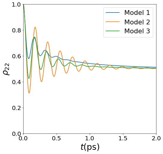
(a)

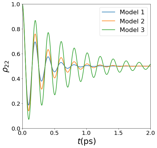
(b)

Figure 5: Excitation dynamics of two-coupled chromophores within GFPs using (a) the non-Markovian HEOM formalism (b) the Markovian Bloch-Redfield equations. The models used are shown in Figs. 2(a)-2(b). The parameters used are given in Table 1.

The homo-dimer GFP system excitation dynamics (see Fig. 5) is considerably richer than the one obtained in the monomeric case. Firstly, we note that in each of the models used, coherent energy transfer occurs due to the oscillations in the probability of the excitation being localized in the second chromophore $\rho_{22}$. These are in contrast with the non-oscillatory exponential decay associated with incoherent energy transfer. These oscillations occur much faster than the decoherence rate, allowing the excitation to be coherently transferred between the chromophores. It is worth recalling that the only difference between the models used is the associated spectral density, while the dipole-dipole interactions are identical. Hence, the modulations in the energy transfer rates - the periodicity of the oscillations - are purely induced by the interaction with the environment.

In the Bloch-Redfield regime, we note that the dynamics are qualitatively similar to the HEOM results. However, in the non-Markovian HEOM case, the oscillations are not about $\rho_{22}=\frac{1}{2}$ as in the Bloch-Redfield results; this is due to the Bloch-Redfield equation neglecting Lamb shifts in the systems. These Lamb shifts introduce an asymmetry in the transition energies between the two chromophores, suppressing the oscillations of the energy transfer, effectively making it more difficult to transfer energy. We also note that whilst the Model 3 system has a very long coherence lifetime in the Bloch-Redfield regime, in the HEOM results, we see that this timescale is shorter than that associated with model 2. This is due to the Bloch-Redfield solutions simply sampling the spectral density at the tunnelling rate $\Delta$, as we will show shortly, whereas, in the HEOM regime, nearby frequencies to the tunnelling rate will also play a key role.

We again consider the exact solutions for the homo-dimer Bloch-Redfield equations, with the population of the first chromophore given by

$$\rho_{11}=\frac{e^{-\gamma_{0}t}}{2\Gamma}\left(\gamma_{0}\sinh{\Gamma t}+\Gamma\cosh{\Gamma t}\right)+\frac{1}{2},$$ (49)

where the two effective rates are

$$\Gamma=\sqrt{\gamma_{0}^{2}-4\Lambda^{2}},$$ (50)

and

$$\gamma_{0}=8\pi J(2\Lambda)\coth{(\beta\Lambda)}.$$ (51)

As shown in Fig. 5(b), the $\Gamma$ rate is imaginary hence inducing coherent oscillations. However, the $\gamma_{0}$ rate is linearly dependent on the coupling strength $\lambda$ of our spectral density through $J(2\Lambda)$. This is not the case in the non-Markovian dynamics displayed in Fig. 5, please reformulate the following: where the model 1 description is coupled significantly stronger than in the other models. Our results show that the inter-chromophore coupling rate is of similar magnitude to the coupling strength with $\Lambda/\lambda\approx 3$ for models 2 and 3. In this regime, the system’s dynamics occur on timescales commensurate with the reorganization of the environment, which is not captured in the Markovian approximation, which asserts that the environment relaxes infinitely quickly. We can understand the difference between the effectiveness of the Bloch-Redfield solutions in the dimer case and the single GFP case. In the dimer case, the chromophores have the same energy, so the inter-site exchange requires no additional energy cost. The only relevant energy scale is associated with the inter-chromophore coupling. This is mediated by dipole-dipole interactions, a weak force, and is considerably smaller than the energy gap in the single chromophore system with $\frac{\omega_{0}}{\Lambda}\approx 300$. As such, the timescales in the single chromophore system are much faster, pushing the dynamics into a more non-Markovian regime, necessitating the HEOM approach. Considering a more physical situation in which (due to local asymmetries) there is a non-zero difference between the transition energies of the two chromophore $\omega=\omega_{1}-\omega_{2}\neq 0$, we find that the Bloch-Redfield equations are much less effective. The results presented in Fig. 6 show that even for a minimal asymmetry ($\omega=\omega_{1}-\omega_{2}=0.01\omega_{1}$) that the Bloch-Redfield theory is inadequate at capturing the system dynamics. This also suggests it would become impractical in the case of hetero-dimer systems, where the energy differences are considerably larger. Furthermore, we note that, in contrast, the HEOM results are robust to this type of perturbation.

Figure 6: The dynamics of the population dynamics of a chromophore in a Homo-Dimer of GFP, comparing the predictions of the Bloch-Redfield theory to the HEOM approach for a small asymmetry in the transition energies of the two chromophores: $\omega=\omega_{1}-\omega_{2}=0.01\omega_{1}$

To sum up, we note that for both the single chromophore and the homo-dimer systems, the Bloch-Redfield equations are insufficient at capturing the full dynamics as relevant rates in the system are directly proportional to the coupling strength $\lambda$. Another unexpected aspect of the dynamics of these models is the transient lowering of the von-Neumann entropy, as shown in Fig. 7, often associated with memory effects present in the system. Additionally, there is a direct correlation between the oscillations due to coherent energy transfer and the reduction of the von-Neumann entropy. We argue that precisely this interplay allows for an extension of the decoherence of the system compared to the single system, which we explore next.

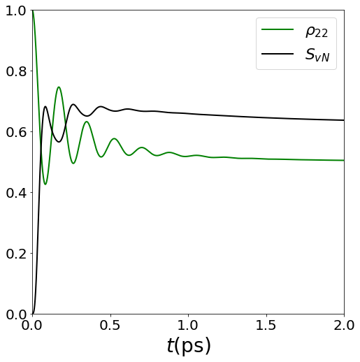
Figure 7: The population and entropy dynamics of a homo-dimer GFP in model 3: for a cavity protein solvent environment with a double Debye timescale.

VII Negative Entropy Production

In order to fully explore the implications of the complex dynamics described above, we focus now on the evolution of the system’s entropy. To this end we consider the von-Neumann entropy of a density matrix $\rho$ given by

$$S_{vN}=-\Tr{\rho\ln{\rho}}.$$ (52)

The entropy production can be found taking the time derivative

$$S_{vN}=-\Tr{\dot{\rho}\ln{\rho}}.$$ (53)

Using the HEOM-Gorini–Kossakowski–Sudarshan–Lindblad (GSKL) formalism mapping presented in Appendix D, we can rewrite the entropy production as

$$\dot{S}_{vN} =-\Tr{\ln{\rho}\sum_{\alpha,\beta}\Gamma_{\alpha\beta}\left(\sigma_{\alpha}\rho\sigma_{\beta}^{\dagger}-\frac{1}{2}\{\sigma_{\beta}^{\dagger}\sigma_{\alpha},\rho\}\right)}$$

$$=-\sum_{\alpha,\beta}\Gamma_{\alpha\beta}\Tr{\ln{\rho}\left(\sigma_{\alpha}\rho\sigma_{\beta}^{\dagger}-\rho\sigma_{\beta}^{\dagger}\sigma_{\alpha}\right)}.$$

Assuming that the cross terms in the previous equation can be neglected, the double sum reduces to a single sum. Then taking the operators $\{\sigma_{\alpha}\}$ to be the set of generalized Pauli operators (Hermitian and involutions, $\sigma_{\alpha}^{2}=\mathbf{1}$), we obtain

$$\dot{S}_{vN} =-\sum_{\alpha}\Gamma_{\alpha}\Tr{\ln{\rho}\left(\sigma_{\alpha}\rho\sigma_{\alpha}-\rho\right)}$$

$$=\sum_{\alpha}\Gamma_{\alpha}\left(\Tr{\rho\ln{\rho}}-\Tr{\tilde{\rho}_{\alpha}\ln{\rho}}\right)$$

$$=\sum_{\alpha}\Gamma_{\alpha}S(\tilde{\rho}_{\alpha}||\rho).$$ (54)

Here $\tilde{\rho}_{\alpha}=\sigma_{\alpha}\rho\sigma_{\alpha}$ is the basis transformation of the system state to that associated with eigenstates of the Lindblad operator $\sigma_{\alpha}$ and $S(\tilde{\rho}_{\alpha}||\rho)$ is the relative entropy of the density matrix coordinate transformed to the basis of $\sigma_{\alpha}$ with the untransformed density matrix.

Consequently, we expect the relative entropy to be non-negative valued and zero when $\rho_{\alpha}=\rho$. Therefore, negative entropy production requires that both rates $\Gamma_{\alpha}$, take negative values, which implies non-Markovian dynamics.

VIII Conclusion

To conclude, we have developed a framework to describe the decoherence of bio-molecules inside GFPs using a reduced spin-boson model. Our approach only includes decoherence induced by dielectric relaxation and predicts timescales of similar magnitude to those measured experimentally[19, 20, 44]. Our approach employs a reservoir spectral density derived directly from the fluctuation-dissipation theorem applied to the local electromagnetic field surrounding the chromophore. It fully captures the influence of dielectric properties of the environment on the chromophore dynamic. We demonstrated that different environmental configurations strongly affect the dynamical decoherence. Furthermore, we have shown the non-Markovian bi-directional flow of information between the system and dielectric environment plays an essential role in the system dynamics. We have also shown that certain configurations (single chromophore or the slightly asymmetric homo-dimer system) can lead to long decoherence timescales. Our exploration of the von-Neumann entropy evolution strongly supports the argument that the transient fluctuations in the entropy of the reduced system and the associated negative entropy production are also induced by non-Markovian effects. The formalism developed here can also find applications to investigating other complex bio-molecular systems undergoing coherent energy transfer, including hetero-dimers, trimers, tetramers and light-harvesting complexes.

Appendix A Parameters for GFP system

The parameters utilized throughout this paper are provided below in Table. 1.

Parameter	Value (units)
GFP transition wavelength	$490$nm [13]
$\Delta\mu$	10 D [7]
$\mu_{T}$	7.1 D[46]
$\kappa$	0.35[47]
$r_{2}$	$13.35$Å[48]
$r_{1}$	$5$Å[48]
$R$	$27.5$Å[49]
$n$	$1.72$[50]
$T$	$293$K
$\epsilon_{P}$	$4$[51]
Single Debye	[35]
$\tau_{D}$	$8.2$ps
$\epsilon_{\infty}$	$4.21$
$\epsilon_{S}$	$78.3$
Double Debye	[41]
$\tau_{D}$	$8.3$ps
$\tau_{1}$	$0.36$ps
$\epsilon_{\infty}$	$4.48$
$\epsilon_{1}$	$6.6$
$\epsilon_{S}$	$78.6$

Table 1: Relevant parameters for GFP system.

Appendix B Parameters for the Double Debye System

Here we introduce the two Debye timescale decay  [52] model for the solvent media, used to model the density of states of the electromagnetic field in the high-frequency regime, relevant for transitions in the optical regime.

We start with the following frequency dependant dielectric[41]

$$\epsilon(\omega)=\epsilon_{\infty}+\frac{\epsilon_{s}-\epsilon_{1}}{1-i\omega\tau_{D}}+\frac{\epsilon_{1}-\epsilon_{\infty}}{1-i\omega\tau_{1}},$$ (55)

which leads to spectral densities of the form

$$J(\omega)=\lambda\frac{a\omega+b\omega^{3}}{c+d\omega^{2}+f\omega^{4}}.$$ (56)

Here the parameters defining the model are related to the electric permittivity in Equation 19

$$\lambda= \frac{\Delta\mu^{2}}{8\pi^{2}\epsilon_{0}r_{1}^{3}}$$

$$a= 27r_{1}^{3}r_{2}^{3}\epsilon_{p}^{2}(\epsilon_{1\infty}\tau_{1}+\epsilon_{s1}\tau_{D}),$$

$$b= 27r_{1}^{3}r_{2}^{3}\epsilon_{p}^{2}\tau_{1}\tau_{D}(\epsilon_{s1}\tau_{1}+\epsilon_{1\infty}\tau_{D}),$$

$$c= (2r_{1}^{3}(-1+\epsilon_{p})(\epsilon_{1\infty}+\epsilon_{\infty}-\epsilon_{p}+\epsilon_{s1})+r_{2}^{3}(1+2\epsilon_{p})(2\epsilon_{1\infty}+2\epsilon_{\infty}+\epsilon_{p}+2\epsilon_{s1}))^{2},$$

$$d= (-4r_{1}^{3}r_{2}^{3}(-1-\epsilon_{p}+2\epsilon_{p}^{2})(-2(\epsilon_{s1}\tau_{1}+\epsilon_{1\infty}\tau_{D})^{2}-2\epsilon_{\infty}^{2}(\tau_{1}^{2}+\tau_{D}^{2})+\epsilon_{\infty}\epsilon_{p}(\tau_{1}^{2}+\tau_{D}^{2})$$

$$+\epsilon_{p}^{2}(\tau_{1}^{2}+\tau_{D}^{2})-4\epsilon_{\infty}(\epsilon_{s1}\tau_{1}^{2}+\epsilon_{1\infty}\tau_{D}^{2})+\epsilon_{p}(\epsilon_{s1}\tau_{1}^{2}+\epsilon_{1\infty}\tau_{D}^{2}))+r_{2}^{6}(1+2\epsilon_{p})^{2}(4(\epsilon_{s1}\tau_{1}+\epsilon_{1\infty}\tau_{D})^{2}$$

$$+4\epsilon_{\infty}^{2}(\tau_{1}^{2}+\tau_{D}^{2})+4\epsilon_{\infty}\epsilon_{p}(\tau_{1}^{2}+\tau_{D}^{2})+\epsilon_{p}^{2}(\tau_{1}^{2}+\tau_{D}^{2})+8\epsilon_{\infty}(\epsilon_{s1}\tau_{1}^{2}+\epsilon_{1\infty}\tau_{D}^{2})$$

$$+4\epsilon_{p}(\epsilon_{s1}\tau_{1}^{2}+\epsilon_{1\infty}\tau_{D}^{2}))+4r_{1}^{6}(-1+\epsilon_{p})^{2}((\epsilon_{s1}\tau_{1}+\epsilon_{1\infty}\tau_{D})^{2}+\epsilon_{\infty}^{2}(\tau_{1}^{2}+\tau_{D}^{2})$$

$$+\epsilon_{p}^{2}(\tau_{1}^{2}+\tau_{D}^{2})-2\epsilon_{p}(\epsilon_{s1}\tau_{1}^{2}+\epsilon_{1\infty}\tau_{D}^{2})+2\epsilon_{\infty}(\epsilon_{s1}\tau_{1}^{2}+\epsilon_{1\infty}\tau_{D}^{2}-\epsilon_{p}(\tau_{1}^{2}+\tau_{D}^{2})))),$$

$$f= (2r_{1}^{3}(\epsilon_{\infty}-\epsilon_{p})(-1+\epsilon_{p})+r_{2}^{3}(2\epsilon_{\infty}+\epsilon_{p})(1+2\epsilon_{p}))^{2}\tau_{1}^{2}\tau_{D}^{2},$$

$$\epsilon_{1\infty} =\epsilon_{1}-\epsilon_{\infty},$$

$$\epsilon_{s1} =\epsilon_{s}-\epsilon_{1}.$$ (57)

Appendix C Multiple Timescales

It has recently been a point of contention as to whether or not water is best described by a two or three timescale Debye solvent up to THz frequencies. Naturally, we would expect that as we probe higher and higher energy scales we will excite dynamic modes of these systems that resolve over smaller and smaller timescales. For a solvent medium that can be described by $N$ timescales, the frequency dependent dielectric is given by

$$\epsilon_{s}(\omega)=\epsilon_{\infty}+\sum^{N}_{j=1}\frac{\epsilon_{j}-\epsilon_{j+1}}{1+i\omega\tau_{j}}$$ (58)

we have that the correlation function is of the form

$$C(t)=\int^{\infty}_{0}d\omega\frac{P(\omega)}{Q(\omega)}\left[\coth{\left(\omega/2T\right)}\cos{\left(\omega t\right)}-i\sin{\left(\omega t\right)}\right].$$ (59)

$P(\omega)$ is an odd polynomial of order $N$, and $Q(\omega)$ is an even polynomial of order $2N$. If we consider the $2N$ roots of $Q(\omega)=0$ are the set of values $S=\{\omega^{(n)}\}$. As we shall see we need only consider the $N$ roots that satisfy $\Im{\omega^{(n)}}>0$ that form the set $S_{+}=\{\omega^{(n)}_{+}\}$. By considering the contour integral in the upper half plane, and noting that the integrand of the correlation function is even we have from the Residue theorem that

$$C(t)=\pi i\left[\sum_{\omega^{(n)}_{+}\in S_{+}}\frac{P(\omega^{(n)}_{+})}{2\omega^{(n)}_{+}Q_{R}(\omega^{(n)}_{+})}e^{i\omega^{(n)}_{+}t}\left(\coth{\left(\beta\omega^{(n)}_{+}/2\right)}-i\right)+\sum_{n=1}^{\infty}e^{-\omega_{n}t}\frac{2P(i\omega_{n})}{\beta Q(i\omega_{n})}\right]$$ (60)

where

$$Q_{R}(\omega^{(n)}_{+})=\lim_{\omega\to\omega^{(n)}_{+}}Q(\omega)(\omega^{2}-(\omega^{(n)}_{+})^{2})^{-1}.$$ (61)

For a sanity check, we can consider the form of the exponential components from the environment - those of the form $e^{i\omega^{(n)}_{+}t}$. We can note that as we have $\Im{\omega^{(n)}}>0$ then we necessarily have $\Re{\omega^{(n)}}<0$ as one would expect, providing us with no exponentially growing terms and thus nonphysical fluctuations.

This provides a general scheme to reform the $N$ timescale dielectrics in to a form commensurate with the HEOM approach. However, due to the polynomial nature of the solutions getting exact solutions is only generally possible for $N<5$ timescales. However, one could adopt a numerical approach to finding these roots.

Appendix D Mapping HEOM to time-dependant GKSL

For the single two-level system interacting with the bosonic environment given by

$$H=H_{A}+H_{B}+H_{I}$$ (62)

where

$$H_{A} =\frac{1}{2}\omega_{0}\sigma_{z}$$

$$H_{B} =\sum_{\lambda}\omega_{\lambda}a^{\dagger}_{\lambda}a_{\lambda}$$

$$H_{I} =\sigma_{z}\sum_{\lambda}g_{\lambda}(a^{\dagger}_{\lambda}+a_{\lambda})$$ (63)

One can note that the populations of the two-level systems free energy eigenstates will be unchanged in any evolution. As such we can directly compare any time evolution of the reduced density matrix for the two-level system $\rho_{A}$ to a GKSL-like equation of the form

$$\dot{\rho}_{A}=-i[H_{A}(t),\rho_{A}]+\Gamma\left(\sigma_{z}\rho_{A}\sigma_{z}-\rho_{A}\right)$$ (64)

where the Lindblad rate is time dependant and of the form

$$\Gamma(t)=-\frac{1}{2}\frac{\Re{\dot{\rho}_{12}}}{\Re{\rho_{12}}}.$$ (65)

For the case of the coupled chromophores which has Hamiltonian given by

$$H_{A}=\Delta\sigma_{x}$$ (66)

we now can note that the generic time evolution of the reduced density matrix is given by

$$\dot{\rho}_{A}=\begin{pmatrix}\dot{\rho}_{11}&\dot{\rho}_{12}\\ \dot{\rho}_{21}&\dot{\rho}_{22}\end{pmatrix}.$$ (67)

We can right the generic time evolution in the form of a time dependant GKSL equation of the form

$$\dot{\rho}_{A}=\sum_{i=\{x,y,z\}}\Gamma_{i}(\sigma_{i}\rho_{A}\sigma_{i}-\rho_{A})$$ (68)

where the Lindblad rates

$$\Gamma_{z}=\frac{1}{4}\left(\frac{2\dot{\rho}_{11}}{2\rho_{11}-1}-\frac{\imaginary(\dot{\rho}_{12})}{\imaginary(\rho_{12})}-\frac{\real(\dot{\rho}_{12})}{\real(\rho_{12})}\right)$$ (69)

$$\Gamma_{x}=\frac{1}{4}\left(\frac{2\dot{\rho}_{11}}{1-2\rho_{11}}-\frac{\imaginary(\dot{\rho}_{12})}{\imaginary(\rho_{12})}+\frac{\real(\dot{\rho}_{12})}{\real(\rho_{12})}\right)$$ (70)

$$\Gamma_{y}=\frac{1}{4}\left(\frac{2\dot{\rho}_{11}}{1-2\rho_{11}}+\frac{\imaginary(\dot{\rho}_{12})}{\imaginary(\rho_{12})}-\frac{\real(\dot{\rho}_{12})}{\real(\rho_{12})}\right)$$ (71)

or equivalently

$$\Gamma_{z}=\frac{1}{4}\frac{d}{dt}\left(\ln{\langle\sigma_{z}\rangle}+\ln{\langle\sigma_{y}\rangle}-\ln{\langle\sigma_{x}\rangle}\right)$$ (72)

$$\Gamma_{x}=\frac{1}{4}\frac{d}{dt}\left(-\ln{\langle\sigma_{z}\rangle}+\ln{\langle\sigma_{y}\rangle}+\ln{\langle\sigma_{x}\rangle}\right)$$ (73)

$$\Gamma_{y}=\frac{1}{4}\frac{d}{dt}\left(-\ln{\langle\sigma_{z}\rangle}-\ln{\langle\sigma_{y}\rangle}-\ln{\langle\sigma_{x}\rangle}\right)$$ (74)

Thus we can map the dynamics of HEOM directly onto GKSL-like equations. However, one should note that these Lindblad rates are trajectory dependant being functions of $\rho_{A}$.

Appendix E von-Neumman Entropy Rates

The von-Neumann entropy is defined as

$$S_{vN}=-\Tr{\rho\ln{\rho}}.$$ (75)

The generic form for a density operator is be given by

$$\rho=\sum^{N}_{i=1}p_{i}\ket{\phi_{i}}\bra{\phi_{i}}$$ (76)

where $p_{i}$ is the probability that the system is in the pure state given by $\phi_{i}$. The Mercator series for the logarithm of a matrix given by

$$\ln{\rho}=\sum_{n=1}^{\infty}(-1)^{n+1}\frac{(\rho-\mathbf{1})^{n}}{n}$$ (77)

is only definitely convergent for $||\mathbf{1}-\rho||<1$ where $||A||=\sqrt{\Tr{A^{\dagger}A}}$ denotes the Hilbert-Schmidt norm. For our density operator we have that

$$||\mathbf{1}-\rho||=\sqrt{\Tr{\sum^{N}_{i=1}(1-p_{i})\ket{\phi_{i}}\bra{\phi_{i}}\sum^{N}_{j=1}(1-p_{j})\ket{\phi_{j}}\bra{\phi_{j}}}}$$ (78)

$$=\sqrt{\sum^{N}_{i=1}(1-p_{i})^{2}}=\sqrt{\sum^{N}_{i=1}1-2p_{i}+p_{i}^{2}}$$ (79)

$$=\sqrt{N-2+\sum^{N}_{i=1}p_{i}^{2}}$$ (80)

as $0<\sum^{N}_{i=1}p_{i}^{2}\leq 1$ we have that

$$\sqrt{N-2}<||\mathbf{1}-\rho||\leq\sqrt{N-1}$$ (81)

and as such, to have definite convergence, we require $N=2$ denoting that the Mercator series is only strictly convergent for mixed states of two-level systems. If we restrict ourselves to the two-state Hilbert space we can now consider the entropy production by time differentiating the von-Neumann entropy, using the Mercator series.

$$S_{vN}=-\Tr{\rho\ln{\rho}}=-\Tr{\rho\sum_{n=1}^{\infty}(-1)^{n+1}\frac{(\rho-\mathbf{1})^{n}}{n}}.$$ (82)

differentiating with respect to time yields by the product rule

$$\dot{S}_{vN}=-\Tr{\dot{\rho}\ln{\rho}}-\Tr{\rho\frac{d}{dt}\ln{\rho}}.$$ (83)

The time-derivative of the logarithm term can be achieved by the Mercator projection

$$\frac{d}{dt}\ln{\rho}=\sum_{n=1}^{\infty}(-1)^{n+1}\frac{(\rho-\mathbf{1})^{n}}{n}$$ (84)

$$=\sum_{n=1}^{\infty}\frac{(-1)^{n+1}}{n}\sum_{i=0}^{n-1}(\rho-\mathbf{1})^{i}\dot{\rho}(\rho-\mathbf{1})^{n-i}.$$ (85)

Now if we consider the term

$$\Tr{\rho\frac{d}{dt}\ln{\rho}}$$ (86)

$$=\Tr{\rho\sum_{n=1}^{\infty}\frac{(-1)^{n+1}}{n}\sum_{i=0}^{n-1}(\rho-\mathbf{1})^{i}\dot{\rho}(\rho-\mathbf{1})^{n-i}}$$ (87)

$$=\Tr{\sum_{n=1}^{\infty}\frac{(-1)^{n+1}}{n}\sum_{i=0}^{n-1}\rho(\rho-\mathbf{1})^{i}\dot{\rho}(\rho-\mathbf{1})^{n-i}}$$ (88)

it is clear to see that $\rho$ commutes with $\rho-\mathbf{1}$ and then by the cyclic property of the trace we have

$$\Tr{\rho\frac{d}{dt}\ln{\rho}}\\ =\Tr{\sum_{n=1}^{\infty}(-1)^{n+1}(\rho-\mathbf{1})^{n-1}\rho\dot{\rho}}.$$ (89)

For the other term in the entropy production we can expand this with the Mercator series

$$\Tr{\dot{\rho}\ln{\rho}}=$$ (90)

$$\Tr{\sum_{n=1}^{\infty}(-1)^{n+1}\frac{(\rho-\mathbf{1})^{n}}{n}\dot{\rho}}.$$ (91)

We can then return to the definition of the Entropy production to show that

$$\dot{S}_{vN}=-\Tr{\sum_{n=1}^{\infty}(-1)^{n+1}\frac{(\rho-\mathbf{1})^{n}}{n}\dot{\rho}}$$ (92)

$$-\Tr{\sum_{n=1}^{\infty}(-1)^{n+1}(\rho-\mathbf{1})^{n-1}\rho\dot{\rho}}$$ (93)

$$=\sum_{n=1}^{\infty}(-1)^{n}\Tr{\frac{(\rho-\mathbf{1})^{n}}{n}\dot{\rho}+(\rho-\mathbf{1})^{n-1}\rho\dot{\rho}}$$ (94)

$$=\sum_{n=1}^{\infty}(-1)^{n}\Tr{(\rho-\mathbf{1})^{n-1}\left(\frac{(\rho-\mathbf{1})}{n}+\rho\right)\dot{\rho}}$$ (95)

$$=\sum_{n=1}^{\infty}\frac{(-1)^{n}}{n}\Tr{(\rho-\mathbf{1})^{n-1}\left((n+1)\rho-\mathbf{1}\right)\dot{\rho}}.$$ (96)

If we consider time evolution of $\rho$ to be determined by the time-dependent GKSL, due to the commuting nature of $\rho$ and $\rho-\mathbf{1}$ the free von-Neumann term naturally disappears. For convenience we denote

$$\hat{A}=\sum_{n=1}^{\infty}\frac{(-1)^{n}}{n}(\rho-\mathbf{1})^{n-1}\left((n+1)\rho-\mathbf{1}\right)$$ (97)

such that $[\rho,\hat{A}]=0$. Leaving

$$\dot{S}_{vN}=\Tr{\hat{A}\left(\sum_{\alpha,\beta}\gamma_{\alpha\beta}\left(\sigma_{\alpha}\rho\sigma_{\beta}^{\dagger}-\frac{1}{2}\{\sigma_{\beta}^{\dagger}\sigma_{\alpha},\rho\}\right)\right)}$$

$$= \Tr{\left(\sum_{\alpha,\beta}\gamma_{\alpha\beta}\left(\hat{A}\sigma_{\alpha}\rho\sigma_{\beta}^{\dagger}-\hat{A}\frac{1}{2}\{\sigma_{\beta}^{\dagger}\sigma_{\alpha},\rho\}\right)\right)}$$

$$= \sum_{\alpha,\beta}\gamma_{\alpha\beta}\Tr{\left(\hat{A}\sigma_{\alpha}\rho\sigma_{\beta}^{\dagger}-\hat{A}\frac{1}{2}\{\sigma_{\beta}^{\dagger}\sigma_{\alpha},\rho\}\right)}$$ (98)

$$= \sum_{\alpha,\beta}\gamma_{\alpha\beta}\Tr{\left(\hat{A}\sigma_{\alpha}\rho\sigma_{\beta}^{\dagger}-\hat{A}\frac{1}{2}\{\sigma_{\beta}^{\dagger}\sigma_{\alpha},\rho\}\right)}$$

$$= \sum_{\alpha,\beta}\gamma_{\alpha\beta}\left[\Tr{\hat{A}\sigma_{\alpha}\rho\sigma_{\beta}^{\dagger}}-\Tr{\hat{A}\frac{1}{2}\{\sigma_{\beta}^{\dagger}\sigma_{\alpha},\rho\}}\right]$$

$$= \sum_{\alpha,\beta}\gamma_{\alpha\beta}\left[\Tr{\hat{A}\sigma_{\alpha}\rho\sigma_{\beta}^{\dagger}}-\Tr{\hat{A}\rho\sigma_{\beta}^{\dagger}\sigma_{\alpha}}\right]$$

$$= \sum_{\alpha,\beta}\gamma_{\alpha\beta}\Tr{\hat{A}\left(\sigma_{\alpha}\rho\sigma_{\beta}^{\dagger}-\rho\sigma_{\beta}^{\dagger}\sigma_{\alpha}\right)}$$

For the case of dephasing on a two-level system such that the $\sigma=\sigma_{z}$

$$\dot{S}_{vN}^{z}=\gamma_{z}\Tr{\hat{A}\left(\sigma_{z}\rho\sigma_{z}-\rho\right)}.$$ (99)

If we now choose the basis for our density operator such that

$$\rho=\begin{pmatrix}\rho_{11}&\rho_{12}\\ \rho_{12}^{*}&1-\rho_{11}\end{pmatrix},$$ (100)

and

$$\sigma_{z}=\begin{pmatrix}1&0\\ 0&-1\end{pmatrix}.$$ (101)

Then we can find that

with $\nu=\sqrt{(\rho_{11}-\rho_{22})^{2}+4|\rho_{12}|^{2}}<1$ we can resolve the infinite sum to get

$$\dot{S}_{vN}^{z}=4\gamma_{z}|\rho_{12}|^{2}\ln\left(\frac{1+\nu}{1-\nu}\right)\nu^{-1}.$$ (102)

A similar analysis for $\sigma_{x}$ yields

$$\dot{S}_{vN}^{x}=\gamma_{x}(\rho_{11}-\rho_{22})^{2}\ln\left(\frac{1+\nu}{1-\nu}\right)\nu^{-1}.$$ (103)

We can note that the sign associated with these entropy production rates are solely determined by the sign of the GKSL time-dependant rates $\gamma$. This has previously been used as a marker for non-Markovianity, suggesting that the only way for a two-level system to have negative entropy production rates is to undergo non-Markovian dynamics.

Appendix F Bloch-Redfield Equations

By beginning with the von-Neumann equation, one can formally integrate the differential equation yielding

$$\rho(t)=\rho(0)-i\int^{t}_{0}dt_{1}[H,\rho(t_{1})]$$ (104)

by substituting this back into the von-Neumann equation we generate a new differential equation of the form

$$\dot{\rho}(t)=-i[H,\rho(0)-i\int^{t}_{0}dt_{1}[H,\rho(t_{1})]]$$ (105)

performing a partial trace over the environment and switching to the Dirac picture we get

$$\dot{\rho}_{S}=-\int^{t}_{0}dt_{1}\text{tr}_{E}\{[H_{I}(t),[H_{I}(t_{1}),\rho(t_{1})]]\}$$ (106)

at this stage we invoke the Born-Markov approximation such that we assume the environment is not perturbed by interacting with our system of interest -$\rho(t)=\rho_{S}(t)\otimes\rho_{E}$ (Born) - and that system’s evolution is only dependant on its current state $\rho(t_{1})\to\rho(t)$ (Markov) leading to the time local equation

$$\dot{\rho}_{S}=-\int^{t}_{0}dt_{1}\text{tr}_{E}\{[H_{I}(t),[H_{I}(t_{1}),\rho_{S}(t)\otimes\rho_{E}]]\}$$ (107)

The Born-Markov approximation is only valid if the system only lightly perturbs the environment such that the relaxation time of the environment is extremely fast compared to the dynamical processes of the system. If we are able to decompose the interaction Hamiltonian into bath and system operators as $H_{I}=\sum_{i}S_{i}\otimes B_{i}$ we can expand the above into

$$\dot{\rho}_{S}(t)= -\sum_{ij}\int^{t}_{0}dt_{1}\big{[}(S_{i}(t)S_{j}(t_{1})\rho_{S}(t)$$

$$-S_{j}(t_{1})\rho S_{i}(t))C_{ij}(t,t_{1})+(\rho_{S}(t)S_{j}(t_{1})S_{i}(t)$$

$$-S_{i}(t)\rho_{S}(t)S_{j}(t_{1}))C_{ji}(t_{1},t)\big{]}$$ (108)

where $C_{ij}(t,t_{1})=\langle B_{i}(t)B_{j}(t_{1})\rangle=\text{tr}\{B_{i}(t)B_{j}(t_{1})\rho_{E}\}$ is the two-time correlation function for the reservoir operators $B_{i}$. The second Markov approximation is adopted by taking the time integral to infinity, and performing the substitution $t_{1}\rightarrow t-t_{1}$, such that we have

$$\dot{\rho}_{S}(t)=-\sum_{ij}\int^{\infty}_{0}dt_{1}\big{[}(S_{i}(t)S_{j}(t-t_{1})\rho_{S}(t)$$

$$-S_{j}(t-t_{1})\rho S_{i}(t))C_{ij}(t_{1})+(\rho_{S}(t)S_{j}(t-t_{1})S_{i}(t)$$

$$-S_{i}(t)\rho_{S}(t)S_{j}(t-t_{1}))C_{ji}(-t_{1})\big{]}.$$ (109)

Finally, we remove the terms related to energetic shifts due to environment interactions from the power spectrum of the correlation function

$$\int_{0}^{\infty}dtC_{ij}(t)e^{i\omega t}=S_{ij}(\omega)+i\lambda_{ij}(\omega)$$ (110)

where it is the $\lambda_{ij}(\omega)$ term that is neglected.

These correlation functions take the same form as in the previous section and as such, we can directly compare the results of the Markovian Bloch-Redfield equations against the Hierarchical equations of motion approach already introduced.