A class of inexact block factorization preconditioners for indefinite matrices with a three-by-three block structure

Abstract

We consider using the preconditioned-Krylov subspace method to solve the system of linear equations with a three-by-three block structure. By making use of the three-by-three block structure, eight inexact block factorization preconditioners, which can be put into a same theoretical analysis frame, are proposed based on a kind of inexact factorization. By generalizing Bendixson Theorem and developing a unified technique of spectral equivalence, the bounds of the real and imaginary parts of eigenvalues of the preconditioned matrices are obtained. The comparison to eleven existed exact and inexact preconditioners shows that three of the proposed preconditioners can lead to high-speed and effective preconditioned-GMRES in most tests.

65F10, 65F08, 65F50

1 Introduction

In this paper we consider using the preconditioned Krylov subspace method to solve the system of linear equations in the form of

(1) $$Ku=\begin{pmatrix}A&B^{T}&0\\ B&0&C^{T}\\ 0&C&D\end{pmatrix}\begin{pmatrix}x\\ y\\ z\end{pmatrix}=\begin{pmatrix}f\\ g\\ h\end{pmatrix}=b,$$

or

(2) $$\widehat{K}\widehat{u}=\begin{pmatrix}A&0&B^{T}\\ 0&D&C\\ -B&-C^{T}&0\end{pmatrix}\begin{pmatrix}x\\ z\\ y\end{pmatrix}=\begin{pmatrix}f\\ h\\ -g\end{pmatrix}=\widehat{b},$$

where $A\in\mathbb{R}^{n\times n}$ is symmetric and positive definite (SPD), $B\in\mathbb{R}^{m\times n}$ has full row rank $(m\leq n)$, $D\in\mathbb{R}^{l\times l}$ is symmetric and positive semi-definite (SPS), and $C\in\mathbb{R}^{l\times m}$, which has full row rank when $D$ is not SPD, $f\in\mathbb{R}^{n}$, $g\in\mathbb{R}^{m}$, $h\in\mathbb{R}^{l}$ are given vectors, and $x\in\mathbb{R}^{n}$, $y\in\mathbb{R}^{m}$, $z\in\mathbb{R}^{l}$ are unknown vectors. The assumption of $A,B,C,D$ ensures that the system of linear equations in the form of Eq. 1 or Eq. 2 has a unique solution.

It is obvious that the systems of the types Eq. 1 and Eq. 2 can be transformed into each other by means of the multiplication of a suitable row block by the negative number $-1$ and suitable interchanges of row and column blocks. So, they can be regarded as two equivalent systems. That is the reason why we take Eq. 1 and Eq. 2 into consideration together. In the following, for simplicity, we regard the system as the same one if a row block is multiplied by the negative number $-1$.

The systems of linear equations in the form of Eq. 1 and Eq. 2 arise in a variety of scientific and engineering applications. For instance, the former comes from the least squares problem with linear equality constraints [10, 15], the full discrete finite element method for solving the time-dependent Maxwell equation with discontinuous coefficients [20, 49] and the dual-dual mixed finite element method to solve a linear second order elliptic equation in divergence form [22, 23], while the incompressible Stokes problem by the approach of finite difference or finite elements schemes [21, 11, 12, 13, 25], the quadratic programming problem [6, 46, 7, 26] and the time-dependent or time-independent PDE-constrained optimization problem [40, 41, 38, 31, 2, 30, 3, 4, 8, 36, 45, 44, 37, 32, 29, 51] lead to the later.

Preconditioners with three-by-three block structure for the systems of types Eqs. 1 and 2 have been studied in the literature.

In the case of $D=0$, for the system of type Eq. 1, [28] proposed an exact block diagonal preconditioner and an inexact one. Subsequently, [48] considered three exact block non-diagonal preconditioners, [19] studied two exact preconditioners by using a shift-splitting technique, and [47] proposed an exact parameterized block symmetric positive definite preconditioner and a corresponding inexact one. When the system is derived from a nonhomogeneous Dirichlet problem, [22] constructed a block diagonal preconditioner related to the finite element approach process, and [23], based on the algebraic structure of Eq. 1, presented a two-step preconditioner which leads to a bounded number of CG-iterations.

In the case of $D\neq 0$, for the system of type Eq. 2, when the system comes from solving the incompressible Stokes equation, [11], [12] and [25] proposed a dimensional split preconditioner, a relaxed dimensional factorization preconditioner and a stabilized dimensional factorization preconditioner one after another, and [13] obtained a modified augmented Lagrangian preconditioner with the approximations to $A,D$ and the Schur complement. Two preconditioners appeared in [11, 12] are exact, while the other two in [25, 13] are inexact. When the system derives from solving the time-dependent or the time-independent PDE-constrained optimization problem, [40] proposed the block diagonal and the constraint preconditioners, which involve standard multigrid cycles, [41] constructed a preconditioner in the block triangular format, and [38, 36, 45, 44, 37] gave block diagonal or triangular preconditioners by using different approximations to the Schur complement. [2] constructed preconditioners in block-counter-diagonal and block-counter-tridiagonal forms, [51] in block-symmetric and block-lower-triangular forms, and [2, 51] also considered the approximations to these preconditioners, respectively. [32] proposed one with the structure different from these preconditioners listed above, and [29] provided two, with their approximate forms, corresponding to whether the regularity parameter is sufficiently small. Moreover, [31] presented a $\alpha$-robust block diagonal preconditioner via the discretization process of the original problem.

The system of type Eq. 1 is a special case of the ones of the tridiagonal form in [42, 35, 18, 16]. In [16], the eigenvalues bounds for the preconditioned matrices based on block diagonal preconditioners are analyzed, in [18], block lower triangular and block diagonal preconditioners are studied, in [35], a kind of symmetric positive definite preconditioner is discussed, and in [42], the Schur complement preconditioner as the block diagonal linear operator in Hilbert space is considered.

One can easily find that the systems of types Eqs. 1 and 2 have similar constructions to the one considered in [9, 27], where block diagonal and block triangular preconditioners are described and analyzed in [9], and block preconditioners are proposed in [27].

As the system of linear equations Eq. 2 can be transformed into the equivalent system Eq. 1 at a low cost, in the main part of this paper, when we consider the solution of Eq. 2, we actually consider the solution of its equivalent system in the form of Eq. 1. We will see that this transformation is efficient at least for the test problems. In the following, inexact block factorization preconditioners based only on the algebraic structure of the system of Eq. 1 will be considered. Eight inexact preconditioners with three-by-three block structure in total are constructed based on a kind of inexact block factorization of $K$. By reforming Bendixson Theorem to a kind of matrix with three-by-three block structure and developing a kind of spectral equivalence method, the upper and lower bounds of eigenvalues of the preconditioned coefficient matrix of Eq. 1 are obtained by developing a unified technique. The reason why we take these eight preconditioners into consideration together is that they are in a similar structure and have similar characteristics in theoretical analysis.

Numerical experiments on four different test problems, which are used in [28, 48, 24, 21, 11, 12, 40], show that three out of these eight inexact block factorization preconditioners can lead to high-speed and effective Krylov subspace methods in most cases compared to the preconditioners with three-by-three block structure proposed in [28, 19, 48, 11, 12, 25, 13], and that the other five are comparable to the ones in [28, 19, 48] in the case of $D=0$.

Unless otherwise explicitly specified, throughout this manuscript, $\lambda(\cdot)$, $\lambda_{\min}(\cdot)$ and $\lambda_{\max}(\cdot)$ stand for an eigenvalue, the minimum and maximum eigenvalues of a corresponding real symmetric matrix, and $Re(\cdot)$ and $Im(\cdot)$ denote the real and the imaginary parts of the corresponding complex eigenvalues, respectively. For convenience, we use the symbol $``\sim"$ for the similarity of two matrices, $I$ for the identity matrix, $diag(\cdot)$ for the diagonal matrix whose diagonal part consists of the diagonal entries of the corresponding matrix in turn.

The structure of this paper is as follows. In Section 2, we introduce the general form of the inexact block factorization preconditioners proposed and transform the preconditioned coefficient matrix by spectral equivalence, whereas, in Section 3, Bendixson Theorem [43] is generalized to a kind of matrix with three-by-three block structure. The estimated bounds of eigenvalues of the coefficient matrix $K$ preconditioned by the general form of the preconditioner are obtained in Section 4. In Section 5, as the special case of that in Section 4, eigenvalues bounds of eight inexact preconditioners proposed are estimated. In Section 6, numerical experiments are performed to show the efficiency of the proposed preconditioners. At the end, we conclude with a brief summary in Section 7.

2 The general form of preconditioners

It is known that the block factorizations play an important role in the creation of preconditioners for two-by-two block saddle point problems [17, 34], etc. For the matrix $K$ with the three-by-three block structure defined in Eq. 1, we use the following block factorization

$$K=\begin{pmatrix}I&0&0\\ BA^{-1}&I&0\\ 0&-CS^{-1}&I\end{pmatrix}\begin{pmatrix}A&0&0\\ 0&-S&0\\ 0&0&M_{S}\end{pmatrix}\begin{pmatrix}I&A^{-1}B^{T}&0\\ 0&I&-S^{-1}C^{T}\\ 0&0&I\end{pmatrix},$$

where

(3) $$S=BA^{-1}B^{T},\hskip 14.22636ptM_{S}=D+CS^{-1}C^{T}$$

are SPD matrices according to the assumptions of $A$, $B$, $C$ and $D$ in the system Eq. 1. Based on this block factorization, the inexact block preconditioners constructed in this paper are in the form of

(4) $$M=\begin{pmatrix}I&0&0\\ BY_{A}&I&0\\ 0&-CW_{S}&I\end{pmatrix}\begin{pmatrix}M_{A}&0&0\\ 0&-\widehat{S}&0\\ 0&0&\widehat{M}_{S}\end{pmatrix}\begin{pmatrix}I&Z_{A}B^{T}&0\\ 0&I&-W_{S}C^{T}\\ 0&0&I\end{pmatrix},$$

where

(5) $$W_{S}\in\{0,\widehat{S}^{-1}\},\hskip 10.00002ptY_{A},Z_{A}\in\{0,M_{A}^{-1}\},$$

and $M_{A}$, $\widehat{S}$ and $\widehat{M}_{S}$ are SPD approximations to $A$, $S$ and $M_{S}$, respectively. Eight inexact block factorization preconditioners in total, obtained by different selections of $W_{S}$, $Y_{A}$ and $Z_{A}$, will be listed in Section 5.

Since $A$ and $M_{A}$ are SPD, $A^{\frac{1}{2}}M_{A}^{-1}A^{\frac{1}{2}}$ is SPD, and there is an orthogonal matrix $X$ such that $\Lambda$, defined by

(6) $$\Lambda=X^{T}A^{\frac{1}{2}}M_{A}^{-1}A^{\frac{1}{2}}X,$$

is a diagonal matrix. For this orthogonal matrix $X$ and $W_{S},Y_{A},Z_{A}$ defined in Eq. 5, denote by

(7) $$\Lambda_{Y}=X^{T}A^{\frac{1}{2}}Y_{A}A^{\frac{1}{2}}X,\hskip 10.00002pt\Lambda_{Z}=X^{T}A^{\frac{1}{2}}Z_{A}A^{\frac{1}{2}}X,\hskip 10.00002pt\Gamma=\Lambda_{Y}+\Lambda_{Z}-\Lambda_{Y}\Lambda_{Z},$$

and

(8) $$\begin{array}[]{lll}G=\widehat{S}^{-\frac{1}{2}}BA^{-\frac{1}{2}}X,&H=\widehat{M}_{S}^{-\frac{1}{2}}C\widehat{S}^{-\frac{1}{2}},&\widehat{D}=\widehat{M}_{S}^{-\frac{1}{2}}D\widehat{M}_{S}^{-\frac{1}{2}}\\ G_{W}=W_{S}^{\frac{1}{2}}BA^{-\frac{1}{2}}X,&H_{W}=\widehat{M}_{S}^{-\frac{1}{2}}CW_{S}^{\frac{1}{2}},&F_{W}=2I-G_{W}\Gamma{G^{T}_{W}},\end{array}$$

respectively.

Theorem 2.1.

Suppose $K$ and $M$ are the coefficient matrix of the system Eq. 1 and the matrix defined in Eq. 4 with the SPD matrices $M_{A}$, $\widehat{S}$ and $\widehat{M}_{S}$, respectively. Then for the orthogonal matrix $X$ appeared in Eq. 6, the following statements are true.

1. Matrices $\Lambda_{Y}$, $\Lambda_{Z}$ and $\Gamma$ defined by Eq. 7 are all diagonal matrices and satisfy

   (9) $$\Gamma=\begin{cases}0,&\text{if}\ \ Y_{A}+Z_{A}=0,\\ \Lambda,&\text{if}\ \ Y_{A}+Z_{A}=M^{-1}_{A},\\ 2\Lambda-\Lambda^{2},&\text{if}\ \ Y_{A}+Z_{A}=2M^{-1}_{A},\end{cases}$$

   and

   (10) $$I-\Gamma=(I-\Lambda_{Y})(I-\Lambda_{Z})=\Delta^{2}_{+}-\Delta^{2}_{-}.$$

   Here $\Delta_{+}$, $\Delta_{-}$ are non-negative diagonal matrices with

   (11) $$(\Delta_{+})_{ii}=\sqrt{\max\{(I-\Gamma)_{ii},0\}},\hskip 10.00002pt(\Delta_{-})_{ii}=\sqrt{\max\{(\Gamma-I)_{ii},0\}},$$

   for each $i=1,2,\cdots,n$, respectively.

2. The matrix $M^{-1}K$ is equivalent in eigenvalues to $K_{P}$, defined by

   (12) $$\!K_{P}=\!\left(\vbox{\hbox{\kern-1.15198pt\raise 0.0pt\hbox{\kern 195.95111pt}\kern 0.0pt\vbox{}\kern-1.15198pt}}\right)\!\!,\!\!$$

   where $G,H,\widehat{D},G_{W},H_{W},F_{W}$ are defined by Eq. 8.

Proof 2.2.

Statement (i) is true by easy and direct computation based on the definitions of $\Lambda$, $\Lambda_{Y}$, $\Lambda_{Z}$, $\Gamma$, $\Delta_{+}$ and $\Delta_{-}$, so, the detail of this part is omitted.

For Statement (ii), firstly, we assume that $M_{A}^{-1}A$ has no eigenvalue equal to 1. Then, both $I-\Lambda_{Y}$ and $I-\Lambda_{Z}$ are invertible with respect to the definitions of $\Lambda_{Y},\Lambda_{Z}$ in Eq. 7. Let

$$\begin{array}[]{lll}L_{M}\!=\!\!\begin{pmatrix}I&\!\!0&\!0\\ BY_{A}&\!\!I&\!0\\ 0&\!\!-CW_{S}&\!I\end{pmatrix}\!\!,&D_{M}\!=\!\!\begin{pmatrix}M_{A}&\!\!0&\!0\\ 0&\!\!-\widehat{S}&\!0\\ 0&\!\!0&\!\widehat{M}_{S}\end{pmatrix}\!\!,&U_{M}\!=\!\!\begin{pmatrix}I&\!Z_{A}B^{T}&\!\!\!0\\ 0&\!I&\!\!\!-W_{S}C^{T}\\ 0&\!0&\!\!\!I\end{pmatrix}\!\!,\end{array}\!\!\!\!$$

$$\begin{array}[]{ll}V_{1}=\begin{pmatrix}X^{T}{A}^{\frac{1}{2}}&0&0\\ 0&\widehat{S}^{\frac{1}{2}}&0\\ 0&0&\widehat{M}_{S}^{\frac{1}{2}}\end{pmatrix},&V_{2}\!=\!\!\begin{pmatrix}(\Delta_{+}+\Delta_{-})\Lambda^{-\frac{1}{2}}(I-\Lambda_{Z})^{-1}&0&0\\ 0&I&0\\ 0&0&I\end{pmatrix}\!\!.\end{array}$$

We have $M=L_{M}D_{M}U_{M}$ according to Eq. 4. It follows that

(13) $$M^{-1}K\sim D^{-1}_{M}L^{-1}_{M}KU^{-1}_{M}\sim\left(V_{1}D^{-1}_{M}V^{T}_{1}\right)\left((V_{1}^{-1})^{T}L^{-1}_{M}KU^{-1}_{M}V^{-1}_{1}\right)$$

$$\sim V_{2}\left(V_{1}D^{-1}_{M}V^{T}_{1}\right)\left((V_{1}^{-1})^{T}L^{-1}_{M}KU^{-1}_{M}V^{-1}_{1}\right){V_{2}}^{-1}=K_{P}.$$

That is to say, the matrix $M^{-1}K$ is equivalent in eigenvalues to $K_{P}$ defined by Eq. 12, i.e., Statement (ii) is true in this case.

Secondly, when an eigenvalue of $M_{A}^{-1}A$ is equal to 1. We can choose $0<\varepsilon_{0}\ll 1$ so small that $1$ is not an eigenvalue of $(1-\varepsilon)M_{A}^{-1}A$ for any $0<\varepsilon\leq\varepsilon_{0}$. Based on the technique used in [34], we replace $K$ with $K_{\varepsilon}$, defined by

$$K_{\varepsilon}=\begin{pmatrix}(1-\varepsilon)A&B^{T}&0\\ B&0&C^{T}\\ 0&C&D\end{pmatrix},\hskip 14.22636pt0<\varepsilon\leq\varepsilon_{0},$$

and $A$ in Eq. 7 with $(1-\varepsilon)A$, and repeat the process for Eq. 13 by modifying accordingly $V_{2}$. If we denote by $V_{2,\varepsilon}$ for the modified $V_{2}$, then we can obtain that $M^{-1}K_{\varepsilon}$ is similar to

$$K_{P,\varepsilon}=V_{2,\varepsilon}\left(V_{1}D^{-1}_{M}V^{T}_{1}\right)\left((V_{1}^{-1})^{T}L^{-1}_{M}KU^{-1}_{M}V^{-1}_{1}\right)V^{-1}_{2,\varepsilon}.$$

Since the eigenvalues of $M^{-1}K_{\varepsilon}$ and $K_{P,\varepsilon}$ are continuously dependent on $\varepsilon$, by letting $\varepsilon\to 0$, we can get that the matrix $\lim\limits_{\varepsilon\to 0}M^{-1}K_{\varepsilon}$ is equivalent in eigenvalues to $\lim\limits_{\varepsilon\to 0}K_{P,\varepsilon}$. In other words, the matrix $M^{-1}K$ is equivalent in eigenvalues to $K_{P}$, i.e., Statement (ii) is true in this case, too. This completes the proof.

3 Lemmas and the generalized Bendixson Theorem

In this section, we introduce necessary lemmas and extend Bendixson Theorem in [43] to a kind of matrix with three-by-three block structure.

In the following, for any corresponding Hermitian matrix, we use $\lambda_{j}(\cdot)$ to represent its $j$th eigenvalue which decreases as $j$ become greater.

Lemma 3.1.

([50]) Let $T_{1}$ and $T_{2}$ be two Hermitian matrices of order $p$, and $T_{2}$ be semi-positive. Then

$$\lambda_{p}(T_{2})\lambda_{i}({T_{1}}^{2})\leq\lambda_{i}(T_{1}T_{2}T_{1})\leq\lambda_{1}(T_{2})\lambda_{i}({T_{1}}^{2}),\hskip 10.00002pti=1,2,\cdots,p.$$

Lemma 3.2.

($Poincar\acute{e}$ [50]) Let $T$ be a Hermitian matrix of order $p$, and $W$ be any $p\times k$ matrix satisfying $W^{*}W=I$. Then

$$\lambda_{p-k+i}(T)\leq\lambda_{i}(W^{*}TW)\leq\lambda_{i}(T),\hskip 10.00002pti=1,2,\cdots,k.$$

Lemma 3.3.

(Weyl [50]) Let $T_{1}$ and $T_{2}$ be two Hermitian matrices of order $p$. Then

$$\lambda_{i}(T_{1})+\lambda_{p}(T_{2})\leq\lambda_{i}(T_{1}+T_{2})\leq\lambda_{i}(T_{1})+\lambda_{1}(T_{2}),\hskip 10.00002pti=1,2,\cdots,p.$$

Lemma 3.4.

([50]) Let $T_{1}$ and $T_{2}$ be two Hermitian semi-positive matrices of order $p$. Then

$$\begin{array}[]{l}\lambda_{p}(T_{1})\lambda_{i}(T_{2})\leq\lambda_{i}(T_{1}T_{2})\leq\lambda_{1}(T_{1})\lambda_{i}(T_{2}),\\ \lambda_{i}(T_{1})\lambda_{p}(T_{2})\leq\lambda_{i}(T_{1}T_{2})\leq\lambda_{i}(T_{1})\lambda_{1}(T_{2}),\end{array}\hskip 10.00002pti=1,2,\cdots,p.$$

Lemma 3.5.

Let $H_{W}$ be the matrix defined in Eq. 8, $\Theta$ and $\Upsilon$ be any Hermitian and SPS matrices, respectively. Then any eigenvalue $\lambda$ of the matrix $\Theta+H_{W}\Upsilon H^{T}_{W}$ satisfies

(14) $$\lambda_{\min}(\Theta)\!+\!\lambda_{\max}(\Upsilon)\lambda_{\max}(H_{W}H^{T}_{W})\leq\lambda\!\leq\!\lambda_{\max}(\Theta)\!+\!\lambda_{\min}(\Upsilon)\lambda_{\max}(H_{W}H^{T}_{W}).$$

Proof 3.6.

When $C$ does not have full row rank, according to the definition of $H_{W}$ in Eq. 8, $\lambda_{\min}(H_{W}H_{W}^{T})=0.$ Since $\Upsilon$ is SPS, by Lemma 3.4, we can know

(15) $$\begin{cases}\lambda_{\min}(H_{W}\Upsilon H_{W}^{T})\geq\lambda_{\min}\left(\Upsilon\right)\lambda_{\min}(H_{W}H_{W}^{T}),\\ \lambda_{\max}(H_{W}\Upsilon H_{W}^{T})\leq\lambda_{\max}(\Upsilon)\lambda_{\max}(H_{W}H_{W}^{T}).\end{cases}$$

When $C$ has full row rank, according to the definition of $H_{W}$ in Eq. 8, we can know that $H_{W}H_{W}^{T}=0$ when $W_{S}=0$, and that $H_{W}H_{W}^{T}$ is SPD when $W_{S}=\widehat{S}^{-1}$. When $H_{W}H_{W}^{T}=0$, it is easy to know that inequalities in Eq. 15 still hold true. When $H_{W}H_{W}^{T}$ is SPD, denote by $W_{1}=H_{W}^{T}(H_{W}H_{W}^{T})^{-\frac{1}{2}}$, then it is true that ${W^{T}_{1}}W_{1}=I$. Since $\Upsilon$ is SPS, we have, by Lemmas 3.2 and 3.1,

$$\lambda_{\min}(H_{W}\Upsilon H_{W}^{T}) =\lambda_{\min}\big{(}(H_{W}H_{W}^{T})^{\frac{1}{2}}{W^{T}_{1}}\Upsilon W_{1}(H_{W}H_{W}^{T})^{\frac{1}{2}}\big{)}$$

$$\geq\lambda_{\min}({W^{T}_{1}}\Upsilon W_{1})\lambda_{\min}(H_{W}H_{W}^{T})$$

$$\geq\lambda_{\min}(\Upsilon)\lambda_{\min}(H_{W}H_{W}^{T}),$$

and

$$\lambda_{\max}(H_{W}\Upsilon H_{W}^{T}) =\lambda_{\max}\big{(}(H_{W}H_{W}^{T})^{\frac{1}{2}}{W^{T}_{1}}\Upsilon W_{1}(H_{W}H_{W}^{T})^{\frac{1}{2}}\big{)}$$

$$\leq\lambda_{\max}({W^{T}_{1}}\Upsilon W_{1})\lambda_{\max}(H_{W}H_{W}^{T})$$

$$\leq\lambda_{\max}(\Upsilon)\lambda_{\max}(H_{W}H_{W}^{T}),$$

i.e., two inequalities in Eq. 15 hold true, too.

Since $\Theta$ is a Hermitian matrix, by Eqs. 15 and 3.3, the inequality in Eq. 14 is true. The proof is completed.

Denote by

(16) $$g_{1}(s)=1+\frac{1}{2}s-\sqrt{\frac{1}{4}s^{2}+s},\hskip 10.00002ptg_{2}(s)=1+\frac{1}{2}s+\sqrt{\frac{1}{4}s^{2}+s}$$

the two positive functions defined on $[0,+\infty)$, respectively.

Lemma 3.7.

If

$$L=\begin{pmatrix}I_{q}&\widehat{B}^{T}\\ 0&I_{p}\end{pmatrix},$$

where $\widehat{B}\in\mathbb{R}^{p\times q}$ is a real matrix, then for any eigenvalue $\lambda(LL^{T})$ of $LL^{T}$ it holds that

(17) $$g_{1}(\lambda_{\max}(\widehat{B}^{T}\widehat{B}))\leq\lambda(LL^{T})\leq g_{2}(\lambda_{\max}(\widehat{B}^{T}\widehat{B})),$$

where $g_{1}$ and $g_{2}$ are two positive functions defined by Eq. 16.

Proof 3.8.

Since $LL^{T}$ is SPD, all eigenvalues of $LL^{T}$ are positive real numbers. Denote by

$$J=\begin{pmatrix}\widehat{B}^{T}\widehat{B}&\widehat{B}^{T}\\ \widehat{B}&0\end{pmatrix},$$

we have

$$LL^{T}=I_{p+q}+J,$$

which implies for any nonzero eigenvalue $\lambda(LL^{T})$ of $LL^{T}$ that there exists an eigenvalue $\lambda(J)$ of $J$ such that

(18) $$\lambda(LL^{T})=1+\lambda(J).$$

Since $\lambda(LL^{T})$ is a real number, $\lambda(J)$ is a real number, too.

If $\lambda(J)=0$, from Eq. 18, we can know that

(19) $$\lambda(LL^{T})=1=g_{1}(0)=g_{2}(0).$$

Here $g_{1}$ and $g_{2}$ are two functions defined by Eq. 16.

If $\lambda(J)\neq 0$, then for any corresponding eigenvector $(x^{T},y^{T})^{T}$ of $\lambda(J)$ with $x\in\mathbb{R}^{q}$ and $y\in\mathbb{R}^{p}$, we have

(20) $$\begin{cases}\widehat{B}^{T}\widehat{B}x+\widehat{B}^{T}y=\lambda(J)x,\\ \widehat{B}x=\lambda(J)y.\end{cases}$$

Eliminating $y$ in Eq. 20 implies

(21) $$(\lambda(J)+1)\widehat{B}^{T}\widehat{B}x=\lambda^{2}(J)x.$$

If $x$ in Eq. 21 is a zero vector, then by the second equality of Eq. 20, $y$ is also a zero vector. It is in contradiction with that any eigenvector is a nonzero vector. The contradiction shows us that $x$ is not a zero vector. Since $\widehat{B}^{T}\widehat{B}$ is SPS, we have from Eq. 21 that

(22) $$\lambda(\widehat{B}^{T}\widehat{B})=\frac{\lambda^{2}(J)}{\lambda(J)+1},\hskip 10.00002pt\lambda(J)>-1,\hskip 10.00002pt\lambda(J)\neq 0$$

hold true for some suitable eigenvalue $\lambda(\widehat{B}^{T}\widehat{B})$ of $\widehat{B}^{T}\widehat{B}.$

By Eq. 22, we can obtain

(23) $$\lambda(J)=g_{1}(\lambda(\widehat{B}^{T}\widehat{B}))-1\hskip 10.00002pt\text{or}\hskip 10.00002pt\lambda(J)=g_{2}(\lambda(\widehat{B}^{T}\widehat{B}))-1$$

with two functions $g_{1}$ and $g_{2}$ defined in Eq. 16.

Since $g_{1}$ and $g_{2}$ are monotone decreasing and increasing functions defined on $[0,+\infty)$, respectively, it follows from Eqs. 19, 18, and 23 that Eq. 17 holds true. The proof is completed.

Lemma 3.9.

(Bendixson Theorem [43]) Decomposing an arbitrary matrix $H$ into $H=H_{1}+\mathrm{i}H_{2}$, where $H_{1}$ and $H_{2}$ are Hermitian, then for every eigenvalue $\lambda(H)$ of $H$ one has

$$\lambda_{\min}(H_{1})\leq Re(\lambda(H))\leq\lambda_{\max}(H_{1}),$$

$$\lambda_{\min}(H_{2})\leq Im(\lambda(H))\leq\lambda_{\max}(H_{2}).$$

Theorem 3.10.

(the generalized Bendixson Theorem) Let

$$\widetilde{K}=\begin{pmatrix}\widetilde{A}&\widetilde{B}^{T}&\widetilde{E}^{T}\\ -\widetilde{B}&\widetilde{D}&\widetilde{C}^{T}\\ \widetilde{E}&-\widetilde{C}&\widetilde{F}\end{pmatrix}$$

be a real block matrix. Suppose that $\widetilde{A}$ is SPD, $\widetilde{D}$ is symmetric, and $\widetilde{F}-\widetilde{E}\widetilde{A}^{-1}\widetilde{E}^{T}$ is SPS. It holds that

(24) $$\!\!\!\!\!\!\begin{cases}\!Re(\lambda(\widetilde{K}))\!\geq\!\min\!\left\{\!\lambda_{\min}(\widetilde{A}),\lambda_{\min}(\widetilde{F}\!\!-\!\widetilde{E}\widetilde{A}^{-1}\widetilde{E}^{T}),\!\frac{\lambda_{\min}(\widetilde{D})}{g_{1}(\lambda_{\max}(\widetilde{E}\widetilde{A}^{-\!2}\widetilde{E}^{T})\!)}\!\right\}\!g_{1}(\lambda_{\max}(\widetilde{E}\widetilde{A}^{-\!2}\widetilde{E}^{T})\!),\\ \!Re(\lambda(\widetilde{K}))\!\leq\!\max\!\left\{\!\lambda_{\max}(\widetilde{A}),\lambda_{\max}(\widetilde{F}\!\!-\!\widetilde{E}\widetilde{A}^{-\!1}\widetilde{E}^{T}),\!\frac{\lambda_{\max}(\widetilde{D})}{g_{2}(\lambda_{\max}(\widetilde{E}\widetilde{A}^{-\!2}\widetilde{E}^{T})\!)}\!\right\}\!g_{2}(\lambda_{\max}(\widetilde{E}\widetilde{A}^{-\!2}\widetilde{E}^{T})\!)\end{cases}\!\!\!\!\!\!\!\!\!\!\!\!\!\!$$

and

(25) $$|Im(\lambda(\widetilde{K}))|\leq\sqrt{\lambda_{\max}(\widetilde{B}\widetilde{B}^{T}+\widetilde{C}^{T}\widetilde{C})}.$$

Here $g_{1}$ and $g_{2}$ are two functions defined in Eq. 16.

Proof 3.11.

By the assumption, it is easy to know that $\widetilde{F}$ is symmetric and that all eigenvalues of $\begin{pmatrix}\widetilde{A}&\widetilde{E}^{T}\\ \widetilde{E}&\widetilde{F}\end{pmatrix}$ are real numbers. So does $\widetilde{D}$. Since

$$\begin{pmatrix}\widetilde{A}&0&\widetilde{E}^{T}\\ 0&\widetilde{D}&0\\ \widetilde{E}&0&\widetilde{F}\end{pmatrix}\sim\begin{pmatrix}\widetilde{A}&\widetilde{E}^{T}&0\\ \widetilde{E}&\widetilde{F}&0\\ 0&0&\widetilde{D}\end{pmatrix},$$

a straightforward application of Lemma 3.9 (Bendixson Theorem ) on $\widetilde{K}$ deduces that the real part of any eigenvalue $\lambda(\widetilde{K})$ of $\widetilde{K}$ satisfies

(26) $$Re(\lambda(\widetilde{K}))\geq\lambda_{\min}\begin{pmatrix}\widetilde{A}&0&\widetilde{E}^{T}\\ 0&\widetilde{D}&0\\ \widetilde{E}&0&\widetilde{F}\end{pmatrix}=\min\left\{\lambda_{\min}\begin{pmatrix}\widetilde{A}&\widetilde{E}^{T}\\ \widetilde{E}&\widetilde{F}\end{pmatrix},\lambda_{\min}(\widetilde{D})\right\},$$

and

(27) $$Re(\lambda(\widetilde{K}))\leq\lambda_{\max}\begin{pmatrix}\widetilde{A}&0&\widetilde{E}^{T}\\ 0&\widetilde{D}&0\\ \widetilde{E}&0&\widetilde{F}\end{pmatrix}=\max\left\{\lambda_{\max}\begin{pmatrix}\widetilde{A}&\widetilde{E}^{T}\\ \widetilde{E}&\widetilde{F}\end{pmatrix},\lambda_{\max}(\widetilde{D})\right\}.$$

Since

$$\begin{pmatrix}\widetilde{A}&\widetilde{E}^{T}\\ \widetilde{E}&\widetilde{F}\end{pmatrix}=\widetilde{L}^{T}\begin{pmatrix}\widetilde{A}&0\\ 0&\widetilde{F}-\widetilde{E}\widetilde{A}^{-1}\widetilde{E}^{T}\end{pmatrix}\widetilde{L}\sim\begin{pmatrix}\widetilde{A}&0\\ 0&\widetilde{F}-\widetilde{E}\widetilde{A}^{-1}\widetilde{E}^{T}\end{pmatrix}(\widetilde{L}\widetilde{L}^{T})$$

with

$$\widetilde{L}=\begin{pmatrix}I&\widetilde{A}^{-1}\widetilde{E}^{T}\\ 0&I\end{pmatrix},$$

we can know, according to Lemma 3.4, that the inequality

(28) $$\lambda\begin{pmatrix}\widetilde{A}&\widetilde{E}^{T}\\ \widetilde{E}&\widetilde{F}\end{pmatrix} =\lambda\left[\begin{pmatrix}\widetilde{A}&0\\ 0&\widetilde{F}-\widetilde{E}\widetilde{A}^{-1}\widetilde{E}^{T}\end{pmatrix}(\widetilde{L}\widetilde{L}^{T})\right]$$

$$\geq\lambda_{\min}\begin{pmatrix}\widetilde{A}&0\\ 0&\widetilde{F}-\widetilde{E}\widetilde{A}^{-1}\widetilde{E}^{T}\end{pmatrix}\lambda_{\min}(\widetilde{L}\widetilde{L}^{T})$$

$$=\min\left\{\lambda_{\min}(\widetilde{A}),\lambda_{\min}(\widetilde{F}-\widetilde{E}\widetilde{A}^{-1}\widetilde{E}^{T})\right\}\lambda_{\min}(\widetilde{L}\widetilde{L}^{T})$$

holds true based on that $\widetilde{A}$ and $\widetilde{L}\widetilde{L}^{T}$ are SPD, and that $\widetilde{F}-\widetilde{E}\widetilde{A}^{-1}\widetilde{E}^{T}$ is SPS. Subsequently, we have

(29) $$\lambda\begin{pmatrix}\widetilde{A}&\widetilde{E}^{T}\\ \widetilde{E}&\widetilde{F}\end{pmatrix}\leq\max\left\{\lambda_{\max}(\widetilde{A}),\lambda_{\max}(\widetilde{F}-\widetilde{E}\widetilde{A}^{-1}\widetilde{E}^{T})\right\}\lambda_{\max}(\widetilde{L}\widetilde{L}^{T}).$$

Thanks to Lemma 3.7, we can obtain the first inequality of Eq. 24 from Eqs. 26 and 28, and the second one of Eq. 24 from Eqs. 27 and 29, respectively.

Let

$$\widetilde{N}=\frac{1}{2}(\widetilde{K}-\widetilde{K}^{T})=\begin{pmatrix}0&\widetilde{B}^{T}&0\\ -\widetilde{B}&0&\widetilde{C}^{T}\\ 0&-\widetilde{C}&0\end{pmatrix}.$$

Then, for any nonzero eigenvalue $\lambda(\widetilde{N})$ of the matrix $\widetilde{N}$ with a corresponding eigenvector $(x^{T},y^{T},z^{T})^{T}$ that guarantees the feasible multiplication of the following block matrices:

$$\begin{pmatrix}0&\widetilde{B}^{T}&0\\ -\widetilde{B}&0&\widetilde{C}^{T}\\ 0&-\widetilde{C}&0\end{pmatrix}\begin{pmatrix}x\\ y\\ z\end{pmatrix}=\lambda(\widetilde{N})\begin{pmatrix}x\\ y\\ z\end{pmatrix}.$$

we have

(30) $$\begin{cases}\widetilde{B}^{T}y=\lambda(\widetilde{N})x,\\ -\widetilde{B}x+\widetilde{C}^{T}z=\lambda(\widetilde{N})y,\\ -\widetilde{C}y=\lambda(\widetilde{N})z.\end{cases}$$

If $y$ in Eq. 30 is a zero vector, then both $x$ and $z$ are all zero vectors by the first and third equalities of Eq. 30. This means that this eigenvector is a zero vector. It is absolutely impossible, so $y$ is a nonzero vector.

Eliminating $x$ and $z$ in Eq. 30 deduces

$$-(\widetilde{B}\widetilde{B}^{T}+\widetilde{C}^{T}\widetilde{C})y=\lambda^{2}(\widetilde{N})y,$$

which implies that there exists $\lambda(\widetilde{B}\widetilde{B}^{T}+\widetilde{C}^{T}\widetilde{C})$, an eigenvalue of $\widetilde{B}\widetilde{B}^{T}+\widetilde{C}^{T}\widetilde{C}$, satisfying

(31) $$(\mathrm{i}\lambda(\widetilde{N}))^{2}=\lambda(\widetilde{B}\widetilde{B}^{T}+\widetilde{C}^{T}\widetilde{C}).$$

By Lemma 3.9 (Bendixson Theorem) and Eq. 31, we can know

$$|Im(\lambda(\widetilde{K}))|\leq|\lambda_{\max}(\widetilde{N})|\leq\sqrt{\lambda_{\max}(\widetilde{B}\widetilde{B}^{T}+\widetilde{C}^{T}\widetilde{C})},$$

i.e., Eq. 25 is true. The proof is completed.

4 Eigenvalue analysis of the preconditioned matrix $M^{-1}K$

In this section, the bounds of real and imaginary parts of the eigenvalues of the preconditioned matrix $M^{-1}K$ are obtained.

For $M_{A}$, $S$, $\widehat{S}$, $\widehat{M}_{S}$, $W_{S}$, $Y_{A}$ and $Z_{A}$ defined in Section 2, we have eigenvalues of $M_{A}^{-1}A$, $\widehat{S}^{-1}S$, $W_{S}S$, $\widehat{M}_{S}^{-1}\!D$, $\widehat{M}_{S}^{-1}C\widehat{S}^{-1}C^{T}$, $\widehat{M}_{S}^{-1}CW_{S}C^{T}$, $\widehat{M}_{S}^{-1}(D+C\widehat{S}^{-1}C^{T})$, $\widehat{M}_{S}^{-1}(D+CW_{S}C^{T})$ and $Y_{A}A+Z_{A}A-Y_{A}AZ_{A}A$ are all real numbers. Denote by

(32) $$\!\!\begin{array}[]{c}\begin{array}[]{lll}\underline{\mu}=\lambda_{\min}\big{(}M_{A}^{-1}A\big{)},&\underline{\nu}=\lambda_{\min}\big{(}\widehat{S}^{-1}S\big{)},&\underline{\omega}=\lambda_{\min}\big{(}\widehat{M}_{S}^{-1}C\widehat{S}^{-1}C^{T}\big{)},\\ \bar{\mu}=\lambda_{\max}\big{(}M_{A}^{-1}A\big{)},&\bar{\nu}=\lambda_{\max}\big{(}\widehat{S}^{-1}S\big{)},&\bar{\omega}=\lambda_{\max}\big{(}\widehat{M}_{S}^{-1}C\widehat{S}^{-1}C^{T}\big{)},\\ \underline{\tau}=\lambda_{\min}\big{(}\widehat{M}_{S}^{-1}D\big{)},&\underline{\varphi}=\lambda_{\min}\big{(}W_{S}S\big{)},&\underline{\phi}=\lambda_{\min}\big{(}\widehat{M}_{S}^{-1}CW_{S}C^{T}\big{)},\\ \bar{\tau}=\lambda_{\max}\big{(}\widehat{M}_{S}^{-1}D\big{)},&\bar{\varphi}=\lambda_{\max}\big{(}W_{S}S\big{)},&\bar{\phi}=\lambda_{\max}\big{(}\widehat{M}_{S}^{-1}CW_{S}C^{T}\big{)},\end{array}\\ \begin{array}[]{ll}\underline{\vartheta}=\lambda_{\min}\big{(}\widehat{M}_{S}^{-1}(D+C\widehat{S}^{-1}C^{T})\big{)},&\bar{\vartheta}=\lambda_{\max}\big{(}\widehat{M}_{S}^{-1}(D+C\widehat{S}^{-1}C^{T})\big{)},\\ \underline{\kappa}=\lambda_{\min}\big{(}\widehat{M}_{S}^{-1}(D+CW_{S}C^{T})\big{)},&\bar{\kappa}=\lambda_{\max}\big{(}\widehat{M}_{S}^{-1}(D+CW_{S}C^{T})\big{)},\\ \underline{\gamma}=\lambda_{\min}(Y_{A}A+Z_{A}A-Y_{A}AZ_{A}A),&\bar{\gamma}=\lambda_{\max}(Y_{A}A+Z_{A}A-Y_{A}AZ_{A}A).\end{array}\end{array}$$

Clearly, $\underline{\mu}$, $\bar{\mu}$, $\underline{\nu}$, $\bar{\nu}$, $\underline{\vartheta}$, $\bar{\vartheta}$ are positive numbers and $\underline{\varphi}$, $\bar{\varphi}$ $\underline{\tau}$, $\bar{\tau}$, $\underline{\omega}$, $\bar{\omega}$, $\underline{\phi}$, $\bar{\phi}$, $\underline{\kappa}$, $\bar{\kappa}$, $\underline{\gamma}$, $\bar{\gamma}$ non-negative ones.

Let

(33) $$\varrho(s,t)=\max\left\{(s-1)^{2},(1-t)^{2}\right\},\hskip 10.00002pts,t\geq 0,$$

and

(34) $$\underline{h}_{W}(t)=\begin{cases}\underline{\kappa},&\text{if}\ 0\leq t\leq 1,\\ \underline{\tau}+\underline{\phi},&\text{if}\ 1<t\leq 2,\\ \end{cases}\hskip 10.00002pt\bar{h}_{W}(t)=\begin{cases}\bar{\kappa},&\text{if}\ 0\leq t\leq 1,\\ \bar{\tau}+\bar{\phi},&\text{if}\ 1<t\leq 2.\end{cases}$$

Theorem 4.1.

Let $K$ be the coefficient matrix defined in Eq. 1 and $M$ be the preconditioner in Eq. 4 with SPD matrices $M_{A}$, $\widehat{S}$ and $\widehat{M}_{S}$. Assume $\underline{\mu}$, $\bar{\mu}$, $\underline{\nu}$, $\bar{\nu}$, $\underline{\varphi}$, $\bar{\varphi}$, $\underline{\omega}$, $\bar{\omega}$, $\underline{\phi}$, $\bar{\phi}$, $\underline{\gamma}$ and $\bar{\gamma}$ are defined by Eq. 32 with $0<\bar{\mu}\leq 2$, $0<\bar{\nu}\leq 2$ and $0<\bar{\mu}\bar{\nu}<2$. Then any eigenvalue $\lambda$ of $M^{-1}K$ satisfies

(35) $$\underline{\eta}\leq Re(\lambda)\leq\bar{\eta},\hskip 10.00002pt|Im(\lambda)|\leq\rho,$$

where $\underline{\eta}$, $\bar{\eta}$ and $\rho$ are described in Table 1.

Table 1: Definitions of $\underline{\eta}$, $\bar{\eta}$, and $\rho$ in Theorem 4.1

Cases	$\bar{\gamma}\leq 1$	$\underline{\eta}$	$\min\big{\{}\underline{\mu},\underline{h}_{W}(\bar{\varphi})\!+\!\underline{\phi}(1\!-\!\bar{\varphi}),\frac{\underline{\gamma}\underline{\nu}}{g_{1}(\widehat{\xi})}\big{\}}g_{1}(\widehat{\xi})$
		$\bar{\eta}$	$\max\big{\{}\bar{\mu},\bar{h}_{W}(\bar{\varphi})\!+\!\bar{\phi}(1\!-\!\underline{\varphi}),\frac{\bar{\gamma}\bar{\nu}}{g_{2}(\widehat{\xi})}\big{\}}g_{2}(\widehat{\xi})$
		$\rho^{2}$	$\bar{\omega}\!-\!\bar{\phi}\!+\!\bar{\phi}\varrho(\bar{\gamma}\bar{\varphi},\underline{\gamma}\underline{\varphi})\!+\!\bar{\nu}\lambda_{\max}\left((I\!-\!Y_{A}A)(I\!-\!Z_{A}A)M^{-1}_{A}A\right)$
	$\underline{\gamma}\geq 1$	$\underline{\eta}$	$\min\{\underline{\mu}g_{1}(\xi_{1}),\underline{\nu}g_{1}(\xi_{1}),\underline{h}_{W}(\bar{\mu}\bar{\varphi})\!+\!\underline{\phi}(1\!-\!\bar{\mu}\bar{\varphi})\}$
		$\bar{\eta}$	$\max\left\{\bar{\mu}g_{2}(\xi_{1}),\bar{\nu}g_{2}(\xi_{1}),\bar{h}_{W}(\bar{\mu}\bar{\varphi})\!+\!\bar{\phi}(1\!-\!\underline{\mu}\underline{\varphi})\right\}$
		$\rho^{2}$	$\bar{\omega}\!-\!\bar{\phi}\!+\!\bar{\phi}\left((\bar{\mu}\!-\!1)\bar{\mu}\bar{\varphi}\!+\!\varrho(\bar{\mu}\bar{\varphi},\underline{\mu}\underline{\varphi})\right)$
	$\underline{\gamma}<1<\bar{\gamma}$	$\underline{\eta}$	$\min\big{\{}\underline{\mu},\underline{h}_{W}(\bar{\mu}\bar{\varphi})\!+\!\underline{\phi}(1\!-\!\bar{\mu}\bar{\varphi}),\frac{g_{1}(\xi_{1})}{g_{1}(\widehat{\xi})},\frac{\underline{\mu}\underline{\nu}g_{1}(\xi_{1})}{g_{1}(\widehat{\xi})}\big{\}}g_{1}(\widehat{\xi})$
		$\bar{\eta}$	$\max\big{\{}1,\bar{h}_{W}(\bar{\mu}\bar{\varphi})\!+\!\bar{\phi}(1\!-\!\underline{\varphi}),\frac{\bar{\mu}g_{2}(\xi_{1})}{g_{2}(\widehat{\xi})},\frac{\bar{\nu}g_{2}(\xi_{1})}{g_{2}(\widehat{\xi})}\big{\}}g_{2}(\widehat{\xi})$
		$\rho^{2}$	$\bar{\omega}\!-\!\bar{\phi}\!+\!\bar{\phi}\left((\bar{\mu}\!-\!1)\bar{\mu}\bar{\varphi}\!+\!\varrho(\bar{\mu}\bar{\varphi},\underline{\mu}\underline{\varphi})\right)\!+\!\bar{\nu}\lambda_{\max}\left(M^{-1}_{A}A(I\!-\!M^{-1}_{A}A)\right)$

​

In the table, the functions $\varrho$, $\underline{h}_{W}$ and $\bar{h}_{W}$ are defined by Eqs. 33 and 34, respectively, and

(36) $$\widehat{\xi}=\frac{\bar{\phi}\bar{\varphi}(1-\underline{\gamma})}{\underline{\mu}},\hskip 10.00002pt\xi_{1}=\bar{\nu}-\frac{\bar{\nu}}{\bar{\mu}}.$$

Proof 4.2.

That $A$ and $M_{A}$ are SPD implies there exists an orthogonal matrix $X$ satisfying Eq. 6. Without loss of generality, we can assume that Eq. 6 is in the form of

(37) $$\begin{pmatrix}\Lambda_{1}&\\ &\Lambda_{2}\end{pmatrix}=\Lambda=X^{T}A^{\frac{1}{2}}M_{A}^{-1}A^{\frac{1}{2}}X,$$

where $\Lambda_{1}$ and $\Lambda_{2}$ are two diagonal matrices with $\lambda_{\max}(\Lambda_{1})\leq 1$ and $\lambda_{\min}(\Lambda_{2})>1$, respectively.

For matrices $G$, $G_{W}$, $H$ and $H_{W}$, corresponding to the orthogonal matrix $X$, in the form of Eq. 8, it holds that

(38) $$\begin{array}[]{rl}GG^{T}=\widehat{S}^{-\frac{1}{2}}S\widehat{S}^{-\frac{1}{2}},&G_{W}G_{W}^{T}=W_{S}^{\frac{1}{2}}SW_{S}^{\frac{1}{2}},\\ HH^{T}=\widehat{M}_{S}^{-\frac{1}{2}}C\widehat{S}^{-1}C^{T}\widehat{M}_{S}^{-\frac{1}{2}},&H_{W}H_{W}^{T}=\widehat{M}_{S}^{-\frac{1}{2}}CW_{S}C^{T}\widehat{M}_{S}^{-\frac{1}{2}}.\end{array}$$

Since the symmetric matrices $\Lambda$ defined by Eq. 37, $\widehat{D}$ defined by Eq. 8, $GG^{T}$, $G_{W}G_{W}^{T}$, $HH^{T}$, $H_{W}H_{W}^{T}$, $\widehat{D}+H_{W}H^{T}_{W}$ and the diagonal matrix $\Gamma$ defined by Eq. 7 are similar to $M_{A}^{-1}A$, $\widehat{M}_{S}^{-1}D$, $\widehat{S}^{-1}S$, $W_{S}S$, $\widehat{M}_{S}^{-1}C\widehat{S}^{-1}C^{T}$, $\widehat{M}_{S}^{-1}CW_{S}C^{T}$, $\widehat{M}_{S}^{-1}(D+CW_{S}C^{T})$ and $Y_{A}A+Z_{A}A-Y_{A}AZ_{A}A$, respectively, it follows from Eq. 32 that

(39) $$\!\!\!\!\begin{array}[]{c}\begin{array}[]{lll}\lambda_{\min}(\Lambda)=\underline{\mu},&\lambda_{\min}(GG^{T})=\underline{\nu},&\lambda_{\min}(HH^{T})=\underline{\omega},\\ \lambda_{\max}(\Lambda)=\bar{\mu},&\lambda_{\max}(GG^{T})=\bar{\nu},&\lambda_{\max}(HH^{T})=\bar{\omega},\\ \lambda_{\min}(\widehat{D})=\underline{\tau},&\lambda_{\min}(G_{W}G_{W}^{T})=\underline{\varphi},&\lambda_{\min}(H_{W}H_{W}^{T})=\underline{\phi},\\ \lambda_{\max}(\widehat{D})=\bar{\tau},&\lambda_{\max}(G_{W}G_{W}^{T})=\bar{\varphi},&\lambda_{\max}(H_{W}H_{W}^{T})=\bar{\phi},\end{array}\\ \lambda_{\min}\big{(}\widehat{D}\!+\!H_{W}H^{T}_{W}\big{)}=\underline{\kappa},\hskip 3.00003pt\lambda_{\max}\big{(}\widehat{D}\!+\!H_{W}H^{T}_{W}\big{)}=\bar{\kappa},\hskip 3.00003pt\lambda_{\min}(\Gamma)=\underline{\gamma},\hskip 3.00003pt\lambda_{\max}(\Gamma)=\bar{\gamma}.\end{array}$$

From $0<\bar{\nu}\leq 2$ and $0<\bar{\mu}\bar{\nu}<2$, by the definitions of $\underline{\varphi}$ and $\bar{\varphi}$ in Eq. 32, we can obtain $0\leq\bar{\varphi}\leq 2$ and $0\leq\bar{\mu}\bar{\varphi}<2$.

For $H$ and $H_{W}$ defined, denote by

(40) $$\Delta H=H-H_{W}.$$

Since $H_{W}\in\{0,H\}$ according to the definition of $H_{W}$ in Eq. 8, we have

(41) $$\lambda_{\max}(\Delta H\Delta H^{T})=\lambda_{\max}(HH^{T}-H_{W}H_{W}^{T})=\bar{\omega}-\bar{\phi}.$$

By Theorem 2.1, the preconditioned matrix $M^{-1}K$ and the matrix $K_{P}$ in the form of Eq. 12 have same eigenvalues. In the following, with the help of Proposition 2.12 in [14] and Theorem 3.10 (the generalized Bendixson Theorem) in Section 3, we’ll estimate the upper and lower bounds of the eigenvalues of $M^{-1}K$ by equivalently estimating that of the corresponding matrix $K_{P}$.

Without losing generality, we’ll do it in three cases corresponding to $\lambda_{\max}(\Gamma)$ and $\lambda_{\min}(\Gamma)$, i.e., $\bar{\gamma}$ and $\underline{\gamma}$.

Case I: $\lambda_{\max}(\Gamma)=\bar{\gamma}\leq 1$, i.e., $\Delta_{-}=0$. In this case, $\Gamma\in\{0,\Lambda,2\Lambda-\Lambda^{2}\}$ according to Eq. 9, and $K_{P}$ in the form of Eq. 12 can be rewritten as

(42) $$K_{P}=\begin{pmatrix}\widetilde{A}&\widetilde{B}^{T}&\widetilde{E}^{T}\\ -\widetilde{B}&\widetilde{D}&\widetilde{C}^{T}\\ \widetilde{E}&-\widetilde{C}&\widetilde{F}\end{pmatrix}$$

with

(43) $$\begin{array}[]{c}\widetilde{A}=\Lambda,\hskip 10.00002pt\widetilde{B}=G\Lambda^{\frac{1}{2}}\Delta_{+},\hskip 10.00002pt\widetilde{C}=-H+H_{W}G_{W}\Gamma G^{T},\hskip 10.00002pt\widetilde{D}=G\Gamma G^{T},\\ \widetilde{E}=H_{W}G_{W}\Lambda^{\frac{1}{2}}\Delta_{+},\hskip 10.00002pt\widetilde{F}=\widehat{D}+H_{W}\big{(}2I-G_{W}\Gamma{G^{T}_{W}}\big{)}{H^{T}_{W}}.\end{array}$$

Clearly, in this case, $\widetilde{A}$, $\widetilde{D}$ and $\widetilde{F}$ are real and symmetric.

By Eqs. 39 and 43, we can know

(44) $$0<\underline{\mu}=\lambda_{\min}(\Lambda)=\lambda_{\min}(\widetilde{A})\leq\lambda(\widetilde{A})\leq\lambda_{\max}(\widetilde{A})=\lambda_{\max}(\Lambda)=\bar{\mu}$$

holds true.

Since $\Delta^{2}_{+}=I-\Gamma$ follows from Eq. 11 when $\Delta_{-}=0$, we can know, by Eq. 43,

(45) $$\widetilde{F}-\widetilde{E}\widetilde{A}^{-1}\widetilde{E}^{T}=\begin{cases}\big{(}\widehat{D}+H_{W}H^{T}_{W}\big{)}+H_{W}\big{(}I-G_{W}G^{T}_{W}\big{)}H^{T}_{W},&\text{if}\ 0\leq\bar{\varphi}\leq 1,\\ \widehat{D}+H_{W}\big{(}2I-G_{W}G^{T}_{W}\big{)}H^{T}_{W},&\text{if}\ 1<\bar{\varphi}\leq 2,\end{cases}$$

no matter how $W_{S}$ is determined via Eq. 5. Here $\widehat{D}$ and $\widehat{D}+H_{W}H^{T}_{W}$ are always SPS.

Since $I-G_{W}G^{T}_{W}$ and $2I-G_{W}G^{T}_{W}$ are SPS when $0\leq\bar{\varphi}\leq 1$ and $1<\bar{\varphi}\leq 2$, respectively, by Lemmas 3.5 and 39, Eq. 45 implies that the following inequality,

(46) $$0\leq\underline{h}_{W}(\bar{\varphi})+\underline{\phi}(1-\bar{\varphi})\leq\lambda(\widetilde{F}-\widetilde{E}\widetilde{A}^{-1}\widetilde{E}^{T})\leq\bar{h}_{W}(\bar{\varphi})+\bar{\phi}(1-\underline{\varphi}),$$

is true, where functions $\underline{h}_{W}$ and $\bar{h}_{W}$ are defined in Eq. 34.

Based on Eqs. 38 and 43, $\widetilde{D}=G\Gamma G^{T}$, and $GG^{T}$ is SPD. Denote by $W_{2}=G^{T}(GG^{T})^{-\frac{1}{2}}$. Then it is true that $W_{2}^{T}W_{2}=I$. We have, from Eq. 39, by Lemmas 3.2 and 3.1,

(47) $$\!\begin{cases}\begin{aligned} \lambda_{\min}\big{(}\widetilde{D}\big{)}&\!=\!\lambda_{\min}\big{(}(GG^{T})^{\frac{1}{2}}{W^{T}_{2}}\Gamma W_{2}(GG^{T})^{\frac{1}{2}}\big{)}\!\geq\!\lambda_{\min}({W^{T}_{2}}\Gamma W_{2})\lambda_{\min}(GG^{T})\\ &\!\geq\!\lambda_{\min}(\Gamma)\lambda_{\min}(GG^{T})\!\geq\!\underline{\gamma}\underline{\nu},\end{aligned}\\ \begin{aligned} \lambda_{\max}\big{(}\widetilde{D}\big{)}&\!=\!\lambda_{\max}\big{(}(GG^{T})^{\frac{1}{2}}{W^{T}_{2}}\Gamma W_{2}(GG^{T})^{\frac{1}{2}}\big{)}\!\leq\!\lambda_{\max}({W^{T}_{2}}\Gamma W_{2})\lambda_{\max}(GG^{T})\\ &\!\leq\!\lambda_{\max}(\Gamma)\lambda_{\max}(GG^{T})\!\leq\!\bar{\gamma}\bar{\nu}.\end{aligned}\end{cases}\!\!\!\!\!\!\!\!\!$$

Based on Eqs. 43 and 3.4, we can obtain, from Eq. 39,

(48) $$\lambda_{\max}\left(\widetilde{E}\widetilde{A}^{-2}\widetilde{E}^{T}\right) =\lambda_{\max}\left(H_{W}G_{W}(I-\Gamma)\Lambda^{-1}G^{T}_{W}H^{T}_{W}\right)$$

$$\leq\lambda_{\max}\!\left(H_{W}H^{T}_{W}\right)\!\lambda_{\max}\!\left(G_{W}G^{T}_{W}\right)\!\lambda_{\max}\!\left((I-\Gamma)\Lambda^{-1}\right)\leq\widehat{\xi},$$

where $\widehat{\xi}$ is defined in Eq. 36.

Eq. 9, associated with $0<\underline{\mu}\leq\bar{\mu}\leq 2$, deduces that $\underline{\gamma}\geq 0$, so, by Eqs. 46, 44, and 47, $\widetilde{A}$ is SPD, and $\widetilde{D}$ and $\widetilde{F}-\widetilde{E}\widetilde{A}^{-1}\widetilde{E}^{T}$ are SPS, respectively. The application of Theorem 3.10 (the generalized Bendixson Theorem) on the matrix in Eq. 42 then yields, for any eigenvalue $\lambda(K_{P})$ of $K_{P}$,

$$\begin{cases}Re(\lambda(K_{P}))\geq\min\Big{\{}\underline{\mu},\underline{h}_{W}(\bar{\varphi})\!+\!\underline{\phi}(1\!-\!\bar{\varphi}),\frac{\underline{\gamma}\underline{\nu}}{g_{1}(\widehat{\xi})}\Big{\}}g_{1}(\widehat{\xi}),\\ Re(\lambda(K_{P}))\leq\max\Big{\{}\bar{\mu},\bar{h}_{W}(\bar{\varphi})+\bar{\phi}(1\!-\!\underline{\varphi}),\frac{\bar{\gamma}\bar{\nu}}{g_{2}(\widehat{\xi})}\Big{\}}g_{2}(\widehat{\xi}),\end{cases}$$

by Eqs. 46, 44, 47, and 48, where $\xi$ is given in Eq. 36. Thus, the first inequality in Eq. 35, an equivalent form of the last two inequalities above, is proved for $\bar{\gamma}\leq 1$.

Now, let’s begin to estimate the upper and lower bounds of the imaginary part for any eigenvalue of the matrix $K_{P}$ in the form of Eq. 42.

By Eqs. 5, 43, and 40, we have

$$\widetilde{B}\widetilde{B}^{T}\!+\widetilde{C}^{T}\!\widetilde{C}\!=\!G(I\!-\!\Gamma)\Lambda G^{T}\!+\!\Delta H^{T}\!\!\Delta H+(G_{W}\Gamma G_{W}^{T}\!-\!I)H_{W}^{T}H_{W}(G_{W}\Gamma G_{W}^{T}\!-\!I).$$

Based on this equality, the application of Theorem 3.10 (the generalized Bendixson Theorem) on the matrix in Eq. 42, combined with Eqs. 39, 9, and 41, via Lemmas 3.3 and 3.4, implies the true of the following inequality

(49) $$|Im(\lambda(K_{P}))|^{2}\leq\lambda_{\max}\left(\widetilde{B}\widetilde{B}^{T}\!+\widetilde{C}^{T}\widetilde{C}\right)\\ \leq\bar{\omega}-\bar{\phi}+\bar{\phi}\varrho(\bar{\gamma}\bar{\varphi},\underline{\gamma}\underline{\varphi})+\bar{\nu}\lambda_{\max}\left((I\!-\!\Gamma)\Lambda\right)\!\!\!$$

for any eigenvalue $\lambda(K_{P})$ of $K_{P}$. Since $(I-\Gamma)\Lambda\sim(I-Y_{A}A)(I-Z_{A}A)M^{-1}_{A}A$, the last inequality in Eq. 35, an equivalent form of that in Eq. 49, is proved for $\bar{\gamma}\leq 1$.

Case II: $\lambda_{\min}(\Gamma)=\underline{\gamma}\geq 1$, i.e., $\Delta_{+}=0$. It is easy to know from Eq. 9 that this happens only for $\Gamma=2\Lambda-\Lambda^{2}$ with $\underline{\mu}=\bar{\mu}=1$ and for $\Gamma=\Lambda$. Since the former is a special one in Case I, we will not discuss it repeatedly. In the following we only consider for $\Gamma=\Lambda$. Thus, $\bar{\gamma}=\bar{\mu}$ and $\underline{\gamma}=\underline{\mu}\geq 1$.

In this case, the matrix $K_{P}$ in the form of Eq. 12 can be rewritten as

(50) $$K_{P}=\begin{pmatrix}\widehat{A}&\widehat{B}^{T}\\ -\widehat{B}&\widehat{C}\end{pmatrix}$$

with

(51) $$\begin{array}[]{l}\widehat{A}=\begin{pmatrix}\Lambda&\Delta_{-}\Lambda^{\frac{1}{2}}G^{T}\\ G\Lambda^{\frac{1}{2}}\Delta_{-}&G\Lambda G^{T}\end{pmatrix},\\ \widehat{B}=\begin{pmatrix}H_{W}G_{W}\Lambda^{\frac{1}{2}}\Delta_{-}&-H+H_{W}G_{W}\Lambda G^{T}\end{pmatrix},\\[2.84526pt] \widehat{C}=\widehat{D}+H_{W}\left(2I-G_{W}\Lambda{G^{T}_{W}}\right){H_{W}^{T}}.\end{array}$$

Let

$$\widehat{L}=\begin{pmatrix}I&\Delta_{-}\Lambda^{-\frac{1}{2}}G^{T}\\ 0&I\end{pmatrix}.$$

Thanks to the fact that $\Delta^{2}_{-}=\Lambda-I$ follows from Eq. 11 and $\Gamma=\Lambda$, we have, by Eq. 51,

(52) $$\widehat{A}=\widehat{L}^{T}\begin{pmatrix}\Lambda&0\\ 0&GG^{T}\end{pmatrix}\widehat{L}\sim\begin{pmatrix}\Lambda&0\\ 0&GG^{T}\end{pmatrix}(\widehat{L}\widehat{L}^{T}).$$

By Lemmas 3.4 and 39, we can obtain,

$$\lambda_{\max}(\Delta_{-}\Lambda^{-\frac{1}{2}}G^{T}G\Lambda^{-\frac{1}{2}}\Delta_{-})\leq\lambda_{\max}(G^{T}G)\lambda_{\max}(\Lambda^{-1}(\Lambda-I))=\bar{\nu}-\frac{\bar{\nu}}{\bar{\mu}}=\xi_{1}.$$

It follows from Lemma 3.7 that

$$\begin{cases}\lambda(\widehat{L}\widehat{L}^{T})\geq g_{1}(\lambda_{\max}(\Delta_{-}\Lambda^{-\frac{1}{2}}G^{T}G\Lambda^{-\frac{1}{2}}\Delta_{-}))\geq g_{1}(\xi_{1}),\\ \lambda(\widehat{L}\widehat{L}^{T})\leq g_{2}(\lambda_{\max}(\Delta_{-}\Lambda^{-\frac{1}{2}}G^{T}G\Lambda^{-\frac{1}{2}}\Delta_{-}))\leq g_{2}(\xi_{1}),\end{cases}$$

which deduces, by Lemma 3.4, Eqs. 39 and 52,

(53) $$0<\min\{\underline{\mu},\underline{\nu}\}g_{1}(\xi_{1})\leq\lambda_{\min}(\widehat{A})\leq\lambda(\widehat{A})\leq\lambda_{\max}(\widehat{A})\leq\max\{\bar{\mu},\bar{\nu}\}g_{2}(\xi_{1}).$$

Since the matrix $\widehat{C}$ defined in Eq. 51 can be rewritten as

$$\widehat{C}=\begin{cases}\big{(}\widehat{D}+H_{W}H^{T}_{W}\big{)}+H_{W}\left(I-G_{W}\Lambda{G^{T}_{W}}\right){H_{W}^{T}},&\text{if}\ 0\leq\bar{\mu}\bar{\varphi}\leq 1,\\ \widehat{D}+H_{W}\left(2I-G_{W}\Lambda{G^{T}_{W}}\right){H_{W}^{T}},&\text{if}\ 1<\bar{\mu}\bar{\varphi}<2,\end{cases}$$

by the similar technique for Eq. 46, we have that

(54) $$\underline{h}_{W}(\bar{\mu}\bar{\varphi})+\underline{\phi}(1-\bar{\mu}\bar{\varphi})\leq\lambda(\widehat{C})\leq\bar{h}_{W}(\bar{\mu}\bar{\varphi})+\bar{\phi}(1-\underline{\mu}\underline{\varphi})$$

holds true.

It can be checked easily the following equality

(55) $$\widehat{B}\widehat{B}^{T}=\Delta H\Delta H^{T}+H_{W}\big{(}G_{W}(\Lambda^{2}-\Lambda)G_{W}^{T}+\big{(}G_{W}\Lambda G_{W}^{T}-I\big{)}^{2}\big{)}H_{W}^{T}$$

by Eqs. 5, 51, and 40. Since $\Lambda^{2}-\Lambda$ is SPS by $\underline{\mu}\geq 1$, we can obtain, based on Lemma 3.4,

(56) $$\!\!\!\begin{cases}\!\lambda_{\max}\big{(}H_{W}\big{(}G_{W}(\Lambda^{2}\!\!-\!\Lambda)G_{W}^{T}\big{)}H_{W}^{T}\big{)}\!\!\leq\!\lambda_{\max}\big{(}\Lambda^{2}\!\!-\!\Lambda\big{)}\lambda_{\max}\!\big{(}G_{W}G_{W}^{T}\big{)}\lambda_{\max}\big{(}H_{W}H_{W}^{T}\big{)}\!,\\ \!\lambda_{\max}\big{(}H_{W}\big{(}G_{W}\Lambda G_{W}^{T}\!-\!I\big{)}^{2}H_{W}^{T}\big{)}\!\leq\!\lambda_{\max}\big{(}G_{W}\Lambda G_{W}^{T}\!-\!I\big{)}^{2}\lambda_{\max}\big{(}H_{W}H_{W}^{T}\big{)}.\end{cases}\!\!\!\!\!\!\!\!\!\!$$

Moreover, by Lemma 3.3, two inequalities of Eq. 56, combined with Eqs. 33, 39, 55, and 41, deduce the inequality

(57) $$\lambda_{\max}\big{(}\widehat{B}\widehat{B}^{T}\big{)}\leq\bar{\omega}-\bar{\phi}+\bar{\phi}\left((\bar{\mu}-1)\bar{\mu}\bar{\varphi}+\varrho(\bar{\mu}\bar{\varphi},\underline{\mu}\underline{\varphi})\right).$$

By Eq. 53, $\widehat{A}$ is SPD. Thanks to the definition of $\widehat{C}$ in Eq. 51 and inequality in Eq. 54, $\widehat{C}$ is SPS when $W_{S}=0$, and SPD when $W_{S}\neq 0$ since $\underline{\omega}$ and $\underline{\tau}$ cannot be zero number at the same time according to the assumption of $C$ and $D$ described in the first paragraph in Section 1.

In the case of $W_{S}=0$, Eq. 8, together with Eq. 51, implies

(58) $$\widehat{B}=\begin{pmatrix}0&-H\end{pmatrix},\hskip 10.00002pt\widehat{C}=\widehat{D}=\widehat{M}_{S}^{-\frac{1}{2}}D\widehat{M}_{S}^{-\frac{1}{2}}.$$

When $\widehat{C}$ is SPS but not SPD, by Eq. 58, $D$ is SPS but not SPD, too. Therefore, $C$ has full row rank according to the assumption described in the first paragraph in Section 1 again. It follows that $H$, defined in Eq. 8, has full row rank. By Eq. 58 again, $\widehat{B}$ has full row rank.

Now, by applying Proposition 2.12 in [14] on the matrix $K_{P}$ in the form of Eq. 50, we can easily obtain respectively, for any eigenvalue $\lambda(K_{P})$ of $K_{P}$,

$$\begin{cases}\!Re(\lambda(K_{P}))\!\geq\!\min\left\{\lambda_{\min}(\widehat{A}),\lambda_{\min}(\widehat{C})\right\}\!\geq\!\min\{\underline{\mu}g_{1}(\xi_{1}),\underline{\nu}g_{1}(\xi_{1}),\underline{h}_{W}(\bar{\mu}\bar{\varphi})\!+\!\underline{\phi}(1\!\!-\!\bar{\mu}\bar{\varphi})\},\\[5.69054pt] \!Re(\lambda(K_{P}))\!\leq\!\max\!\left\{\lambda_{\max}(\widehat{A}),\lambda_{\max}(\widehat{C})\right\}\!\leq\!\max\!\left\{\bar{\mu}g_{2}(\xi_{1}),\bar{\nu}g_{2}(\xi_{1}),\bar{h}_{W}(\bar{\mu}\bar{\varphi})\!+\!\bar{\phi}(1\!\!-\!\underline{\mu}\underline{\varphi})\right\}\end{cases}\!\!\!\!\!\!\!$$

by Eqs. 53 and 54, where $\xi_{1}$ is given in Eq. 36. Therefore, the first inequality in Eq. 35, an equivalent form of the last two inequalities above, is proved for $\underline{\gamma}\geq 1$.

Based on Eq. 57, applying Proposition 2.12 in [14] on the matrix $K_{P}$ in the form of Eq. 50 implies the true of the following inequality

(59) $$|Im(\lambda(K_{P}))|^{2}\!\leq\!\lambda_{\max}\big{(}\widehat{B}\widehat{B}^{T}\big{)}\!\leq\!\bar{\omega}-\bar{\phi}+\bar{\phi}\left(\bar{\varphi}\bar{\mu}(\bar{\mu}-1)+\varrho(\bar{\mu}\bar{\varphi},\underline{\mu}\underline{\varphi})\right)$$

for any eigenvalue $\lambda(K_{P})$ of $K_{P}$. It follows that the last inequality in Eq. 35, an equivalent form of that in Eq. 59, is proved for $\underline{\gamma}\geq 1$.

By the way, one can check that the bounds obtained are still true for $\Gamma=2\Lambda-\Lambda^{2}$ with $\underline{\mu}=\bar{\mu}=1$ and are the same as that in Case I.

Case III: $\lambda_{\min}(\Gamma)=\underline{\gamma}<1<\bar{\gamma}=\lambda_{\max}(\Gamma)$, i.e., $\Delta_{-}\neq 0$ and $\Delta_{+}\neq 0$. It is easy to know that this happens only for $\Gamma=\Lambda$. Then, we have $\underline{\mu}=\underline{\gamma}<1<\bar{\gamma}=\bar{\mu}$.

Based on Eq. 37, we have

$$\Gamma=\Lambda=\begin{pmatrix}\Lambda_{1}&\\ &\Lambda_{2}\end{pmatrix},\hskip 10.00002pt\Delta_{+}=\begin{pmatrix}\Delta_{1}&\\ &0\end{pmatrix},\hskip 10.00002pt\Delta_{-}=\begin{pmatrix}0&\\ &\Delta_{2}\end{pmatrix},$$

where $\Delta_{1}$ and $\Delta_{2}$ are diagonal and positive matrices satisfying

(60) $$\Delta^{2}_{1}=I-\Lambda_{1},\hskip 10.00002pt\Delta^{2}_{2}=\Lambda_{2}-I,$$

and

(61) $$0<\underline{\mu}=\lambda_{\min}(\Lambda)\leq\lambda(\Lambda_{1})\leq 1<\lambda(\Lambda_{2})\leq\lambda_{\max}(\Lambda)=\bar{\mu}.$$

Rewrite $G$ and $G_{W}$ in Eq. 8 as follows:

$$G=\begin{pmatrix}G_{1}&G_{2}\end{pmatrix},\hskip 10.00002ptG_{W}=\begin{pmatrix}G_{W_{1}}&G_{W_{2}}\end{pmatrix},$$

where the numbers of the columns of $G_{1}$ and $G_{W_{1}}$ are the same as that of $\Lambda_{1}$, and the ones of $G_{2}$ and $G_{W_{2}}$ are the same as that of $\Lambda_{2}$. Then, the matrix $K_{P}$ in the form of Eq. 12 can be rewritten as

(62) $$K_{P}=\begin{pmatrix}\widetilde{A}&\widetilde{B}^{T}&\widetilde{E}^{T}\\ -\widetilde{B}&\widetilde{D}&\widetilde{C}^{T}\\ \widetilde{E}&-\widetilde{C}&\widetilde{F}\end{pmatrix}$$

with

(63) $$\!\!\!\begin{array}[]{c}\widetilde{A}=\Lambda_{1},\hskip 10.00002pt\widetilde{C}=\begin{pmatrix}H_{W}G_{W_{2}}\Lambda^{\frac{1}{2}}_{2}\Delta_{2}&-H+H_{W}G_{W}\Lambda G^{T}\end{pmatrix},\\ \widetilde{B}=\begin{pmatrix}0\\ G_{1}\Lambda^{\frac{1}{2}}_{1}\Delta_{1}\end{pmatrix},\hskip 10.00002pt\widetilde{D}=\begin{pmatrix}\Lambda_{2}&\Delta_{2}\Lambda^{\frac{1}{2}}_{2}G^{T}_{2}\\ G_{2}\Lambda^{\frac{1}{2}}_{2}\Delta_{2}&G\Lambda G^{T}\end{pmatrix},\\ \widetilde{E}=H_{W}G_{W_{1}}\Lambda^{\frac{1}{2}}_{1}\Delta_{1},\hskip 8.00003pt\widetilde{F}=\widehat{D}+H_{W}\left(2I-G_{W}\Lambda{G^{T}_{W}}\right){H^{T}_{W}}.\end{array}\!\!\!\!\!\!\!\!\!$$

Since $\widetilde{A}=\Lambda_{1}$ in Eq. 63, we have, from Eq. 61,

(64) $$0<\underline{\mu}\leq\lambda_{\min}(\Lambda_{1})=\lambda_{\min}(\widetilde{A})\leq\lambda(\widetilde{A})\leq\lambda_{\max}(\widetilde{A})=\lambda_{\max}(\Lambda_{1})\leq 1.$$

Denote by

$$\widetilde{L}=\begin{pmatrix}I&\Delta_{2}\Lambda^{-\frac{1}{2}}_{2}G^{T}_{2}\\ 0&I\end{pmatrix}.$$

It yields that, according to Eq. 63,

$$\widetilde{D}=\widetilde{L}^{T}\begin{pmatrix}\Lambda_{2}&0\\ 0&G_{1}\Lambda_{1}G^{T}_{1}+G_{2}G^{T}_{2}\end{pmatrix}\widetilde{L}\sim\begin{pmatrix}\Lambda_{2}&0\\ 0&G_{1}\Lambda_{1}G^{T}_{1}+G_{2}G^{T}_{2}\end{pmatrix}(\widetilde{L}\widetilde{L}^{T}).$$

Since, by Lemma 3.4, Eqs. 60 and 39,

$$\lambda_{\max}(\Delta_{2}\Lambda_{2}^{-\frac{1}{2}}G_{2}^{T}\!G_{2}\Lambda_{2}^{-\frac{1}{2}}\!\Delta_{2})\!=\!\lambda_{\max}((G_{2}^{T}\!G_{2})(\Lambda_{2}^{-1}\!\Delta^{2}_{2}))\!\leq\!\lambda_{\max}(G^{T}\!G)\lambda_{\max}(\Lambda_{2}^{-1}\!\Delta^{2}_{2})\!=\!\xi_{1},$$

where $\xi_{1}$ is defined in Eq. 36, it yields, in view of Lemma 3.7, that

$$\begin{cases}\lambda(\widetilde{L}\widetilde{L}^{T})\geq g_{1}(\lambda_{\max}(\Delta_{2}\Lambda_{2}^{-\frac{1}{2}}G_{2}^{T}G_{2}\Lambda_{2}^{-\frac{1}{2}}\Delta_{2}))\geq g_{1}(\xi_{1}),\\ \lambda(\widetilde{L}\widetilde{L}^{T})\leq g_{2}(\lambda_{\max}(\Delta_{2}\Lambda_{2}^{-\frac{1}{2}}G_{2}^{T}G_{2}\Lambda_{2}^{-\frac{1}{2}}\Delta_{2}))\leq g_{2}(\xi_{1}),\end{cases}$$

which deduces, by Lemmas 3.4, 39, and 61,

(65) $$0<\min\{1,\underline{\mu}\underline{\nu}\}g_{1}(\xi_{1})\leq\lambda_{\min}\big{(}\widetilde{D}\big{)}\leq\lambda\big{(}\widetilde{D}\big{)}\leq\lambda_{\max}\big{(}\widetilde{D}\big{)}\leq\max\{\bar{\mu},\bar{\nu}\}g_{2}(\xi_{1}).$$

Since

$$\widetilde{F}\!-\!\widetilde{E}\widetilde{A}^{-1}\widetilde{E}^{T}\!=\!\begin{cases}\big{(}\widehat{D}\!+\!H_{W}H^{T}_{W}\big{)}\!+\!H_{W}\left(I\!-\!G_{W}\text{Diag}(I,\Gamma_{2})G^{T}_{W}\right)H^{T}_{W},&\text{if}\ 0\leq\bar{\mu}\bar{\varphi}\leq 1,\\ \widehat{D}+H_{W}\left(2I-G_{W}\text{Diag}(I,\Gamma_{2})G^{T}_{W}\right)H^{T}_{W},&\text{if}\ 1<\bar{\mu}\bar{\varphi}<2\end{cases}$$

is true by Eq. 63, according to Lemmas 3.5 and 39, the following inequality

(66) $$0\leq\underline{h}_{W}(\bar{\mu}\bar{\varphi})+\underline{\phi}(1-\bar{\mu}\bar{\varphi})\leq\lambda(\widetilde{F}-\widetilde{E}\widetilde{A}^{-1}\widetilde{E}^{T})\leq\bar{h}_{W}(\bar{\mu}\bar{\varphi})+\bar{\phi}(1-\underline{\varphi})$$

holds true, thanks to $\widehat{D}$ and $G_{W}\text{Diag}(I,\Lambda_{2})G^{T}_{W}$ are SPS and $0\leq\bar{\mu}\bar{\varphi}<2$.

Based on the definitions of $\widetilde{E}$ and $\widetilde{A}$ in Eq. 63, by the aid of Lemma 3.4, we have

(67) $$\lambda_{\max}\left(\widetilde{E}\widetilde{A}^{-2}\widetilde{E}^{T}\right) =\!\lambda_{\max}\left(H_{W}G_{W_{1}}(I-\Lambda_{1})\Lambda_{1}^{-1}G^{T}_{W_{1}}H^{T}_{W}\right)$$

$$\leq\!\lambda_{\max}\!\left(H_{W}H^{T}_{W}\right)\!\lambda_{\max}\!\left(G_{W_{1}}G^{T}_{W_{1}}\right)\!\lambda_{\max}\!\left((I-\Lambda_{1})\Lambda_{1}^{-1}\right)\!\leq\!\widehat{\xi}$$

from Eq. 39,Eq. 61 and that $\underline{\gamma}=\underline{\mu}$ in this case. Here $\widehat{\xi}$ is defined in Eq. 36.

Since $\widetilde{A}$ and $\widetilde{D}$ are SPD and $\widetilde{F}-\widetilde{E}\widetilde{A}^{-1}\widetilde{E}^{T}$ is SPS from Eqs. 64, 65, and 66, respectively, the application of Theorem 3.10 (the generalized Bendixson Theorem) then yields, for any eigenvalue $\lambda(K_{P})$ of $K_{P}$,

$$\begin{cases}Re(\lambda(K_{P}))\geq\min\big{\{}\underline{\mu},\underline{h}_{W}(\bar{\mu}\bar{\varphi})+\underline{\phi}(1-\bar{\mu}\bar{\varphi}),\frac{g_{1}(\xi_{1})}{g_{1}(\widehat{\xi})},\frac{\underline{\mu}\underline{\nu}g_{1}(\xi_{1})}{g_{1}(\widehat{\xi})}\big{\}}g_{1}(\widehat{\xi}),\\[5.69054pt] Re(\lambda(K_{P}))\leq\max\big{\{}1,\bar{h}_{W}(\bar{\mu}\bar{\varphi})+\bar{\phi}(1-\underline{\varphi}),\frac{\bar{\mu}g_{2}(\xi_{1})}{g_{2}(\widehat{\xi})},\frac{\bar{\nu}g_{2}(\xi_{1})}{g_{2}(\widehat{\xi})}\big{\}}g_{2}(\widehat{\xi}),\end{cases}$$

by Eqs. 64, 65, and 66, where $\xi_{1}$ and $\widehat{\xi}$ are defined in Eq. 36. Then, the first inequality in Eq. 35, an equivalent form of the last two inequalities above, is proved for $\underline{\gamma}<1<\bar{\gamma}$.

According to Eqs. 5, 8, 40, and 60, we have

(68) $$\widetilde{B}\widetilde{B}^{T}+\widetilde{C}^{T}\widetilde{C}= \begin{pmatrix}0&0\\ 0&G_{1}\Lambda_{1}(I-\Lambda_{1})G^{T}_{1}\end{pmatrix}+H_{W}G_{W_{2}}\Lambda_{2}(\Lambda_{2}-I)G^{T}_{W_{2}}H^{T}_{W}$$

$$\ \ \ \ \ \ +\Delta H\Delta H^{T}+H_{W}\big{(}G_{W}\Lambda G_{W}^{T}-I\big{)}^{2}H^{T}_{W}.$$

By Lemmas 3.3 and 3.4, we obtained

(69) $$\!\!\!\begin{aligned} \lambda_{\max}\big{(}\widetilde{B}\widetilde{B}^{T}\!\!\!+\!\widetilde{C}^{T}\!\widetilde{C}\big{)}\!&\!\leq\!\lambda_{\max}\!\big{(}H_{\!W}\!H_{\!W}^{T}\big{)}\!\!\cdot\!\!\big{(}\lambda_{\max}\!\big{(}G_{\!W_{\!2}}\Lambda_{2}(\Lambda_{2}\!\!-\!\!I)G^{T}_{\!W_{\!2}}\big{)}\!\!+\!\!\lambda_{\max}\!\big{(}G_{\!W}\!\Lambda G_{\!W}^{T}\!\!-\!\!I\big{)}^{\!2}\big{)}\\ &\ \ \ \ \ \ \ +\lambda_{\max}(\Delta H\Delta H^{T})+\lambda_{\max}\big{(}G_{1}\Lambda_{1}(I-\Lambda_{1})G^{T}_{1}\big{)}\\ &\!\leq\bar{\omega}-\bar{\phi}+\bar{\phi}\left((\bar{\mu}-1)\bar{\mu}\bar{\varphi}+\varrho(\bar{\mu}\bar{\varphi},\underline{\mu}\underline{\varphi})\right)+\bar{\nu}\lambda_{\max}(\Lambda-\Lambda^{2}).\end{aligned}\!\!\!\!$$

based on Eqs. 39, 41, and 61 and function $\rho$ defined by Eq. 33.

Since $\Lambda-\Lambda^{2}\sim M^{-1}_{A}A(I\!-\!M^{-1}_{A}A)$, based on Eq. 69, the application of Theorem 3.10 (the generalized Bendixson Theorem) yields the true of the inequality, for any eigenvalue $\lambda(K_{P})$ of $K_{P}$,

$$|Im(\lambda(K_{P}))|^{2} \leq\lambda_{\max}\left(\widetilde{B}\widetilde{B}^{T}+\widetilde{C}^{T}\widetilde{C}\right)$$

$$\leq\bar{\omega}-\bar{\phi}+\bar{\phi}\left((\bar{\mu}-1)\bar{\mu}\bar{\varphi}+\varrho(\bar{\mu}\bar{\varphi},\underline{\mu}\underline{\varphi})\right)+\bar{\nu}\lambda_{\max}\left(M^{-1}_{A}A(I\!-\!M^{-1}_{A}A)\right).$$

Therefore, the last inequality in Eq. 35, an equivalent form of the above inequality, is proved for this case.

The above descussion for Cases I, II and III shows that the inequalities in Eq. 35 hold true for any eigenvalue $\lambda$ of $M^{-1}K$. The proof is completed.

5 Eight inexact block factorization preconditioners

According to the different choices of $W_{S}$, $Y_{A}$ and $Z_{A}$ in Eq. 5, we have eight inexact block factorization preconditioners in the form of $M$ defined by Eq. 4. They are listed below one by one.
the inexact block diagonal preconditioner:

(70) $$M_{d}=\begin{pmatrix}M_{A}&0&0\\ 0&-\widehat{S}&0\\ 0&0&\widehat{M}_{S}\end{pmatrix},$$

the inexact block upper triangular preconditioner:

(71) $$M_{ut}=\begin{pmatrix}M_{A}&0&0\\ 0&-\widehat{S}&0\\ 0&0&\widehat{M}_{S}\end{pmatrix}\begin{pmatrix}I&M_{A}^{-1}B^{T}&0\\ 0&I&0\\ 0&0&I\end{pmatrix},$$

the inexact block lower triangular preconditioner:

(72) $$M_{lt}=\begin{pmatrix}I&0&0\\ BM_{A}^{-1}&I&0\\ 0&0&I\end{pmatrix}\begin{pmatrix}M_{A}&0&0\\ 0&-\widehat{S}&0\\ 0&0&\widehat{M}_{S}\end{pmatrix},$$

five block approximate factorization preconditioners:

(73) $$M_{f_{1}}=\begin{pmatrix}I&0&0\\ BM_{A}^{-1}&I&0\\ 0&0&I\end{pmatrix}\begin{pmatrix}M_{A}&0&0\\ 0&-\widehat{S}&0\\ 0&0&\widehat{M}_{S}\end{pmatrix}\begin{pmatrix}I&M_{A}^{-1}B^{T}&0\\ 0&I&0\\ 0&0&I\end{pmatrix},$$

(74) $$M_{f_{2}}=\begin{pmatrix}I&0&0\\ 0&I&0\\ 0&-C\widehat{S}^{-1}&I\end{pmatrix}\begin{pmatrix}M_{A}&0&0\\ 0&-\widehat{S}&0\\ 0&0&\widehat{M}_{S}\end{pmatrix}\begin{pmatrix}I&0&0\\ 0&I&-\widehat{S}^{-1}C^{T}\\ 0&0&I\end{pmatrix},$$

(75) $$M_{f_{3}}=\begin{pmatrix}I&0&0\\ 0&I&0\\ 0&-C\widehat{S}^{-1}&I\end{pmatrix}\begin{pmatrix}M_{A}&0&0\\ 0&-\widehat{S}&0\\ 0&0&\widehat{M}_{S}\end{pmatrix}\begin{pmatrix}I&M_{A}^{-1}B^{T}&0\\ 0&I&-\widehat{S}^{-1}C^{T}\\ 0&0&I\end{pmatrix},$$

(76) $$M_{f_{4}}=\begin{pmatrix}I&0&0\\ BM_{A}^{-1}&I&0\\ 0&-C\widehat{S}^{-1}&I\end{pmatrix}\begin{pmatrix}M_{A}&0&0\\ 0&-\widehat{S}&0\\ 0&0&\widehat{M}_{S}\end{pmatrix}\begin{pmatrix}I&0&0\\ 0&I&-\widehat{S}^{-1}C^{T}\\ 0&0&I\end{pmatrix},$$

(77) $$M_{f_{5}}=\begin{pmatrix}I&0&0\\ BM_{A}^{-1}&I&0\\ 0&-C\widehat{S}^{-1}&I\end{pmatrix}\!\!\!\!\begin{pmatrix}M_{A}&0&0\\ 0&-\widehat{S}&0\\ 0&0&\widehat{M}_{S}\end{pmatrix}\!\!\!\!\begin{pmatrix}I&M_{A}^{-1}B^{T}&0\\ 0&I&-\widehat{S}^{-1}C^{T}\\ 0&0&I\end{pmatrix},$$

where $M_{A}$, $\widehat{S}$ and $\widehat{M}_{S}$ are SPD approximations to $A$, $S$ and $M_{S}$, respectively, as described in Section 2.

In the following, the bounds of real and imaginary parts of the eigenvalues of the coefficient matrix $K$ preconditioned by these eight preconditioners are obtained. Here and latter, for abbreviation, we use $M^{-1}_{*}K$ to describe the preconditioned coefficient matrix with $*=d,ut,lt,f_{1},f_{2},f_{3},f_{4},f_{5}$, in turn.

Theorem 5.1.

Let $K$ be the coefficient matrix defined in Eq. 1. Assume that $M_{A}$, $\widehat{S}$ and $\widehat{M}_{S}$ are SPD matrices and $\underline{\mu}$, $\bar{\mu}$, $\underline{\nu}$, $\bar{\nu}$, $\underline{\tau}$, $\bar{\tau}$, $\underline{\omega}$, $\bar{\omega}$, $\underline{\delta}$ and $\bar{\delta}$ are defined by Eq. 32 with $0<\bar{\mu}\leq 2$, $0<\bar{\nu}\leq 2$ and $0<\bar{\mu}\bar{\nu}<2$. Denote by

(78) $$\begin{array}[]{c}\underline{\delta}=\min\{\underline{\mu}(2-\underline{\mu}),\bar{\mu}(2-\bar{\mu})\},\hskip 10.00002pt\bar{\delta}=\max\{\underline{\mu}(2-\underline{\mu}),\bar{\mu}(2-\bar{\mu}),1\},\\[5.69054pt] \underline{h}(t)=\begin{cases}\underline{\vartheta},&\text{if}\ 0\leq t\leq 1,\\ \underline{\tau}+\underline{\omega},&\text{if}\ 1<t\leq 2,\\ \end{cases}\hskip 10.00002pt\bar{h}(t)=\begin{cases}\bar{\vartheta},&\text{if}\ 0\leq t\leq 1,\\ \bar{\tau}+\bar{\omega},&\text{if}\ 1<t\leq 2.\end{cases}\end{array}$$

Then for each $*=d$, $ut$, $lt$, $f_{1}$, $f_{2}$, $f_{3}$, $f_{4}$, $f_{5}$, any eigenvalue $\lambda_{*}$ of $M^{-1}_{*}K$, with $M_{*}$ defined in Eqs. 70, 71, 72, 77, 73, 75, 76, and 74, satisfies

(79) $$\underline{\eta}_{*}\leq Re(\lambda_{*})\leq\bar{\eta}_{*},\hskip 10.00002pt|Im(\lambda_{*})|\leq\rho_{*},$$

where $\underline{\eta}_{*}$, $\bar{\eta}_{*}$ and $\rho_{*}$ are described in Table 2.

Proof 5.2.

By Theorem 4.1, what we need to do is to obtain the exact descriptions of $\underline{\eta}_{*}$, $\bar{\eta}_{*}$ and $\rho_{*}$ for each $*=d$, $ut$, $lt$, $f_{1}$, $f_{2}$, $f_{3}$, $f_{4}$, $f_{5}$ via Eq. 35, Eq. 36 and Table 1.

By Eqs. 9, 39, and 78, we have

(80) $$\!\!\!\underline{\gamma}=\bar{\gamma}=0,\ \ \lambda_{\max}\left((I-Y_{A}A)(I-Z_{A}A)M^{-1}_{A}A\right)=\bar{\mu}, \ Y_{A}\!+\!Z_{A}\!=\!0,\!\!\!\!\!\!\!\!\!\!\!$$ if

(83) $$\!\!\!\!\!\Big{\{}\!\!\!\begin{array}[]{c}\underline{\gamma}=\underline{\mu},\ \bar{\gamma}=\bar{\mu},\\ \lambda_{\max}\!\left((I\!-\!Y_{A}A)(I\!-\!Z_{A}A)M^{-\!1}_{A}\!A\right)\!=\!\lambda_{\max}\!\left(M^{-\!1}_{A}\!A(I\!-\!M^{-\!1}_{A}\!A)\right)\!,\end{array} \ Y_{A}\!+\!Z_{A}\!=\!M^{-1}_{A},\!\!\!\!\!\!\!\!\!\!\!$$ if

(86) $$\!\!\!\!\!\Big{\{}\!\!\!\begin{array}[]{c}\underline{\gamma}=\underline{\delta},\ \bar{\gamma}=\bar{\delta}\leq 1,\\ \lambda_{\max}\!\left((I\!-\!Y_{A}A)(I\!-\!Z_{A}A)M^{-\!1}_{A}\!A\right)\!=\!\lambda_{\max}\!\left((I\!-\!M^{-\!1}_{A}\!A)^{2}M^{-\!1}_{A}\!A\right)\!,\end{array} \ Y_{A}\!+\!Z_{A}\!=\!2M^{-\!1}_{A}.\!\!\!\!\!\!\!\!\!\!\!$$ if

Table 2: Definitions of $\underline{\eta}_{*}$, $\bar{\eta}_{*}$, and $\rho_{*}$ for the different preconditioners in Theorem 4.1

$M_{*}$		$\xi_{1},\xi_{2},\xi_{3},\xi_{4}$	$\underline{\eta}_{*}$	$\bar{\eta}_{*}$	$\rho_{*}^{2}$
$M_{d}$			0	$\max\left\{\bar{\mu},\bar{\tau}\right\}$	$\bar{\omega}\!+\!\bar{\nu}\bar{\mu}$
$M_{ut}$ $M_{lt}$	$\bar{\mu}\leq 1$	$\xi_{1}=\bar{\nu}\!-\!\dfrac{\bar{\nu}}{\bar{\mu}}$ $\xi_{2}=\dfrac{\bar{\omega}\bar{\nu}}{\underline{\mu}}$ $\xi_{3}=(1\!-\!\underline{\mu})\xi_{2}$ $\xi_{4}=(1\!-\!\underline{\delta})\xi_{2}$	$\min\left\{\underline{\mu},\underline{\tau},\underline{\mu}\underline{\nu}\right\}$	$\max\{\bar{\mu},\bar{\tau},\bar{\mu}\bar{\nu}\}$	$\bar{\omega}\!+\!\bar{\nu}\lambda_{\max}(M^{-\!1}_{A}\!A(I\!-\!M^{-\!1}_{A}\!A))$
	$\underline{\mu}\geq 1$		$\min\left\{\underline{\mu}g_{1}(\xi_{1}),\underline{\nu}g_{1}(\xi_{1}),\underline{\tau}\right\}$	$\max\left\{\bar{\mu}g_{2}(\xi_{1}),\bar{\nu}g_{2}(\xi_{1}),\bar{\tau}\right\}$	$\bar{\omega}$
	​​​​​ $\underline{\mu}<1<\bar{\mu}$ ​​​​​		$\min\left\{\underline{\mu},\underline{\tau},g_{1}(\xi_{1}),\underline{\mu}\underline{\nu}g_{1}(\xi_{1})\right\}$	$\max\left\{\bar{\tau},\bar{\mu}g_{2}(\xi_{1}),\bar{\nu}g_{2}(\xi_{1})\right\}$	$\bar{\omega}\!+\!\bar{\nu}\lambda_{\max}(M^{-\!1}_{A}\!A(I\!-\!M^{-\!1}_{A}\!A))$
$M_{f_{1}}$			$\min\left\{\underline{\mu},\underline{\tau},\underline{\delta}\underline{\nu}\right\}$	$\max\{\bar{\mu},\bar{\tau},\bar{\delta}\bar{\nu}\}$	$\bar{\omega}\!+\!\bar{\nu}\lambda_{\max}\left((I\!-\!M^{-\!1}_{A}\!A)^{2}M^{-\!1}_{A}\!A\right)$
$M_{f_{2}}$			0	$\max\{\bar{\mu},\bar{h}(\bar{\nu})\!+\!\bar{\omega}(1\!-\!\underline{\nu})\}g_{2}(\xi_{2})$	$\bar{\omega}\!+\!\bar{\nu}\bar{\mu}$
​​​​​ $M_{f_{3}}$ $M_{f_{4}}$ ​​​​​	$\bar{\mu}\leq 1$		$\min\left\{\underline{\mu},\underline{h}(\bar{\nu})\!+\!\underline{\omega}(1\!-\!\bar{\nu}),\frac{\underline{\mu}\underline{\nu}}{g_{1}(\xi_{3})}\right\}g_{1}(\xi_{3})$	$\max\left\{\bar{\mu},\bar{h}(\bar{\nu})\!+\!\bar{\omega}(1\!-\!\underline{\nu}),\frac{\bar{\mu}\bar{\nu}}{g_{2}(\xi_{3})}\right\}g_{2}(\xi_{3})$	$\bar{\omega}\varrho(\bar{\mu}\bar{\nu},\underline{\mu}\underline{\nu})\!+\!\bar{\nu}\lambda_{\max}(M^{-\!1}_{A}\!A(I\!-\!M^{-\!1}_{A}\!A))$
	$\underline{\mu}\geq 1$		$\min\left\{\underline{\mu}g_{1}(\xi_{1}),\underline{\nu}g_{1}(\xi_{1}),\underline{h}(\bar{\mu}\bar{\nu})\!+\!\underline{\omega}(1\!-\!\bar{\mu}\bar{\nu})\right\}$	$\max\left\{\bar{\mu}g_{2}(\xi_{1}),\bar{\nu}g_{2}(\xi_{1}),\bar{h}(\bar{\mu}\bar{\nu})\!+\!\bar{\omega}(1\!-\!\underline{\mu}\underline{\nu})\right\}$	$\bar{\omega}\left(\bar{\nu}\bar{\mu}(\bar{\mu}\!-\!1)\!+\!\varrho(\bar{\mu}\bar{\nu},\underline{\mu}\underline{\nu})\right)$
	​​​​​ $\underline{\mu}<1<\bar{\mu}$ ​​​​​		​​​​​ $\min\left\{\underline{\mu},\underline{h}(\bar{\mu}\bar{\nu})\!+\!\underline{\omega}(1\!-\!\bar{\mu}\bar{\nu}),\frac{g_{1}(\xi_{1})}{g_{1}(\xi_{3})},\frac{\underline{\mu}\underline{\nu}g_{1}(\xi_{1})}{g_{1}(\xi_{3})}\right\}g_{1}(\xi_{3})$ ​​​​​	​​​​ $\max\left\{1,\bar{h}(\bar{\mu}\bar{\nu})\!+\!\bar{\omega}(1\!-\!\underline{\nu}),\frac{\bar{\mu}g_{2}(\xi_{1})}{g_{2}(\xi_{3})},\frac{\bar{\nu}g_{2}(\xi_{1})}{g_{2}(\xi_{3})}\right\}g_{2}(\xi_{3})$ ​​​​​	$\bar{\omega}\left(\bar{\nu}\bar{\mu}(\bar{\mu}\!-\!1)\!+\!\varrho(\bar{\mu}\bar{\nu},\underline{\mu}\underline{\nu})\right)\!+\!\bar{\nu}\lambda_{\max}(M^{-\!1}_{A}\!A(I\!-\!M^{-\!1}_{A}\!A))$
$M_{f_{5}}$			$\min\left\{\underline{\mu},\underline{h}(\bar{\nu})\!+\!\underline{\omega}(1\!-\!\bar{\nu}),\frac{\underline{\delta}\underline{\nu}}{g_{1}(\xi_{4})}\right\}g_{1}(\xi_{4})$	$\max\left\{\bar{\mu},\left(\bar{h}(\bar{\nu})\!+\!\bar{\omega}(1\!-\!\underline{\nu})\right),\frac{\bar{\delta}\bar{\nu}}{g_{2}(\xi_{4})}\right\}g_{2}(\xi_{4})$	$\bar{\omega}\varrho(\bar{\delta}\bar{\nu},\underline{\delta}\underline{\nu})\!+\!\bar{\nu}\lambda_{\max}\left((I\!-\!M^{-\!1}_{A}\!A)^{2}M^{-\!1}_{A}\!A\right)$

  Here, functions $g_{1}$, $g_{2}$, $\varrho$, $\underline{h}$ and $\bar{h}$ are defined in Eqs. 16, 33, and 78, and $\bar{\mu}$, $\underline{\mu}$, $\bar{\nu}$, $\underline{\nu}$, $\bar{\omega}$, $\underline{\omega}$, $\bar{\tau}$, $\underline{\tau}$, $\underline{\delta}$ and $\bar{\delta}$ are defined in Eqs. 32 and 78, respectively.

By Eq. 5,

$$\left\{\begin{array}[]{lll}W_{S}S=0,&M^{-1}_{S}CW_{S}C^{T}=0,&\text{if}\ W_{S}=0,\\ W_{S}S=\widehat{S}^{-1}S,&M^{-1}_{S}CW_{S}C^{T}=M^{-1}_{S}C\widehat{S}^{-1}C^{T},&\text{if}\ W_{S}=\widehat{S}^{-1},\end{array}\right.$$

so, we have, according to Eq. 39,

(87) $$\underline{\varphi}=\bar{\varphi}=\underline{\phi}=\bar{\phi}=\widehat{\xi}=0, \hskip 5.0pt\underline{h}_{W}=\underline{\tau},\hskip 5.0pt\bar{h}_{W}=\bar{\tau},\hskip 10.00002pt \ W_{S}=0,$$ if

(88) $$\underline{\varphi}=\underline{\nu},\hskip 5.0pt\bar{\varphi}=\bar{\nu},\hskip 5.0pt\underline{\phi}=\underline{\omega},\hskip 5.0pt\bar{\phi}=\bar{\omega}, \hskip 5.0pt\underline{h}_{W}=\underline{h},\hskip 5.0pt\bar{h}_{W}=\bar{h},\hskip 10.00002pt \ W_{S}=\widehat{S}^{-1},$$ if

and

(89) $$\widehat{\xi}=\begin{cases}\xi_{2}&\text{if}\ Y_{A}+Z_{A}=0,\\ \xi_{3}&\text{if}\ Y_{A}+Z_{A}=M^{-1}_{A},\\ \xi_{4}&\text{if}\ Y_{A}+Z_{A}=2M^{-1}_{A},\end{cases}\hskip 30.00005pt\text{if}\ W_{S}=\widehat{S}^{-1}.$$

Here $\xi_{2}$, $\xi_{3}$ and $\xi_{4}$ are defined in the third column of Table 2.

For preconditioners $M_{d}$ and $M_{f_{2}}$, i.e., $*=d,f_{2}$, based on their formats in Eqs. 70 and 74, we have $Y_{A}+Z_{A}=0$, and that $W_{S}=0$ for the preconditioner $M_{d}$ and $W_{S}=\widehat{S}^{-1}$ for the preconditioner $M_{f_{2}}$. Then according to the first case in Table 1, $\underline{\eta}_{d}$, $\bar{\eta}_{d}$ and $\rho_{d}$ in Table 2 follows from Eqs. 80 and 87, and $\underline{\eta}_{f_{2}}$, $\bar{\eta}_{f_{2}}$ and $\rho_{f_{2}}$ from Eqs. 80, 88, and 89, respectively.

For preconditioners $M_{f_{1}}$ and $M_{f_{5}}$, i.e., $*=f_{1},f_{5}$, based on their constructions in Eqs. 73 and 77, we have $Y_{A}+Z_{A}=2M^{-1}_{A}$, and that $W_{S}=0$ for the preconditioner $M_{f_{1}}$ and $W_{S}=\widehat{S}^{-1}$ for the preconditioner $M_{f_{5}}$. As similarly as what we do for $M_{d}$ and $M_{f_{2}}$, we have, still by the first case in Table 1, that $\underline{\eta}_{f_{1}}$, $\bar{\eta}_{f_{1}}$ and $\rho_{f_{1}}$ in Table 2 follows from Eqs. 86 and 87, and $\underline{\eta}_{f_{5}}$, $\bar{\eta}_{f_{5}}$ and $\rho_{f_{5}}$ from Eqs. 86, 88, and 89, respectively.

For preconditioners $M_{ut},M_{lt},M_{f_{3}}$ and $M_{f_{4}}$, i.e., $*=ut,lt,f_{3},f_{4}$, thanks to their definitions in Eqs. 71, 72, 75, and 76, we have $Y_{A}+Z_{A}=M^{-1}_{A}$, and that $W_{S}=0$ for preconditioners $M_{ut}$, $M_{lt}$ and $W_{S}=\widehat{S}^{-1}$ for preconditioners $M_{f_{3}}$, $M_{f_{4}}$.

Since $\Gamma=\Lambda$ holds true at this time by Eq. 9, inevitable is one of the following three cases $\bar{\gamma}\leq 1$, $\underline{\gamma}\geq 1$ and $\underline{\gamma}<1<\bar{\gamma}$. Here, we owe the extreme case of $\underline{\gamma}=\bar{\gamma}=1$ to $\bar{\gamma}\leq 1$.

Then, based on all three cases in Table 1, according to Eqs. 83 and 87, we can obtain the expressions of $\underline{\eta}_{ut}$, $\bar{\eta}_{ut}$ and $\rho_{ut}$ and $\underline{\eta}_{lt}$, $\bar{\eta}_{lt}$, $\rho_{lt}$ in Table 2, respectively; according to Eqs. 83, 88, and 89, the expressions of $\underline{\eta}_{f_{3}}$, $\bar{\eta}_{f_{3}}$ and $\rho_{f_{3}}$ and $\underline{\eta}_{f_{4}}$, $\bar{\eta}_{f_{4}}$, $\rho_{f_{4}}$ in Table 2, respectively. Clearly, $\underline{\eta}_{ut}=\underline{\eta}_{lt}$, $\bar{\eta}_{ut}=\bar{\eta}_{lt}$, $\rho_{ut}=\rho_{lt}$ and $\underline{\eta}_{f_{3}}=\underline{\eta}_{f_{4}}$, $\bar{\eta}_{f_{3}}=\bar{\eta}_{f_{4}}$, $\rho_{f_{3}}=\rho_{f_{4}}$. The proof is completed.

Especially, when these eight inexact preconditioners become exact ones, we can easily get the following corollary.

Corollary 5.3.

Let $K$ be the coefficient matrix defined in Eq. 1. Assume that $M_{A}\!=\!A$, $\widehat{S}\!=\!S$, $\widehat{M}_{S}\!=\!M_{S}$ and $\bar{\omega},\underline{\tau}$ are defined in Eq. 32. Then for each $*=d$, $ut$, $lt$, $f_{1}$, $f_{2}$, $f_{3}$, $f_{4}$, $f_{5}$, any eigenvalue $\lambda_{*}$ of $M^{-1}_{*}K$, with $M_{*}$ defined in Eqs. 70, 71, 72, 77, 73, 75, 76, and 74, satisfies

$$\underline{\eta}_{*}\leq Re(\lambda_{*})\leq\bar{\eta}_{*},\hskip 10.00002pt|Im(\lambda_{*})|\leq\rho_{*},$$

where $\underline{\eta}_{*}$, $\bar{\eta}_{*}$ and $\rho_{*}$ are described in Table 3.

Table 3: Definitions of $\underline{\eta}_{*}$, $\bar{\eta}_{*}$, and $\rho_{*}$ for the different preconditioners in exact form

$M_{*}$	$\underline{\eta}_{*}$	$\bar{\eta}_{*}$	$\rho_{*}^{2}$
$M_{d}$	0	1	$\bar{\omega}+1$
$M_{ut}$, $M_{lt}$, $M_{f_{1}}$	$\underline{\tau}$	1	$\bar{\omega}$
$M_{f_{2}}$	0	$1+\frac{1}{2}\bar{\omega}+\sqrt{\frac{1}{4}\bar{\omega}^{2}+\bar{\omega}}$	$\bar{\omega}+1$
$M_{f_{3}}$, $M_{f_{4}}$, $M_{f_{5}}$	1	1	0

Proof 5.4.

Since $M_{A}=A$, $\widehat{S}=S$, $\widehat{M}_{S}=M_{S}$, i.e., the preconditioners proposed in Eqs. 70, 71, 72, 77, 73, 75, 76, and 74 are exact ones, by Eqs. 32 and 78, we have $\underline{\mu}=\bar{\mu}=\underline{\nu}=\bar{\nu}=\underline{\vartheta}=\bar{\vartheta}=\underline{\delta}=\bar{\delta}=1$. Then, the upper and lower bounds of the real and imaginary parts of eigenvalues for the exact preconditioned matrices $M^{-1}_{*}K$, denoted by $\underline{\eta}_{*}$, $\bar{\eta}_{*}$, and $\rho_{*}$, can be obtained easily from Table 3 in Theorem 5.1 for each $*=d$, $ut$, $lt$, $f_{1}$, $f_{2}$, $f_{3}$, $f_{4}$, $f_{5}$.

Remark 5.5.

In the case of $D=0$, the preconditioned matrix $M^{-1}_{d}K$ is equal to $P^{-1}_{ibd}\check{K}$ in [28], where $P_{ibd}$ is the inexact block diagonal preconditioner, and the matrix $\check{K}$ becomes $K$ if we multiply the second row block by $-1$. Fig. 1 shows us that the estimated lower and upper bounds of the real parts of eigenvalues of the preconditioned matrix obtained in [28] and Theorem 5.1 are the same for the case of $p=32$ in Example 6.1, and that the estimated bounds of the imaginary parts of eigenvalues of the preconditioned matrix obtained in Theorem 5.1 are better.

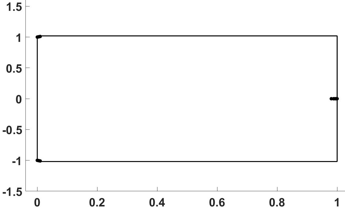
(a) $M^{-1}_{d}K$

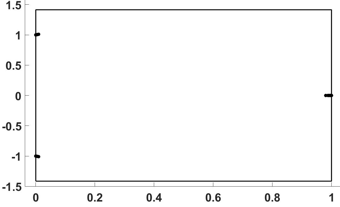
(b) $P^{-1}_{ibd}\check{K}$

Figure 1: Estimated ranges of eigenvalues of the preconditioned matrices $M^{-1}_{d}K=P^{-1}_{ibd}\check{K}$ for the case of $p=32$ in Example 6.1. Here each “exact” eigenvalue (or each cluster of eigenvalues) is marked by dot ‘·’, and the estimated bounds are marked by rectangles.

Remark 5.6.

Fig. 2 draws an example of the exact eigenvalues and the estimated eigenvalue bounds of the matrix $K$ preconditioned by preconditioners $M_{d}$, $M_{ut}$, $M_{lt}$, $M_{f_{1}}$ and $M_{f_{2}}$ all in the exact form. Here, the estimated eigenvalue bounds are in Table 3 of Corollary 5.3.

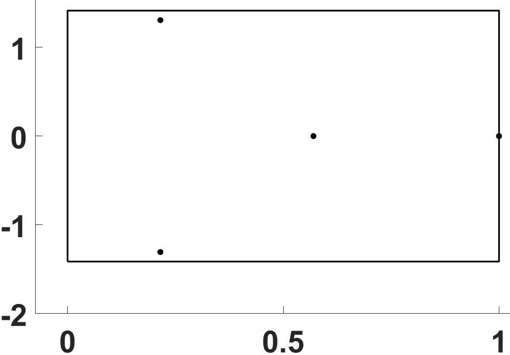
(a) $M^{-1}_{d}K$

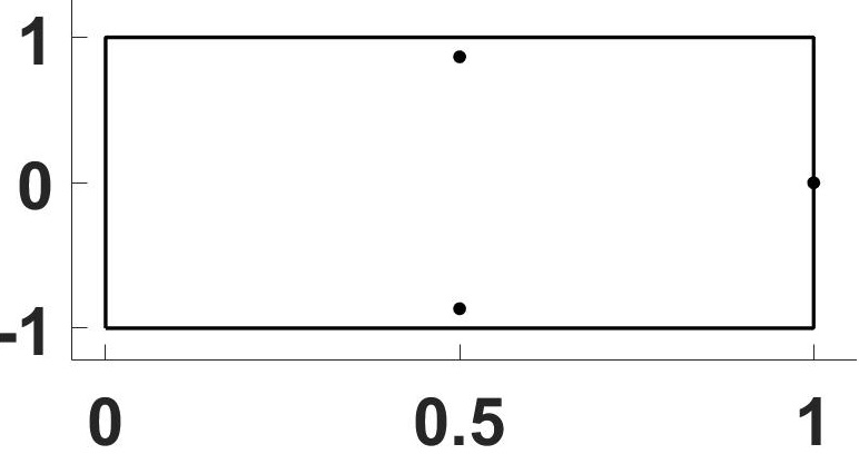
(b) $M^{-1}_{ut}K$

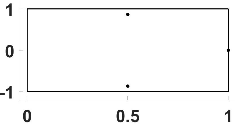
(c) $M^{-1}_{lt}K$

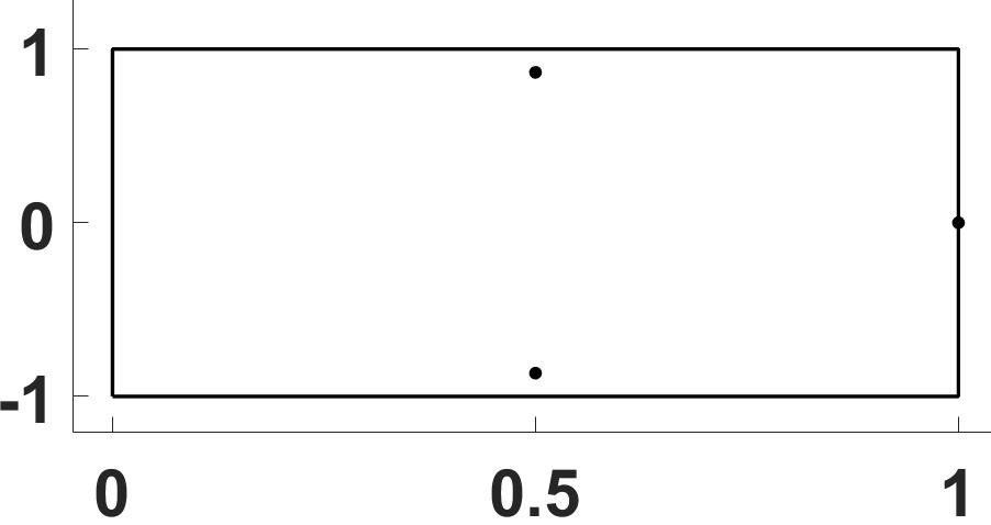
(d) $M^{-1}_{f_{1}}K$

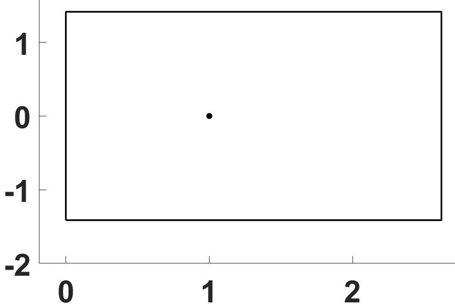
(e) $M^{-1}_{f_{2}}K$

Figure 2: Estimated ranges of eigenvalues of the matrix $K$ preconditioned by different exact preconditioners $M_{d}$, $M_{ut}$, $M_{lt}$, $M_{f_{1}}$ and $M_{f_{2}}$ for the case of $p=32$ in Example 6.1. Here each “exact” eigenvalue (or each cluster of eigenvalues) is marked by dot ‘·’, and the estimated bounds are marked by rectangles.

Since $\lambda=1$ is the unique eigenvalue of the preconditioned matrices $M^{-1}_{f_{3}}K$, $M^{-1}_{f_{4}}K$ and $M^{-1}_{f_{5}}K$, and since the estimated eigenvalue bounds, obtained in Table 3, are the exact ones, we did not draw them in Fig. 2.

In Fig. 2, rectangles mean the lower and upper bounds of the real and imaginary parts of the eigenvalues of the exact preconditioned matrix $M^{-1}_{*}K$ for each $*=d,ut,lt,f_{1},f_{2}$, and dots mean the “exact” eigenvalues or “cluster” of eigenvalues. We can find that the estimated upper bounds of the real parts of the eigenvalues of preconditioned matrices are almost sharp except $M^{-1}_{f_{2}}K$.

6 Numerical experiments

In this section, we present a list of numerical tests aiming at illustrating the efficiency of the proposed preconditioners Eqs. 70, 71, 72, 77, 73, 75, 76, and 74. We focus on solving two kinds of systems of linear equations, one with $D=0$ and the other with $D\neq 0$, by preconditioned-GMRES. The system of linear equations from five different test problems, which are used in [28, 48, 24, 21, 11, 12, 40].

To compare to the preconditioners proposed in Section 4, we gather eleven preconditioners used to solve systems of linear equations in the form of Eq. 1 or Eq. 2. For convenience, we abbreviate all corresponding preconditioned-GMRES as follows:

$P_{ebd}$-GMRES:	GMRES preconditioned by $P_{1}$, the exact block diagonal preconditioner in [28],
$P_{ibd}$-GMRES:	GMRES preconditioned by $P_{2}$, the inexact block diagonal preconditioner in [28],
$P_{1}$-GMRES:	GMRES preconditioned by the block preconditioner $P_{1}$ in [48],
$P_{2}$-GMRES:	GMRES preconditioned by the block preconditioner $P_{2}$ in [48],
$P_{3}$-GMRES:	GMRES preconditioned by the block preconditioner $P_{3}$ in [48],
$P_{ss}$-GMRES:	GMRES preconditioned by the shift-splitting preconditioner in [19],
$P_{rss}$-GMRES:	GMRES preconditioned by the relaxed shift-splitting preconditioner in [19],
$P_{ds}$-GMRES:	GMRES preconditioned by the dimensional split preconditioner in [11],
$P_{rdf}$-GMRES:	GMRES preconditioned by the relaxed dimensional factorization preconditioner in [12],
$P_{sdf}$-GMRES:	GMRES preconditioned by the stabilized dimensional factorization preconditioner in [25],
$P_{mal}$-GMRES:	GMRES preconditioned by the modified augmented Lagrangian preconditioner in [13],
$M_{*}$-GMRES:	GMRES preconditioned by the $M_{*}$ in Eqs. 70, 71, 72, 77, 73, 75, 76, and 74.

In the above list, the first seven preconditioned-GMRES are constructed in [28, 19, 48] to solve the system of linear equations in the form of Eq. 1 with $D=0$, the next four in [11, 12, 25, 13] to solve the system of linear equations in the form of Eq. 2 with $D\neq 0$, and those corresponding to the last one are new.

In the case of $D=0$, the new preconditioned-GMRES proposed in this paper and the first seven ones in the list are applied on the system in the form of Eq. 1. In the case of $D\neq 0$, the next four preconditioned-GMRES in the list are applied on the system in the form of Eq. 2, as in [11, 12, 25, 13], while the new ones proposed are applied on the equivalent system in the form of Eq. 1.

All numerical experiments are performed in MATLAB (version R2018a) and use the function gmres with the corresponding preconditioners on a personal computer, which has a 1.60-2.11GHz central processor (Intel(R) Core(TM) i5-10210u CPU) and 12G memory.

In the experiments, the initial point is set to be $x^{0}=0$, and IT, the number of iteration steps, and CPU, the CPU time cost in seconds, are recorded. We average the CPU for ten times and terminate the iteration once IT, the number of the iteration steps, exceeds 1000 or $RES\leq 10^{-6}$, where

$$RES=\frac{\parallel b-Kx^{k}\parallel_{2}}{\parallel b-Kx^{0}\parallel_{2}}.$$

6.1 The case of $D=0$

In this case, we’ll compare $M_{*}$-GMRES to the first seven preconditioned-GMRES in the above list for two modified systems of linear equations arising from two real problems.

In the numerical performance, all preconditioned-GMRES are used to solve the systems of linear equations in the form of Eq. 1. All the preconditioners, denoted by $M_{*}$ in Eqs. 70, 71, 72, 77, 73, 75, 76, and 74 and $P_{ibd}$ in [28] are inexact, and others are all exact. The parameter $\alpha$ needed in $P_{ss}$ and $P_{rss}$ are chosen as $\alpha=0.01$, the same as that in [19].

Example 6.1.

([28, 19, 48]) A modified system interfer with the Stokes problem. It is a modification of the system of linear equations arises in the Stokes problem [5].

Assume $A,B,C,D$ are defined by

$$A\!=\!\begin{pmatrix}I_{p}\!\otimes\!T_{p}\!+\!T_{p}\!\otimes\!I_{p}&\!\!0\\ 0&\!\!I_{p}\!\otimes\!T_{p}\!+\!T_{p}\!\otimes\!I_{p}\end{pmatrix}\!,\hskip 6.99997ptB\!=\!\begin{pmatrix}I_{p}\!\otimes\!F_{p}&\!\!F_{p}\!\otimes\!I_{p}\end{pmatrix},\hskip 6.99997ptC\!=\!E_{p}\otimes F_{p},\hskip 6.99997ptD\!=\!0$$

with

$$T_{p}\!=\!\frac{1}{h^{2}}\text{tridiag}(-1,2,-1),\hskip 8.00003ptF_{p}\!=\!\frac{1}{h}\text{tridiag}(0,1,-1),\hskip 8.00003ptE_{p}\!=\!\text{diag}(1,p+1,\cdots,p^{2}-p+1),$$

where $p$ is a positive integer, $h=\frac{1}{p+1}$ is the discretization mesh size, and $\otimes$ is the Kronecker product symbol.

It is easy to know that the matrix $A$ is SPD, that matrices $B$ and $C$ have full row rank, and that $n=2p^{2}$, $m=p^{2}$, $l=p^{2}$.

For inexact preconditioners $M_{*}$ in Eqs. 70, 71, 72, 77, 73, 75, 76, and 74 and $P_{ibd}$ in [28], the matrices $M_{A}$, $\widehat{S}$ and $\widehat{M}_{S}$ are chosen as

$$M_{A}=A,\hskip 15.00002pt\widehat{S}=BB^{T},\hskip 15.00002pt\widehat{M}_{S}=C\widehat{S}^{-1}C^{T}.$$

Table 4: IT and CPU in the form of “IT(CPU)” for different preconditioned-GMRES.

Method	$p=32$	$p=64$	$p=96$
$P_{ebd}$-GMRES	4(1.157)	4(75.954)	4(822.431)
$P_{ibd}$-GMRES	8(1.106)	8(27.687)	8(217.129)
$P_{ss}$-GMRES	3(0.254)	3(2.565)	3(20.246)
$P_{rss}$-GMRES	3(0.263)	3(2.502)	3(20.481)
$P_{1}$-GMRES	3(1.028)	3(35.436)	3(392.035)
$P_{2}$-GMRES	3(1.010)	3(35.623)	3(392.891)
$P_{3}$-GMRES	2(0.949)	2(27.454)	2(606.317)
$M_{d}$-GMRES	9(1.198)	8(27.497)	8(214.460)
$M_{ut}$-GMRES	7(0.988)	7(24.995)	7(195.506)
$M_{lt}$-GMRES	7(1.027)	7(24.791)	7(196.801)
$M_{f_{1}}$-GMRES	7(2.814)	7(79.275)	7(831.203)
$M_{f_{2}}$-GMRES	3(0.024)	3(0.126)	3(0.349)
$M_{f_{3}}$-GMRES	2(0.018)	2(0.067)	2(0.172)
$M_{f_{4}}$-GMRES	2(0.019)	2(0.070)	2(0.207)
$M_{f_{5}}$-GMRES	2(0.134)	2(2.417)	2(13.055)

Table 4 lists IT and CPU in the form of “IT(CPU)” for each preconditioned-GMRES for solving systems with $p=32,64,96$. From Table 4, we can find that $M_{f_{2}}$-GMRES, $M_{f_{3}}$-GMRES, $M_{f_{4}}$-GMRES and $M_{f_{5}}$-GMRES require less numbers of iteration steps or less CPU times than all the other tested preconditioned-GMRES. So, $M_{f_{3}}$-GMRES seems to be much better among them since both the numbers of iteration steps and the CPU times required are less. In other words, $M_{f_{3}}$-GMRES is best among these fifteen preconditioned-GMRES tested and listed in Table 4.

We can also find that, for $M_{ut}$-GMRES and $M_{lt}$-GMRES, the numbers of iteration steps and the CPU time are both better than that of $P_{ibd}$-GMRES, and that the CPU time is better than that of $P_{ebd}$-GMRES, $P_{1}$-GMRES, $P_{2}$-GMRES and $P_{3}$-GMRES. $M_{d}$-GMRES needs less CPU time than $P_{ebd}$-GMRES, $P_{ibd}$-GMRES, $P_{1}$-GMRES, $P_{2}$-GMRES and $P_{3}$-GMRES as $p$ becomes greater.

Example 6.2.

([28, 48]) A modified system interfer with the optimization problem. It is a modification of the system of linear equations arises in computing the descent directions in the Newton steps involved in the modified primal–dual interior point method used to solve the nonsmooth and nonconvex minimization problems from restorations of piecewise constant images [33, 1].

Suppose $p$ is a positive integer, $\widetilde{p}=p^{2}$ and $\widehat{p}=p(p+1)$. Assume $A,B,C,D$ are defined by

$$A=Diag(2W^{T}W\!+\!I_{\widehat{p}},D_{1},D_{2}),\hskip 10.00002ptB=(E,-I_{2\widetilde{p}},-I_{2\widetilde{p}}),\hskip 10.00002ptC=E^{T},\hskip 10.00002ptD=0$$

with

$$W=(w_{ij})_{\widehat{p}},\hskip 8.00003ptD_{1}=diag(d^{(1)}_{j})_{2\widetilde{p}},\hskip 8.00003ptD_{2}=diag(d^{(2)}_{j})_{2\widetilde{p}},\hskip 8.00003ptE=\begin{pmatrix}\widehat{E}\otimes I_{p}\\ I_{p}\otimes\widehat{E}\end{pmatrix},$$

where $\otimes$ is the Kronecker product symbol and

$$\ \ \begin{array}[]{l}w_{ij}=e^{-2((i/3)^{2}+(j/3)^{2})},\hskip 2.5pt\text{for}\ 1\leq i,j\leq\widehat{p},\\ d^{(1)}_{j}=\begin{cases}1,&\text{for}\ 1\leq j\leq\widetilde{p},\\ 10^{-5}(j-\widetilde{p})^{2},&\text{for}\ \widetilde{p}+1\leq j\leq 2\widetilde{p},\end{cases}\\ d^{(2)}_{j}=10^{-5}(j+\widetilde{p})^{2},\hskip 16.49995pt\text{for}\ 1\leq j\leq 2\widetilde{p},\end{array}\hskip 5.0pt\widehat{E}=\!\begin{pmatrix}2&-1&&&\\ &2&-1&&\\ &&\ddots&\ddots&\\ &&&2&-1\end{pmatrix}_{\!p\times(p\!+\!1)}\!\!\!\!\!\!\!.$$

It is easy to know that the matrix $A$ is SPD, matrices $B$ and $C$ have full row rank, and $n=5p^{2}+p$, $m=2p^{2}$, $l=p^{2}+p$.

For inexact preconditioners $M_{*}$ in Eqs. 70, 71, 72, 77, 73, 75, 76, and 74 and $P_{ibd}$ in [28], the matrices $M_{A}$, $\widehat{S}$ and $\widehat{M}_{S}$ are chosen as

$$M_{A}=LL^{T},\hskip 15.00002pt\widehat{S}=diag(BM^{-1}_{A}B^{T}),\hskip 15.00002pt\widehat{M}_{S}=C\widehat{S}^{-1}C^{T},$$

where $L$ is produced by the incomplete Cholesky decomposition of $A$ with the droptol being $10^{-8}$, the same selection as in [28].

Table 5: IT and CPU in the form of “IT(CPU)” for different preconditioned-GMRES.

Method	$p=40$	$p=60$	$p=80$
$P_{ebd}$-GMRES	6(2.242)	6(15.325)	6(62.219)
$P_{ibd}$-GMRES	82(0.247)	104(0.776)	92(2.083)
$P_{ss}$-GMRES	4(0.131)	4(0.307)	4(0.562)
$P_{rss}$-GMRES	3(0.104)	3(0.246)	3(0.441)
$P_{1}$-GMRES	3(2.371)	3(15.260)	3(60.364)
$P_{2}$-GMRES	3(2.337)	3(15.327)	3(62.075)
$P_{3}$-GMRES	3(1.232)	3(8.220)	3(33.615)
$M_{d}$-GMRES	47(0.352)	52(0.990)	72(2.217)
$M_{ut}$-GMRES	40(0.305)	44(0.732)	46(1.397)
$M_{lt}$-GMRES	34(0.258)	38(0.572)	40(1.102)
$M_{f_{1}}$-GMRES	104(3.647)	114(8.692)	109(14.752)
$M_{f_{2}}$-GMRES	10(0.098)	10(0.239)	10(0.451)
$M_{f_{3}}$-GMRES	8(0.178)	9(0.463)	9(0.818)
$M_{f_{4}}$-GMRES	2(0.071)	2(0.156)	2(0.303)
$M_{f_{5}}$-GMRES	2(0.125)	2(0.282)	2(0.535)

Table 5 lists IT and CPU in the form of “IT(CPU)” for each preconditioned-GMRES for solving systems with $p=40,60,80$. From Table 5, we can find that $M_{f_{4}}$-GMRES and $M_{f_{5}}$-GMRES require less numbers of iteration steps or less CPU times than all the other tested preconditioned-GMRES. In these two preconditioned-GMRES, $M_{f_{4}}$-GMRES seems to be much better since both the numbers of iteration steps and the CPU times required are less. In other words, $M_{f_{4}}$-GMRES is best among these fifteen preconditioned-GMRES tested and listed in Table 5.

Moreover, we can see from Table 5 that $M_{f_{2}}$-GMRES is superior to all compared preconditioned-GMRES in CPU time except $P_{rss}$-GMRES when $p=80$, that $M_{f_{3}}$-GMRES is superior to all comparison preconditioned-GMRES in CPU time except $P_{ss}$-GMRES and $P_{rss}$-GMRES, and that $M_{f_{2}}$-GMRES and $M_{f_{3}}$-GMRES are better than $P_{ibd}$-GMRES for the number of iteration steps.

In addition, from Table 5, we can know that $M_{d}$-GMRES, $M_{ut}$-GMRES and $M_{lt}$-GMRES cost less CPU times compared to $P_{ebd}$-GMRES, $P_{1}$-GMRES, $P_{2}$-GMRES and $P_{3}$-GMRES. So do $M_{ut}$-GMRES and $M_{lt}$-GMRES compared to $P_{ibd}$-GMRES when $p=60$ and $p=80$. Compared to $P_{1}$-GMRES, $P_{2}$-GMRES, and $P_{3}$-GMRES, $M_{f_{1}}$-GMRES also needs less CPU time as $p$ becomes greater.

Examples 6.2 and 6.1 show us that, in the case of $D=0$, preconditioners $M_{f_{4}}$ and $M_{f_{5}}$ have higher efficiency in all numerical tests, and that $M_{f_{2}}$ and $M_{f_{3}}$ play well in most of tests compared to five preconditioners $P_{ebd}$, $P_{ibd}$, $P_{1}$, $P_{2}$ and $P_{3}$. In addition, the other four proposed preconditioners have superiority in the number of iteration steps or CPU time in some tests.

6.2 The case of $D\neq 0$

In this case, we’ll compare $M_{*}$-GMRES to the $P_{ds}$-GMRES, $P_{rdf}$-GMRES, $P_{sdf}$-GMRES and $P_{mal}$-GMRES in the list for systems of linear equations coming from three real problems.

In numerical performance of this case, $P_{ds}$-GMRES, $P_{rdf}$-GMRES, $P_{mal}$-GMRES and $P_{sdf}$-GMRES are used to solve the systems of linear equations in the form of Eq. 2, while $M_{*}$-GMRES is used to solve the equivalent systems in the form of Eq. 1 for each suitable $``*"$.

The matrix $W$ appeared in $P_{sdf}$ is chosen as $W=diag(\mathfrak{B}\mathfrak{B^{T}})$ [25], and matrices $W$ and $\widehat{S}$ appeared in $P_{mal}$ are chosen as $W=-\alpha\widehat{S}=diag(\mathfrak{B}\mathfrak{A^{-1}}\mathfrak{B^{T}})$ [13], where

$$\mathfrak{A}=\begin{pmatrix}A&0\\ 0&D\end{pmatrix},\hskip 10.00002pt\mathfrak{B}=\begin{pmatrix}B&C^{T}\end{pmatrix}.$$

The only parameter, denoted by $\alpha$, needed necessarily in $P_{ds}$-GMRES, $P_{rdf}$-GMRES, $P_{sdf}$-GMRES and $P_{mal}$-GMRES are chosen in the interval $(0,50)$ since numerical tests in [11] and [12] indicate that the best results are obtained for smaller $\alpha$.

The parameter $\alpha$ is chosen as well as possible in four steps. At first, we record the numbers of iteration steps for each preconditioned-GMRES at all nodes in the interval with step size $1$, and obtain a proper sub-interval $[a,b](a\leq b)$ in which the numbers of iteration steps at all nodes reach the minimization. Next, we carry out experiments for all new nodes in the interval $(0,10h]\cup[a-9h,b+9h]$ with step size $h=0.1$. Then, we repeat the process with step size $h=0.01$, $0.001$ in turn until the step size $h$ reaches $0.001$ or the number of iteration steps at each node belonging to $[a,b]$ equals the minimal number of iteration steps at all nodes in $[a-9h,b+9h]$. Finally, we denote by $\alpha_{opt}$ the parameter node which belongs to the last interval $[a,b]$ and makes simultaneously both the number of iteration steps and the CPU time least, and call it the “numerical optimal parameter”.

Example 6.3.

A quadratic program with equality constraints. This kind of system of linear equations arises from the quadratic program with equality constraints, named as AUG3DC with the number of nodes in the corresponding direction (named as NND for simplicity), in the CUTEr collection [24].

The original system of linear equations is in the form of Eq. 2. In the system, matrices $A$ and $D$ are both SPD, and the matrix $B$ has full row rank.

In this example, the NND is chosen as $15$, $20$ and $25$, respectively. For preconditioners denoted by $M_{*}$ in Eqs. 70, 71, 72, 77, 73, 75, 76, and 74, matrices $M_{A}$, $\widehat{S}$ and $\widehat{M}_{S}$ are chosen as

$$M_{A}=A,\hskip 10.00002pt\widehat{S}=BM_{A}^{-1}B^{T}+0.1I,\hskip 10.00002pt\widehat{M}_{S}=D+C\widehat{S}^{-1}C^{T}.$$

Table 6 lists the numerical optimal parameter $\alpha_{opt}$, and IT and CPU in the form of “IT(CPU)” for each preconditioned-GMRES (at $\alpha_{opt}$ if needed).

Table 6: IT and CPU in the form of “IT(CPU)” and $\alpha_{opt}$ for different preconditioned-GMRES.

Method	NND=$15$		NND=$20$		NND=$25$
	$\alpha_{opt}$	IT(CPU)	$\alpha_{opt}$	IT(CPU)	$\alpha_{opt}$	IT(CPU)
$P_{ds}$-GMRES	0.59	20(1.262)	0.41	21(4.000)	0.32	22(11.373)
$P_{rdf}$-GMRES	0.8	15(0.986)	0.43	17(3.189)	0.31	19(9.585)
$P_{sdf}$-GMRES	0.09	14(0.926)	0.075	16(3.032)	0.04	19(9.596)
$P_{mal}$-GMRES	9.2	14(1.342)	15	17(5.256)	21	19(21.883)
$M_{d}$-GMRES	$--$	44(66.979)	$--$	47(266.702)	$--$	56(913.062)
$M_{ut}$-GMRES	$--$	45(68.502)	$--$	45(255.672)	$--$	51(856.850)
$M_{lt}$-GMRES	$--$	43(67.787)	$--$	46(261.111)	$--$	51(859.511)
$M_{f_{1}}$-GMRES	$--$	44(67.065)	$--$	45(255.084)	$--$	50(830.257)
$M_{f_{2}}$-GMRES	$--$	22(0.525)	$--$	23(1.829)	$--$	25(6.405)
$M_{f_{3}}$-GMRES	$--$	7(0.285)	$--$	8(1.015)	$--$	9(3.285)
$M_{f_{4}}$-GMRES	$--$	7(0.275)	$--$	8(0.985)	$--$	9(3.143)
$M_{f_{5}}$-GMRES	$--$	6(0.185)	$--$	7(0.971)	$--$	8(2.625)

       $``--"$ means that $\alpha_{opt}$ is not required.

From Table 6, we can find that $M_{f_{2}}$-GMRES, $M_{f_{3}}$-GMRES, $M_{f_{4}}$-GMRES and $M_{f_{5}}$-GMRES require less numbers of iteration steps or less CPU times than all the other tested preconditioned-GMRES. Among these four preconditioned-GMRES, $M_{f_{5}}$-GMRES seems to be much better since both the numbers of iteration steps and the CPU times required are less. In other words, $M_{f_{5}}$-GMRES is the best compared to all other eleven preconditioned-GMRES listed in Table 6. For this example, $M_{d}$, $M_{ut}$, $M_{lt}$ and $M_{f_{1}}$, the other four preconditioners proposed in this paper, are mediocre for accelerating GMRES compared to $P_{ds}$, $P_{rdf}$, $P_{sdf}$ and $P_{mal}$.

Example 6.4.

The leaky lid driven cavity problem. This kind of system of linear equations are generated from the discretization of the incompressible Stokes flow problem described by

(90) $$\begin{array}[]{rl}-\bigtriangledown^{2}\textbf{u}+\bigtriangledown p=\textbf{0}&\text{in}\ \Omega,\\ \bigtriangledown\cdot\textbf{u}=0&\text{in}\ \Omega,\\ \textbf{u}=\textbf{0}&\text{on}\ \partial\Omega\backslash\partial\Omega_{lid},\\ \textbf{u}_{x}=1&\text{on}\ \partial\Omega_{lid}\end{array}\hskip 10.00002pt\text{with}\hskip 10.00002pt\begin{array}[]{l}\Omega=(-1,1)\times(-1,1),\\ \partial\Omega_{lid}=[-1,1]\times\{1\},\end{array}$$

and $\textbf{u}=(\textbf{u}_{x},\textbf{u}_{y})$ is a vector-valued function representing the velocity of the fluid, and the scalar function $p$ represents the pressure.

Three discretization systems of Eq. 90 in the form of Eq. 2 are generated via IFISS software package [21] by using Q2-Q1 finite elements on the uniform grids with $32\times 32$, $64\times 64$ and $128\times 128$ meshes, respectively. In these three discretization systems, $A$, $D$ are SPD and $B$ has full row rank.

For each preconditioner $M_{*}$ in Eqs. 70, 71, 72, 77, 73, 75, 76, and 74, the matrices $M_{A}$, $\widehat{S}$ and $\widehat{M}_{S}$ are

$$M_{A}=A,\hskip 15.00002pt\widehat{S}=BM^{-1}_{A}B^{T}+0.01diag(BM^{-1}_{A}B^{T}),\hskip 15.00002pt\widehat{M}_{S}=D+C\widehat{S}^{-1}C^{T}.$$

Table 7: IT and CPU in the form of “IT(CPU)” and $\alpha_{opt}$ for different preconditioned-GMRES.

Method	$32\times 32$		$64\times 64$		$128\times 128$
	$\alpha_{opt}$	IT(CPU)	$\alpha_{opt}$	IT(CPU)	$\alpha_{opt}$	IT(CPU)
$P_{ds}$-GMRES	0.001	15(0.489)	0.001	26(6.571)	0.001	48(165.108)
$P_{rdf}$-GMRES	0.001	15(0.496)	0.001	21(5.398)	49.92	13(25.107)
$P_{sdf}$-GMRES	0.22	10(0.345)	0.19	11(2.719)	0.22	11(37.148)
$P_{mal}$-GMRES	2.4	12(0.537)	2.8	12(3.553)	2.0	13(24.361)
$M_{d}$-GMRES	$--$	45(4.458)	$--$	55(167.196)	$--$	$--$
$M_{ut}$-GMRES	$--$	48(5.174)	$--$	55(181.419)	$--$	$--$
$M_{lt}$-GMRES	$--$	29(3.063)	$--$	38(118.627)	$--$	$--$
$M_{f_{1}}$-GMRES	$--$	29(2.897)	$--$	36(108.328)	$--$	$--$
$M_{f_{2}}$-GMRES	$--$	24(0.587)	$--$	24(8.829)	$--$	24(216.108)
$M_{f_{3}}$-GMRES	$--$	4(0.142)	$--$	4(2.493)	$--$	4(62.394)
$M_{f_{4}}$-GMRES	$--$	3(0.128)	$--$	3(1.679)	$--$	3(41.105)
$M_{f_{5}}$-GMRES	$--$	3(0.050)	$--$	3(0.239)	$--$	3(1.510)

$``--"$ means that $\alpha_{opt}$ is not required or that the CPU time exceeds 1000 seconds.

Table 7 lists the numerical optimal parameter $\alpha_{opt}$, and IT and CPU in the form of “IT(CPU)” for different preconditioned-GMRES (at $\alpha_{opt}$ if needed) for the incompressible Stokes problem discretized on different meshes. Table 7 shows us that for this example, less numbers of iteration steps or less CPU times are needed in the case of using $M_{f_{3}}$-GMRES, $M_{f_{4}}$-GMRES and $M_{f_{5}}$-GMRES. Among these three preconditioned-GMRES, $M_{f_{5}}$-GMRES seems to be much better since both the numbers of iteration steps and the CPU times required are less as mesh becomes dense. In other words, $M_{f_{5}}$-GMRES is the best compared to all other eleven preconditioned-GMRES listed in Table 7. We can see that, for this example, $M_{d}$, $M_{ut}$, $M_{lt}$, $M_{f_{1}}$ and $M_{f_{2}}$, are mediocre for accelerating GMRES compared to $P_{ds}$, $P_{rdf}$, $P_{mal}$ and $P_{sdf}$.

The eigenvalue distributions and the estimated eigenvalue bounds, obtained in Theorem 5.1, about the preconditioned matrices with proposed preconditioners $M_{*}$ in Eqs. 70, 71, 72, 77, 73, 75, 76, and 74, are drawn in Fig. 3 for $32\times 32$ meshes. In Fig. 3, rectangles mean the lower and upper bounds of the real and imaginary parts of the eigenvalues of the preconditioned matrix $M^{-1}_{*}K$ for $*=d,ut,lt,f_{1},f_{2},f_{3},f_{4},f_{5}$, and dots mean the “exact” or clusters of eigenvalues.

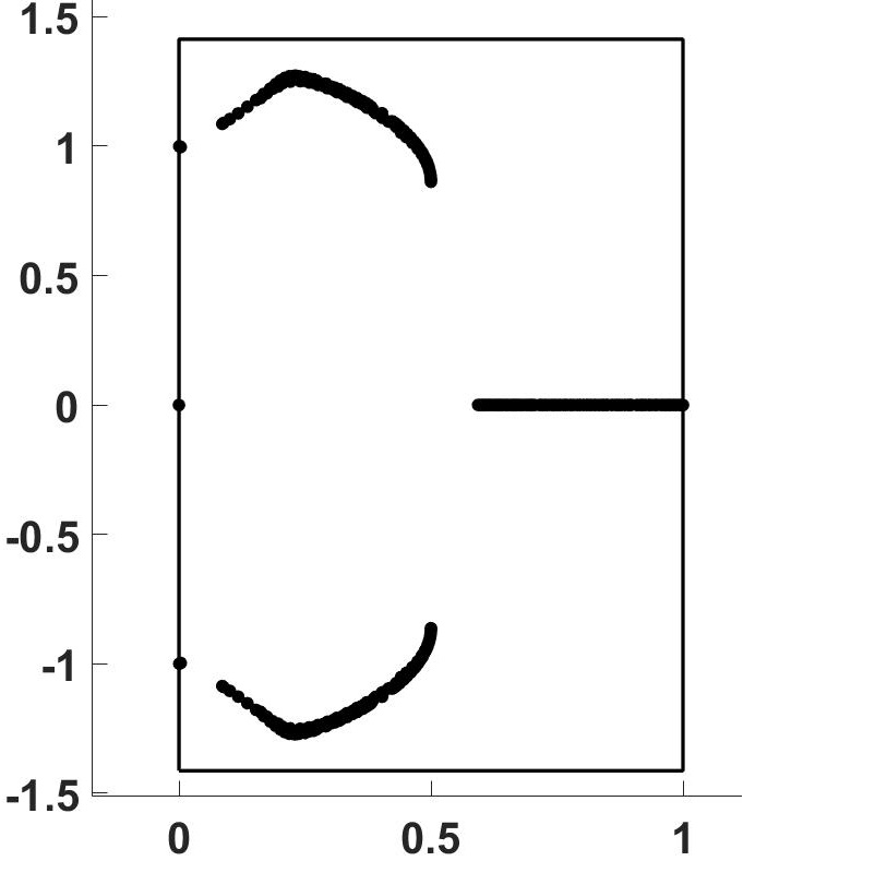
(a) $M^{-1}_{d}K$

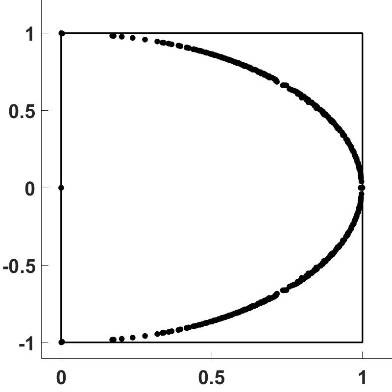
(b) $M^{-1}_{ut}K$

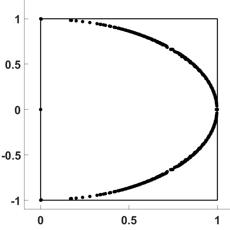
(c) $M^{-1}_{lt}K$

(d) $M^{-1}_{f_{1}}K$

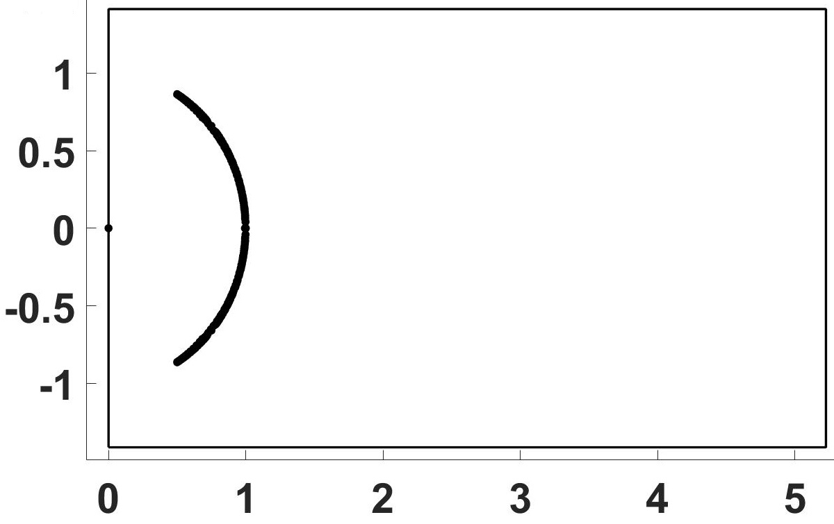
(e) $M^{-1}_{f_{2}}K$

(f) $M^{-1}_{f_{3}}K$

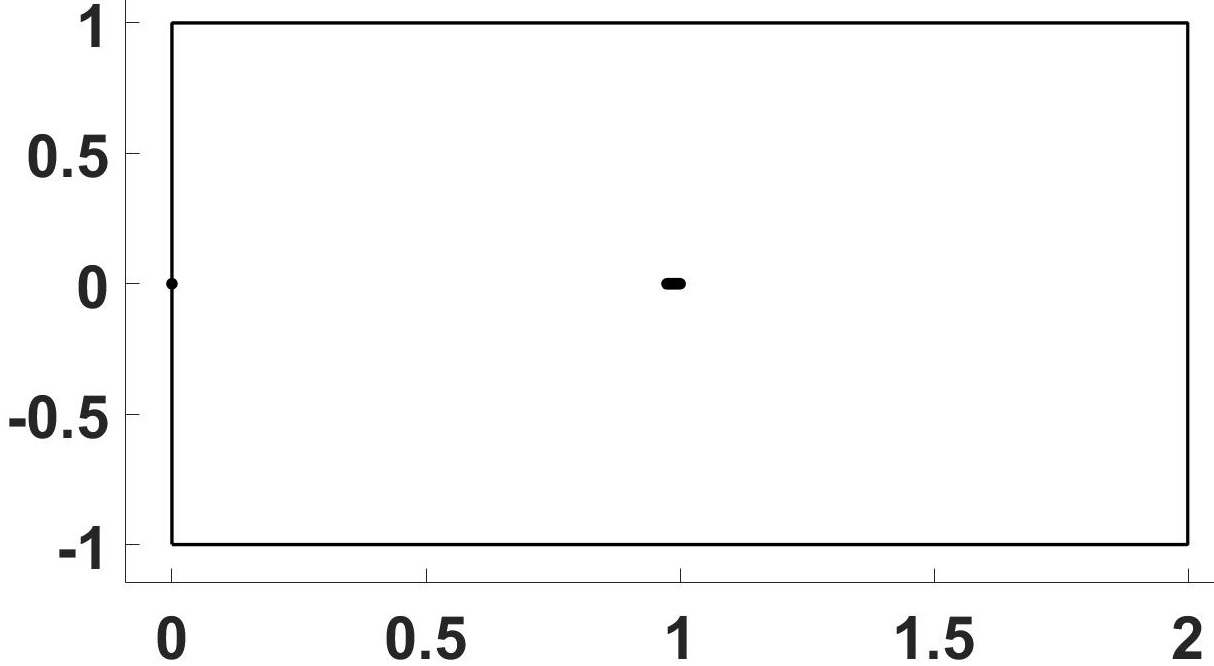
(g) $M^{-1}_{f_{4}}K$

(h) $M^{-1}_{f_{5}}K$

Figure 3: Estimated ranges of eigenvalues of the preconditioned matrix $M^{-1}_{*}K$ for $32\times 32$ meshes in Example 6.4. Here each “exact” or each cluster of eigenvalue is marked by dot ‘·’, and the estimated bounds are marked by rectangles.

From Fig. 3, we can observe that $M^{-1}_{f_{3}}K$, $M^{-1}_{f_{4}}K$ and $M^{-1}_{f_{5}}K$ gather eigenvalues near $0$ and $1$, and that the estimated bounds of the eigenvalues are sharp for $M^{-1}_{d}K$, $M^{-1}_{ut}K$, $M^{-1}_{lt}K$ and $M^{-1}_{f_{1}}K$. Moreover, the estimated lower bounds of the real parts of the eigenvalues are sharp for $M^{-1}_{f_{2}}K$, $M^{-1}_{f_{3}}K$, $M^{-1}_{f_{4}}K$ and $M^{-1}_{f_{5}}K$.

Example 6.5.

([40]) The Poisson control problem. This kind of system of linear equations are generated from the discretization of the distributed control problem with Dirichlet boundary conditions defined by

$$\min\limits_{u,f}\frac{1}{2}\parallel u-\hat{u}\parallel^{2}_{L_{2}(\Omega)}+\frac{\beta}{2}\parallel f\parallel^{2}_{L_{2}(\Omega)}$$

s.t. $$\begin{array}[]{rl}-\bigtriangledown^{2}{u}={f}&\text{in}\ \Omega,\\ u=g&\text{on}\ \partial\Omega,\end{array}$$

where $u$ is the state, $\hat{u}$ is the desired state, $0<\beta\ll 1$ is a regularization parameter, $f$ is the control, and $\omega$ is the domain with boundary $\partial\Omega$.

Three systems of linear equations in the form of Eq. 2 are generated automatically by the MATLAB code, used in [40], download from [39], after parameters in “set_def_setup.m” are selected as def_setup.bc = ‘dirichlet’, def_setup.beta = 1e-2, def_setup.ob = 1, def_setup.type = ‘dist2d’ and def_setup.pow = 5, 6 and 7. In these three systems, $A$ and $D$ are SPD, $C$ and $B$ have full row rank.

In this example, for each preconditioner $M_{*}$ in Eqs. 70, 71, 72, 77, 73, 75, 76, and 74, matrices $M_{A}$, $\widehat{S}$ and $\widehat{M}_{S}$ are taken by

$$M_{A}=LL^{T},\hskip 15.00002pt\widehat{S}=tridiag(BM^{-1}_{A}B^{T}),\hskip 15.00002pt\widehat{M}_{S}=D+C\widehat{S}^{-1}C^{T},$$

where $L$ is produced by the incomplete Cholesky decomposition of $A$ with the droptol being $10^{-8}$, $tridiag(\cdot)$ is the tridiagonal matrix whose tridiagonal part consists of the tridiagonal entries of the corresponding matrix in turn.

Table 8: IT and CPU in the form of “IT(CPU)” and $\alpha_{opt}$ for different preconditioned-GMRES.

Method	def_setup.pow = 5		def_setup.pow = 6		def_setup.pow = 7
	$\alpha_{opt}$	IT(CPU)	$\alpha_{opt}$	IT(CPU)	$\alpha_{opt}$	IT(CPU)
$P_{ds}$-GMRES	0.001	20(0.721)	0.002	59(29.123)	0.002	111(373.931)
$P_{rdf}$-GMRES	0.2	7(0.271)	0.1	7(3.583)	0.016	6(18.071)
$P_{sdf}$-GMRES	0.02	7(0.267)	0.01	7(3.746)	0.003	6(18.467)
$P_{mal}$-GMRES	0.001	18(0.834)	0.001	10(4.160)	0.001	14(115.288)
$M_{d}$-GMRES	$--$	49(1.262)	$--$	47(18.681)	$--$	47(434.678)
$M_{ut}$-GMRES	$--$	20(0.609)	$--$	20(8.587)	$--$	18(103.551)
$M_{lt}$-GMRES	$--$	48(1.397)	$--$	65(27.572)	$--$	69(630.851)
$M_{f_{1}}$-GMRES	$--$	20(4.439)	$--$	20(128.855)	$--$	$--$
$M_{f_{2}}$-GMRES	$--$	8(0.126)	$--$	8(0.641)	$--$	8(315.389)
$M_{f_{3}}$-GMRES	$--$	3(0.195)	$--$	3(1.658)	$--$	3(12.057)
$M_{f_{4}}$-GMRES	$--$	4(0.221)	$--$	4(2.553)	$--$	4(12.151)
$M_{f_{5}}$-GMRES	$--$	3(1.716)	$--$	3(71.853)	$--$	$--$

     $``--"$ means that $\alpha_{opt}$ is not required or that the CPU time exceeds 1000 seconds.

Table 8 lists the numerical optimal parameter $\alpha_{opt}$, and IT and CPU in the form of “IT(CPU)” for different preconditioned-GMRES (at $\alpha_{opt}$ if needed) for the Poisson control problem. In Table 8, less numbers of iteration steps or less CPU times are needed in the case of using $M_{f_{3}}$-GMRES and $M_{f_{4}}$-GMRES than all the other tested preconditioned-GMRES. Compared to $P_{ds}$-GMRES, $M_{d}$-GMRES needs less number of iteration steps when def_setup.pow = 6 and 7, and $M_{ut}$-GMRES has superiority in the number of iteration steps and CPU time. $M_{f_{2}}$-GMRES and $M_{f_{5}}$-GMRES play well when def_setup.pow = 5 and 6, while spend much CPU time when def_setup.pow = 7.

Examples 6.3, 6.4, and 6.5 show us that, in the case of $D\neq 0$, preconditioners $M_{f_{3}}$ and $M_{f_{4}}$ have higher efficiency in all numerical tests, and that $M_{f_{5}}$ plays well in most of tests. So, the efficiency of these preconditioners suggests it is reasonable and beneficial to transform the system Eq. 2 into the equivalent one in the form of Eq. 1. In addition, the other five proposed preconditioners are mediocre in this case even though they play not bad in the case of $D=0$.

7 Conclusions

In this paper, by making use of the three-by-three block structure of the coefficient matrix, we have introduced eight inexact block factorization preconditioners based on a kind of inexact factorization for the coefficient matrix of the system of linear equations in the form of Eq. 1. The bounds of the real and imaginary parts of eigenvalues of the preconditioned matrices have been obtained based on our generalizing Bendixson Theorem and developing a unified technique of spectral equivalence. Numerical experiments on test problems show us that the proposed preconditioner $M_{f_{4}}$ is very efficient and can lead to high-speed and effective preconditioned-GMRES, and that preconditioners $M_{f_{3}}$ and $M_{f_{5}}$ play well in most of cases. The other five preconditioners are mediocre for accelerating GMRES in the case of $D\neq 0$, and are comparable in the case of $D=0$. The efficiency of $M_{f_{3}}$, $M_{f_{4}}$ and $M_{f_{5}}$ appeared in most of tests shows that it is reasonable and beneficial to convert the system Eq. 2 into the equivalent one of type Eq. 1.

As we can see in Section 4, the reason why we take these eight preconditioners into consideration together is that they are in a similar structure and have similar characteristics in theoretical analysis so that they can be put into a same theoretical frame, even if there are five preconditioners do not lead to much greater efficiency in the case of $D\neq 0$. Of cause, as mentioned in [9], “it is quite possible that some of the methods that were found to be not competitive for these test problems considered here may well turn out to be useful on other problems and, conversely, some of the methods found to be effective here may well perform poorly on other problems”.

References

- [1] Z.-Z. Bai, Optimal parameters in the HSS-like methods for saddle-point problems, Numer. Linear Algebra Appl., 16 (2009), pp. 447–479.
- [2] Z.-Z. Bai, Block preconditioners for elliptic PDE-constrained optimization problems, Computing, 91 (2011), pp. 379–395.
- [3] Z.-Z. Bai, M. Benzi, F. Chen, and Z.-Q. Wang, Preconditioned MHSS iteration methods for a class of block two-by-two linear systems with applications to distributed control problems, IMA J. Numer. Anal., 33 (2013), pp. 343–369.
- [4] Z.-Z. Bai, F. Chen, and Z.-Q. Wang, Additive block diagonal preconditioning for block two-by-two linear systems of skew-Hamiltonian coefficient matrices, Numer. algorithms, 62 (2013), pp. 655–675.
- [5] Z.-Z. Bai, G. H. Golub, and J.-Y. Pan, Preconditioned Hermitian and skew-Hermitian splitting methods for non-Hermitian positive semidefinite linear systems, Numer. Math., 98 (2004), pp. 1–32.
- [6] Z.-Z. Bai and M. Tao, Rigorous convergence analysis of alternating variable minimization with multiplier methods for quadratic programming problems with equality constraints, BIT Numer. Math., 56 (2016), pp. 399–422.
- [7] Z.-Z. Bai and M. Tao, On preconditioned and relaxed AVMM methods for quadratic programming problems with equality constraints, Linear Algebra Appl., 516 (2017), pp. 264–285.
- [8] A. T. Barker, T. Rees, and M. Stoll, A fast solver for an H1 regularized PDE-constrained optimization problem, Commun. Comput. Phys., 19 (2016), pp. 143–167.
- [9] F. P. A. Beik and M. Benzi, Iterative methods for double saddle point systems, SIAM J. Matrix Anal. Appl., 39 (2018), pp. 902–921.
- [10] M. Benzi, G. H. Golub, and J. Liesen, Numerical solution of saddle point problems, Acta Numer., 14 (2005), pp. 1–137.
- [11] M. Benzi and X.-P. Guo, A dimensional split preconditioner for Stokes and linearized Navier–Stokes equations, Appl. Numer. Math., 61 (2011), pp. 66–76.
- [12] M. Benzi, M. Ng, Q. Niu, and Z. Wang, A Relaxed Dimensional Factorization preconditioner for the incompressible Navier-Stokes equations, J. Comput. Phys., 230 (2011), pp. 6185–6202.
- [13] M. Benzi, M. A. Olshanskii, and Z. Wang, Modified augmented Lagrangian preconditioners for the incompressible Navier-Stokes equations, Int. J. Numer. Meth. Fl., 66 (2011), pp. 486–508.
- [14] M. Benzi and V. Simoncini, On the eigenvalues of a class of saddle point matrices, Numer. Math., 103 (2006), pp. 173–196.
- [15] A. Björck, Numerical Methods for Least Squares Problems, SIAM, Philadelphia, PA., 1996.
- [16] S. Bradley and C. Greif, Eigenvalue bounds for double saddle-point systems, arXiv preprint arXiv:2110.13328, (2021).
- [17] J. R. Bunch and B. N. Parlett, Direct methods for solving symmetric indefinite systems of linear equations, SIAM J. Numer. Anal., 8 (1971), pp. 639–655.
- [18] M.-C. Cai, G.-L. Ju, and J.-Z. Li, Schur complement based preconditioners for twofold and block tridiagonal saddle point problems, arXiv preprint arXiv:2108.08332, (2021).
- [19] Y. Cao, Shift-splitting preconditioners for a class of block three-by-three saddle point problems, Appl. Math. Lett., 96 (2019), pp. 40–46.
- [20] Z.-M. Chen, Q. Du, and J. Zou, Finite element methods with matching and nonmatching meshes for Maxwell equations with discontinuous coefficients, SIAM J. Numer. Anal., 37 (2000), pp. 1542–1570.
- [21] H. C. Elman, A. Ramage, and D. J. Silvester, Algorithm 866: IFISS, a matlab toolbox for modelling incompressible flow, ACM Trans. Math. Softw., 33 (2007), pp. 14–es.
- [22] G. N. Gatica and N. Heuer, An expanded mixed finite element approach via a dual–dual formulation and the minimum residual method, J. Comput. Appl. Math., 132 (2001), pp. 371–385.
- [23] G. N. Gatica and N. Heuer, Conjugate gradient method for dual-dual mixed formulations, Math. Comput., 71 (2002), pp. 1455–1472.
- [24] N. I. M. Gould, D. Orban, and P. L. Toint, CUTEr and SifDec, a constrained and unconstrained testing environment, revisited, ACM Trans. Math. Softw, 29 (2003), pp. 373–394.
- [25] L. Grigori, Q. Niu, and Y.-X. Xu, Stabilized dimensional factorization preconditioner for solving incompressible Navier-Stokes equations, Appl. Numer. Math., 146 (2019), pp. 309–327.
- [26] D.-R. Han and X.-M. Yuan, Local linear convergence of the alternating direction method of multipliers for quadratic programs, SIAM J. Numer. Anal., 51 (2013), pp. 3446–3457.
- [27] Y.-W. He, J. Li, and L.-S. Meng, Three effective preconditioners for double saddle point problem, AIMS Math., 6 (2021), pp. 6933–6947.
- [28] N. Huang and C.-F. Ma, Spectral analysis of the preconditioned system for the 3×3 block saddle point problem, Numer. Algor., 81 (2019), pp. 421–444.
- [29] Y.-F. Ke and C.-F. Ma, Some preconditioners for elliptic PDE-constrained optimization problems, Comput. Math. Appl., 75 (2018), pp. 2795–2813.
- [30] J. L. Lions, Optimal Control of Systems Governed by Partial Differential Equations, Springer, Berlin, Germany, 1968.
- [31] K. A. Mardal, B. F. Nielsen, and M. Nordaas, Robust preconditioners for PDE-constrained optimization with limited observations, BIT Numer. Math., 57 (2017), pp. 405–431.
- [32] H. Mirchi and D. K. Salkuyeh, A new preconditioner for elliptic PDE-constrained optimization problems, Numer. algorithms, 83 (2020), pp. 653–668.
- [33] M. Nikolova, M. K. Ng, S.-Q. Zhang, and W.-K. Ching, Efficient reconstruction of piecewise constant images using nonsmooth nonconvex minimization, SIAM J. Imaging Sci., 1 (2008), pp. 2–25.
- [34] Y. Notay, A new analysis of block preconditioners for saddle point problems, SIAM J. Matrix Anal. Appl., 35 (2014), pp. 143–173.
- [35] J. W. Pearson and A. Potschka, A note on symmetric positive definite preconditioners for multiple saddle-point systems, arXiv preprint arXiv:2106.12433, (2021).
- [36] J. W. Pearson, M. Stoll, and A. J. Wathen, Regularization-robust preconditioners for time-dependent PDE-constrained optimization problems, SIAM J. Matrix Anal. Appl., 33 (2012), pp. 1126–1152.
- [37] J. W. Pearson, M. Stoll, and A. J. Wathen, Preconditioners for state-constrained optimal control problems with Moreau-Yosida penalty function, Numer. Linear Algebra Appl., 21 (2014), pp. 81–97.
- [38] J. W. Pearson and A. J. Wathen, A new approximation of the Schur complement in preconditioners for PDE-constrained optimization, Numer. Linear Algebra Appl., 19 (2012), pp. 816–829.
- [39] T. Rees, Github - tyronerees/poisson-control, 2019. Accessed: 2022-3-21. https://github.com/tyronerees/poisson-control.
- [40] T. Rees, H. S. Dollar, and A. J. Wathen, Optimal solvers for PDE-constrained optimization, SIAM J. Sci. Comput., 32 (2010), pp. 271–298.
- [41] T. Rees and M. Stoll, Block-triangular preconditioners for PDE-constrained optimization, Numer. Linear Algebra Appl., 17 (2010), pp. 977–996.
- [42] J. Sogn and W. Zulehner, Schur complement preconditioners for multiple saddle point problems of block tridiagonal form with application to optimization problems, IMA J. Numer. Anal., 39 (2019), pp. 1328–1359.
- [43] J. Stoer and R. Bulirsch, Introduction to Numerical Analysis, Springer-Verlag, New York, 3rd ed., 2002.
- [44] M. Stoll, One-shot solution of a time-dependent time-periodic PDE-constrained optimization problem, IMA J. Numer. Anal., 34 (2014), pp. 1554–1577.
- [45] M. Stoll and A. Wathen, All-at-once solution of time-dependent Stokes control, J. Comput. Phys., 232 (2013), pp. 498–515.
- [46] M. Tao and X.-M. Yuan, On Glowinski’s open question on the alternating direction method of multipliers, J. Optimiz. Theory Appl., 179 (2018), pp. 163–196.
- [47] N.-N. Wang and J.-C. Li, On parameterized block symmetric positive definite preconditioners for a class of block three-by-three saddle point problems, J. Comput. Appl. Math., 405 (2022), p. 113959.
- [48] X. Xie and H.-B. Li, A note on preconditioning for the 3×3 block saddle point problem, Comput. Math. Appl., 79 (2020), pp. 3289–3296.
- [49] L.-A. Ying and S. N. Atluri, A hybrid finite element method for Stokes flow: Part II-Stability and convergence studies, Comput. Methods Appl. Mech. Engrg., 36 (1983), pp. 36–60.
- [50] F. Zhang, Hermitian Matrices. In: Matrix Theory, Springer, New York, 2011.
- [51] G.-F. Zhang and Z. Zheng, Block-symmetric and block-lower-triangular preconditioners for PDE-constrained optimization problems, J. Comput. Math., 31 (2013), pp. 370–381.