Asymptotic behaviour of a conservative reaction-diffusion system associated with a Markov process algebra model

Abstract

This paper demonstrates a lower and upper solution method to investigate the asymptotic behaviour of the conservative reaction-diffusion systems associated with Markovian process algebra models. In particular, we have proved the uniform convergence of the solution to its constant equilibrium for a case study as time tends to infinity, together with experimental results illustrations.

1 Introduction

Markovian process algebras like PEPA [1] are powerful formal tools for performance modelling of concurrent computer and communication systems [2], supply chains [3] and block-chains [4], as well as biochemical networks [5] and epidemiological systems [6, 7]. However, such discrete state-based modelling formalismsare challenged by the size and complexity of large scale systems, i.e., there is a state-space explosion problem encountered in calculating the steady-state probability distributions of the underling Markov chains. Fluid approximation approaches have been proposed to to deal with this problem, which utilises a set of ordinary differential equations (ODEs) to approximate the underling continuous-time Markov chains (CTMCs) [8, 9, 10]. Nevertheless, geographical information sometimes can not be neglected in modelling a mobile current system such like collective robots systems, self-driving vehicle networks, etc. Therefore, the ODEs are extended to partial differential equations (PDEs) to incorporate spatial content. In the PDEs context, it is the evolution of the densities rather than the populations of the entities to be considered, with an emphasis on the effect of dispersion in a bounded region, and in this situation the governing equations for the population densities are described by a system of reaction-diffusion equations [11, 12]. In fact, the links between reaction-diffusions and the CTMCs underlying PEPA models have been revealed [13] for a biochemical system in pioneering.

The asymptotic behaviour of the ODEs derived through fluid approximation, and the relationship with the underlying CTMCs of Markovian process algebra models, has been intensively investigated theoretically or experimentally [14, 9, 10]. However, not much work relates to the long-time behaviour of the associated reaction-diffusion systems, except for [11, 12]. One reason is that the PDEs cannot be reduced to ordinary differential equations to treat as a usual practice dealing with null Nuemann boundary conditions, because the involved “minimum” functions which are determined by the operational semantics of Markovian process algebras are not differentiable.

In this paper, we will provide an upper and lower method [15, 16] to approximate the conservative reaction-diffusion system. Usually, it is difficult to find appropriate upper and lower solutions to iteratively approximate a conservative system. Our trick is to utilise its equilibrium to construct upper and and lower solutions, because an equilibrium solution is naturally an upper solution as well as a lower solution. Here is the outline of proof. First, we will determine the system has a unique constant equilibrium. Then, by scaling the equilibrium, a pair of upper and lower solutions are obtained for initial iteration. Subsequently, at each step of iterations, the derived upper and lower solutions will be shown uniformly convergent with time to constants, and these constants are getting closer as the number of iterations increases, until they finally meet together in the sense of limit. Therefore, the original solution of the system, which is sandwiched between the sequences of upper and lower solutions, is forced to converge to a limit.

In the following, we will demonstrate this lower and upper solution method to investigate the long-time behaviour in a case study. For convenience of comparison, a set of conservative reaction-diffusion system associated with a PEPA model is borrowed here, which is presented and investigated in paper [12]. That is,

$$\left\{\begin{aligned} \frac{\partial u_{1}}{\partial t}-\Delta u_{1}&=-a_{1}\min\{u_{1},v_{1}\}+a_{2}\min\{u_{2},v_{4}\},\\ \frac{\partial u_{2}}{\partial t}-\Delta u_{2}&=a_{1}\min\{u_{1},v_{1}\}-a_{2}\min\{u_{2},v_{4}\},\\ \frac{\partial v_{1}}{\partial t}-\Delta v_{1}&=-a_{1}\min\{u_{1},v_{1}\}-c_{1}v_{1}+c_{2}v_{2},\\ \frac{\partial v_{2}}{\partial t}-\Delta v_{2}&=-c_{2}v_{2}+c_{1}v_{1}+a_{2}\min\{u_{2},v_{4}\},\\ \frac{\partial v_{3}}{\partial t}-\Delta v_{3}&=-c_{3}v_{3}+c_{4}v_{4}+a_{1}\min\{u_{1},v_{1}\},\\ \frac{\partial v_{4}}{\partial t}-\Delta v_{4}&=-a_{2}\min\{u_{2},v_{4}\}-c_{4}v_{4}+c_{3}v_{3},\end{aligned}\right.$$ (1)

in $\Omega\times[0,\infty)$, where $\Omega\subset\mathbb{R}^{d}$ and $d$ could be one, two or other positive integers. Here $u_{i}(x,t),v_{i}(x,t)$ in (1) are the population densities of some entities distributed on a region $\Omega$ at time $t$. In addition, for convenience, the diffusion constants are set to be one in these PDEs. In this paper we are concerned with the following boundary and initial conditions:

$$\frac{\partial u_{1}}{\partial\eta}=\frac{\partial u_{2}}{\partial\eta}=\frac{\partial v_{1}}{\partial\eta}=\frac{\partial v_{2}}{\partial\eta}=\frac{\partial v_{3}}{\partial\eta}=\frac{\partial v_{4}}{\partial\eta}=0,$$ (2)

$$u_{i}(x,0)=\phi_{i}(x),\ v_{j}(x,0)=\psi_{j}(x),\ i=1,2,\ j=1,2,3,4.$$ (3)

Here $\eta$ is an outer normal vector along the boundary of $\Omega$. The null Neumann boundary condition (2) means that there is no immigration across the boundary. The initial distributions of $u_{i}$ and $v_{i}$ on $\Omega$ are given in the initial condition (3).

For detailed introduction to the PDEs and their background, please see paper [12]. The following results regarding the existence, boundedness and positivity of solution, have been established [12].

Theorem 1.1.

([12]) The solution of system (1) with boundary condition (2) and initial condition (3) globally exists in $[0,\infty)$.

Theorem 1.2.

([12]) Let $(u_{1},u_{2},v_{1},v_{2},v_{3},v_{4})$ be the solution of system (1) with the boundary condition (2) and initial condition (3). Suppose that $\phi_{i}$ and $\psi_{j}$ are positive, $i=1,2,\ j=1,2,3,4$. Then the solution is uniformly bounded in ${\Omega}\times(0,+\infty)$, and the solution is positive, i.e. $u_{i}>0$ and $v_{j}>0$ in $\Omega\times(0,+\infty)$ for $i=1,2,\ j=1,2,3,4$.

In addition, the solution of system (1)-(3), has been shown in [12] to converge to some constants as time goes to infinity, under some conditions on the parameters and entity populations. The methods of proof presented in [12] are essentially relied on the conditions and hence they are unremovable. Further, even in some particular situations, such similar conditions are not been found so that only numerical experiments without theoretical results are utilised to demonstrate the convergence in [12].

In contrast, as a main contribution of this paper, we will demonstrate the following convergence result without any condition.

Theorem 1.3.

The solution of the system (1) with the boundary condition (2) and initial condition (3) uniformly converges to its unique constant equilibrium as time tends to infinity.

Before we give a complete proof to this theorem, we should point out that if Dirichlet boundary conditions are considered instead, then we also have a similar asymptotic conclusion:

Theorem 1.4.

System (1) with the initial condition (3) and the following homogenous Dirichlet boundary condition

$$u_{1}(x,t)=u_{2}(x,t)=v_{1}(x,t)=v_{2}(x,t)=v_{3}(x,t)=v_{4}(x,t)=0,\quad x\in\partial\Omega,$$

has a unique solution which converges to zeros uniformly as time tends to infinity.

The proof is simple and we only sketch it here. The first step is to determine that the solution is nonnegative, which can be proved similarly to the case of Nuemann boundary condition [11, 12]. Subsequently, consider $h(x,t)=\sum_{i=1}^{2}u_{i}(x,t)+\sum_{j=1}^{4}v_{j}(x,t)$, which satisfies that

$$\left\{\begin{array}[]{ll}\frac{\partial h}{\partial t}-\Delta h=0,&(x,t)\in\Omega\times(0,+\infty),\\ h(x,t)=0,&(x,t)\in\partial\Omega\times(0,+\infty),\\ h(x,0)=\sum_{i=1}^{2}\phi_{i}(x)+\sum_{j=1}^{4}\psi_{j}(x),&x\in\Omega.\end{array}\right.$$

It is well known that $h(x,t)$ uniformly tends to zero as time goes to infinity. Because all $u_{i}(x,t)(i=1,2)$ and $v_{j}(x,t)(j=1,2,3,4)$ are nonnegative, they consequently converges to zeros uniformly. All rest work in the paper is to turn to prove Theorem 1.3.

2 Constant equilibrium exists and is unique

We rewrite system (1) as follows:

$$(\frac{\mathrm{\partial}u_{1}}{\mathrm{\partial}t},\frac{\mathrm{\partial}u_{2}}{\mathrm{\partial}t},\frac{\mathrm{\partial}v_{1}}{\mathrm{\partial}t},\frac{\mathrm{\partial}v_{2}}{\mathrm{\partial}t},\frac{\mathrm{\partial}v_{3}}{\mathrm{\partial}t},\frac{\mathrm{\partial}v_{4}}{\mathrm{\partial}t})^{T}-(\Delta u_{1},\Delta u_{2},\Delta v_{1},\Delta v_{2},\Delta v_{3},\Delta v_{4})^{T}$$ (4)

$$= I_{\{u_{1}<v_{1},u_{2}<v_{4}\}}Q_{1}(u_{1},u_{2},v_{1},v_{2},v_{3},v_{4})^{T}+I_{\{u_{1}<v_{1},u_{2}\geq v_{4}\}}Q_{2}(u_{1},u_{2},v_{1},v_{2},v_{3},v_{4})^{T}$$

$$+I_{\{u_{1}\geq v_{1},u_{2}<v_{4}\}}Q_{3}(u_{1},u_{2},v_{1},v_{2},v_{3},v_{4})^{T}+I_{\{u_{1}\geq v_{1},u_{2}\geq v_{4}\}}Q_{4}(u_{1},u_{2},v_{1},v_{2},v_{3},v_{4})^{T},$$

where $I$ is an indicator function, and the matrices $Q_{i}\;(i=1,2,3,4)$ are given as below:

$$Q_{1}=\left(\begin{array}[]{cc|cccc}-a_{1}&a_{2}&&&&\\ a_{1}&-a_{2}&&&\\ \hline\cr-a_{1}&&-c_{1}&c_{2}&&\\ &a_{2}&c_{1}&-c_{2}&&\\ a_{1}&&&&-c_{3}&c_{4}\\ &-a_{2}&&&c_{3}&-c_{4}\end{array}\right),$$

$$Q_{2}=\left(\begin{array}[]{cc|cccc}-a_{1}&0&&&&a_{2}\\ a_{1}&0&&&&-a_{2}\\ \hline\cr-a_{1}&0&-c_{1}&c_{2}&&\\ &0&c_{1}&-c_{2}&&a_{2}\\ a_{1}&0&&&-c_{3}&c_{4}\\ &0&&&c_{3}&-(c_{4}+a_{2})\end{array}\right),$$

$$Q_{3}=\left(\begin{array}[]{cc|cccc}0&a_{2}&-a_{1}&&&\\ 0&-a_{2}&a_{1}&&&\\ \hline\cr 0&&-a_{1}-c_{1}&c_{2}&&\\ 0&a_{2}&c_{1}&-c_{2}&&\\ 0&&a_{1}&&-c_{3}&c_{4}\\ 0&-a_{2}&&&c_{3}&-c_{4}\end{array}\right),$$

$$Q_{4}=\left(\begin{array}[]{cc|cccc}0&0&-a_{1}&&&a_{2}\\ 0&0&a_{1}&&&-a_{2}\\ \hline\cr 0&0&-a_{1}-c_{1}&c_{2}&&\\ 0&0&c_{1}&-c_{2}&&a_{2}\\ 0&0&a_{1}&&-c_{3}&c_{4}\\ 0&0&&&c_{3}&-a_{2}-c_{4}\end{array}\right).$$

The solution of system (1)-(3) satisfies a conservation law, which is specified in the following lemma.

Lemma 2.1.

([12]) As time goes to infinity, the solution of system (1)-(3) satisfies that as time $t$ tends to infinity,

$$\sum^{2}_{i=1}{u_{i}(x,t)}\rightrightarrows M_{0}=\frac{1}{|\Omega|}\int_{\Omega}(\phi_{1}+\phi_{2})dx,$$ (9)

$$\sum^{4}_{j=1}{v_{j}(x,t)}\rightrightarrows N_{0}=\frac{1}{|\Omega|}\int_{\Omega}(\psi_{1}+\psi_{2}+\psi_{3}+\psi_{4})dx,$$ (10)

$$(v_{1}+v_{2}-u_{1})\rightrightarrows W_{1}=\frac{1}{|\Omega|}\int_{\Omega}(\psi_{1}+\psi_{2}-\phi_{1})dx,$$ (11)

$$(v_{3}+v_{4}-u_{2})\rightrightarrows W_{2}=\frac{1}{|\Omega|}\int_{\Omega}(\psi_{3}+\psi_{4}-\phi_{2})dx.$$ (12)

Hereafter “$\rightrightarrows$” means uniform convergence in $L^{2}(\Omega)$, and $M_{0},N_{0},W_{1},W_{2}$ are defined as the above ones.

Consider the equilibrium equation

$$I_{\{u_{1}^{*}<v_{1}^{*},u_{2}^{*}<v_{4}^{*}\}}Q_{1}(u_{1}^{*},u_{2}^{*},v_{1}^{*},v_{2}^{*},v_{3}^{*},v_{4}^{*})^{T}+I_{\{u_{1}^{*}<v_{1}^{*},u_{2}^{*}\geq v_{4}^{*}\}}Q_{2}(u_{1}^{*},u_{2}^{*},v_{1}^{*},v_{2}^{*},v_{3}^{*},v_{4}^{*})^{T}$$ (13)

$$+I_{\{u_{1}^{*}\geq v_{1}^{*},u_{2}^{*}<v_{4}^{*}\}}Q_{3}(u_{1}^{*},u_{2}^{*},v_{1}^{*},v_{2}^{*},v_{3}^{*},v_{4}^{*})^{T}+I_{\{u_{1}^{*}\geq v_{1}^{*},u_{2}^{*}\geq v_{4}^{*}\}}Q_{4}(u_{1}^{*},u_{2}^{*},v_{1}^{*},v_{2}^{*},v_{3}^{*},v_{4}^{*})^{T}=0,$$

with

$$\left\{\begin{aligned} &u_{1}^{*}+u_{2}^{*}=M_{0},\\ &v_{1}^{*}+v_{2}^{*}+v_{3}^{*}+v_{4}^{*}=N_{0},\\ &v_{1}^{*}+v_{2}^{*}-u_{1}^{*}=W_{1},\ v_{3}^{*}+v_{4}^{*}-u_{2}^{*}=W_{2}.\end{aligned}\right.$$ (14)

We will show that equilibrium system (13)-(14) and therefore system (1)-(3), admit a unique constant equilibrium. For convience, we define constants:

$$D_{1}=a_{1}c_{2}(a_{2}+c_{4})+a_{2}c_{3}(a_{1}+c_{1})+c_{2}c_{3}(a_{1}+a_{2}),$$

$$D_{2}=a_{1}(a_{2}+c_{3}+c_{4})+a_{2}c_{3},\ D_{3}=a_{2}(a_{1}+c_{1}+c_{2})+a_{1}c_{2}.$$

In addition, we define conditions $(I_{i}),(I_{i}^{c}),i=1,2,3,4$, as follows:

$$(I_{1}):a_{2}(a_{1}+c_{1})M_{0}<c_{2}(a_{1}+a_{2})W_{1};\quad(I_{1}^{c}):a_{2}(a_{1}+c_{1})M_{0}\geq c_{2}(a_{1}+a_{2})W_{1};$$

$$(I_{2}):a_{1}(a_{2}+c_{4})M_{0}<c_{3}(a_{1}+a_{2})W_{2};\quad(I_{2}^{c}):a_{1}(a_{2}+c_{4})M_{0}\geq c_{3}(a_{1}+a_{2})W_{2};$$

$$(I_{3}):a_{2}c_{3}(a_{1}+c_{1})N_{0}<D_{1}W_{1};\quad(I_{3}^{c}):a_{2}c_{3}(a_{1}+c_{1})N_{0}\geq D_{1}W_{1};$$

$$(I_{4}):a_{1}c_{2}(a_{2}+c_{4})N_{0}<D_{1}W_{2};\quad(I_{4}^{c}):a_{1}c_{2}(a_{2}+c_{4})N_{0}\geq D_{1}W_{2}.$$

Lemma 2.2.

Suppose the initial condition (3) is positive.

1. ($I_{1}\wedge I_{2}$: $Q_{1}$ dominates) If conditions $(I_{1})$ and $(I_{2})$ are satisfied, then the unique equilibrium is:
   $(\frac{M_{0}a_{2}}{a_{1}+a_{2}},\frac{M_{0}a_{1}}{a_{1}+a_{2}},\frac{a_{2}(c_{2}-a_{1})M_{0}+c_{2}(a_{1}+a_{2})W_{1}}{(a_{1}+a_{2})(c_{1}+c_{2})},\frac{a_{2}(a_{1}+c_{1})M_{0}+c_{1}(a_{1}+a_{2})W_{1}}{(a_{1}+a_{2})(c_{1}+c_{2})},\frac{a_{2}(a_{1}-c_{4})M_{0}+c_{4}(a_{1}+a_{2})(N_{0}-W_{1})}{(a_{1}+a_{2})(c_{3}+c_{4})},\\ \frac{-a_{2}(a_{1}+c_{3})M_{0}+c_{3}(a_{1}+a_{2})(N_{0}-W_{1})}{(a_{1}+a_{2})(c_{3}+c_{4})}).$

2. ($I_{3}\wedge I_{2}^{c}$: $Q_{2}$ dominates) If conditions $(I_{3})$ and $(I_{2}^{c})$ are satisfied, then the unique equilibrium is:
   $(\frac{a_{2}c_{3}}{D_{2}}(M_{0}+W_{2}),(1-\frac{a_{2}c_{3}}{D_{2}})M_{0}-\frac{a_{2}c_{3}}{D_{2}}W_{2},\frac{c_{2}}{c_{1}+c_{2}}N_{0}-\frac{a_{1}c_{2}(a_{2}+c_{3}+c_{4})+a_{1}a_{2}c_{3}}{D_{2}(c_{1}+c_{2})}(M_{0}+W_{2}),\frac{c_{1}}{c_{1}+c_{2}}N_{0}-\frac{a_{1}c_{1}(a_{2}+c_{3}+c_{4})-a_{1}a_{2}c_{3}}{D_{2}(c_{1}+c_{2})}(M_{0}+W_{2}),\frac{a_{1}(a_{2}+c_{4})}{D_{2}}(M_{0}+W_{2}),\frac{a_{1}c_{3}}{D_{2}}(M_{0}+W_{2}))^{T}$.

3. ($I_{4}\wedge I_{1}^{c}$: $Q_{3}$ dominates) If conditions $(I_{4})$ and $(I_{1}^{c})$ are satisfied, then the unique equilibrium is:
   $((1-\frac{a_{1}c_{2}}{D_{3}})M_{0}-\frac{a_{1}c_{2}}{D_{3}}W_{1},\frac{a_{1}c_{2}}{D_{3}}(M_{0}+W_{1}),\frac{a_{2}c_{2}}{D_{3}}(M_{0}+W_{1}),\frac{a_{2}(a_{1}+c_{1})}{D_{3}}(M_{0}+W_{1}),\frac{c_{4}}{c_{3}+c_{4}}N_{0}-\frac{a_{2}c_{4}(a_{1}+c_{1}+c_{2})-a_{1}a_{2}c_{2}}{D_{3}(c_{3}+c_{4})}(M_{0}+W_{1}),\frac{c_{3}}{c_{3}+c_{4}}N_{0}-\frac{a_{2}c_{3}(a_{1}+c_{1}+c_{2})+a_{1}a_{2}c_{2}}{D_{3}(c_{3}+c_{4})}(M_{0}+W_{1}))^{T}$.

4. ($I_{3}^{c}\wedge I_{4}^{c}$: $Q_{4}$ dominates) If conditions $(I_{3}^{c})$ and $(I_{4}^{c})$ are satisfied, then the unique equilibrium is:
   $(\frac{a_{2}c_{3}(a_{1}+c_{1}+c_{2})}{D_{1}}N_{0}-W_{1},M_{0}+W_{1}-\frac{a_{2}c_{3}(a_{1}+c_{1}+c_{2})}{D_{1}}N_{0},\frac{a_{2}c_{2}c_{3}}{D_{1}}N_{0},\frac{a_{2}c_{3}(a_{1}+c_{1})}{D_{1}}N_{0},\frac{a_{1}c_{2}(a_{2}+c_{4})}{D_{1}}N_{0},\frac{a_{1}c_{2}c_{3}}{D_{1}}N_{0})^{T}$.

Hereafter, “$Q_{i}$ dominates” is refered to as $Q_{i}(u_{1}^{*},u_{2}^{*},v_{1}^{*},v_{2}^{*},v_{3}^{*},v_{4}^{*})^{T}=0$.

Proof.

We only prove the first term. Let

$$u_{1}^{*}=\frac{M_{0}a_{2}}{a_{1}+a_{2}},\ u_{2}^{*}=\frac{M_{0}a_{1}}{a_{1}+a_{2}},$$

$$v_{1}^{*}=\frac{a_{2}(c_{2}-a_{1})M_{0}+c_{2}(a_{1}+a_{2})W_{1}}{(a_{1}+a_{2})(c_{1}+c_{2})},\ v_{2}^{*}=\frac{a_{2}(a_{1}+c_{1})M_{0}+c_{1}(a_{1}+a_{2})W_{1}}{(a_{1}+a_{2})(c_{1}+c_{2})},$$

$$v_{3}^{*}=\frac{a_{2}(a_{1}-c_{4})M_{0}+c_{4}(a_{1}+a_{2})(N_{0}-W_{1})}{(a_{1}+a_{2})(c_{3}+c_{4})},\ v_{4}^{*}=\frac{-a_{2}(a_{1}+c_{3})M_{0}+c_{3}(a_{1}+a_{2})(N_{0}-W_{1})}{(a_{1}+a_{2})(c_{3}+c_{4})}.$$

Clearly, condition $(I_{1})$ is equivalent to $u_{1}^{*}<v_{1}^{*}$, and condition $(I_{2})$ is equivalent to $u_{2}^{*}<v_{4}^{*}$. Then, it is easy to verify that $Q_{1}(u_{1}^{*},u_{2}^{*},v_{1}^{*},v_{2}^{*},v_{3}^{*},v_{4}^{*})^{T}=0$, i.e., $(u_{1}^{*},u_{2}^{*},v_{1}^{*},\cdots,v_{4}^{*})$ satisfies (13) and (14). By checking the rank of $Q_{1}$ with (14), the uniqueness is also clear.

∎

Proposition 2.1.

For all positive parameters and positive initial functions, system (1)-(3) always exists a unique constant equilibrium.

Proof.

By $\mathcal{S}$ we denote the set of all parameters and positive initial functions, i.e.,

$$\mathcal{S}=\left\{\left(a_{1},a_{2},c_{1},\cdots,c_{4};\phi_{1},\phi_{2},\psi_{1},\cdots,\psi_{4}\right)\right\}.$$

Let $\mathcal{S}_{A}$ indicate the subset of $\mathcal{S}$ whose elements satisfy condition $A$, i.e.,

$$\mathcal{S}_{A}=\{\omega\in\mathcal{S}\mid\omega\ \mathrm{satisfies}\ A\}.$$

The proposition is equivalent to that

$$\mathcal{S}=\mathcal{S}_{I_{1}\wedge I_{2}}\cup\mathcal{S}_{I_{3}\wedge I_{2}^{c}}\cup\mathcal{S}_{I_{4}\wedge I_{1}^{c}}\cup\mathcal{S}_{I_{3}^{c}\wedge I_{4}^{c}}.$$

We only need to prove $\mathcal{S}\subseteq\mathcal{S}_{I_{1}\wedge I_{2}}\cup\mathcal{S}_{I_{3}\wedge I_{2}^{c}}\cup\mathcal{S}_{I_{4}\wedge I_{1}^{c}}\cup\mathcal{S}_{I_{3}^{c}\wedge I_{4}^{c}}$. Suppose $\omega\in\mathcal{S}$ but $\omega\notin\mathcal{S}_{I_{1}\wedge I_{2}}\cup\mathcal{S}_{I_{3}\wedge I_{2}^{c}}\cup\mathcal{S}_{I_{4}\wedge I_{1}^{c}}\cup\mathcal{S}_{I_{3}^{c}\wedge I_{4}^{c}}$. That is to say, $\omega\in\left(\mathcal{S}_{I_{1}\wedge I_{2}}\cup\mathcal{S}_{I_{3}\wedge I_{2}^{c}}\cup\mathcal{S}_{I_{4}\wedge I_{1}^{c}}\cup\mathcal{S}_{I_{3}^{c}\wedge I_{4}^{c}}\right)^{c}$. This implies that $\omega\in\mathcal{S}_{I_{1}\wedge I_{2}^{c}\wedge I_{3}^{c}\wedge I_{4}}$ or $\omega\in\mathcal{S}_{I_{1}^{c}\wedge I_{2}\wedge I_{3}\wedge I_{4}^{c}}$. We will show that both $\mathcal{S}_{I_{1}\wedge I_{2}^{c}\wedge I_{3}^{c}\wedge I_{4}}$ and $\mathcal{S}_{I_{1}^{c}\wedge I_{2}\wedge I_{3}\wedge I_{4}^{c}}$ are empty sets.

In fact, according to condition $I_{1}\wedge I_{2}^{c}\wedge I_{3}^{c}\wedge I_{4}$, we can deduce that

$$\frac{D_{1}W_{1}}{a_{1}a_{2}c_{3}+a_{2}c_{1}c_{3}}\leqslant N_{0}<\frac{D_{1}W_{2}}{a_{1}a_{2}c_{2}+a_{1}c_{2}c_{4}},$$ (15)

$$\frac{\left(a_{1}c_{3}+a_{2}c_{3}\right)W_{2}}{a_{1}a_{2}+a_{1}c_{4}}\leqslant M_{0}<\frac{\left(a_{1}c_{2}+a_{2}c_{2}\right)W_{1}}{a_{1}a_{2}+a_{2}c_{1}}.$$ (16)

Notice that $N_{0}=M_{0}+W_{1}+W_{2}$, then (15) implies that

$$\frac{D_{1}-a_{1}a_{2}c_{3}-a_{2}c_{1}c_{3}}{a_{1}a_{2}c_{3}+a_{2}c_{1}c_{3}}W_{1}-W_{2}\leqslant M_{0}<\frac{D_{1}-a_{1}a_{2}c_{2}-a_{1}c_{2}c_{4}}{a_{1}a_{2}c_{2}+a_{1}c_{2}c_{4}}W_{2}-W_{1},$$ (17)

which leads to

$$W_{2}>\frac{a_{1}c_{2}(a_{2}+c_{4})}{a_{2}c_{3}(a_{1}+c_{1})}W_{1}.$$ (18)

However, (16) implies that

$$W_{2}<\frac{\left(a_{1}c_{2}+a_{2}c_{2}\right)(a_{1}a_{2}+a_{1}c_{4})}{(a_{1}a_{2}+a_{2}c_{1})(a_{1}c_{3}+a_{2}c_{3})}W_{1}=\frac{a_{1}c_{2}(a_{2}+c_{4})}{a_{2}c_{3}(a_{1}+c_{1})}W_{1}.$$ (19)

This is a contradiction. Therefore, $\mathcal{S}_{I_{1}\wedge I_{2}^{c}\wedge I_{3}^{c}\wedge I_{4}}=\emptyset$. Similarly, we can prove $\mathcal{S}_{I_{1}^{c}\wedge I_{2}\wedge I_{3}\wedge I_{4}^{c}}$ is also empty. ∎

3 Proof of convergence result

3.1 Preliminary

Some lemmas are presented in this subsection, which will be utilised to prove the long-time behaviour of the system.

Lemma 3.1.

Let $|\Omega|$ be the measure of region $\Omega$.

1. If $z(x,t)$ satisfies

   $$\left\{\begin{array}[]{ll}\frac{\partial z}{\partial t}-\Delta z=\rho(x,t),&(x,t)\in\Omega\times(0,+\infty),\\ \frac{\partial z}{\partial{\eta}}=0,&(x,t)\in\partial\Omega\times(0,+\infty),\\ z(x,0)=\phi(x),&x\in\Omega,\end{array}\right.$$ (20)

   where $\rho(x,t)$ tends to zero uniformly as time goes to infinity, then $z(x,t)$ uniformly converges to $\frac{1}{|\Omega|}\int_{\Omega}\phi dx$ as $t\rightarrow\infty$.

2. If $z$ satisfies

   $$\left\{\begin{array}[]{ll}\frac{\partial z}{\partial t}-\Delta z=-\alpha z+\beta+\rho(x,t),&(x,t)\in\Omega\times(0,+\infty),\\ \frac{\partial z}{\partial\eta}=0,&(x,t)\in\partial\Omega\times(0,+\infty),\\ z(x,0)=\phi(x),&x\in\Omega,\end{array}\right.$$ (21)

   where $\alpha>0$ and $\rho(x,t)$ tends to zero uniformly as $t\rightarrow\infty$, then $z(x,t)$ uniformly converges to $\frac{\beta}{\alpha}$ as time tends to infinity.

Proof.

We prove the first conclusion. Let $0=\lambda_{0}<\lambda_{1}\leq\lambda_{2}\leq\cdots$ be the eigenvalues of operator $-\Delta$ with the homogenous Neumann boundary condition, and $\{\psi_{k}\}_{k=0}^{\infty}$ be the corresponding normal orthogonal eigenfunctions which is a set of basis of $L^{2}(\Omega)$. Denote

$$z(x,t)=\sum_{k=0}^{\infty}z_{k}(t)\psi_{k}(x),\quad\rho(x,t)=\sum_{k=0}^{\infty}\rho_{k}(t)\psi_{k}(x),$$

then $-\Delta z(x,t)=\sum_{k=0}^{\infty}\lambda_{k}z_{k}(t)\psi_{k}(x)$, with $z_{0}=\frac{1}{|\Omega|}\int_{\Omega}\phi$. Notice that

$$|\rho_{k}(t)|=\left|\int_{\Omega}\rho(x,t)\psi_{k}(x)\right|\rightrightarrows 0,t\rightarrow\infty.$$

This implies that for $k\geq 1$, the solution of

$$\frac{\partial{z_{k}(t)}}{\partial t}-\lambda_{k}z_{k}(t)=\rho_{k}(t)$$

converges to zero uniformly, i.e., $z_{k}(t)\rightrightarrows 0,t\rightarrow\infty$. Therefore, $z(x,t)$ uniformly converges to $z_{0}=\frac{1}{|\Omega|}\int_{\Omega}\phi$, as time tends to infinity.

Applying this result to $e^{\alpha t}(z-\frac{\beta}{\alpha})$, we can obtain the second conclusion.

∎

Lemma 3.2.

Let $c>0$, $a,b,d\geq 0$, and $w(x,t)$ satisfy

$$\left\{\begin{array}[]{ll}\frac{\partial w}{\partial t}-\Delta w=-a\min\{w,b\}-cw+d+\rho(x,t),&(x,t)\in\Omega\times(0,+\infty),\\ \frac{\partial w}{\partial{\eta}}=0,&(x,t)\in\partial\Omega\times(0,+\infty),\\ w(x,0)=\phi(x)>0,&x\in\Omega.\end{array}\right.$$ (22)

Here $\rho(x,t)$ uniformly converges to zero as time goes to infinity. Then as time goes to infinity, $w(x,t)$ uniformly converges to $\frac{d}{a+c}$ if $\frac{d}{a+c}\leq b$, or otherwise to $\frac{d-ab}{c}$.

Proof.

Noticing

$$\frac{\partial w}{\partial t}-\Delta w\geq-aw-cw+d+\rho(x,t),$$

by the comparison principle and Lemma 3.1, we know that for any $\epsilon>0$ there exists $T>0$ such that $\forall(x,t)\in\Omega\times(T,+\infty),w(x,t)\geq\frac{d}{a+c}-\epsilon.$

If $\frac{d}{a+c}>b$, choose $\epsilon<|\frac{d}{a+c}-b|$, then after time $T$,

$$\frac{\partial w}{\partial t}-\Delta w=-a\min\{w,b\}-cw+d+\rho(x,t)=-ab-cw+d+\rho(x,t),$$

which results in that $w(x,t)\rightrightarrows\frac{d-ab}{c},t\rightarrow\infty$, according to Lemma 3.1.

Otherwise, if $\frac{d}{a+c}\leq b$, by noticing that after time $T$, $w(x,t)>\frac{d}{a+c}-\epsilon$, so

$$\frac{\partial w}{\partial t}-\Delta w =-a\min\{w,b\}-cw+d+\rho(x,t)$$

$$\leq-a\min\left\{\frac{d}{a+c}-\epsilon,b\right\}-cw+d+\rho(x,t)$$

$$=-a\frac{d}{a+c}+a\epsilon-cw+d+\rho(x,t).$$

Consequently, according to the comparison principle and Lemma 3.1, we know that there exists $T^{\prime}>T>0$ such that $w(x,t)\leq\frac{d}{a+c}+\epsilon$, and therefore, after time $T^{\prime}$,

$$\frac{d}{a+c}-\epsilon\leq w(x,t)\leq\frac{d}{a+c}+\epsilon.$$

That is, $w(x,t)\rightrightarrows\frac{d}{a+c},t\rightarrow\infty$. ∎

Lemma 3.3.

( [12]) Let $A$ be a real matrix with all eigenvalues being either zeros or having negative real parts. If $\mathbf{z}=(z_{1},z_{2},\cdots,z_{n})^{T}$ is uniformly bounded in $\Omega\times(0,+\infty)$, and satisfies

$$\left\{\begin{array}[]{ll}\frac{\partial\mathbf{z}}{\partial t}-\Delta U=A\mathbf{z},&(x,t)\in\Omega\times(0,+\infty),\\ \frac{\partial\mathbf{z}}{\partial{\eta}}=0,&(x,t)\in\partial\Omega\times(0,+\infty),\\ \mathbf{z}(x,0)\geq 0,&x\in\Omega,\end{array}\right.$$ (23)

Then the solution of (23) will converge to a finite limit as time tends to infinity.

3.2 Proof of Theorem 1.3

As Proposition 2.2 indicates, the system has a unique constant equilibrium, namely $\mathbf{w}^{*}=\left(u^{*}_{1},u^{*}_{2},v^{*}_{1},\cdots,v^{*}_{4}\right).$ The solution to system (1)-(3) is denoted by

$$\mathbf{w}(x,t)=\left(u_{1}(x,t),u_{2}(x,t),v_{1}(x,t),\cdots,v_{4}(x,t)\right).$$

The remainder work is to prove $\mathbf{w}(x,t)\rightrightarrows\mathbf{w}^{*},t\rightarrow\infty$.

First, by simple calculation, it is easy to obtain

Proposition 3.1.

If $\mathbf{w}(x,t)$ is the solution of system (1) with boundary condition (2) and initial condition (3), then

$$\mathbf{w}(x,t)+\left(\frac{1}{a_{1}},\frac{1}{a_{2}},\frac{1}{a_{1}},\frac{1+\frac{c_{1}}{a_{1}}}{c_{2}},\frac{1+\frac{c_{4}}{a_{2}}}{c_{3}},\frac{1}{a_{2}}\right)\delta$$

is the solution of system (1) with boundary condition (2) and the following initial condition

$$\left(\phi_{1}(x),\phi_{2}(x),\psi_{1}(x),\psi_{2}(x),\psi_{3}(x),\psi_{4}(x)\right)+\left(\frac{1}{a_{1}},\frac{1}{a_{2}},\frac{1}{a_{1}},\frac{1+\frac{c_{1}}{a_{1}}}{c_{2}},\frac{1+\frac{c_{4}}{a_{2}}}{c_{3}},\frac{1}{a_{2}}\right)\delta.$$ (24)

Here $\delta$ is a constant.

According to this proposition, we may assume solution $\mathbf{w}(x,t)$ of system (1)-(3) has a positive lower bound. Otherwise, we instead consider new initial condition (24) and finally let positive $\delta$ tend to zero.

In the following we will define a sequence of lower and upper solutions. Scaling the equilibrium, we let

$$\underline{\mathbf{w}}^{(1)}(x,t)=(\underline{u}^{(1)}_{1}(x,t),\underline{u}^{(1)}_{2}(x,t),\underline{v}^{(1)}_{1}(x,t),\cdots,\underline{v}^{(1)}_{4}(x,t))=K_{1}\mathbf{w}^{*}=\left(K_{1}u^{*}_{1},K_{1}u^{*}_{2},K_{1}v^{*}_{1},\cdots,K_{1}v^{*}_{4}\right),$$

$$\bar{\mathbf{w}}^{(1)}(x,t)=(\bar{u}^{(1)}_{1}(x,t),\bar{u}^{(1)}_{2}(x,t),\bar{v}^{(1)}_{1}(x,t),\cdots,\bar{v}^{(1)}_{4}(x,t))=K_{2}\mathbf{w}^{*}=\left(K_{2}u^{*}_{1},K_{2}u^{*}_{2},K_{2}v^{*}_{1},\cdots,K_{2}v^{*}_{4}\right),$$

where $0<K_{1}<K_{2}$ are constant factors. Because the solution has a positive lower bound as mentioned above, and is bounded according to Theorem 1.2, we can choose appropriate $K_{1}$ and $K_{2}$ such that

$$\underline{\mathbf{w}}^{(1)}(x,t)\leq\mathbf{w}(x,t)\leq\bar{\mathbf{w}}^{(1)}(x,t).$$

That is, $\underline{\mathbf{w}}^{(1)}(x,t)$ and $\bar{\mathbf{w}}^{(1)}(x,t)$ are a pair of coupled lower and upper solutions of the system.

According to Lemma 2.1, $u_{1}(x,t)$ and $u_{2}(x,t)$ are rewritten as

$$u_{1}(x,t)=v_{1}(x,t)+v_{2}(x,t)-W_{1}+r_{1}(x,t),$$ (25)

$$u_{2}(x,t)=v_{3}(x,t)+v_{4}(x,t)-W_{2}+r_{2}(x,t),$$ (26)

where $r_{i}(x,t)\rightrightarrows 0,t\rightarrow\infty,$ for $i=1,2$. Therefore, the following subsystem is essentially determined by $v_{j}(x,t)(j=1,2,\cdots,4)$:

$$\left\{\begin{aligned} \frac{\partial v_{1}}{\partial t}-\Delta v_{1}&=-a_{1}\min\{u_{1},v_{1}\}-c_{1}v_{1}+c_{2}v_{2},\\ \frac{\partial v_{2}}{\partial t}-\Delta v_{2}&=-c_{2}v_{2}+a_{2}\min\{u_{2},v_{4}\}+c_{1}v_{1},\\ \frac{\partial v_{3}}{\partial t}-\Delta v_{3}&=-c_{3}v_{3}+c_{4}v_{4}+a_{1}\min\{u_{1},v_{1}\},\\ \frac{\partial v_{4}}{\partial t}-\Delta v_{4}&=-a_{2}\min\{u_{2},v_{4}\}-c_{4}v_{4}+c_{3}v_{3}.\end{aligned}\right.$$ (27)

For $m\geq 1$, we define iterations:

$$\left\{\begin{split}&\frac{\partial\underline{v}^{(m+1)}_{1}}{\partial t}-\Delta\underline{v}^{(m+1)}_{1}=-a_{1}\min\{\bar{u}^{(m)}_{1},\underline{v}^{(m+1)}_{1}\}-c_{1}\underline{v}^{(m+1)}_{1}+c_{2}\underline{v}^{(m)}_{2},\\ &\frac{\partial\underline{v}^{(m+1)}_{2}}{\partial t}-\Delta\underline{v}^{(m+1)}_{2}=-c_{2}\underline{v}^{(m+1)}_{2}+c_{1}\underline{v}^{(m)}_{1}+a_{2}\min\{\underline{u}^{(m)}_{2},\underline{v}^{(m)}_{4}\},\\ &\frac{\partial\underline{v}^{(m+1)}_{3}}{\partial t}-\Delta\underline{v}^{(m+1)}_{3}=-c_{3}\underline{v}^{(m+1)}_{3}+c_{4}\underline{v}^{(m)}_{4}+a_{1}\min\{\underline{u}^{(m)}_{1},\underline{v}^{(m)}_{1}\},\\ &\frac{\partial\underline{v}^{(m+1)}_{4}}{\partial t}-\Delta\underline{v}^{(m+1)}_{4}=-a_{2}\min\{\bar{u}^{(m)}_{2},\underline{v}^{(m+1)}_{4}\}+c_{3}\underline{v}^{(m)}_{3}-c_{4}\underline{v}^{(m+1)}_{4},\end{split}\right.$$ (28)

and

$$\left\{\begin{split}&\frac{\partial\bar{v}^{(m+1)}_{1}}{\partial t}-\Delta\bar{v}^{(m+1)}_{1}=-a_{1}\min\{\underline{u}^{(m)}_{1},\bar{v}^{(m+1)}_{1}\}-c_{1}\bar{v}^{(m+1)}_{1}+c_{2}\bar{v}^{(m)}_{2},\\ &\frac{\partial\bar{v}^{(m+1)}_{2}}{\partial t}-\Delta\bar{v}^{(m+1)}_{2}=-c_{2}\bar{v}^{(m+1)}_{2}+c_{1}\bar{v}^{(m)}_{1}+a_{2}\min\{\bar{u}^{(m)}_{2},\bar{v}^{(m)}_{4}\},\\ &\frac{\partial\bar{v}^{(m+1)}_{3}}{\partial t}-\Delta\bar{v}^{(m+1)}_{3}=-c_{3}\bar{v}^{(m+1)}_{3}+c_{4}\bar{v}^{(m)}_{4}+a_{1}\min\{\bar{u}^{(m)}_{1},\bar{v}^{(m)}_{1}\},\\ &\frac{\partial\bar{v}^{(m+1)}_{4}}{\partial t}-\Delta\bar{v}^{(m+1)}_{4}=-a_{2}\min\{\underline{u}^{(m)}_{2},\bar{v}^{(m+1)}_{4}\}+c_{3}\bar{v}^{(m)}_{3}-c_{4}\bar{v}^{(m+1)}_{4}.\end{split}\right.$$ (29)

In addition, they satisfy the boundary and initial conditions:

$$\frac{\partial\underline{v}^{(m+1)}_{j}}{\partial\eta}=\frac{\partial\bar{v}^{(m+1)}_{j}}{\partial\eta}=0,\ j=1,2,3,4.$$ (30)

$$\underline{v}^{(m+1)}_{j}(x,0)=\bar{v}^{(m+1)}_{j}(x,0)=\psi_{j}(x),\ j=1,2,3,4.$$ (31)

In the above (28) and (29), $\underline{u}^{(m)}_{i},\bar{u}^{(m)}_{i},i=1,2,m\geq 2,$ are defined as

$$\left\{\begin{split}&\underline{u}^{(m)}_{1}=\underline{v}^{(m)}_{1}+\underline{v}^{(m)}_{2}-W_{1}+r_{1}(x,t),\\ &\underline{u}^{(m)}_{2}=\underline{v}^{(m)}_{3}+\underline{v}^{(m)}_{4}-W_{2}+r_{2}(x,t),\\ &\bar{u}^{(m)}_{1}=\bar{v}^{(m)}_{1}+\bar{v}^{(m)}_{2}-W_{1}+r_{1}(x,t),\\ &\bar{u}^{(m)}_{2}=\bar{v}^{(m)}_{3}+\bar{v}^{(m)}_{4}-W_{2}+r_{2}(x,t).\end{split}\right.$$ (32)

For $m\geq 1$, we denote

$$\underline{\mathbf{w}}^{(m)}(x,t)=\left(\underline{u}^{(m)}_{1}(x,t),\underline{u}^{(m)}_{2}(x,t),\underline{v}^{(m)}_{1}(x,t),\underline{v}^{(m)}_{2}(x,t),\cdots,\underline{v}^{(m)}_{4}(x,t)\right),$$

$$\bar{\mathbf{w}}^{(m)}(x,t)=\left(\bar{u}^{(m)}_{1}(x,t),\bar{u}^{(m)}_{2}(x,t),\bar{v}^{(m)}_{1}(x,t),\bar{v}^{(m)}_{2}(x,t),\cdots,\bar{v}^{(m)}_{4}(x,t)\right).$$

They satisfy

Proposition 3.2.

$\{\underline{\mathbf{w}}^{(m)}(x,t)\}_{m=1}^{\infty}$ and $\{\bar{\mathbf{w}}^{(m)}(x,t)\}_{m=1}^{\infty}$ are sequences of lower and upper solutions of system (1)-(3), satisfying

$$\underline{\mathbf{w}}^{(m)}(x,t)\leq\underline{\mathbf{w}}^{(m+1)}(x,t)\leq{\mathbf{w}}(x,t)\leq\bar{\mathbf{w}}^{(m+1)}(x,t)\leq\bar{\mathbf{w}}^{(m)}(x,t).$$

Proof.

We prove this proposition by induction. Clearly, when $m=1$, the conclusion holds. Suppose the result holds for $m\geq 1$, i.e., $\underline{\mathbf{w}}^{(m)}$ and $\bar{\mathbf{w}}^{(m)}$ are lower and upper solutions respectively. By (28) and (29),

$$\begin{split}\frac{\partial\underline{v}^{(m+1)}_{1}}{\partial t}-\Delta\underline{v}^{(m+1)}_{1}&=-a_{1}\min\{\bar{u}^{(m)}_{1},\underline{v}^{(m+1)}_{1}\}-c_{1}\underline{v}^{(m+1)}_{1}+c_{2}\underline{v}^{(m)}_{2},\\ &\leq-a_{1}\min\{u_{1},\underline{v}^{(m+1)}_{1}\}-c_{1}\underline{v}^{(m+1)}_{1}+c_{2}v_{2},\end{split}$$ (33)

$$\begin{split}\frac{\partial\bar{v}^{(m+1)}_{1}}{\partial t}-\Delta\bar{v}^{(m+1)}_{1}&=-a_{1}\min\{\underline{u}^{(m)}_{1},\bar{v}^{(m+1)}_{1}\}-c_{1}\bar{v}^{(m+1)}_{1}+c_{2}\bar{v}^{(m)}_{2},\\ &\geq-a_{1}\min\{u_{1},\bar{v}^{(m+1)}_{1}\}-c_{1}\bar{v}^{(m+1)}_{1}+c_{2}v_{2}.\\ \end{split}$$ (34)

That is, $\underline{v}^{(m+1)}_{1}$ and $\bar{v}^{(m+1)}_{1}$ are lower and upper solutions of $v_{1}$ respectively. Similarly, we can prove the case of $v_{j},j=2,3,4$. As a consequence, $\underline{u}^{(m+1)}_{i}$ and $\bar{u}^{(m+1)}_{i}$ defined through equations (32) are lower and upper solutions of $u_{i}$ where $i=1,2$.

The monotone property can also be proved inductively. Clearly, by simple calculation,

$$\underline{\mathbf{w}}^{(1)}(x,t)\leq\underline{\mathbf{w}}^{(2)}(x,t);\quad\bar{\mathbf{w}}^{(2)}(x,t)\leq\bar{\mathbf{w}}^{(1)}(x,t).$$

Suppose that, for $m\geq 2$,

$$\underline{\mathbf{w}}^{(m-1)}(x,t)\leq\underline{\mathbf{w}}^{(m)}(x,t),\quad\bar{\mathbf{w}}^{(m)}(x,t)\leq\bar{\mathbf{w}}^{(m-1)}(x,t).$$

We will prove that

$$\underline{\mathbf{w}}^{(m)}(x,t)\leq\underline{\mathbf{w}}^{(m+1)}(x,t),\quad\bar{\mathbf{w}}^{(m+1)}(x,t)\leq\bar{\mathbf{w}}^{(m)}(x,t).$$

Notice that

$$\begin{split}\frac{\partial\underline{v}^{(m)}_{1}}{\partial t}-\Delta\underline{v}^{(m)}_{1}&=-a_{1}\min\{\bar{u}^{(m-1)}_{1},\underline{v}^{(m)}_{1}\}-c_{1}\underline{v}^{(m)}_{1}+c_{2}\underline{v}^{(m-1)}_{2},\\ \frac{\partial\underline{v}^{(m+1)}_{1}}{\partial t}-\Delta\underline{v}^{(m+1)}_{1}&=-a_{1}\min\{\bar{u}^{(m)}_{1},\underline{v}^{(m+1)}_{1}\}-c_{1}\underline{v}^{(m+1)}_{1}+c_{2}\underline{v}^{(m)}_{2}.\end{split}$$ (35)

Because $\underline{v}^{(m-1)}_{2}\leq\underline{v}^{(m)}_{2}$ and $\bar{u}^{(m)}_{1}\leq\bar{u}^{(m-1)}_{1}$, so by comparison principle, it is easy to see $\underline{v}^{(m)}_{1}\leq\underline{v}^{(m+1)}_{1}$. The proofs for other cases are similar, and thus omitted. ∎

Proposition 3.3.

For any $m\geq 1$, $\underline{\mathbf{w}}^{(m)}(x,t)$ and $\bar{\mathbf{w}}^{(m)}(x,t)$ converge to constants uniformly, as time tends to infinity.

Proof.

We adopt an induction method. Clearly, when $m=1$, the conclusion holds because $\underline{\mathbf{w}}^{(1)}(x,t)$ and $\bar{\mathbf{w}}^{(1)}(x,t)$ are constants. Assume that for $m\geq 1$, there exist constant vectors $\underline{\mathbf{k}}^{(m)}$ and $\bar{\mathbf{k}}^{(m)}$ such that

$$\underline{\mathbf{w}}^{(m)}(x,t)\rightrightarrows\underline{\mathbf{k}}^{(m)},\quad\bar{\mathbf{w}}^{(m)}(x,t)\rightrightarrows\bar{\mathbf{k}}^{(m)},\quad t\rightarrow\infty.$$

So we can rewrite

$$\underline{w}^{(m)}_{i}(x,t)=\underline{k}^{(m)}_{i}+\underline{r}^{(m)}_{i}(x,t),\ \bar{w}^{(m)}_{i}(x,t)=\bar{k}^{(m)}_{i}+\bar{r}^{(m)}_{i}(x,t),\ i=1,2,\cdots,6,$$

where $\underline{k}^{(m)}_{i}$ and $\bar{k}^{(m)}_{i}$ are constants and all $\underline{r}^{(m)}_{i}(x,t)$ and $\bar{r}^{(m)}_{i}(x,t)$ converge to zeros uniformly as time goes to infinity. Therefore, we can write

$$\begin{split}\frac{\partial\underline{v}^{(m+1)}_{1}}{\partial t}-\Delta\underline{v}^{(m+1)}_{1}&=-a_{1}\min\{\bar{u}^{(m)}_{1},\underline{v}^{(m+1)}_{1}\}-c_{1}\underline{v}^{(m+1)}_{1}+c_{2}\underline{v}^{(m)}_{2}\\ &=-a_{1}\min\{\bar{k}^{(m)}_{1},\underline{v}^{(m+1)}_{1}\}-c_{1}\underline{v}^{(m+1)}_{1}+c_{2}\underline{k}^{(m)}_{4}+r(x,t),\end{split}$$ (36)

where $r(x,t)\rightrightarrows 0$ as $t\rightarrow\infty$. Then by Lemma 3.2, we know that $\underline{v}^{(m+1)}_{1}(x,t)$ uniformly converges to a constant as time tends to infinity. We can similarly prove the uniform convergence for all $\underline{w}^{(m)}_{i}(x,t)$ and $\bar{w}^{(m)}_{i}(x,t)$. ∎

From the above proof, we know

$$\underline{\mathbf{k}}_{m}=\lim_{t\rightarrow\infty}\underline{\mathbf{w}}^{(m)}w(x,t)\leq\liminf_{t\rightarrow\infty}\mathbf{w}(x,t)\leq\limsup_{t\rightarrow\infty}\mathbf{w}(x,t)\leq\lim_{t\rightarrow\infty}\bar{\mathbf{w}}^{(m)}(x,t)=\bar{\mathbf{k}}_{m}.$$

Because $\{\underline{\mathbf{k}}^{(m)}\}_{m=1}^{\infty}$ and $\{\bar{\mathbf{k}}^{(m)}\}_{m=1}^{\infty}$ are bounded monotone sequences, we denote

$$\lim_{m\rightarrow\infty}\underline{\mathbf{k}}^{(m)}=\underline{\mathbf{w}}^{*}=(\underline{u}_{1}^{*},\underline{u}_{2}^{*},\underline{v}_{1}^{*},\underline{v}_{2}^{*},\underline{v}_{3}^{*},\underline{v}_{4}^{*}),\quad\lim_{m\rightarrow\infty}\bar{\mathbf{k}}^{(m)}=\bar{\mathbf{w}}^{*}=(\bar{u}_{1}^{*},\bar{u}_{2}^{*},\bar{v}_{1}^{*},\bar{v}_{2}^{*},\bar{v}_{3}^{*},\bar{v}_{4}^{*}).$$

Let $m\rightarrow\infty$, we have

$$\underline{\mathbf{w}}^{*}\leq\liminf_{t\rightarrow\infty}\mathbf{w}(x,t)\leq\limsup_{t\rightarrow\infty}\mathbf{w}(x,t)\leq\bar{\mathbf{w}}^{*}.$$ (37)

In the following, we will prove Theorem 1.3, i.e., the uniform convergence of $\mathbf{w}(x,t)$.

Proof.

By (28), (29) and (32), $\underline{\mathbf{w}}^{*}$ and $\bar{\mathbf{w}}^{*}$ satisfy that

$$\left\{\begin{split}-a_{1}\min\{\bar{u}^{(*)}_{1},\underline{v}^{(*)}_{1}\}-c_{1}\underline{v}^{(*)}_{1}+c_{2}\underline{v}^{(*)}_{2}=0,\\ -c_{2}\underline{v}^{(*)}_{2}+c_{1}\underline{v}^{(*)}_{1}+a_{2}\min\{\underline{u}^{(*)}_{2},\underline{v}^{(*)}_{4}\}=0,\\ -c_{3}\underline{v}^{(*)}_{3}+c_{4}\underline{v}^{(*)}_{4}+a_{1}\min\{\underline{u}^{(*)}_{1},\underline{v}^{(*)}_{1}\}=0,\\ -a_{2}\min\{\bar{u}^{(*)}_{2},\underline{v}^{(*)}_{4}\}+c_{3}\underline{v}^{(*)}_{3}-c_{4}\underline{v}^{(*)}_{4}=0,\end{split}\right.$$ (38)

$$\left\{\begin{split}-a_{1}\min\{\underline{u}^{(*)}_{1},\bar{v}^{(*)}_{1}\}-c_{1}\bar{v}^{(*)}_{1}+c_{2}\bar{v}^{(*)}_{2}=0,\\ -c_{2}\bar{v}^{(*)}_{2}+c_{1}\bar{v}^{(*)}_{1}+a_{2}\min\{\bar{u}^{(*)}_{2},\bar{v}^{(*)}_{4}\}=0,\\ -c_{3}\bar{v}^{(*)}_{3}+c_{4}\bar{v}^{(*)}_{4}+a_{1}\min\{\bar{u}^{(*)}_{1},\bar{v}^{(*)}_{1}\}=0,\\ -a_{2}\min\{\underline{u}^{(*)}_{2},\bar{v}^{(*)}_{4}\}+c_{3}\bar{v}^{(*)}_{3}-c_{4}\bar{v}^{(*)}_{4}=0,\end{split}\right.$$ (39)

$$\left\{\begin{split}&\underline{u}^{(*)}_{1}=\underline{v}^{(*)}_{1}+\underline{v}^{(*)}_{2}-W_{1},\\ &\underline{u}^{(*)}_{2}=\underline{v}^{(*)}_{3}+\underline{v}^{(*)}_{4}-W_{2},\\ &\bar{u}^{(*)}_{1}=\bar{v}^{(*)}_{1}+\bar{v}^{(*)}_{2}-W_{1},\\ &\bar{u}^{(*)}_{2}=\bar{v}^{(*)}_{3}+\bar{v}^{(*)}_{4}-W_{2}.\end{split}\right.$$ (40)

According to (38),

$$a_{1}\min\{\bar{u}^{(*)}_{1},\underline{v}^{(*)}_{1}\}=a_{2}\min\{\underline{u}^{(*)}_{2},\underline{v}^{(*)}_{4}\},\quad a_{1}\min\{\underline{u}^{(*)}_{1},\underline{v}^{(*)}_{1}\}=a_{2}\min\{\bar{u}^{(*)}_{2},\underline{v}^{(*)}_{4}\}.$$

By $a_{2}\min\{\underline{u}^{(*)}_{2},\underline{v}^{(*)}_{4}\}\leq a_{2}\min\{\bar{u}^{(*)}_{2},\underline{v}^{(*)}_{4}\}$, we know that $a_{1}\min\{\bar{u}^{(*)}_{1},\underline{v}^{(*)}_{1}\}\leq a_{1}\min\{\underline{u}^{(*)}_{1},\underline{v}^{(*)}_{1}\}$ and hence, $a_{1}\min\{\bar{u}^{(*)}_{1},\underline{v}^{(*)}_{1}\}=a_{1}\min\{\underline{u}^{(*)}_{1},\underline{v}^{(*)}_{1}\}.$ Consequently,

$$a_{1}\min\{\bar{u}^{(*)}_{1},\underline{v}^{(*)}_{1}\}=a_{2}\min\{\underline{u}^{(*)}_{2},\underline{v}^{(*)}_{4}\}=a_{2}\min\{\bar{u}^{(*)}_{2},\underline{v}^{(*)}_{4}\}=a_{1}\min\{\underline{u}^{(*)}_{1},\underline{v}^{(*)}_{1}\}.$$ (41)

Similarly, from (39), we have that

$$a_{1}\min\{\underline{u}^{(*)}_{1},\bar{v}^{(*)}_{1}\}=a_{2}\min\{\bar{u}^{(*)}_{2},\bar{v}^{(*)}_{4}\}=a_{1}\min\{\bar{u}^{(*)}_{1},\bar{v}^{(*)}_{1}\}=a_{2}\min\{\underline{u}^{(*)}_{2},\bar{v}^{(*)}_{4}\}.$$ (42)

In (42), $\min\{\underline{u}^{(*)}_{1},\bar{v}^{(*)}_{1}\}=\min\{\bar{u}^{(*)}_{1},\bar{v}^{(*)}_{1}\}$ means that either $\bar{u}^{(*)}_{1}=\underline{u}^{(*)}_{1}$ or $\bar{v}^{(*)}_{1}\leq\underline{u}^{(*)}_{1}$. Similarly, $\min\{\bar{u}^{(*)}_{2},\bar{v}^{(*)}_{4}\}=\min\{\underline{u}^{(*)}_{2},\bar{v}^{(*)}_{4}\}$ implies that $\bar{u}^{(*)}_{2}=\underline{u}^{(*)}_{2}$ or $\bar{v}^{(*)}_{4}\leq\underline{u}^{(*)}_{2}$. We divide into three cases to discuss.

(i) If $\bar{u}^{(*)}_{1}=\underline{u}^{(*)}_{1}$, then $\underline{v}^{(*)}_{1}+\underline{v}^{(*)}_{2}=\bar{v}^{(*)}_{1}+\bar{v}^{(*)}_{2}$, according to (40). Since $\underline{v}^{(*)}_{i}\leq\bar{v}^{(*)}_{i},i=1,2$, we have that $\underline{v}^{(*)}_{i}=\bar{v}^{(*)}_{i},i=1,2$. By (38) and (39), we know

$$-c_{3}\underline{v}^{(*)}_{3}+c_{4}\underline{v}^{(*)}_{4}=-c_{3}\bar{v}^{(*)}_{3}+c_{4}\bar{v}^{(*)}_{4}.$$

This implies that $\underline{v}^{(*)}_{i}=\bar{v}^{(*)}_{i},i=3,4$, and further leads to $\underline{u}^{(*)}_{2}=\bar{u}^{(*)}_{2}$ by (40). So we have $\underline{\mathbf{w}}^{*}=\bar{\mathbf{w}}^{*}$, implying $\lim_{t\rightarrow\infty}\mathbf{w}(x,t)=\underline{\mathbf{w}}^{*}=\bar{\mathbf{w}}^{*}$.

(ii) If $\bar{u}^{(*)}_{2}=\underline{u}^{(*)}_{2}$, we still have $\underline{\mathbf{w}}^{*}=\bar{\mathbf{w}}^{*}$ and the discussion is similar to case (i).

(iii) If $\bar{v}^{(*)}_{1}\leq\underline{u}^{(*)}_{1}$ and $\bar{v}^{(*)}_{4}\leq\underline{u}^{(*)}_{2}$, then it is clear to see

$$\limsup_{t\rightarrow\infty}v_{1}(x,t)\leq\bar{v}^{(*)}_{1}\leq\underline{u}^{(*)}_{1}\leq\liminf_{t\rightarrow\infty}u_{1}(x,t),$$

$$\limsup_{t\rightarrow\infty}v_{4}(x,t)\leq\bar{v}^{(*)}_{4}\leq\underline{u}^{(*)}_{2}\leq\liminf_{t\rightarrow\infty}u_{2}(x,t).$$

So there exists a time $T_{1}>0$ such that after time $T_{1}$,

$$\min\{u_{1},v_{1}\}=v_{1},\quad\min\{u_{2},v_{4}\}=v_{4},$$

and therefore, the subsystem (27) consists of $v_{j}$ becomes linear after time $T_{1}$:

$$\left\{\begin{aligned} \frac{\partial v_{1}}{\partial t}-\Delta v_{1}&=-a_{1}v_{1}-c_{1}v_{1}+c_{2}v_{2},\\ \frac{\partial v_{2}}{\partial t}-\Delta v_{2}&=-c_{2}v_{2}+a_{2}v_{4}+c_{1}v_{1},\\ \frac{\partial v_{3}}{\partial t}-\Delta v_{3}&=-c_{3}v_{3}+c_{4}v_{4}+a_{1}v_{1},\\ \frac{\partial v_{4}}{\partial t}-\Delta v_{4}&=-a_{2}v_{4}-c_{4}v_{4}+c_{3}v_{3}.\end{aligned}\right.$$ (43)

According to Lemma 3.3, $v_{j}(j=1,2,\cdots,4)$ converge to constants uniformly. As a result, $u_{i}(i=1,2)$ also uniformly converge to limits. The proof of Theorem 1.3 is completed.

∎

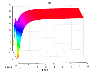
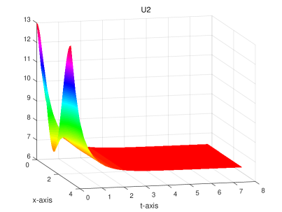
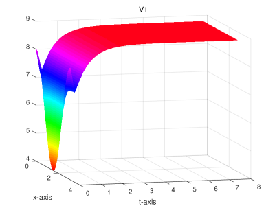
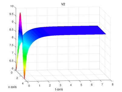
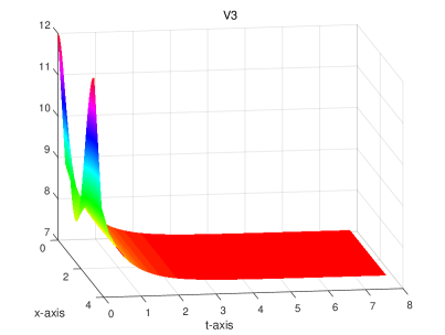
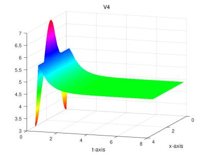
Figure 1: $Q_{4}$ finally dominates with the equilibrium $(13.5757,\ 6.4243,\ 8.7879,\ 8.7879,\ 7.0303,\ 4.3940)$ when $(a_{1},\ a_{2},\ c_{1},\ c_{2},\ c_{3},\ c_{4})=(1,\ 2,\ 3,\ 4,\ 5,\ 6)$

4 Numerical experiments

This section presents some numerical experiments for system (1)-(3). The parameters are set as

$$(a_{1},a_{2},c_{1},c_{2},c_{3},c_{4})=(1,2,3,4,5,6).$$

The considered region is $\Omega=[0,\pi]$. The initial conditions are assumed as

$$\phi_{1}=10-3\cos(2x),\quad\phi_{2}=10+3\cos(2x),$$

$$\psi_{1}=6+2\cos(2x),\quad\psi_{2}=8-2\cos(2x),\quad\psi_{2}=10+2\cos(2x),\quad\psi_{2}=5-2\cos(2x),$$

where $x\in\Omega$. Therefore,

$$M_{0}=\frac{1}{\pi}\int_{0}^{\pi}(\phi_{1}+\phi_{2})=20,\quad N_{0}=\frac{1}{\pi}\int_{0}^{\pi}(\psi_{1}+\psi_{2}+\psi_{3}+\psi_{4})=29,$$

and

$$W_{1}=\frac{1}{\pi}\int_{0}^{\pi}(\psi_{1}+\psi_{2}-\phi_{1})=4,\quad W_{2}=\frac{1}{\pi}\int_{0}^{\pi}(\psi_{3}+\psi_{4}-\phi_{2})=5.$$

By simple calculation, $D_{1}=a_{1}c_{2}(a_{2}+c_{4})+a_{2}c_{3}(a_{1}+c_{1})+c_{2}c_{3}(a_{1}+a_{2})=132$, and condition $(I_{3}^{c})\wedge I_{4}^{c}$ holds because

$$(I_{3}^{c}):a_{2}c_{3}(a_{1}+c_{1})N_{0}=1160\geq 528=D_{1}W_{1},$$

$$(I_{4}^{c}):a_{1}c_{2}(a_{2}+c_{4})N_{0}=928\geq 660=D_{1}W_{2}.$$

According to Lemma 2.2, $Q_{4}$ dominates the system and the equilibrium point is

$$(13.5757,6.4243,8.7879,8.7879,7.0303,4.3940).$$

The numerical solution of system (1)-(3) is illustrated in Figure 1, which is consistent with the uniform convergence result stated in Theorem 1.3.

5 Conclusions

This paper has demonstrated a lower and upper solution method to investigate the asymptotic behaviour of the conservative reaction-diffusion system which is associated with a Markovian process algebra model. In particular, we have proved the uniform convergence of the solution with time to its constant equilibrium for a case study, together with experimental results illustrations. As future work, the techniques and results established in this paper are expected to extend to more general Markov process algebra models. In addition, the relationship among the reaction-diffusions, the fluid approximations and the Markov chains, will be further investigated in the future.