Iterative execution of discrete and inverse discrete Fourier transforms with applications for signal denoising via sparsification

Abstract

We describe a family of iterative algorithms that involve the repeated execution of discrete and inverse discrete Fourier transforms. One interesting member of this family is motivated by the discrete Fourier transform uncertainty principle and involves the application of a sparsification operation to both the time domain and frequency domain data with convergence obtained when time domain sparsity hits a stable pattern. This sparsification variant has practical utility for signal denoising, in particular the recovery of a periodic spike signal in the presence of Gaussian noise. General convergence properties and denoising performance are demonstrated using simulation studies. We are not aware of prior work on such iterative Fourier transformation algorithms and have written this paper in part to solicit feedback from others in the field who may be familiar with similar techniques.

¹Department of Biomedical Data Science
Dartmouth College
Hanover, NH 03755, USA
rob.frost@dartmouth.edu

1 Problem statement

We consider a class of iterative discrete Fourier transform [1] techniques described by Algorithm (1). The structure of this algorithm is broadly motivated by iterative methods such as the alternating direction method of multipliers (ADMM) [2] and expectation-maximization (EM) [3]. The family of algorithms we consider take a real-valued vector $\mathbf{x}\in\mathbb{R}^{n}$ as input and then repeatedly perform the following sequence of actions:

• Execute a function $h():\mathbb{R}^{n}\to\mathbb{R}^{n}$ on $\mathbf{x}$.

• Perform a discrete Fourier transform, $dft()$, on the output of $h()$. The $j^{th}$ element of the complex-valued vector output by the discrete Fourier transform, $dft(\mathbf{x})_{j}$, is defined as:

  $$dft(\mathbf{x})_{j}=\sum_{k=1}^{n}x_{k}e^{-i2\pi jk/n}$$ (1)

• Execute a function $g():\mathbb{C}^{n}\to\mathbb{C}^{n}$ on the complex vector output by the discrete Fourier transform.

• Transform the output of $g()$ back into the real domain via the inverse discrete Fourier transform, $dft^{-1}()$. The $j^{th}$ element of the real-valued vector output by the inverse discrete Fourier transform, $dft^{-1}(\mathbf{c})_{j}$, is defined as:

  $$dft^{-1}(\mathbf{c})_{j}=\frac{1}{n}\sum_{k=1}^{n}c_{k}e^{i2\pi jk/n}$$ (2)

This iteration can expressed as:

$$\mathbf{x}_{k}=\begin{cases}h(\mathbf{x}_{k})\ &k=0\\ h(dft^{-1}(g(dft(\mathbf{x}_{k-1}))))&k\geq 1\\ \end{cases}$$ (3)

Convergence of the algorithm is determined by a function $c()$ that compares $\mathbf{x}_{k}$ to $\mathbf{x}_{k-1}$, i.e., the output of $h()$ on the current iteration to the version from the prior iteration. When convergence is obtained, the output from the last execution of $h()$ is returned. See Algorithm (1) for a detailed definition. For this general family of algorithms, a key question relates to what combinations of $h()$, $g()$, and $c()$ functions and constraints on $\mathbf{x}$ enable convergence. We are specifically interested in scenarios involving convergence to a value that is relevant for a specific data analysis application, e.g., a denoising or optimization problem.

Algorithm 1 Iterative application of discrete Fourier and inverse Fourier transforms

Inputs:

• $\mathbf{x}\in\mathbb{R}^{n}$ $\triangleright$ Input data

• $i_{m}$ $\triangleright$ The maximum number of iterations

Outputs:

• $\mathbf{y}\in\mathbb{R}^{n}$ $\triangleright$ Output data

• $i_{c}$ $\triangleright$ Number of iterations completed

1:$i=1$ $\triangleright$ Initialize iteration index

2:$\mathbf{x}_{0}=\mathbf{x}$ $\triangleright$ Initialize $\mathbf{x}_{i}$

3:while $i\leq i_{m}$ do

4:     $\mathbf{x}^{*}_{i}=h(\mathbf{x}_{i-1})$ $\triangleright$ Apply function $h():\mathbb{R}^{n}\to\mathbb{R}^{n}$ to $\mathbf{x}_{i-1}$

5:     if $c(\mathbf{x}^{*}_{i},\mathbf{x}^{*}_{i-1})$ then $\triangleright$ Check for convergence using indicator function $c()$ with domain $\{\mathbb{R}^{n},\mathbb{R}^{n}\}$

6:         break $\triangleright$ If convergence conditions met, stop the iteration      

7:     $\mathbf{w}_{i}=\textit{dft}(\mathbf{x}^{*}_{i})$ $\triangleright$ Compute discrete Fourier transform of $\mathbf{x}^{*}_{i}$

8:     $\mathbf{w}^{*}_{i}=g(\mathbf{w}_{i})$ $\triangleright$ Apply function $g():\mathbb{C}^{n}\to\mathbb{C}^{n}$ to complex vector $\mathbf{w}_{i}$

9:     $\mathbf{x}_{i}=\textit{dft}^{-1}(\mathbf{w}^{*}_{i})$ $\triangleright$ Compute inverse discrete Fourier transform of $\mathbf{w}^{*}_{i}$

10:     $i=i+1$ $\triangleright$ Increment iteration index return $(\mathbf{x}^{*}_{i},i)$ $\triangleright$ Return the output of the final execution of $h()$

1.1 Trivial cases

If both $h()$ and $g()$ are the identify function, then convergence occurs after a single iteration and the entire algorithm operates as the identify function, i.e., $h(dft^{-1}(g(dft(\mathbf{x})))=dft^{-1}(dft(\mathbf{x}))=\mathbf{x}$. Similarly, if just one of $h()$ or $g()$ is the identify function, then the algorithm simplifies to the repeated execution of the non-identify function, e.g., if $g()$ is the identify function then $h(dft^{-1}(g(dft(\mathbf{x})))=h(dft^{-1}(dft(\mathbf{x})))=h(\mathbf{x})$. In general, we will assume that neither $h()$ nor $g()$ are the identify function and that the number of iterations until convergence, $i_{c}$, is a function of $\mathbf{x}$, i.e., if $\mathbf{x}$ is a random vector, then $i_{c}$ is a random variable.

1.2 Generalizations

A number of generalizations of Algorithm (1) are possible:

1. Matrix-valued input: Instead of accepting a vector $\mathbf{x}\in\mathbb{R}^{n}$ as input, the algorithm could accept a matrix $\mathbf{X}\in\mathbb{R}^{n\times m}$ (or higher-dimensional array) with $\textit{dft}()$ and $\textit{dft}^{-1}()$ replaced by two-dimensional counterparts.

2. Complex-valued input: Instead of just real values, elements of the input could be allowed to take complex or hypercomplex (e.g., quaternion or octonion) values with a correponding change to the complex, or hypercomplex, discrete Fourier transform.

3. Alternative invertable discrete transform: The discrete Fourier transform could be replaced by another invertable discrete transform, e.g., discrete wavelet transform [4]. More broadly, a similar approach could be used with any invertable discrete function.

We will explore the first generalization in this paper but restrict our interest to the real-valued discrete Fourier transform and leave the other generalizations to future work.

2 Related techniques

Algorithm (1) is related to both standard discrete Fourier analysis techniques and iterative algorithms that alternate between dual problem representations. Although a detailed comparison is not possible without defining $h()$, $g()$, and $c()$, some general observations are possible.

2.1 Relationship to standard discrete Fourier analysis

The discrete Fourier transform is widely used in many areas of data analysis with common applications including signal processing [5], image analysis [6], and efficient evaluation of convolutions [7]. The standard structure for these applications is the transformation of real-valued data (e.g, time-valued signal or image) into the frequency domain via a discrete Fourier transform, computation on the frequency domain representation, and final transformation back into the time/location domain via an inverse discrete Fourier transform. For example, to preserve specific frequencies in a signal, the original data can be transformed into the frequency domain via a discrete Fourier transform, the coefficients for non-desired frequencies set to zero, and a filtered time domain signal generated via an inverse transformation. A similar structure is found in the application of other invertable discrete transforms. A key difference between this type of application and the approach discussed in this paper relates to number of executions of the forward and inverse transforms. Specifically, standard discrete Fourier analysis involves just the single application of forward and inverse transforms separated by execution of a single function. In contrast, the method described by Algorithm (1) involves the repeated execution of forward and inverse transforms interleaved by the execution of $h()$ and $g()$ functions until the desired convergence conditions are obtained.

2.2 Relationship to other iterative algorithms

Algorithm (1) shares features with a range of methods (e.g., ADMM [2], Dykstra’s algorithm [8], and EM [3]) that alternate between coupled representations of a problem on each iteration. For ADMM, an optimization problem is solved by alternating between 1) estimating the value of the primal variable that minimizes the Lagrangian with the Lagrangian variables fixed and 2) updating the Lagrangian or dual variables using the most recent primal variable value. Dykstra’s algorithm is also used to solve optimization problems and, for many scenarios, is exactly equivalent to ADMM [9]. For EM, a likelihood maximization problem is solved by alternatively 1) finding the probability distribution of latent variables that maximizes the expected likelihood using fixed parameter values and 2) finding parameter values that maximize the expected likihood given the most recent latent variable distribution. ADMM, Dykstra’s algorithm and EM can all therefore be viewed as techniques that alternatively update different parameter subsets of a common function. In contrast, Algorithm (1) alternates between two different functions, $h()$ and $g()$, that are applied to the same data before and after an invertable discrete transform. Thus, while Algorithm (1) is broadly similar to these techniques, it cannot be directly mapped to these methods. We are not aware of existing iterative algorithms that are equivalent to Algorithm (1).

3 Iterative convergence under sparsification

An interesting subclass of the general iterative method detailed in Algorithm 1 involves the use of sparsification functions for both $h()$ and $g()$ with $c()$ identifying convergence when a stable sparsity pattern is achieved in the output of $h()$. Iterating between time domain and frequency domain sparsification is motivated by the discrete Fourier transform uncertainty principal [10], which constrains the total number of zero values in the time domain data and frequency domain representation generated by a discrete Fourier transform. Attempts to induce sparsity in one domain will reduce sparsity in the other domain with the implication that setting both $h()$ and $g()$ to sparsification functions will not simply result in the generation of a vector of all 0 elements. Instead, for scenarios where the iterative algorithm converages, the solution will represent a stable compromise between time and frequency domain sparsity.

We can explore the general convergence properties of Algorithm 1 using sparsification functions for $h()$ and $g()$ via the following simulation design:

• Set $\mathbf{x}$ to a length $n$ vector of $\mathcal{N}(0,1)$ random variables.

• Define $h()$ to generate a sparse version of $\mathbf{x}$ where the proportion $p$ of elements with the smallest absolute values are set to 0.

• Define $g()$ to generate a sparse version of $\mathbf{w}$ where the proportion $p$ of complex coefficients with the smallest magnitudes are set to $0+0i$.

• Define $c()$ to identify convergence when the indices of 0 values in the output of $h()$ are identical on two sequential iterations.

• The discrete and inverse discrete Fourier transforms are realized using the Fast Fourier Transform.

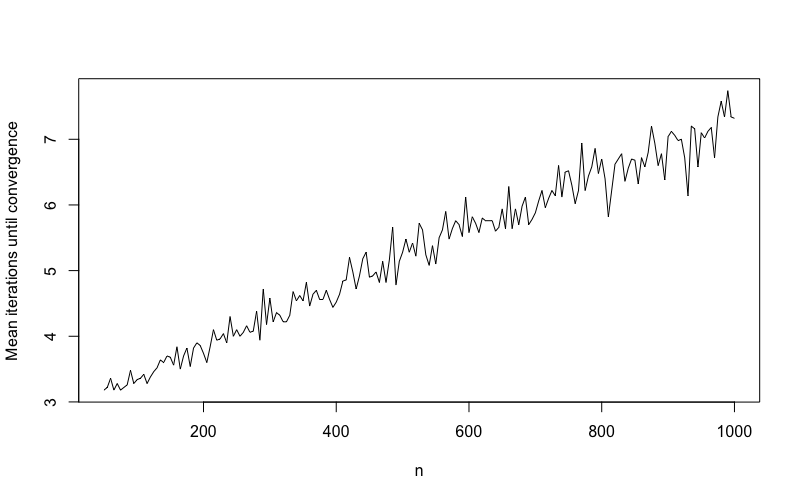
Figure 1: Mean iterations until convergence for random length $n$ vectors of $\mathcal{N}(0,1)$ random variables and $h()$ and $g()$ functions that rank order the elements according to absolute value or magnitude and set the bottom 50% to 0. Convergence is based on repeating the same pattern of sparsity after execution of $h()$ on two sequential iterations.

Following this design, we applied the algorithm to 50 simulated $\mathbf{x}$ vectors for each distinct $n$ value in the range from 50 to 1,000 using the sparse proportion of $p=0.5$ and the maximum number of iterations $i_{m}=50$. Figure 1 below displays the mean number of iterations until convergence as a function of $n$. Figure 2 illustrates the results from a similar simulation that used a fixed $n$ of 500 and sparse proportion value ranging from $0.1$ to $0.9$. For all of the tests visualized in Figures 1 and 2, the algorithm converged to a stable pattern of sparsity in $\mathbf{x}$. Not surprisingly, the number of iterations required to achieve a stable sparsity pattern increased with the growth in either $n$ or $p$. If $h()$ and $g()$ are changed to set all elements with absolute value or magnitude below the mean to 0 (see simulation design in Section 4), the relationship between mean iterations until convergence and $n$ is similar to that shown in Figure 1. Changing the generative model for $\mathbf{x}$ to include a non-random periodic signal (e.g., sinusodial signal or spike signal) also generates similar convergence results.

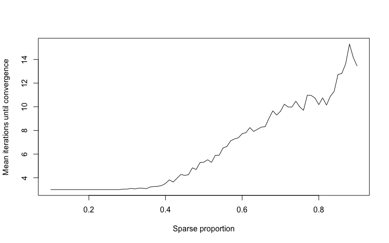
Figure 2: Mean iterations until convergence for random length 500 vectors of $\mathcal{N}(0,1)$ random variables. For these results $h()$, $g()$, and $c()$ have similar definitions as detailed for Figure 1. In this case, $n$ was fixed at 500 and the sparsity proportion varied between 0.1 and 0.9.

4 Detection of spike signals using iterative convergence

To assess the pratical utility of a sparsification version of Algorithm 1 for signal denoising, we used the following simulation design:

• Set $\mathbf{x}$ to the combination of a periodic spike signal $\mathbf{s}$ and Gaussian noise $\boldsymbol{\varepsilon}$, $\mathbf{x}=\mathbf{s}+\boldsymbol{\varepsilon}$, with:

  • Elements $s_{i},i\in(1,...,n)$ of $\mathbf{s}$ set to 0 for all $i\neq a\lambda$ and generated as $U(\alpha_{min},\alpha_{max})$ random variables for $i=a\lambda,a\in(1,...,b)$ where $b$ is the total number of cycles and $\lambda\geq 1$ is the period.

  • Elements $\varepsilon_{i}$ of $\boldsymbol{\varepsilon}$ are generated as independent random variables with distribution $\mathcal{N}(0,\sigma^{2})$.

• Define $h()$ to generate a sparse version of $\mathbf{x}$ where all elements $x_{i}\leq 1/n\sum_{j=1}^{n}|x_{j}|$ are set to 0.

• Define $g()$ to generate a sparse version of $\mathbf{w}$ where all elements $w_{i}\leq 1/n\sum_{j=1}^{n}|w_{j}|$ are set to $0+0i$ (here the $||$ operation represents the magnitude of the complex number $w_{j}$).

• Define $c()$ to identify convergence when the indices of 0 values in the output of $h()$ are identical on two sequential iterations.

Figure 3 shows an example of $\mathbf{x}$ generated according to this simulation model with $\alpha_{min}=\alpha_{max}=2.5,b=16,\lambda=8$ and $\sigma^{2}=0.5$. For this specific example, the method converges in seven iterations and perfectly recovers the periodic spike signal.

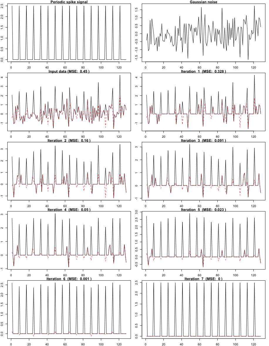
Figure 3: Results from the application of Algorithm 1 to an $\mathbf{x}$ vector simulated according to the model detailed in Section 4 with $\alpha_{min}=2.5,\alpha_{max}=2.5,b=16,\lambda=8$ and $\sigma^{2}=0.5$. The top panels show the periodic spike signal and Gaussian noise. The remaining panels show the input data and output from the $h()$ sparsification function after each iteration of the algorithm with the error relative to the spike signal captured as a dashed red line and quantified via the mean squared error.

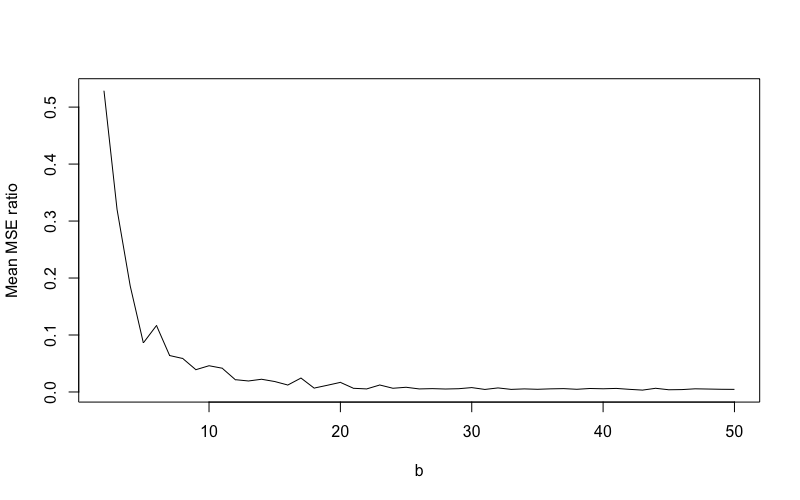
Figure 4: Average mean squared error (MSE) ratio relative to the number of cycles, b, captured in the input $\mathbf{x}$ vector. The MSE ratio is computed as $MSE_{c}/MSE_{1}$ where $MSE_{c}$ represents the MSE after convergence and $MSE_{1}$ represents the MSE after the first execution of $h()$ on the input $\mathbf{x}$.

To more broadly charaterize signal recovery for this simulation design, multiple $\mathbf{x}$ vectors were generated for different values of $\alpha_{min},\alpha_{max},b,\lambda$, and $\sigma^{2}$. Figure 4 shows the relationship between the MSE ratio achieved on converge averaged across 50 simulated $\mathbf{x}$ vectors and the number of cycles, $b$, captured in $\mathbf{x}$. The MSE ratio is specifically computed as $MSE_{c}/MSE_{1}$ where $MSE_{c}$ is the mean squared error (MSE) between the output of the method after convergence and the spike signal $\mathbf{s}$ and $MSE_{1}$ is the MSE for the output from the first execution of $h()$. For this simulation design, the average MSE ratio is very close to 0 for $b\geq 20$, which reflects near perfect recovery of the input periodic spike signal. Figure 5 captures the association between the average MSE ratio and the number of iterations completed by the algorithm ($b$ was fixed at 20 for this simulation). These results demonstrate that signal recovery consistently improves on each iteration of the algorithm with the lowest MSE achieved upon convergence. Figure 6 captures the association between the average MSE ratio achieved on convergence and Gaussian noise variance ($b$ was fixed at 20 for this simulation). These results demonstrate the expected increase in signal recovery error with increase noise variance and, importantly, show that the method still achieves improved noise recovery relative to just a single execution of $h()$ at high levels of noise.

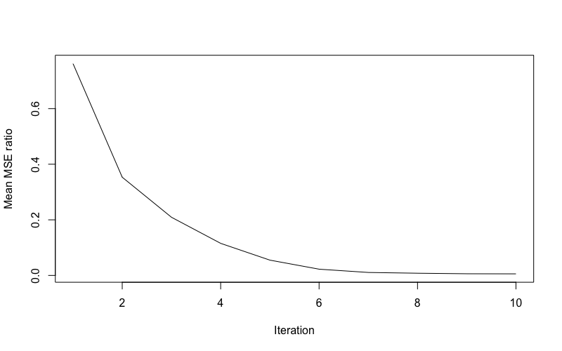
Figure 5: Average MSE ratio after each iteration of the algorithm.

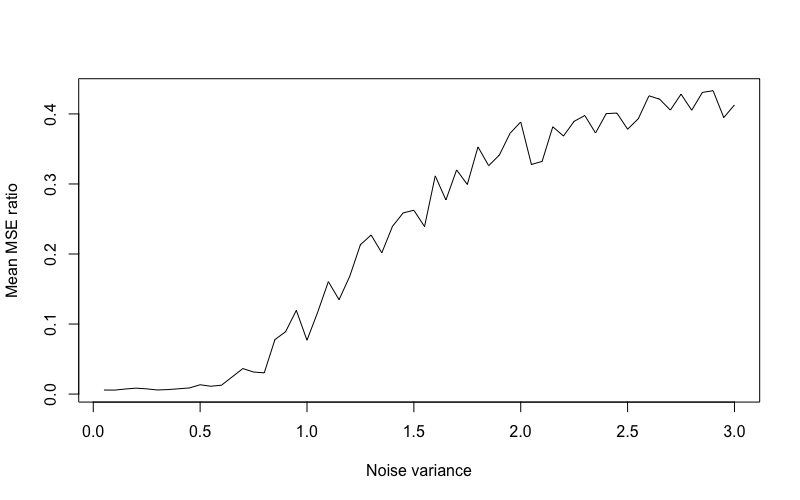
Figure 6: Average mean squared error (MSE) ratio relatieve to the variance of the Gaussian noise, $\sigma^{2}$, added to the periodic spike signal.

To explore the generalization where the input is a matrix rather than a vector, we also tested a simulation model where an input $n\times n$ matrix $\mathbf{X}$ is generated as follows:

• Generate a length $n$ vector $\mathbf{s}$ that contains a periodic spike signal using the logic above.

• Create the signal matrix $\mathbf{S}$ as $\mathbf{S}=\mathbf{s}\mathbf{s}^{T}$.

• Generate an $n\times n$ noise matrix $\mathcal{E}$ whose elements are independent $\mathcal{N}(0,\sigma^{2})$ random variables.

• Create the input $n\times n$ matrix $\mathbf{X}$ as $\mathbf{X}=\mathbf{S}+\mathcal{E}$.

Figure 7 shows an example of $\mathbf{X}$ generated according to this simulation model with $\alpha_{min}=\alpha_{max}=2.5,b=16,\lambda=8$ and $\sigma^{2}=0.5$. For this specific example, the method converges in 24 iterations and perfectly recovers the periodic spike signal matrix. The convergence properties for this type of matrix input when evaluated across multiple simulations mirror those for the vector input shown in Figures 4, 5, and 6.

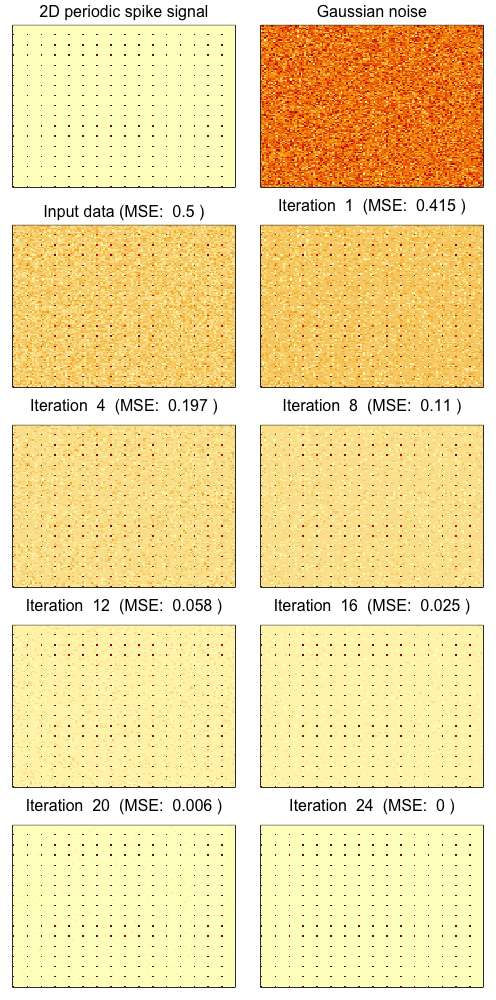
Figure 7: Results from the application of Algorithm 1 to a $\mathbf{X}$ matrix simulated according to the model detailed in Section 4 with $\alpha_{min}=2.5,\alpha_{max}=2.5,b=16,\lambda=8$ and $\sigma^{2}=0.5$. The top panels show the periodic spike signal matrix and Gaussian noise matrix. The remaining panels show the input matrix and output from the $h()$ sparsification function after each iteration with the error relative to the signal matrix quantified via the mean squared error.

5 Next steps

We wrote this short paper to both document the idea and solicit feedback from others in the field regarding any prior work that may been done involving the iterative application of discrete Fourier and inverse discrete Fourier transforms. Areas for future work in this space include:

• Exploring the theoretical basis for the denoising performance shown in Section 4. This will include proving convergence of the algorithm when $h()$ and $g()$ are sparsification functions similar to what is defined in Section 3.

• Performing a comparative evaluation of the sparsification version against other approaches for signal denoising, e.g., basis pursuit [11]. This will include simulation of data according to a broader range of signal and noise patterns.

• Exploring other classes of $h()$, $g()$ and $c()$ functions and associated analysis problems, e.g., soft thresholding.

• Exploring the generalization of the method to complex or hypercomplex-valued inputs.

• Exploring the generalization to other invertable discrete transforms, e.g., discrete wavelet transform [4].

References

- [1] Ronald N Bracewell. The Fourier transform and its applications. McGraw Hill, Boston, 3rd ed edition, 2000.
- [2] Stephen Boyd, Neal Parikh, Eric Chu, Borja Peleato, and Jonathan Eckstein. Distributed optimization and statistical learning via the alternating direction method of multipliers. Found. Trends Mach. Learn., 3(1):1–122, jan 2011.
- [3] A. P. Dempster, N. M. Laird, and D. B. Rubin. Maximum likelihood from incomplete data via the em algorithm. Journal of the Royal Statistical Society. Series B (Methodological), 39(1):1–38, 1977.
- [4] Stphane Mallat. A Wavelet Tour of Signal Processing, Third Edition: The Sparse Way. Academic Press, Inc., USA, 3rd edition, 2008.
- [5] D Sundararajan. Fourier Analysis-A Signal Processing Approach. 1st ed. 2018 edition.
- [6] Ann Maria John, Kiran Khanna, Ritika R Prasad, and Lakshmi G Pillai. A review on application of fourier transform in image restoration. In 2020 Fourth International Conference on I-SMAC (IoT in Social, Mobile, Analytics and Cloud) (I-SMAC), pages 389–397, 2020.
- [7] Lu Chi, Borui Jiang, and Yadong Mu. Fast fourier convolution. In H. Larochelle, M. Ranzato, R. Hadsell, M.F. Balcan, and H. Lin, editors, Advances in Neural Information Processing Systems, volume 33, pages 4479–4488. Curran Associates, Inc., 2020.
- [8] Richard L. Dykstra. An algorithm for restricted least squares regression. Journal of the American Statistical Association, 78(384):837–842, 1983.
- [9] Ryan J. Tibshirani. Dykstra’s algorithm, admm, and coordinate descent: Connections, insights, and extensions. In Proceedings of the 31st International Conference on Neural Information Processing Systems, NIPS’17, pages 517–528, Red Hook, NY, USA, 2017. Curran Associates Inc.
- [10] David L. Donoho and Philip B. Stark. Uncertainty principles and signal recovery. SIAM Journal on Applied Mathematics, 49(3):906–931, 1989.
- [11] Shaobing Chen and D. Donoho. Basis pursuit. In Proceedings of 1994 28th Asilomar Conference on Signals, Systems and Computers, volume 1, pages 41–44 vol.1, 1994.