A Generalized Latent Factor Model Approach to Mixed-data Matrix Completion with Entrywise Consistency

Abstract

Matrix completion is a class of machine learning methods that concerns the prediction of missing entries in a partially observed matrix. This paper studies matrix completion for mixed data, i.e., data involving mixed types of variables (e.g., continuous, binary, ordinal). We formulate it as a low-rank matrix estimation problem under a general family of non-linear factor models and then propose entrywise consistent estimators for estimating the low-rank matrix. Tight probabilistic error bounds are derived for the proposed estimators. The proposed methods are evaluated by simulation studies and real-data applications for collaborative filtering and large-scale educational assessment.

Keywords: Matrix completion, generalized latent factor model, mixed data, entrywise consistency, max norm

1 Introduction

Missing data are commonly encountered when we analyze real-world data, especially for large-scale data involving many observations and variables. Matrix completion refers to a rich family of machine learning methods that concern the prediction of missing entries in a partially observed matrix. Matrix completion methods have received wide applications, such as collaborative filtering (Goldberg et al., 1992; Feuerverger et al., 2012), social network recovery (Jayasumana et al., 2019), sensor localization (Biswas et al., 2006), and educational and psychological measurement (Bergner et al., 2022; Chen et al., 2021).

Many matrix completion methods consider real-valued matrices (Candès and Recht, 2009; Candès and Tao, 2010; Keshavan et al., 2010; Klopp, 2014; Koltchinskii et al., 2011; Negahban and Wainwright, 2012; Chen et al., 2020b; Xia and Yuan, 2021). Their theoretical guarantees are typically established under a linear factor model (e.g. Bartholomew et al., 2008), which says the underlying complete data matrix can be decomposed as the sum of a low-rank signal matrix ${\mathbf{M}}$ and a mean-zero noise matrix. Under this statistical model, the matrix completion task becomes to estimate the signal matrix ${\mathbf{M}}$ based on the observed data entries. However, many real applications of matrix completion involve mixed types of variables (e.g., continuous, count, binary, ordinal), for which the linear factor model may not be suitable. Methods have been developed for matrix completion with specific variable types, such as binary (Cai and Zhou, 2013; Davenport et al., 2014; Han et al., 2020, 2022), categorical (Bhaskar, 2016; Klopp et al., 2015), count (Cao and Xie, 2015; McRae and Davenport, 2021; Robin et al., 2019), and mixed data (Robin et al., 2020). Non-linear factor models, which are extensions of the linear factor model, are typically assumed in these works.

A matrix completion method is typically evaluated by a mean squared error (MSE) $\sum_{i=1}^{n}\sum_{j=1}^{p}(\widehat{m}_{ij}-m_{ij}^{*})^{2}/(np)$, where $n\times p$ is the size of the data matrix, and $\widehat{\mathbf{M}}=(\widehat{m}_{ij})_{n\times p}$ and ${\mathbf{M}}^{*}=(m_{ij}^{*})_{n\times p}$ are the estimated and true signal matrices, respectively. Probabilistic error bounds have been established for the MSE in the literature (see Chen et al., 2020b; Chen and Li, 2022; Cai and Zhou, 2016, and references therein). Under suitable conditions, these error bounds imply that the MSE decays to zero when both $n$ and $p$ grow to infinity, which is viewed as a notion of statistical consistency for matrix completion. However, this notion of consistency slightly differs from that in our traditional sense; that is, the MSE converging to zero does not imply the convergence of each individual entry, which, however, may be important in some applications which concern the prediction of individual data entries. Entrywise results for matrix completion have been established under linear factor models (Abbe et al., 2020; Chen et al., 2019, 2020b; Chernozhukov et al., 2021). However, such results are not available for non-linear factor models, and extending these entrywise results to non-linear factor models is non-trivial.

This paper considers mixed-data matrix completion under a generalized latent factor model (GLFM) framework (Bartholomew et al., 2008; Skrondal and Rabe-Hesketh, 2004) which includes many widely used non-linear factor models as special cases. Under this model framework, we propose two methods that ensure entrywise consistency under dense and sparse missingness settings. Both methods apply to an initial estimate whose MSE converges to zero. They refine the initial estimate by solving some estimating equations constructed based on the initial estimate. The difference between the two methods is that one involves data splitting while the other does not. The two methods have the same asymptotic behavior under a dense setting where the proportion of observed entries does not decay to zero. In that case, their entrywise error rate matches the MSE of the initial estimate up to a logarithm factor, suggesting that there is virtually no loss when performing refinement. However, under a sparse setting where the proportion of observed entries converges to zero, the procedure with data splitting achieves a smaller error rate than the one without data splitting, and the error rate of the data splitting procedure matches the MSE of the initial estimate up to a logarithm factor. Our theoretical analysis further shows that a constrained joint maximum likelihood estimator (Chen et al., 2020a) for the GLFM automatically performs a refinement procedure without data splitting, which implies that this estimator is minimax optimal in an entrywise sense under a dense setting and a suitable asymptotic regime. The proposed methods are evaluated by simulation studies and real-data applications to collaborative filtering and large-scale educational assessment.

The rest of the paper is organized as follows. In Section 2, we introduce a generalized latent factor model for matrix completion with mixed data. In Section 3, two methods for achieving entrywise consistency are introduced. Theoretical guarantees on the proposed methods are established in Section 4. Simulation studies and real data examples are given in Sections 5 and 6, respectively. Finally, we conclude with some discussions in Section 7. Additional theoretical results, proofs of the theorems, and additional simulation results are given in the supplementary material.

2 Mixed-data Matrix Completion

2.1 Notation

For a positive integer $n$, let $[n]:=\{1,\cdots,n\}$ be the set containing all the integers 1, …, $n$. We let $\|\mathbf{x}\|$ denote the standard Euclidean norm for a vector $\mathbf{x}=(x_{1},...,x_{n})^{T}$ and $\|\mathbf{x}\|_{\infty}=\max_{i}|x_{i}|$ be the infinity norm (also called the maximum norm) of a vector. For a matrix ${\mathbf{X}}=(x_{ij})_{n\times m}$, let $\|{\mathbf{X}}\|_{F}$, $\|{\mathbf{X}}\|_{*}$ and $\|{\mathbf{X}}\|_{2}$ denote its Frobenius, nuclear and spectral norms, respectively. We use $\|{\mathbf{X}}\|_{\max}:=\max_{i\in[n],j\in[m]}|x_{ij}|$ to denote the matrix maximum norm, and use $\|{\mathbf{X}}\|_{2\to\infty}:=\sup_{\|{\mathbf{u}}\|=1}\|{\mathbf{X}}{\mathbf{u}}\|_{\infty}$ to denote the two-to-infinity norm. According to Proposition 6.1, Cape et al. (2019), the two-to-infinity norm is the same as the maximum matrix row norm $\|{\mathbf{X}}\|_{2\to\infty}=\max_{i\in[n]}(\sum_{j\in[p]}x_{ij}^{2})^{1/2}$. For two sequences of real numbers, we write $a_{n,p}\ll b_{n,p}$ (or $a_{n,p}=o(b_{n,p})$) if $\lim_{n,p\to\infty}a_{n,p}/b_{n,p}=0$, $a_{n,p}\gg b_{n,p}$ if $\lim_{n,p\to\infty}a_{n,p}/b_{n,p}=\infty$, $a_{n,p}\lesssim b_{n,p}$ (or $a_{n,p}=O(b_{n,p}))$ if there is a positive constant $M$ independent with $n$ and $p$, such that $|a_{n,p}|\leq M|b_{n,p}|$, $a_{n,p}\gtrsim b_{n,p}$ if there is a positive constant $c$ independent with $n$ and $p$, such that $|a_{n,p}|\geq c|b_{n,p}|$, and $a_{n,p}\sim b_{n,p}$ if $b_{n,p}\lesssim a_{n,p}\lesssim b_{n,p}$. For two real numbers $x$ and $y$, we denote their maximum and minimum as $x\vee y=\max(x,y)$ and $x\wedge y=\min(x,y)$, respectively. We use the standard $O_{p}(\cdot)$ and $o_{p}(\cdot)$ notation for stochastic boundedness and convergence in probability, respectively. We use “$\circ$” for the matrix Hadamard (entrywise) product.

2.2 Problem Setup

Consider an $n\times p$ data matrix ${\mathbf{Y}}$, with the $(i,j)$th entry denoted by $Y_{ij}$, for $i\in[n]$ and $j\in[p]$. In the rest, we refer to the rows and columns as the observations and variables, respectively. We do not observe the full matrix due to data missingness. The missing pattern is indicated by an $n\times p$ binary matrix ${\boldsymbol{\Omega}}=(\omega_{ij})_{i\in[n],j\in[p]}$, where $\omega_{ij}=1$ if $Y_{ij}$ is observed and $\omega_{ij}=0$ if $Y_{ij}$ is missing. Matrix completion concerns inferring the value of $Y_{ij}$ for the missing entries, i.e., entries with $\omega_{ij}=0$. We consider variables of mixed types, which occurs in many real-world applications; that is, we allow $Y_{ij}$ in different columns to be of mixed types, such as continuous, binary, ordinal, and count variables.

2.3 A Generalized Latent Factor Model Approach

Additional assumptions are needed for matrix completion, as otherwise, the missing entries can take any feasible values. A typical assumption for matrix completion is a low-rank assumption, i.e., ${\mathbf{Y}}={\mathbf{M}}+\mathbf{E},$ where ${\mathbf{M}}$ is a low-rank signal matrix, and $\mathbf{E}$ is the noise matrix whose entries are independent and mean-zero. Let the rank of ${\mathbf{M}}$ be $r$. Then we can write ${\mathbf{Y}}={\boldsymbol{\Theta}}{\mathbf{A}}^{T}+\mathbf{E}$, where ${\boldsymbol{\Theta}}$ and ${\mathbf{A}}$ are $n\times r$ and $p\times r$ matrices, respectively. This model is typically known as a linear factor model (e.g. Bartholomew et al., 2008), where ${\boldsymbol{\Theta}}$ and ${\mathbf{A}}$ are referred to as the factor-score and loading matrices, respectively. The matrix completion task then becomes an estimation problem, i.e., estimating the signal matrix ${\mathbf{M}}={\boldsymbol{\Theta}}{\mathbf{A}}^{T}$ based on the observed data entries.

However, the linear factor model may be restricted when not all variables are continuous. The GLFM is an extension of the linear factor model (Bartholomew et al., 2008; Skrondal and Rabe-Hesketh, 2004). It assumes that entries $Y_{ij}$ are independent, and the probability density function of $Y_{ij}$ (with respect to some baseline measure) takes an exponential family form $f_{j}(y_{ij}|m_{ij},\phi_{j})=\exp\big{[}\phi_{j}^{-1}\big{\{}y_{ij}m_{ij}-b_{j}(m_{ij})\big{\}}+c_{j}(y_{ij},\phi_{j})\big{]},$ where $b_{j}$ and $c_{j}$ are pre-specified functions, $m_{ij}$ is the $(i,j)$th entry of a low-rank signal matrix ${\mathbf{M}}={\boldsymbol{\Theta}}{\mathbf{A}}^{T}$ and $\phi_{j}$ is a dispersion parameter. The density function depends on variable $j$ so that the variables can be of different types. We give some examples below.

• For a continuous variable $j$, we may assume $f_{j}$ to be a normal density function, where $\phi_{j}$ is the variance, $b_{j}(m_{ij})=m_{ij}^{2}/2$ and $c_{j}(y_{ij},\phi_{j})=-y_{ij}^{2}/(2\phi_{j})-(\log(2\pi\phi_{j}))/2$. When all the variables follow this normal model, the data matrix follows a linear factor model.

• Consider a binary or ordinal variable $j$ such that $Y_{ij}$ in $\{0,1,...,k_{j}\}$ for some given $k_{j}\geq 1$, where $k_{j}=1$ and $k_{j}>1$ correspond to binary and ordinal variables, respectively. We can assume $f_{j}$ to follow a Binomial logistic model, for which $\phi_{j}=1$, $b_{j}(m_{ij})=k_{j}\log(1+\exp(m_{ij}))$ and $c_{j}(y_{ij},\phi_{j})=\log(k_{j}!)-\log(y_{ij}!)-\log((k_{j}-y_{ij})!)$. This model has been considered in Masters and Wright (1984) with psychometric applications. When all the variables are binary and follow this logistic model, the data matrix is said to follow a multidimensional two-parameter logistic (M2PL) item response theory model (Reckase, 2009). This model has been considered in Davenport et al. (2014) for the completion of binary matrices.

• A Poisson model may be assumed for count variables $j$, for which $\phi_{j}=1$, $b_{j}(m_{ij})=\exp(m_{ij})$ and $c_{j}(y_{ij},\phi_{j})=-\log(y_{ij}!)$. When all the variables follow this Poisson model, the joint model for the data matrix is known as a Poisson factor model (Wedel et al., 2003). This Poisson model has been considered in Robin et al. (2019) and Robin et al. (2020) for count data with missing values.

Under the GLFM, ${\mathbb{E}}{\mathbf{Y}}=(b^{\prime}_{j}(m_{ij}))_{n\times p}$, where $b^{\prime}_{j}(\cdot)$ denotes the derivative of the known function $b_{j}(\cdot)$. Thus, matrix completion under the GLFM again boils down to estimating the signal matrix ${\mathbf{M}}={\boldsymbol{\Theta}}{\mathbf{A}}^{T}$. This estimation problem will be investigated in the rest. We note that a similar GLFM framework has been considered in Robin et al. (2020) for analyzing mixed data with missing values. However, they focused on evaluating the estimation accuracy by the MSE, while our main focus is the entrywise loss.

3 Refined Estimation for Entrywise Consistency

As pointed out in the Introduction, the accuracy in estimating ${\mathbf{M}}$ is typically measured by the MSE, or equivalently, a scaled Frobenius norm $\|\widehat{\mathbf{M}}-{\mathbf{M}}^{*}\|_{F}/\sqrt{np}$, where ${\mathbf{M}}^{*}$ is the underlying true signal matrix. We say an estimator is F-consistent, if $\|\widehat{\mathbf{M}}-{\mathbf{M}}^{*}\|_{F}/\sqrt{np}=o_{p}(1)$. As discussed in Section 3.3 below, a few F-consistent estimators are available under general or specific GLFMs. However, the F-consistency only guarantees consistency in an average sense – the proportion of inconsistently estimated entries decays to zero. It cannot guarantee entrywise consistency, i.e., the consistency of $\widehat{m}_{ij}$ for each individual data entry, which may be important in some applications concerning the prediction of individual data entries. Entrywise results for matrix completion, which focus on the loss $\|\widehat{\mathbf{M}}-{\mathbf{M}}^{*}\|_{\max}$, have been established under linear factor models (Abbe et al., 2020; Chen et al., 2019, 2020b; Chernozhukov et al., 2021) but not under the GLFM. Establishing entrywise consistency is more challenging under the GLFM due to the involvement of non-linear link functions of the exponential family. In what follows, we propose methods that can improve an F-consistent estimator to an entrywise consistent (E-consistent) estimator under the GLFM.

3.1 Refinement without Data Splitting

Let $\widehat{{\mathbf{M}}}$ be given by an F-consistent estimator based on observed data $({\mathbf{Y}}\circ{\boldsymbol{\Omega}},{\boldsymbol{\Omega}})$; see Section 3.3 for examples of such estimators. We propose the following refinement procedure that inputs $\widehat{\mathbf{M}}$ and outputs an E-consistent estimator.

Method 1 (Refinement Procedure without Data Splitting).

• Input: Observed data $({\mathbf{Y}}\circ{\boldsymbol{\Omega}},{\boldsymbol{\Omega}})$, an initial estimate $\widehat{\mathbf{M}}$ and a pre-specified constant $C_{2}$.

• Step 1. Perform singular value decomposition (SVD) to $\widehat{{\mathbf{M}}}$ and obtain $\widehat{{\mathbf{V}}}_{r}\in\mathbb{R}^{p\times r}$ which contains the top-$r$ right singular vectors of $\widehat{{\mathbf{M}}}$.

• Step 2. Calculate $\widehat{{\mathbf{A}}}=\textbf{proj}_{\{{\mathbf{A}}\in\mathbb{R}^{p\times r}:\|{\mathbf{A}}\|_{2\to\infty}\leq C_{2}\}}(\widehat{{\mathbf{V}}}_{r})$, where $\textbf{proj}_{\{{\mathbf{A}}\in\mathbb{R}^{p\times r}:\|{\mathbf{A}}\|_{2\to\infty}\leq C_{2}\}}(\cdot)$ denotes a projection operator that projects a $p\times r$ matrix to satisfy the two-to-infinity norm constraint.

• Step 3. For each $i\in[n]$, calculate $\widetilde{{\boldsymbol{\theta}}}_{i}$ by solving an equation:

  $$\sum_{j=1}^{p}\omega_{ij}\{y_{ij}-b^{\prime}_{j}((\widehat{{\mathbf{a}}}_{j})^{T}\widetilde{{\boldsymbol{\theta}}}_{i})\}\widehat{{\mathbf{a}}}_{j}=\mathbf{0}_{r}.$$ (1)

• Step 4. For each $j\in[p]$, obtain $\widetilde{{\mathbf{a}}}_{j}$ by solving the following equation:

  $$\sum_{i=1}^{n}\omega_{ij}\{y_{ij}-b^{\prime}_{j}((\widetilde{{\mathbf{a}}}_{j})^{T}\widetilde{{\boldsymbol{\theta}}}_{i})\}\widetilde{{\boldsymbol{\theta}}}_{i}=\mathbf{0}_{r}.$$ (2)

• Output: $\widetilde{{\mathbf{M}}}=\widetilde{{\boldsymbol{\Theta}}}(\widetilde{{\mathbf{A}}})^{T}$, where $\widetilde{{\boldsymbol{\Theta}}}=(\widetilde{{\boldsymbol{\theta}}}_{1},\cdots,\widetilde{{\boldsymbol{\theta}}}_{n})^{T}\in\mathbb{R}^{n\times r}$ and $\widetilde{{\mathbf{A}}}=(\widetilde{{\mathbf{a}}}_{1},\cdots,\widetilde{{\mathbf{a}}}_{p})^{T}\in\mathbb{R}^{p\times r}$ are obtained from Steps 3 and 4, respectively.

We comment on the implementation. First, the constant $C_{2}$ depends on the true signal matrix ${\mathbf{M}}^{*}$. Recall that we assume ${\mathbf{M}}^{*}$ to be of rank $r$ under the GLFM. Thus, ${\mathbf{M}}^{*}$ can be decomposed as ${\mathbf{M}}^{*}={\mathbf{U}}^{*}_{r}{\mathbf{D}}^{*}_{r}({\mathbf{V}}^{*}_{r})^{T}$, where ${\mathbf{U}}_{r}^{*}\in\mathbb{R}^{n\times r}$ and ${\mathbf{V}}_{r}^{*}\in\mathbb{R}^{p\times r}$ are the left and right singular matrices corresponding to the non-zero singular values, and ${\mathbf{D}}_{r}^{*}\in\mathbb{R}^{r\times r}$ is a diagonal matrix whose diagonal elements are the singular values $\sigma_{1}({\mathbf{M}}^{*})\geq\cdots\geq\sigma_{r}({\mathbf{M}}^{*})>0$. We require $C_{2}$ to satisfy $C_{2}\geq\|{\mathbf{V}}_{r}^{*}\|_{2\to\infty}$. On the other hand, $C_{2}$ should not be chosen too large. As will be shown in Section 4.2, it is assumed that $C_{2}$ has the same asymptotic order as $\|{\mathbf{V}}_{r}^{*}\|_{2\to\infty}$; otherwise, the error bound for $\|\widetilde{\mathbf{M}}-{\mathbf{M}}^{*}\|_{\max}$ needs additional modification. Second, we note that the projection in Step 2 is very easy to perform. Let ${\mathbf{V}}=(\mathbf{v}_{1},...,\mathbf{v}_{p})^{T}$ be a $p\times r$ matrix. Then $\textbf{proj}_{\{{\mathbf{A}}\in\mathbb{R}^{p\times r}:\|{\mathbf{A}}\|_{2\to\infty}\leq C_{2}\}}({\mathbf{V}})=(\widetilde{\mathbf{v}}_{1},...,\widetilde{\mathbf{v}}_{p})^{T}$, where $\widetilde{\mathbf{v}}_{i}=\mathbf{v}_{i}$ if $\|\mathbf{v}_{i}\|\leq C_{2}$ and $\widetilde{\mathbf{v}}_{i}=(C_{2}/\|\mathbf{v}_{i}\|)\mathbf{v}_{i}$ otherwise. Finally, we provide a remark on solving the equations in Steps 3 and 4.

Remark 1.

In Steps 3 and 4, we propose to solve some estimating equations. As will be shown in Section 4, these equations have a unique solution with probability converging to $1$ under a suitable asymptotic regime. These steps are equivalent to performing optimization to certain log-likelihood functions. Let $\ell({\mathbf{M}})=\sum_{i,j:\omega_{ij}=1}\big{\{}y_{ij}m_{ij}-b_{j}(m_{ij})\big{\}}$ be a weighted log-likelihood function based on observed data $({\mathbf{Y}}\circ{\boldsymbol{\Omega}},{\boldsymbol{\Omega}})$, where the individual log-likelihood terms are weighted by the dispersion parameters. Then, solving the estimating equations (1) is equivalent to solving $\widetilde{{\boldsymbol{\Theta}}}\in\operatornamewithlimits{arg\,max}_{{\boldsymbol{\Theta}}}\ell({\boldsymbol{\Theta}}\widehat{{\mathbf{A}}}^{T})$, and solving the estimating equations (2) is equivalent to solving $\widetilde{{\mathbf{A}}}\in\operatornamewithlimits{arg\,max}_{{\mathbf{A}}}\ell(\widetilde{{\boldsymbol{\Theta}}}{{\mathbf{A}}}^{T})$. This is due to that the estimating equations (1) and (2) are obtained by taking the partial derivatives of $\ell({{\boldsymbol{\Theta}}}{{\mathbf{A}}}^{T})$with respect to ${\boldsymbol{\Theta}}$ and ${\mathbf{A}}$, respectively, and that the objective function $\ell({{\boldsymbol{\Theta}}}{{\mathbf{A}}}^{T})$ is convex with respect to ${\boldsymbol{\Theta}}$ and ${\mathbf{A}}$ given the other.

We provide an informal theorem under a simplified setting to shed some light on the asymptotic behavior of Method 1. Its formal version is Theorem 3 in Section 4.2, which is established under a more general setting.

Theorem 1 (An informal and simplified version of Theorem 3).

Assume that $\lim_{n,p\to\infty}{\mathbb{P}}(\|\widehat{{\mathbf{M}}}-{\mathbf{M}}^{*}\|_{F}\leq e_{M,F})=1$ and let $\widetilde{{\mathbf{M}}}$ be obtained by Method 1. Then, under suitable assumptions on ${\mathbf{M}}^{*}$ and the asymptotic regime $\pi_{\min}=\pi_{\max}=\pi$, $r$ is fixed, $p\pi,n\pi\gg(\log(np))^{3}$, and $\{(n\wedge p)\pi\}^{-1/2}\lesssim(np)^{-1/2}e_{M,F}\ll\pi^{1/2}(\log(np))^{-2}$, we have $\|\widetilde{{\mathbf{M}}}-{\mathbf{M}}^{*}\|_{\max}\lesssim(\log(np))^{2}\cdot\pi^{-1/2}(np)^{-1/2}e_{{\mathbf{M}},F}.$

We consider the asymptotic regime $\{(n\wedge p)\pi\}^{-1/2}\lesssim(np)^{-1/2}e_{M,F}$ above because $\{(n\wedge p)\pi\}^{-1/2}$ is the minimax error rate of $(np)^{-1/2}\|\widehat{{\mathbf{M}}}-{\mathbf{M}}^{*}\|_{F}$; see Chen and Li (2022).

3.2 Refinement with Data Splitting

From Theorem 1 above, we see that $\|\widetilde{\mathbf{M}}-{\mathbf{M}}^{*}\|_{\max}$ achieves the same error rate as $\|\widehat{\mathbf{M}}-{\mathbf{M}}^{*}\|_{F}/\sqrt{np}$ (up to a logarithm factor) when $\pi\sim 1$. However, when $\pi=o(1)$, the rate of $\|\widetilde{\mathbf{M}}-{\mathbf{M}}^{*}\|_{\max}$ becomes worse than that of $\|\widehat{\mathbf{M}}-{\mathbf{M}}^{*}\|_{F}/\sqrt{np}$, due to the factor $\pi^{-1/2}$ in the upper bound. This term comes from the worst case scenario when $\widehat{{\mathbf{A}}}-{\mathbf{A}}^{*}$ is highly dependent with $(\omega_{ij})_{j\in[p]}$ for some $i$ (e.g., $\widehat{{\mathbf{a}}}_{j}-{\mathbf{a}}_{j}^{*}\approx\omega_{ij}\mathbf{b}$ for all $j\in[p]$, some $i\in[n]$, and some random vector $\mathbf{b}\in\mathbb{R}^{r}$). To obtain a better error rate under the max norm, we propose a new procedure that uses a data splitting step to break the dependence between $\widehat{{\mathbf{A}}}$ and ${\boldsymbol{\Omega}}$. The proposed data splitting method is similar to the one proposed in Chernozhukov et al. (2021) for linear factor models, where a similar dependence issue exists. However, due to the non-linear link functions involved in the GLFM, the development of our method and its theory faces unique challenges.

Let ${\mathcal{N}}_{1}\subset[n]$ be a random subset independent of $({\mathbf{Y}},{\boldsymbol{\Omega}})$. In particular, we let $I(i\in{\mathcal{N}}_{1})$ be i.i.d. Bernoulli random variables with ${\mathbb{P}}(i\in{\mathcal{N}}_{1})=1/2$ for $i\in[n]$, where $I(\cdot)$ denotes the indicator function. By the law of large numbers, ${\mathcal{N}}_{1}$ is a subset of $[n]$ with size around $n/2$. We further let ${\mathcal{N}}_{2}=[n]\setminus{\mathcal{N}}_{1}$.

Method 2 (Refinement Procedure with Data Splitting).

• Input: Observed data $({\mathbf{Y}}\circ{\boldsymbol{\Omega}},{\boldsymbol{\Omega}})$, a constraint parameter $C_{2}$, and initial estimates $\widehat{{\mathbf{M}}}_{{\mathcal{N}}_{k},\cdot}$ for ${\mathbf{M}}_{{\mathcal{N}}_{k},\cdot}=(m_{ij})_{i\in{\mathcal{N}}_{k},j\in[p]}$ obtained based on $({\mathbf{Y}}\circ{\boldsymbol{\Omega}},{\boldsymbol{\Omega}})_{{\mathcal{N}}_{k},\cdot}=(y_{ij}\omega_{ij},\omega_{ij})_{i\in{\mathcal{N}}_{k},j\in[p]}$ for $k=1,2$.

• Step 1. Perform SVD to $\widehat{{\mathbf{M}}}_{{\mathcal{N}}_{1},\cdot}$ and calculate $\widehat{{\mathbf{V}}}_{r}^{(1)}\in\mathbb{R}^{p\times r}$ which contains the top-$r$ right singular vectors of $\widehat{{\mathbf{M}}}_{{\mathcal{N}}_{1},\cdot}$.

• Step 2. Calculate $\widehat{{\mathbf{A}}}^{(1)}=(\widehat{{\mathbf{a}}}_{j}^{(1)})_{j\in[p]}^{T}=\textbf{proj}_{\{{\mathbf{A}}\in\mathbb{R}^{p\times r}:\|{\mathbf{A}}\|_{2\to\infty}\leq C_{2}\}}(\widehat{{\mathbf{V}}}_{r}^{(1)})$.

• Step 3. Calculate $\widetilde{{\boldsymbol{\Theta}}}_{{\mathcal{N}}_{2}}=(\widetilde{{\boldsymbol{\theta}}}_{i})^{T}_{i\in{\mathcal{N}}_{2}}$, where for each $i\in{\mathcal{N}}_{2}$, $\widetilde{{\boldsymbol{\theta}}}_{i}$ is obtained by solving the equation $\sum_{j=1}^{p}\omega_{ij}\{y_{ij}-b_{j}^{\prime}((\widehat{{\mathbf{a}}}_{j}^{(1)})^{T}\widetilde{{\boldsymbol{\theta}}}_{i})\}\widehat{{\mathbf{a}}}_{j}^{(1)}=\mathbf{0}_{r}.$

• Step 4. Calculate $\widetilde{{\mathbf{A}}}^{(1)}=(\widetilde{{\mathbf{a}}}_{j}^{(1)})^{T}_{j\in[p]}$, where for each $j\in[p]$, $\widetilde{{\mathbf{a}}}_{j}^{(1)}$ is obtained by solving the equation $\sum_{i\in{\mathcal{N}}_{2}}\omega_{ij}\{y_{ij}-b_{j}^{\prime}((\widetilde{{\mathbf{a}}}_{j}^{(1)})^{T}\widetilde{{\boldsymbol{\theta}}}_{i})\}\widetilde{{\boldsymbol{\theta}}}_{i}=0_{r}.$

• Step 5. Swap ${\mathcal{N}}_{1}$ and ${\mathcal{N}}_{2}$ in Steps 1–4, and obtain $\widetilde{{\boldsymbol{\Theta}}}_{{\mathcal{N}}_{1}}$ and $\widetilde{{\mathbf{A}}}^{(2)}$ accordingly.

• Output: $\widetilde{{\mathbf{M}}}=(\widetilde{m}_{ij})_{i\in[n],j\in[p]}$, where $(\widetilde{m}_{ij})_{i\in{\mathcal{N}}_{1},j\in[p]}=\widetilde{{\boldsymbol{\Theta}}}_{{\mathcal{N}}_{1}}(\widetilde{{\mathbf{A}}}^{(2)})^{T}$ and $(\widetilde{m}_{ij})_{i\in{\mathcal{N}}_{2},j\in[p]}=\widetilde{{\boldsymbol{\Theta}}}_{{\mathcal{N}}_{2}}(\widetilde{{\mathbf{A}}}^{(1)})^{T}$.

The comments on Method 1 regarding the choice of $C_{2}$, the projection operator, and the solutions to the estimating equations apply similarly to Method 2. As the rows and columns of the data matrix play a similar role, the above method can be modified to split the columns instead of the rows. As summarized in Theorem 2, which is an informal and simplified version of Theorem 4 in Section 4.3, Method 2 improves the error rate of Method 1. In fact, $\|\widetilde{\mathbf{M}}-{\mathbf{M}}^{*}\|_{\max}$ now achieves the same error rate as $\|\widehat{\mathbf{M}}-{\mathbf{M}}^{*}\|_{F}/\sqrt{np}$ up to a logarithm factor, regardless of the missing rate $\pi$.

Theorem 2 (An informal and simplified version of Theorem 4).

Assume that $\lim_{n,p\to\infty}{\mathbb{P}}(\|\widehat{{\mathbf{M}}}_{{\mathcal{N}}_{k}\cdot}-{\mathbf{M}}^{*}_{{\mathcal{N}}_{k}\cdot}\|_{F}\leq e_{{\mathbf{M}},F})=1$ for $e_{{\mathbf{M}},F}$ $(k=1,2)$ and $\widetilde{{\mathbf{M}}}$ is obtained by Method 2. Then, under suitable assumptions on ${\mathbf{M}}^{*}$ and the asymptotic regime $\pi_{\min}=\pi_{\max}=\pi$, $r$ is fixed, $p\pi,n\pi\gg(\log(np))^{3}$, and $\{(n\wedge p)\pi\}^{-1/2}\lesssim(np)^{-1/2}e_{M,F}\ll(\log(np))^{-2}$, we have $\|\widetilde{{\mathbf{M}}}-{\mathbf{M}}^{*}\|_{\max}\lesssim(\log(np))^{2}(np)^{-1/2}e_{{\mathbf{M}},F}.$

As the data splitting in Method 2 is random, it may be beneficial to run it multiple times and then aggregate the resulting estimates. We describe this variation of Method 2 below. For a fixed number of random splittings, the asymptotic behavior of Method 2’ is the same as that of Method 2.

• • Input: Observed data $({\mathbf{Y}}\circ{\boldsymbol{\Omega}},{\boldsymbol{\Omega}})$ a constraint $C_{2}$ and the number of data splittings tot.

  • Step 1. Independently generate index sets ${\mathcal{N}}_{1}^{(k)}and{\mathcal{N}}_{2}^{(k)}$ and obtain initial estimates $\widehat{\mathbf{M}}_{{\mathcal{N}}_{1}}^{(k)}$ and $\widehat{\mathbf{M}}_{{\mathcal{N}}_{2}}^{(k)}$ based on $({\mathbf{Y}}\circ{\boldsymbol{\Omega}},{\boldsymbol{\Omega}})_{{\mathcal{N}}_{1}^{(k)},\cdot}=(y_{ij}\omega_{ij},\omega_{ij})_{i\in{\mathcal{N}}_{1}^{(k)},j\in[p]}$ and $({\mathbf{Y}}\circ{\boldsymbol{\Omega}},{\boldsymbol{\Omega}})_{{\mathcal{N}}_{2}^{(k)},\cdot}=(y_{ij}\omega_{ij},\omega_{ij})_{i\in{\mathcal{N}}_{2}^{(k)},j\in[p]}$, respectively, for $k=1,2,...,\mbox{tot}$.

  • Step 2. For $k=1,...,\mbox{tot}$, run Method 2 with data $({\mathbf{Y}}\circ{\boldsymbol{\Omega}},{\boldsymbol{\Omega}})$, initial estimates $\widehat{\mathbf{M}}_{{\mathcal{N}}_{1}}^{(k)}$ and $\widehat{\mathbf{M}}_{{\mathcal{N}}_{2}}^{(k)}$, index sets ${\mathcal{N}}_{1}^{(k)},{\mathcal{N}}_{2}^{(k)}$ and a constraint parameter $C_{2}$. Obtain outputs $\widetilde{\mathbf{M}}^{(k)}$, $k=1,...,\mbox{tot}$.

  • Output: $\widetilde{{\mathbf{M}}}=(\sum_{k=1}^{\text{tot}}\widetilde{\mathbf{M}}^{(k)})/\mbox{tot}$ .

3.3 F-consistent Estimators

Our refinement methods require input from an F-consistent estimator. We give examples of F-consistent estimators.

The constrained joint maximum likelihood estimator (CJMLE) solves the following optimization problem

$$(\widehat{\boldsymbol{\Theta}},\widehat{\mathbf{A}})\in\arg\max_{{\boldsymbol{\Theta}},{\mathbf{A}}} ~{}~{}\ell({\boldsymbol{\Theta}}{\mathbf{A}}^{T}),~{}~{}\mbox{s.t.} ~{}{\boldsymbol{\Theta}}\in\mathbb{R}^{n\times r},{\mathbf{A}}\in\mathbb{R}^{p\times r},\|{\boldsymbol{\Theta}}\|_{2\to\infty}\leq C,\|{\mathbf{A}}\|_{2\to\infty}\leq C.$$ (3)

The estimate of ${\mathbf{M}}$ is then given by $\widehat{\mathbf{M}}=\widehat{\boldsymbol{\Theta}}\widehat{\mathbf{A}}^{T}$. The terminology “joint likelihood” comes from the latent variable model literature (Chapter 6, Skrondal and Rabe-Hesketh, 2004). This literature distinguishes the joint likelihood from the marginal likelihood, depending on whether entries of ${\boldsymbol{\Theta}}$ are treated as fixed parameters or random variables, where the marginal likelihood is more commonly adopted in the statistical inference of traditional latent variable models. This estimator was first proposed in Chen et al. (2020a) for the estimation of high-dimensional GLFM, and an error bound on $\|\widehat{\mathbf{M}}-{\mathbf{M}}^{*}\|_{F}$ under a general matrix completion setting can be found in Theorem 2 of Chen and Li (2022).

More specifically, suppose that the true signal matrix has a decomposition ${\mathbf{M}}^{*}={\boldsymbol{\Theta}}^{*}({\mathbf{A}}^{*})^{T}$, such that $\|{\boldsymbol{\Theta}}^{*}\|_{2\to\infty}\leq C$ and $\|{\mathbf{A}}^{*}\|_{2\to\infty}\leq C.$ Then, under a similar setting as in Theorems 1 and 2, we have $\lim_{n,p\to\infty}{\mathbb{P}}(\|\widehat{{\mathbf{M}}}-{\mathbf{M}}^{*}\|_{F}/\sqrt{np}\leq\kappa^{\dagger}\{(p\wedge n)\pi\}^{-1/2})=1$, for some finite positive constant $\kappa^{\dagger}$. As shown in Proposition 1 of Chen and Li (2022), $\{(p\wedge n)\pi\}^{-1/2}$ is also the minimax lower bound for estimating ${\mathbf{M}}$ in the scaled Frobenius norm, which is why this lower bound is assumed for $(np)^{-1/2}e_{{\mathbf{M}},F}$ in Theorems 1 and 2.

We note that $(\widehat{\boldsymbol{\Theta}},\widehat{\mathbf{A}})$ given by the CJMLE jointly maximizes the weighted likelihood. Following the discussion in Remark 1 on the connection between the estimating equations and the weighted likelihood, $\widehat{\mathbf{M}}=\widehat{\boldsymbol{\Theta}}\widehat{\mathbf{A}}^{T}$ will remain unchanged when input into Method 1 if $C_{2}$ is chosen properly according to $C$. Consequently, the CJMLE is automatically entrywise consistent under a suitable asymptotic regime; see Remark 3 for a discussion.

• The CJMLE requires solving a non-convex optimization problem for which convergence to the global optimum is not always guaranteed. The nuclear-norm-based estimator (NBE) is a convex approximation to CJMLE. It solves the following optimization problem

  $$\widehat{\mathbf{M}}\in\arg\max_{{\mathbf{M}}} ~{}~{}\ell({\mathbf{M}}),~{}~{}\mbox{s.t.}~{}~{}\|{\mathbf{M}}\|_{\max}\leq\rho^{\prime},\|{\mathbf{M}}\|_{*}\leq\rho^{\prime}\sqrt{rnp}.$$ (4)

  The nuclear norm constraint is introduced, since $\{{\mathbf{M}}\in\mathbb{R}^{n\times p}:\|{\mathbf{M}}\|_{\max}\leq\rho^{\prime},\|{\mathbf{M}}\|_{*}\leq\rho^{\prime}\sqrt{rnp}\}$ is a convex relaxation of $\{{\mathbf{M}}\in\mathbb{R}^{n\times p}:\|{\mathbf{M}}\|_{\max}\leq\rho^{\prime},\mbox{rank}({\mathbf{M}})\leq r\}$. This estimator has been considered in Davenport et al. (2014) for the completion of binary matrices. When the true model follows the M2PL model and the true signal matrix ${\mathbf{M}}^{*}$ satisfies $\|{\mathbf{M}}^{*}\|_{\max}\leq\rho^{\prime}$, then Theorem 1 of Davenport et al. (2014) implies that under the same setting of Theorems 1 and 2, $\lim_{n,p\to\infty}{\mathbb{P}}(\|\widehat{{\mathbf{M}}}-{\mathbf{M}}^{*}\|_{F}/\sqrt{np}\leq\kappa^{\ddagger}\{(p\wedge n)\pi\}^{-1/4})=1$, where $\kappa^{\ddagger}$ is a finite positive constant which depends on the true model parameters. We believe that the same rate holds for other GLFMs under the simplified setting of Theorems 1 and 2.

• Note that other F-consistent estimators may be available for GLFMs, such as SVD-based methods (Chatterjee, 2015; Zhang et al., 2020), regularized estimators (Klopp, 2014; Koltchinskii et al., 2011; Negahban and Wainwright, 2012; Robin et al., 2020), and methods based on a matrix factorization norm (Cai and Zhou, 2013, 2016).

4 Theoretical Results

4.1 Assumptions and useful quantities

We make the following Assumptions 1 and 2 throughout Section 4.

Assumption 1.

$b_{1}(x)=\cdots=b_{p}(x)=b(x)$ for all $x\in\mathbb{R}$. In addition, $b(x)<\infty$ and $b^{\prime\prime}(x)>0$ for all $x\in\mathbb{R}$.

We note that this assumption is made for ease of presentation. It can be relaxed to allowing functions $b_{j}$ to be variable-specific, and similar theoretical results hold following a similar proof. For each $\alpha>0$, define functions $\kappa_{2}(\alpha)=\sup_{|x|\leq\alpha}b^{\prime\prime}(x),\kappa_{3}(\alpha)=\sup_{|x|\leq\alpha}|b^{(3)}(x)|,\text{ and }\delta_{2}(\alpha)=\inf_{|x|\leq\alpha}b^{\prime\prime}(x).$ Let ${\mathbf{M}}^{*}$ have the SVD ${\mathbf{M}}^{*}={\mathbf{U}}^{*}_{r}{\mathbf{D}}^{*}_{r}({\mathbf{V}}^{*}_{r})^{T}$ where $r$ is the rank of ${\mathbf{M}}^{*}$, ${\mathbf{U}}_{r}^{*}\in\mathbb{R}^{n\times r}$ and ${\mathbf{V}}_{r}^{*}\in\mathbb{R}^{p\times r}$ are the left and right singular matrices corresponding to the top-$r$ singular values, respectively, and ${\mathbf{D}}_{r}^{*}\in\mathbb{R}^{r\times r}$ is a diagonal matrix whose diagonal elements are the singular values $\sigma_{1}({\mathbf{M}}^{*})\geq\cdots\geq\sigma_{r}({\mathbf{M}}^{*})>0$. In order to apply the proposed methods, we need to input $C_{2}$.

Assumption 2.

We choose $C_{2}$ such that $C_{2}\geq\|{\mathbf{V}}_{r}^{*}\|_{2\to\infty}$.

Define the following quantities that depend on ${\mathbf{M}}^{*}$. Let $\rho=\max_{i\in[n],j\in[p]}|m_{ij}^{*}|,C_{1}=\{\|{\mathbf{U}}_{r}^{*}\|_{2\to\infty}\vee(r/n)^{1/2}\}\cdot\sigma_{1}({\mathbf{M}}^{*})$, $\kappa_{2}^{*}=\kappa_{2}(2\rho+1),\delta_{2}^{*}=\delta_{2}(2\rho+1),\text{ and }\kappa_{3}^{*}=\kappa_{3}(6C_{1}C_{2}).$ For the missing pattern ${\boldsymbol{\Omega}}=(\omega_{ij})_{i\in[n],j\in[p]}$, let $\pi_{ij}={\mathbb{P}}(\omega_{ij}=1)$ be the sampling probabilities and $\pi_{\min}=\min_{i\in[n],j\in[p]}\pi_{ij}$ and $\pi_{\max}=\max_{i\in[n],j\in[p]}\pi_{ij}$ be the minimal and maximal sampling probability, respectively.

4.2 Error analysis without data splitting

Theorem 3.

Assume that $\lim_{n,p\to\infty}{\mathbb{P}}(\|\widehat{{\mathbf{M}}}-{\mathbf{M}}^{*}\|_{F}\leq e_{{\mathbf{M}},F})=1$, $\widetilde{{\mathbf{M}}}$ is obtained by Method 1, and the following asymptotic regime holds:

1. $\phi_{1}=\cdots=\phi_{p}=\phi\sim 1$;

2. $\pi_{\min}\sim\pi_{\max}\sim\pi$;

3. $\|{\mathbf{U}}_{r}^{*}\|_{2\to\infty}\lesssim(r/n)^{1/2}$, $\|{\mathbf{V}}_{r}^{*}\|_{2\to\infty}\lesssim(r/p)^{1/2}$, $C_{2}\sim(r/p)^{1/2}$;

4. $\sigma_{r}({\mathbf{M}}^{*})\sim\sigma_{1}({\mathbf{M}}^{*})\sim(np)^{1/2}r^{\eta}$ for some constants $\eta\geq-1$;

5. $p\pi\gg(\kappa_{2}^{*})^{4}(\delta_{2}^{*})^{-6}(\log(np))^{3}\max\Big{[}r^{(1+2\eta)\vee 5},(\kappa_{3}^{*})^{2}r^{(3+4\eta)\vee 7}\Big{]}$;

6. $n\pi\gg(\kappa_{2}^{*})^{2}(\delta_{2}^{*})^{-4}(\log(np))^{2}\max\big{\{}r^{3},(\kappa_{3}^{*})^{2}r^{5}\big{\}}$;

7. $(np)^{-1/2}e_{{\mathbf{M}},F}\ll(\kappa_{2}^{*})^{-2}(\delta_{2}^{*})^{3}(\log(np))^{-2}\min\big{[}r^{-5/2},(\kappa_{3}^{*})^{-1}r^{-7/2}\big{]}\pi^{1/2}.$

Then, with probability converging to $1$, estimating equations in steps 3 and 4 of Method 1 have a unique solution and

$$\begin{split}\|\widetilde{{\mathbf{M}}}-{\mathbf{M}}^{*}\|_{\max}\lesssim(\delta_{2}^{*})^{-2}(\kappa_{2}^{*})^{2}(\log(np))^{2}r^{5/2}\Big{[}\{(n\wedge p)\pi\}^{-1/2}+(np\pi)^{-1/2}e_{{\mathbf{M}},F}\Big{]}.\end{split}$$ (5)

In particular, if we further assume that $r\sim 1$, then, the asymptotic regime requirements R5 – R7 can be simplified as $p\pi\gg(\log(np))^{3}$, $n\pi\gg(\log(np))^{2}$ and $(np)^{-1/2}e_{{\mathbf{M}},F}\ll(\log(np))^{-2}\pi^{1/2}$, and we have that with probability converging to $1$, $\|\widetilde{{\mathbf{M}}}-{\mathbf{M}}^{*}\|_{\max}\lesssim(\log(np))^{2}\big{[}\{(n\wedge p)\pi\}^{-1/2}+(np\pi)^{-1/2}e_{{\mathbf{M}},F}\big{]}.$

Remark 2.

We comment on the asymptotic requirement R1–R7. R1 requires the dispersion parameters to be the same for different $j\in[p]$. This assumption is made for ease of presentation, and it can be easily relaxed to allow varying values of dispersion parameters. It further requires that the dispersion parameter is bounded as $n$ and $p$ grow large. R2 requires $\pi_{\max}$ and $\pi_{\min}$ to be of the same asymptotic order. That is, the missing pattern is not too far from the commonly adopted uniform missingness assumption where all the $\pi_{ij}$ are the same (see, e.g. Candès and Tao, 2010; Davenport et al., 2014). R3 is a standard incoherent condition that is commonly assumed for matrix completion to avoid spiky low-rank matrices (Candès and Recht, 2009; Jain et al., 2013). R4 requires that the non-zero singular values of ${\mathbf{M}}^{*}$ are in the same asymptotic order. In addition, we restrict the analysis to the case where $\eta\geq-1$, because otherwise $\|{\mathbf{M}}^{*}\|_{\max}\ll 1$ and the asymptotic regime is less interesting. We note that R4 can be relaxed to a more general asymptotic regime allowing $\sigma_{r}({\mathbf{M}}^{*})$ and $\sigma_{1}({\mathbf{M}}^{*})$ to have different asymptotic order, and we provide the error analysis under a more general setting in the supplementary material. R5 and R6 require the expected number of non-missing observations for each row and column to be large enough. R7 requires the initial F-consistent estimator to have a sufficiently small estimation error in scaled Frobenius norm. In Corollaries 1 – 3 below, we give sufficient conditions for R5 – R7 under the three specific GLFMs described in Section 2.

Remark 3.

Let $\widehat{{\mathbf{M}}}_{\text{CJMLE}}$ and $\widehat{{\mathbf{M}}}_{NBE}$ denote the constrained joint maximum likelihood estimator and nuclear-norm-based estimator described in Section 3.3, respectively. Also let $\widetilde{{\mathbf{M}}}_{\text{CJMLE}}$ and $\widetilde{{\mathbf{M}}}_{NBE}$ be the corresponding refined estimators by applying Method 1. Theorem 3 indicates that with high probability $\|\widetilde{{\mathbf{M}}}_{\text{CJMLE}}-{\mathbf{M}}^{*}\|_{\max}\lesssim(\log(np))^{2}\pi^{-1}(n\wedge p)^{-1/2}$ and $\|\widetilde{{\mathbf{M}}}_{\text{NBE}}-{\mathbf{M}}^{*}\|_{\max}\lesssim(\log(np))^{2}\pi^{-3/4}(n\wedge p)^{-1/4}$ when $r$ is bounded, under suitable regularity conditions. Note that $\widetilde{{\mathbf{M}}}_{\text{CJMLE}}$ is a fixed point of Method 1 with high probability. Thus, $\widehat{{\mathbf{M}}}_{\text{CJMLE}}=\widetilde{{\mathbf{M}}}_{\text{CJMLE}}$, which implies that we have the same error rate for the estimator $\widehat{{\mathbf{M}}}_{\text{CJMLE}}$ without refinement. Because $\widehat{{\mathbf{M}}}_{\text{CJMLE}}$ is asymptotically minimax when $\pi\sim 1$ in Frobenius norm, we also have $\widehat{{\mathbf{M}}}_{\text{CJMLE}}$ is asymptotically minimax in the matrix max norm.

In the following corollaries, we provide sufficient conditions for R5 - R7 under specific GLFMs discussed earlier.

Corollary 1 (Binomial Model).

Assume that $\lim_{n,p\to\infty}{\mathbb{P}}(\|\widehat{{\mathbf{M}}}-{\mathbf{M}}^{*}\|_{F}\leq e_{{\mathbf{M}},F})=1$ for some non-random $e_{{\mathbf{M}},F}$. In addition, assume that data follow a binomial factor model and that asymptotic requirements R2 - R4 in Theorem 3 hold as $n,p\to\infty$. Then, (5) holds if there is a constant $\epsilon_{0}>0$ such that the following asymptotic regime holds:

1. $p\pi\gg(n\vee p)^{\epsilon_{0}}r^{(3+4\eta)\vee 7}$;

2. $n\pi\gg(n\vee p)^{\epsilon_{0}}r^{5}$;

3. $(np)^{-1/2}e_{{\mathbf{M}},F}\ll(n\wedge p)^{-\epsilon_{0}}\pi^{1/2}r^{-7/2}$;

4. $k_{1}=\cdots=k_{p}=k\sim 1$;

5. $\rho\lesssim\log(n\wedge p)^{1-\epsilon_{0}}$.

In the above corollary, R1 automatically holds because the dispersion parameter $\phi_{j}=1$ in the binomial model.

Corollary 2 (Normal Model).

Assume that $\lim_{n,p\to\infty}{\mathbb{P}}(\|\widehat{{\mathbf{M}}}-{\mathbf{M}}^{*}\|_{F}\leq e_{{\mathbf{M}},F})=1$ for some non-random $e_{{\mathbf{M}},F}$. In addition, assume that data follow a normal factor model and that asymptotic requirements R1 - R4 in Theorem 3 hold as $n,p\to\infty$. Then, (5) holds under the following asymptotic regime:

1. $p\pi\gg(\log(np))^{3}r^{(1+2\eta)\vee 5}$;

2. $n\pi\gg(\log(np))^{2}r^{3}$;

3. $(np)^{-1/2}e_{{\mathbf{M}},F}\ll(\log(np))^{-2}\pi^{1/2}r^{-5/2}.$

Corollary 3 (Poisson Model).

Assume that $\lim_{n,p\to\infty}{\mathbb{P}}(\|\widehat{{\mathbf{M}}}-{\mathbf{M}}^{*}\|_{F}\leq e_{{\mathbf{M}},F})=1$ for some non-random $e_{{\mathbf{M}},F}$. In addition, assume that data follow a Poisson factor model and that asymptotic requirements R2 - R4 in Theorem 3 and R5B –R7B in Corollary 4 hold as $n,p\to\infty$. Then, (5) holds if there is a constant $\epsilon_{0}>0$ such that the following asymptotic regime holds:

1. $r^{1+\eta}\lesssim(\log(n\wedge p))^{1-\epsilon_{0}}$.

Remark 4.

We comment on the asymptotic requirements in the above corollaries. R5B, R6B, R5N and R6N require that rank $r$ is relatively small comparing with $(n\wedge p)\pi$, and it can grow at most of the order $\{(n\wedge p)\pi\}^{\nu_{1}}$ for some constant $\nu_{1}\in(0,1)$. Conditions R5B and R6B are slightly stronger than R5N and R6N, because $\kappa_{3}^{*}=0$ for the normal model while $\kappa_{3}^{*}\sim 1$ for the binomial model. Conditions R7B and R7N require the scaled Frobenius norm of the initial estimator to be small. Many F-consistent estimators, including CJMLE and NBE, have the error rate $(np)^{-1/2}e_{{\mathbf{M}},F}\sim((n\wedge p)\pi)^{-\nu_{2}}$ for some $\nu_{2}\in(0,1)$. For these estimators, R7B and R7N require that $r\lesssim((n\wedge p)\pi)^{\nu_{3}}\pi^{1/2}$ for some $\nu_{3}\in(0,1)$. Condition R8B requires the $k_{j}$s to be the same for different $j\in[p]$ and are bounded. This condition can be easily relaxed to a more general setting with varying but bounded $k_{j}$s. Condition R9B requires that $\rho$ grows much slower than $n$ and $p$. Similar assumptions are made for 1-bit matrix completion (Davenport et al., 2014; Cai and Zhou, 2013). For Poisson factor models, R10P can be achieved either by an arbitrary $r$ with $\eta=-1$ or by $r\lesssim(\log(n\wedge p))^{(1-\epsilon_{0})/(1+\eta)}$ with $\eta>-1$.

4.3 Error analysis with data splitting

Theorem 4.

Assume that $\lim_{n,p\to\infty}{\mathbb{P}}(\|\widehat{{\mathbf{M}}}_{{\mathcal{N}}_{k}\cdot}-{\mathbf{M}}^{*}_{{\mathcal{N}}_{k}\cdot}\|_{F}\leq e_{{\mathbf{M}},F})=1$ for some non-random $e_{{\mathbf{M}},F}$ $(k=1,2)$, and $\widetilde{{\mathbf{M}}}$ is obtained by Method 2. Assume asymptotic requirements R1 - R6 in Theorem 3 hold as $n,p\to\infty$. Also, assume the following asymptotic requirements:

1. $(np)^{-1/2}e_{{\mathbf{M}},F}\ll(\kappa_{2}^{*})^{-2}(\delta_{2}^{*})^{3}(\log(np))^{-2}\min\big{[}r^{-5/2},(\kappa_{3}^{*})^{-1}r^{-7/2}\big{]}.$

Then, with probability converging to $1$, estimating equations in steps 3 and 4 of Method 2 have a unique solution and

$$\begin{split}\|\widetilde{{\mathbf{M}}}-{\mathbf{M}}^{*}\|_{\max}\lesssim(\delta_{2}^{*})^{-2}(\kappa_{2}^{*})^{2}\log^{2}(np)r^{5/2}\Big{[}\{(p\wedge n)\pi\}^{-1/2}+(np)^{-1/2}e_{{\mathbf{M}},F}\Big{]}.\end{split}$$ (6)

In particular, if we further assume that $r\sim 1$, then, the asymptotic regime requirements R5, R6, and R7’ can be simplified as $p\pi\gg(\log(np))^{3}$, $n\pi\gg(\log(np))^{2}$ and $(np)^{-1/2}e_{{\mathbf{M}},F}\ll(\log(np))^{-2}$, and we have that with probability converging to $1$, $\|\widetilde{{\mathbf{M}}}-{\mathbf{M}}^{*}\|_{\max}\lesssim(\log(np))^{2}\big{[}\{(n\wedge p)\pi\}^{-1/2}+(np)^{-1/2}e_{{\mathbf{M}},F}\big{]}.$

Remark 5.

There are two main differences between Theorem 3 and Theorem 4. First, the asymptotic requirement R7 has an extra factor $\pi^{1/2}$ when compared with R7’. Second, the error rate (5) has an extra ${\pi}^{-1/2}$ factor when compared with (6). Thus, when $\pi\ll 1$, Method 1 requires stronger regularity conditions and has a larger error rate. Additional results under a more general asymptotic regime are provided in the supplementary material.

The following corollaries give sufficient conditions for R7’ to hold under specific GLFMs.

Corollary 4 (Binomial Model).

Assume that $\lim_{n,p\to\infty}{\mathbb{P}}(\|\widehat{{\mathbf{M}}}_{{\mathcal{N}}_{k}\cdot}^{(k)}-{\mathbf{M}}^{*}_{{\mathcal{N}}_{k}\cdot}\|_{F}\leq e_{{\mathbf{M}},F})=1$ for some non-random $e_{{\mathbf{M}},F}$ $(k=1,2)$. In addition, assume that data follow a binomial factor model and that asymptotic requirements R2 - R4 in Theorem 3 and R5B, R6B, R8B, R9B in Corollary 1 hold as $n,p\to\infty$. Then, (6) holds if there is a constant $\epsilon_{0}>0$ such that the following asymptotic regime holds:

1. $(np)^{-1/2}e_{{\mathbf{M}},F}\ll(n\wedge p)^{-\epsilon_{0}}r^{-7/2}.$

Corollary 5 (Normal Model).

Assume that $\lim_{n,p\to\infty}{\mathbb{P}}(\|\widehat{{\mathbf{M}}}_{{\mathcal{N}}_{k}\cdot}^{(k)}-{\mathbf{M}}^{*}_{{\mathcal{N}}_{k}\cdot}\|_{F}\leq e_{{\mathbf{M}},F})=1$ for some non-random $e_{{\mathbf{M}},F}$ $(k=1,2)$. In addition, assume that data follow a normal factor model and that asymptotic requirements R1 - R4 in Theorem 3 and R5N, R6N in Corollary 2 hold as $n,p\to\infty$. Then, (6) holds under the following asymptotic regime:

1. $(np)^{-1/2}e_{{\mathbf{M}},F}\ll(\log(np))^{-2}r^{-5/2}.$

Corollary 6 (Poisson Model).

Assume that $\lim_{n,p\to\infty}{\mathbb{P}}(\|\widehat{{\mathbf{M}}}_{{\mathcal{N}}_{k}\cdot}^{(k)}-{\mathbf{M}}^{*}_{{\mathcal{N}}_{k}\cdot}\|_{F}\leq e_{{\mathbf{M}},F})=1$ for some non-random $e_{{\mathbf{M}},F}$ $(k=1,2)$. In addition, assume that data follow a Poisson factor model and that asymptotic requirements R2 - R4 in Theorem 3, R5B, R6B in Corollary 1 ,R7’B in Corollary 4, and R10P in Corollary 3 hold as $n,p\to\infty$. Then, (6) holds.

Remark 4 still applies to Corollary 4 – Corollary 6, except that now we have a better rate when $\pi$ is close to zero.

5 Simulation Study

We evaluate the proposed methods via a simulation study. Eight estimation procedures are considered as listed in Table 1. These procedures are applied under 24 simulation settings, where $n$, $p$, $r$, $\pi_{\max}=\pi_{\min}=\pi$, and variable types are varied. Settings 1-6 are listed in Table 2. The rest of the settings and additional details on data generation can be found in the supplementary material. For each simulation setting, 100 simulations are conducted.

Procedure	Initial estimator	Refinement method	Procedure	Initial estimator	Refinement method
1	NBE		5	CJMLE
2	NBE	Method 1	6	CJMLE	Method 1
3	NBE	Method 2	7	CJMLE	Method 2
4	NBE	Method 2’ (5 runs)	8	CJMLE	Method 2’ (5 runs)

Table 1: Estimation procedures compared in a simulation study.

Setting	$n$	$p$	$r$	$\pi$	Variable Types	Setting	$n$	$p$	$r$	$\pi$	Variable Type
1	400	200	3	0.6	O	4	400	200	3	0.2	O
2	800	400	3	0.6	O	5	800	400	3	0.2	O
3	1600	800	3	0.6	O	6	1600	800	3	0.2	O

Table 2: Simulation settings. ‘Variable type = O’ indicates all the variables are ordinal (with $k_{j}=5$), for which the Binomial model is assumed.

The procedures are evaluated under two loss functions, the scaled Frobenius norm $\|\widehat{\mathbf{M}}-{\mathbf{M}}^{*}\|_{F}/\sqrt{np}$ and the max norm $\|\widehat{\mathbf{M}}-{\mathbf{M}}^{*}\|_{\max}$. The results for Settings 1-6 are given in Figures 1 and 2, and those for the other settings show similar patterns and are given in the supplementary material. First, for each procedure and given $r$ and $\pi$, both the scaled Frobenius norm and the max norm decay as $n$ and $p$ grow simultaneously. Second, comparing the two figures, we see that the error rates are larger under Settings 4-6 than those under Settings 1-3 given the same $n,p$, and $r$, as the proportion of missing entries is higher under Settings 4-6. Third, Procedure 1 (i.e., NBE with no refinement) has larger error rates than its refined versions (Procedures 2-4), suggesting that the refinement procedures reduce the error of the initial NBE. Fourth, we see that Procedures 5 and 6 perform similarly, which is expected as they are asymptotically equivalent, as discussed in Remark 3. Fifth, comparing Procedures 2 and 6, we see that the refined NBE and the refined CJMLE have very similar performance. Similar patterns are observed when comparing Procedures 3 and 7 and when comparing Procedures 4 and 8. At first glance, it may seem a little counter-intuitive. According to Theorems 3 and 4, the error in the max norm of a refined estimator is upper bounded by the error in the scaled Frobenius norm of its initial estimator, and thus, we would expect the CJMLE-based refinements to have smaller errors in the max norm than the NBE-based refinements. The pattern under the current settings may be explained by the SVD steps in Methods 1, 2, and 2’ that project the initial estimate to the space of rank-$r$ matrices. Under these settings, the initial NBE after projection tends to approximate the CJMLE. We note that this is not always the case under other settings. Under settings 23 and 24 (see their results in the supplementary material), the CJMLE tends to outperform the projected NBE, and thus, the CJMLE-based refinements tend to outperform the NBE-based refinements. Finally, comparing within Procedures 2-4 and comparing within Procedures 6-8, we see that Method 1 leads to better empirical performance regardless of the value of $\pi$, even though Method 2 has a faster theoretical convergence speed when $\pi$ approaches 0. We conjecture that for CJMLE and NBE, the resulting $\widehat{\mathbf{A}}$ in Step 2 of Method 1 does not have a high dependence with any rows of ${\boldsymbol{\Omega}}$ when $\omega_{ij}$s are uniformly sampled, and thus, the upper bound in (5) may be improved in this case. We also observe that Method 2’ outperforms Method 2 through aggregating results from multiple runs of Method 2. By running Method 2 five times, Method 2’ has a similar performance as Method 1.

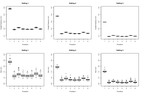
Figure 1: Results from Simulation Settings 1-3. The panels on the first row show the results based on the scaled Frobenius norm, and those on the second row show the results based on the max norm. In each panel, the box plots show the results of the eight procedures in Table 1, each constructed from 100 independent simulations.

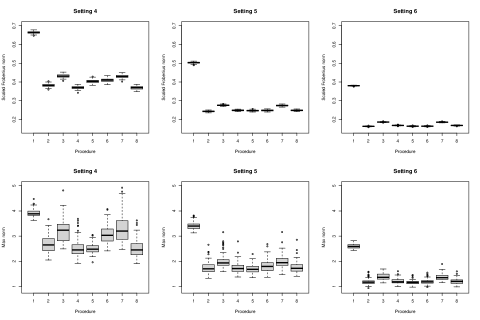
Figure 2: Results from Simulation Settings 4-6. The plots can be interpreted similarly as those in Figure 1.

6 Real Data Examples

6.1 Collaborative Filtering

We apply the proposed method to a MovieLens dataset for movie recommendation (Harper and Konstan, 2015). The dataset contains 943 users’ ratings on 1,682 movies. Only 6.3% of the data entries are observed. For each movie, the raw ratings take integer values from 1 to 5. We transform the values from 0 to 4, and then apply the binomial factor model with $k_{j}=4$ for all $j$. The goal is to predict the unobserved entries for movie recommendations.

Rank	1	2	3	4	5	6	7	8
1	-48928	-49247	-49397	-49253	-49256	-49266	-49266	-49163
2	-53201	-49505	-49767	-48875	-48437	-48493	-48654	-48341
3	-56091	-49284	-49754	-48570	-49022	-49217	-48837	-48207
4	-56235	-49633	-50037	-48611	-51192	-51986	-49174	-48271

Table 3: Test-set log-likelihoods for the MovieLens data. The eight procedures are listed in Table 1.

The eight procedures in Table 1 are considered, with candidate rank $r=1,2,3$, and 4. To evaluate the procedures, we split the data into training and test datasets, where the training and test sets contain 80% and 20% of the observed entries, respectively. We estimate the ${\mathbf{M}}$ matrix using the training set and then evaluate the prediction accuracy by the test-set log-likelihood at the estimated ${\mathbf{M}}$. A larger log-likelihood function value implies a higher prediction accuracy. The results are given in Table 3. The refinement methods improve the test-set log-likelihood of the NBE when $r=2,3,4$ but not when $r=1$, likely due to the rank-one model being too restrictive for the current data. Turning to the results from the CJMLE and its refinements, we see that Procedures 5 and 6 tend to perform similarly, likely due to the asymptotic equivalence between the CJMLE and its refinement by Method 1. We also see that Procedure 8, which is a refinement of CJMLE by Method 2’, tends to improve the test-set log-likelihood of CJMLE under all values of $r$. Procedure 7 also performs fine, despite its relatively high variance brought by performing data splitting only once in Method 2. The good performance of Procedures 7 and 8 is likely due to that the distribution of the data missingness indicators $\omega_{ij}$ is far from a uniform distribution. Instead, their distribution likely depends on the true signal matrix (i.e., people may be more likely to have watched movies that they like), which may lead to dependence between the initial estimate $\widehat{\mathbf{A}}$ and some rows of ${\boldsymbol{\Omega}}$ when data splitting is not performed. Such dependence leads to a larger estimation error. The largest test-set log-likelihood is given by Procedure 8 (i.e., CJMLE refined by Method 2’) when $r=3$.

6.2 Large-scale Assessment in Education

We apply the proposed method to data from the 2018 Program for International Student Assessment (PISA; OECD, 2019a), a large-scale international educational survey operated by the Organization for Economic Co-operation and Development (OECD). We consider a subset of the PISA 2018 dataset, containing 9,970 students’ responses to 415 assessment items. The students were from 37 OECD countries. The 415 assessment items measure four knowledge domains, including mathematics, science, reading, and global competence. A matrix sampling design is adopted in PISA 2018, under which each student was only assigned a subset of assessment items. Consequently, only 15.5% of the entries are observed in the dataset. Under this matrix sampling design, it is not sensible to directly compare students’ performance based on their total scores, as the students answered different assessment items, and the items measure different knowledge domains and are not equally difficult. Among these items, 396 items are dichotomously scored, and 19 items have score levels $0,1$ and $2$. The goal is to predict students’ performance on the items they did not receive in order to compare the performance based on the entire set of items.

We apply the binomial factor model. Similar to the above analysis, we split 80% and 20% of the data into training and test sets and evaluate the prediction accuracy by the test-set log-likelihood. The eight procedures in Table 1 are considered, with candidate rank $r=1,2,3,$ and 4. The results are given in Table 4. First, the refinement methods tend to improve the test-set log-likelihood given by the NBE, except for the case when $r=1$. The results given by the CJMLE and its refinement by Method 1 are similar under all values of $r$. They tend to be better than the refinements given by Methods 2 and 2’, likely due to that the variance brought by data splitting is high in this analysis. Second, the largest test-set log-likelihood is achieved by the CJMLE when the rank $r=2$. The test-set log-likelihoods of the CJMLE and its refinement by Method 1 are similar when $r=2$, and they tend to substantially outperform the rest. In the analysis of PISA data, each of the knowledge domains is believed to correspond to at least one latent factor. Thus, four- or higher-dimensional factor models are typically adopted to jointly model the item responses (see Chapter 9, page 22, OECD, 2019b). Our results suggest that a lower-dimensional factor model may have better prediction performance, though not necessarily have better performance in terms of statistical inference and interpretation. This finding is closely related to the discussion in psychometrics regarding the value of subscores (Haberman, 2008).

Rank	1	2	3	4	5	6	7	8
1	-67205	-67938	-67958	-67921	-67587	-67516	-68204	-68140
2	-71620	-68556	-68733	-67749	-63250	-63313	-64914	-64842
3	-75816	-70092	-70067	-69151	-65476	-65370	-68611	-67693
4	-77632	-72365	-72238	-71640	-72320	-72648	-79466	-75989

Table 4: Test-set log-likelihoods for the PISA data. The eight procedures are listed in Table 1.

7 Discussions

This paper concerns matrix completion for mixed data under a GLFM framework. It proposes entrywise consistent methods for estimating GLFMs based on a partially observed data matrix. Probabilistic error bounds are established for the matrix max norm under sensible asymptotic regimes (see Section 4), and they are extended under a more general asymptotic regime in the supplementary material. These error bounds imply the entrywise consistency and further characterize the asymptotic behaviors of the proposed methods. With these error bounds, optimal results are established under suitable asymptotic regimes. A simulation study shows that for the refined estimators, the error in matrix max norm decays towards zero as $n$ and $p$ grow simultaneously. It also shows that the performance of the NBE can be substantially improved by running the proposed refinement procedures. In contrast, the CJMLE can hardly be improved as it is already equivalent to a refined estimator. The simulation results further suggest that Method 2’ can improve the accuracy of Method 2 by running this data-splitting procedure multiple times and aggregating the results. However, although a smaller upper bound is proven for the error rates of Methods 2 and 2’ when the missing rate is close to 1, these procedures do not outperform Method 1 - the refinement procedure without data splitting - under our simulation settings. This phenomenon is likely due to that the probability of the worst-case scenario occurring for Method 1 is close to zero under the current simulation settings, in which case the upper bound in (5) may be improved. The proposed procedures are applied to two real data examples, one on movie recommendation and the other on large-scale educational assessment. For the movie recommendation example, the best predictive model is a rank-three model obtained by refining the CJMLE with Method 2’. For the educational assessment example, a rank-two model given by the CJMLE turns out to be the most predictive one.

The current work can be extended in several directions. First, some popular factor models, such as the probit model for binary data considered in Davenport et al. (2014), are not exponential family GLFMs. We believe that our refinement procedures and their theory can be extended to many other models beyond exponential family GLFM. This is because the theoretical properties of these procedures mainly rely on the convexity of the loss function with respect to ${\mathbf{M}}$, which still holds under many other non-linear factor models. Second, the optimal rate for estimating GLFMs is worth future investigation. We currently do not know whether our upper bounds are minimax optimal when the dimension $r$ diverges. Sharp lower bounds need to be developed to answer this question. Future research is also needed to investigate whether the error bound for Method 1 can be improved. If not, further simulation studies are needed to find out settings under which Methods 2 and 2’ outperform Method 1.

Supplement Material for “A Generalized Latent Factor Model Approach to Mixed-data Matrix Completion with Entrywise Consistency”

Appendix A Proof of Theorem 4 and additional theoretical results for Method 2 with data splitting

In this section, we obtain the error bound for $\|\widetilde{{\mathbf{M}}}-{\mathbf{M}}^{*}\|_{\max}\leq\max(\|\widetilde{{\boldsymbol{\Theta}}}_{{\mathcal{N}}_{1}}(\widetilde{{\mathbf{A}}}^{(1)})^{T}-{\mathbf{M}}^{*}_{{\mathcal{N}}_{1}\cdot}\|_{\max},\|\widetilde{{\boldsymbol{\Theta}}}_{{\mathcal{N}}_{2}}(\widetilde{{\mathbf{A}}}^{(2)})^{T}-{\mathbf{M}}^{*}_{{\mathcal{N}}_{2}\cdot}\|_{\max})$. We will provide detailed analysis for $\|\widetilde{{\boldsymbol{\Theta}}}_{{\mathcal{N}}_{1}}(\widetilde{{\mathbf{A}}}^{(1)})^{T}-{\mathbf{M}}^{*}_{{\mathcal{N}}_{1}\cdot}\|_{\max}$. The analysis of $\|\widetilde{{\boldsymbol{\Theta}}}_{{\mathcal{N}}_{2}}(\widetilde{{\mathbf{A}}}^{(2)})^{T}-{\mathbf{M}}^{*}_{{\mathcal{N}}_{2}\cdot}\|_{\max}$ is similar and is thus omitted. For the ease of presentation, we drop the superscript $(1)$ in $\widehat{{\mathbf{A}}}^{(1)}$ when the context is clear. Recall that ${\mathbf{M}}^{*}$ has the SVD ${\mathbf{M}}^{*}={\mathbf{U}}_{r}^{*}{\mathbf{D}}_{r}^{*}({\mathbf{V}}_{r}^{*})^{T}$ where ${\mathbf{U}}_{r}^{*}\in\mathbb{R}^{n\times r}$, ${\mathbf{V}}_{r}^{*}\in\mathbb{R}^{p\times r}$ denote the left and right singular matrices, and ${\mathbf{D}}_{r}^{*}=\text{diag}(\sigma_{1}({\mathbf{M}}^{*}),\cdots,\sigma_{r}({\mathbf{M}}^{*}))$.

The rest of the section is organized as follows. In Section A.1, we obtain an error bound for $\|\widehat{{\mathbf{A}}}-{\mathbf{A}}^{*}\|_{F}$ where ${\mathbf{A}}^{*}={\mathbf{V}}_{r}^{*}\widehat{{\mathbf{P}}}$ for a carefully chosen orthogonal matrix $\widehat{{\mathbf{P}}}$. In Section A.2, we provide non-asymptotic and non-probabilistic bounds for solutions to the non-linear estimation equations used in Step 3 and 4 in the proposed Method 2. In Section A.3, we obtain non-asymptotic probabilistic bounds for terms involved in Section A.2. In Section A.4, we put together results in Sections A.1 – A.3 and obtain asymptotic error bounds for $\|\widetilde{{\boldsymbol{\Theta}}}_{{\mathcal{N}}_{2}}-{\boldsymbol{\Theta}}^{*}\|_{2\to\infty}$ (Lemma 23), $\|\widetilde{{\mathbf{A}}}-{\mathbf{A}}^{*}\|_{2\to\infty}$ (Lemma 24), and $\|\widetilde{{\boldsymbol{\Theta}}}_{{\mathcal{N}}_{1}}(\widetilde{{\mathbf{A}}}^{(1)})^{T}-{\mathbf{M}}^{*}_{{\mathcal{N}}_{1}\cdot}\|_{\max}$ (Lemma 25) where ${\boldsymbol{\Theta}}^{*}={\mathbf{U}}_{r}^{*}{\mathbf{D}}_{r}^{*}\widehat{{\mathbf{P}}}$. Finally, we provide additional theoretical results for Method 2 in Section A.5 and the proof of Theorem 4 in Section A.6.

Throughout the analysis, for real number operators, we calculate multiplication and division before the max and min operators (‘$\vee$’ and $`\wedge^{\prime}$) unless otherwise specified. For example, $u(xy\vee z/w)=u\max(xy,z/w)$ for real numbers $x,y,u,w,z$. For two events $A$ and $B$, we say ‘event $A$ has probability at least $1-\epsilon$ on event $B$’, if ${\mathbb{P}}(A^{c}\cap B)\leq\epsilon$. Note that ${\mathbb{P}}(A)\geq 1-\epsilon-{\mathbb{P}}(B^{c})$ in this case.

A.1 Error Analysis for $\widehat{{\mathbf{A}}}$

In this section, we provide an error bound for $\widehat{{\mathbf{A}}}$ given an error bound for $\widehat{{\mathbf{M}}}_{{\mathcal{N}}_{1}\cdot}$.

Lemma 1.

Let $\psi_{r}=\sigma_{r}({\mathbf{M}}^{*}_{{\mathcal{N}}_{1}\cdot})\wedge\sigma_{r}({\mathbf{M}}^{*}_{{\mathcal{N}}_{2}\cdot})$ and $\psi_{1}=\sigma_{r}({\mathbf{M}}^{*}_{{\mathcal{N}}_{1}\cdot})\vee\sigma_{r}({\mathbf{M}}^{*}_{{\mathcal{N}}_{2}\cdot})$. If $\|\widehat{{\mathbf{M}}}_{{\mathcal{N}}_{1}\cdot}-{\mathbf{M}}^{*}_{{\mathcal{N}}_{1}\cdot}\|_{2}\leq 2^{-1}\psi_{r}$, $\|{\mathbf{V}}_{r}^{*}\|_{2\to\infty}\leq C_{2}$ and $\text{rank}({\mathbf{M}}^{*})=r$, then there exists an orthogonal matrix $\widehat{{\mathbf{P}}}\in\mathbb{R}^{r\times r}$ satisfying

$$\|\widehat{{\mathbf{A}}}-{\mathbf{V}}_{r}^{*}\widehat{{\mathbf{P}}}\|_{F}\leq 8\psi_{r}^{-1}\|\widehat{{\mathbf{M}}}_{{\mathcal{N}}_{1}\cdot}-{\mathbf{M}}^{*}_{{\mathcal{N}}_{1}\cdot}\|_{F}^{2}.$$ (7)

Proof of Lemma 1.

According to Weyl’s inequality and the assumption that $\|\widehat{{\mathbf{M}}}_{{\mathcal{N}}_{1}\cdot}-{\mathbf{M}}_{{\mathcal{N}}_{1}\cdot}^{*}\|_{2}\leq 2^{-1}\psi_{r}$, $\sigma_{r}(\widehat{{\mathbf{M}}}_{{\mathcal{N}}_{1}\cdot})\geq\sigma_{r}({\mathbf{M}}^{*}_{{\mathcal{N}}_{1}\cdot})-\|\widehat{{\mathbf{M}}}_{{\mathcal{N}}_{1}\cdot}-{\mathbf{M}}^{*}_{{\mathcal{N}}_{1}\cdot}\|_{2}\geq 2^{-1}\sigma_{r}({\mathbf{M}}^{*}_{{\mathcal{N}}_{1}\cdot})\geq 2^{-1}\psi_{r}$. Thus the gaps of singular value satisfies

$$\min\Big{[}\min_{1\leq i\leq r,j>r}\big{\{}\sigma_{i}(\widehat{{\mathbf{M}}}_{{\mathcal{N}}_{1}\cdot})-\sigma_{j}({\mathbf{M}}_{{\mathcal{N}}_{1}\cdot}^{*})\big{\}},\min_{1\leq i\leq r}\sigma_{i}(\widehat{{\mathbf{M}}}_{{\mathcal{N}}_{1}\cdot})\Big{]}=\min\Big{\{}\sigma_{r}(\widehat{{\mathbf{M}}}_{{\mathcal{N}}_{1}\cdot}),\sigma_{r}({\mathbf{M}}_{{\mathcal{N}}_{1}\cdot}^{*})\Big{\}}\geq 2^{-1}\psi_{r}.$$ (8)

Let ${\mathbf{V}}_{r,{{\mathcal{N}}_{1}\cdot}}^{*}\in\mathbb{R}^{p\times r}$ be the right singular value matrix corresponding to the top-$r$ singular values of ${\mathbf{M}}_{{{\mathcal{N}}_{1}\cdot}}^{*}$ and

$${{\mathbf{P}}}^{\dagger}=\operatornamewithlimits{arg\,min}_{{\mathbf{P}}\in\mathcal{O}_{r}}\|\widehat{{\mathbf{V}}}_{r}-{\mathbf{V}}_{r,{{\mathcal{N}}_{1}\cdot}}^{*}{\mathbf{P}}\|_{F},$$ (9)

where $\mathcal{O}_{r}$ denotes the set of all $r\times r$ orthogonal matrices. According to the above equations and the Wedin’s sine angle theorem (Wedin, 1972),

$$\|\widehat{{\mathbf{V}}}_{r}-{\mathbf{V}}_{r,{{\mathcal{N}}_{1}\cdot}}^{*}{\mathbf{P}}^{\dagger}\|_{F}=\inf_{{\mathbf{P}}\in\mathcal{O}_{r}}\|\widehat{{\mathbf{V}}}_{r}-{\mathbf{V}}_{r,{{\mathcal{N}}_{1}\cdot}}^{*}{\mathbf{P}}\|_{F}\leq\frac{2\|\widehat{{\mathbf{M}}}_{{\mathcal{N}}_{1}\cdot}-{\mathbf{M}}^{*}_{{\mathcal{N}}_{1}\cdot}\|_{F}}{\sigma_{r}(\widehat{{\mathbf{M}}}_{{\mathcal{N}}_{1}\cdot})}\leq\frac{4\|\widehat{{\mathbf{M}}}_{{\mathcal{N}}_{1}\cdot}-{\mathbf{M}}^{*}_{{\mathcal{N}}_{1}\cdot}\|_{F}}{\psi_{r}}.$$ (10)

On the other hand, since $\sigma_{r}({\mathbf{M}}^{*}_{{\mathcal{N}}_{1}\cdot})\geq\psi_{r}>0$, the column space of $({\mathbf{M}}_{{\mathcal{N}}_{1}\cdot}^{*})^{T}$ is the same as the columns space of ${\mathbf{V}}_{r,{{\mathcal{N}}_{1}\cdot}}^{*}$ and that of ${\mathbf{V}}_{r}^{*}$. This implies that there exists an orthogonal matrix $\bar{{\mathbf{P}}}\in\mathbb{R}^{r\times r}$ such that ${\mathbf{V}}_{r,{{\mathcal{N}}_{1}\cdot}}^{*}={\mathbf{V}}_{r}^{*}\bar{{\mathbf{P}}}$, which further implies that for the orthogonal matrix

$$\widehat{{\mathbf{P}}}=\bar{{\mathbf{P}}}{\mathbf{P}}^{\dagger},$$ (11)

we have $\|\widehat{{\mathbf{V}}}_{r}-{\mathbf{V}}_{r}^{*}\widehat{{\mathbf{P}}}\|_{F}\leq 4\psi_{r}^{-1}\|\widehat{{\mathbf{M}}}_{{\mathcal{N}}_{1}\cdot}-{\mathbf{M}}^{*}_{{\mathcal{N}}_{1}\cdot}\|_{F}.$ According to Method 2, $\widehat{{\mathbf{A}}}$ is the projection of $\widehat{{\mathbf{V}}}_{r}$ to the set $\{{\mathbf{A}}\in\mathbb{R}^{p\times r}:\|{\mathbf{A}}\|_{2\to\infty}\leq C_{2}\}$ and $\|{\mathbf{V}}^{*}_{r}\widehat{{\mathbf{P}}}\|_{2\to\infty}=\|{\mathbf{V}}^{*}_{r}\|_{2\to\infty}\leq C_{2}$. Thus,

$$\|\widehat{{\mathbf{A}}}-{\mathbf{V}}_{r}^{*}\widehat{{\mathbf{P}}}\|_{F}\leq\|\widehat{{\mathbf{A}}}-\widehat{{\mathbf{V}}}_{r}\|_{F}+\|\widehat{{\mathbf{V}}}_{r}-{\mathbf{V}}^{*}_{r}\widehat{{\mathbf{P}}}\|_{F}\leq 2\|\widehat{{\mathbf{V}}}_{r}-{\mathbf{V}}^{*}_{r}\widehat{{\mathbf{P}}}\|_{F}\leq 8\psi_{r}^{-1}\|\widehat{{\mathbf{M}}}_{{\mathcal{N}}_{1}\cdot}-{\mathbf{M}}^{*}_{{\mathcal{N}}_{1}\cdot}\|_{F}.$$ (12)

∎

The next lemma is obtained by directly applying Lemma 1.

Lemma 2.

If $\lim_{n,p\to\infty}{\mathbb{P}}(\|\widehat{{\mathbf{M}}}_{{\mathcal{N}}_{1}\cdot}-{\mathbf{M}}_{{\mathcal{N}}_{1}\cdot}^{*}\|_{F}\geq e_{{\mathbf{M}},F})=0$, $e_{{\mathbf{M}},F}$ is a non-random number (depending on $n$ and $p$), $\|{\mathbf{V}}_{r}^{*}\|_{2\to\infty}\leq C_{2}$ and $e_{{\mathbf{M}},F}\leq 2^{-1}\psi_{r}$, then

$$\lim_{n,p\to\infty}{\mathbb{P}}(\|\widehat{{\mathbf{A}}}-{\mathbf{V}}_{r}^{*}\widehat{{\mathbf{P}}}\|_{F}\geq e_{{\mathbf{A}},F})=0,$$ (13)

where $\widehat{{\mathbf{P}}}$ is defined in (11) and $e_{{\mathbf{A}},F}=8\psi_{r}^{-1}e_{{\mathbf{M}},F}$.

A.2 Non-probabilistic bounds for solutions to estimating equations

Recall that for each $i\in[n]$, the partial score function corresponding to ${\boldsymbol{\theta}}_{i}$ is

$$S_{1,i}({\boldsymbol{\theta}}_{i};{\mathbf{A}}):=\frac{\partial}{\partial{\boldsymbol{\theta}}_{i}}\ell({\boldsymbol{\Theta}},{\mathbf{A}})=\phi^{-1}\sum_{j=1}^{p}\omega_{ij}\{y_{ij}-b^{\prime}({\mathbf{a}}_{j}^{T}{\boldsymbol{\theta}}_{i})\}{\mathbf{a}}_{j}$$ (14)

The next lemma provides a non-probabilistic bound for the solution to the partial score equation $S_{1,i}({\boldsymbol{\theta}}_{i},{\mathbf{A}})=\mathbf{0}_{r}$.

Lemma 3.

Let ${\boldsymbol{\Theta}}^{*}\in\mathbb{R}^{n\times r}$ and ${\mathbf{A}}^{*}\in\mathbb{R}^{p\times r}$ be such that ${\mathbf{M}}^{*}={\boldsymbol{\Theta}}^{*}({\mathbf{A}}^{*})^{T}$ and ${\mathbf{Z}}=(z_{ij})$ with $z_{ij}=y_{ij}-b^{\prime}(m^{*}_{ij})$ and ${\mbox{diag}(\boldsymbol{\Omega}_{i\cdot})}:=\text{diag}(\omega_{i1},\cdots,\omega_{ip})$. If $\|{\boldsymbol{\Theta}}^{*}\|_{2\to\infty}\leq C_{1}$, $\|{\mathbf{A}}^{*}\|_{2\to\infty},\|{\mathbf{A}}\|_{2\to\infty}\leq C_{2}$ and there exists $\xi>0$ such that

$$\begin{split}&2\sigma^{-1}_{r}({{\mathcal{I}}}_{1,i}({\mathbf{A}}))\big{\{}\|{\mathbf{Z}}_{i\cdot}{\mbox{diag}(\boldsymbol{\Omega}_{i\cdot})}{\mathbf{A}}\|+\|{\mathbf{B}}_{1,i}({\mathbf{A}})\|+\beta_{1,i}({\mathbf{A}})\kappa_{3}\big{(}C_{2}(C_{1}+\xi)\big{)}\big{\}}\\ \leq&\xi\leq 2^{-1}\{\gamma_{1,i}({\mathbf{A}})\kappa_{3}\big{(}C_{2}(C_{1}+\xi)\}^{-1}\sigma_{K}({{\mathcal{I}}}_{1,i}({\mathbf{A}})),\end{split}$$ (15)

where we define ${\mathbf{Z}}_{i\cdot}=(z_{ij})_{j\in[p]}\in\mathbb{R}^{1\times p}$,

$${\mathbf{B}}_{1,i}({\mathbf{A}}):=\sum_{j=1}^{p}\omega_{ij}b^{\prime\prime}(m^{*}_{ij}){\mathbf{a}}_{j}({\mathbf{a}}_{j}-{\mathbf{a}}_{j}^{*})^{T}{\boldsymbol{\theta}}^{*}_{i}\in{\mathbb{R}}^{r},$$ (16)

$${{\mathcal{I}}}_{1,i}({\mathbf{A}}):=\sum_{j=1}^{p}\omega_{ij}b^{\prime\prime}\big{(}m_{ij}^{*}\big{)}{\mathbf{a}}_{j}({\mathbf{a}}_{j})^{T},$$ (17)

and

$$\beta_{1,i}({\mathbf{A}}):=\sup_{\|{\mathbf{u}}\|=1}\sum_{j}\omega_{ij}(({\mathbf{a}}_{j}-{\mathbf{a}}_{j}^{*})^{T}{\boldsymbol{\theta}}^{*}_{i})^{2}|{\mathbf{a}}_{j}^{T}{\mathbf{u}}|\text{ and }\gamma_{1,i}({\mathbf{A}}):=\sup_{\|{\mathbf{u}}\|=1}\sum_{j}\omega_{ij}|{\mathbf{a}}_{j}^{T}{\mathbf{u}}|^{3},$$ (18)

then, there is $\widetilde{{\boldsymbol{\theta}}}_{i}$ such that $\|\widetilde{{\boldsymbol{\theta}}}_{i}-{\boldsymbol{\theta}}^{*}_{i}\|\leq\xi$ and $S_{1,i}(\widetilde{{\boldsymbol{\theta}}}_{i};{\mathbf{A}})=\mathbf{0}$.

Proof of Lemma 3.

Let ${\boldsymbol{\theta}}$ be a vector such that $\|{\boldsymbol{\theta}}-{\boldsymbol{\theta}}^{*}_{i}\|=\xi$ and let $m_{ij}={\mathbf{a}}_{j}^{T}{\boldsymbol{\theta}}_{i}$. Consider the Taylor expansion of $\phi S_{1,i}({\boldsymbol{\theta}};{\mathbf{A}})$,

$$\begin{split}\phi S_{1,i}({\boldsymbol{\theta}};{\mathbf{A}})=&\sum_{j}\omega_{ij}(y_{ij}-b^{\prime}(m^{*}_{ij})){\mathbf{a}}_{j}-\sum_{j}\omega_{ij}(b^{\prime}(m_{ij})-b^{\prime}(m_{ij}^{*})){\mathbf{a}}_{j}\\ =&{\mathbf{A}}^{T}{\mbox{diag}(\boldsymbol{\Omega}_{i\cdot})}{\mathbf{Z}}_{i\cdot}^{T}-\sum_{j}\omega_{ij}b^{\prime\prime}(m^{*}_{ij})(m_{ij}-m_{ij}^{*}){\mathbf{a}}_{j}-2^{-1}\sum_{j}\omega_{ij}b^{(3)}(\widetilde{m}_{ij})(m_{ij}-m_{ij}^{*})^{2}{\mathbf{a}}_{j},\end{split}$$ (19)

for some $\widetilde{m}_{ij}$ between $m_{ij}^{*}$ and $m_{ij}$. Plugging $m_{ij}-m_{ij}^{*}={\mathbf{a}}_{j}^{T}({\boldsymbol{\theta}}-{\boldsymbol{\theta}}_{i}^{*})+({\mathbf{a}}_{j}-{\mathbf{a}}_{j}^{*})^{T}{\boldsymbol{\theta}}_{i}^{*}$ into the above display, we obtain

$$\begin{split}\phi S_{1,i}({\boldsymbol{\theta}};{\mathbf{A}})=&{\mathbf{A}}^{T}{\mbox{diag}(\boldsymbol{\Omega}_{i\cdot})}{\mathbf{Z}}^{T}_{i\cdot}-\sum_{j}\omega_{ij}b^{\prime\prime}(m^{*}_{ij}){\mathbf{a}}_{j}{\mathbf{a}}_{j}^{T}({\boldsymbol{\theta}}-{\boldsymbol{\theta}}_{i}^{*})\\ &-\sum_{j}\omega_{ij}b^{\prime\prime}(m^{*}_{ij}){\mathbf{a}}_{j}({\mathbf{a}}_{j}-{\mathbf{a}}_{j}^{*})^{T}{\boldsymbol{\theta}}_{i}^{*}-2^{-1}\sum_{j}\omega_{ij}b^{(3)}(\widetilde{m}_{ij})(m_{i}-m_{ij}^{*})^{2}{\mathbf{a}}_{j}\end{split}.$$ (20)

Multiplying $({\boldsymbol{\theta}}-{\boldsymbol{\theta}}_{i}^{*})^{T}$ on both sides, we obtain

$$\begin{split}&\phi({\boldsymbol{\theta}}-{\boldsymbol{\theta}}_{i}^{*})^{T}S_{1,i}({\boldsymbol{\theta}};{\mathbf{A}})\\ =&({\boldsymbol{\theta}}-{\boldsymbol{\theta}}_{i}^{*})^{T}{\mathbf{A}}^{T}{\mbox{diag}(\boldsymbol{\Omega}_{i\cdot})}{\mathbf{Z}}^{T}_{i\cdot}-({\boldsymbol{\theta}}-{\boldsymbol{\theta}}_{i}^{*})^{T}\sum_{j}\omega_{ij}b^{\prime\prime}(m^{*}_{ij}){\mathbf{a}}_{j}{\mathbf{a}}_{j}^{T}({\boldsymbol{\theta}}-{\boldsymbol{\theta}}_{i}^{*})\\ &-({\boldsymbol{\theta}}-{\boldsymbol{\theta}}_{i}^{*})^{T}\sum_{j}\omega_{ij}b^{\prime\prime}(m^{*}_{ij}){\mathbf{a}}_{j}({\mathbf{a}}_{j}-{\mathbf{a}}_{j}^{*})^{T}{\boldsymbol{\theta}}_{i}^{*}\\ &-2^{-1}({\boldsymbol{\theta}}-{\boldsymbol{\theta}}_{i}^{*})^{T}\sum_{j}\omega_{ij}b^{(3)}(\widetilde{m}_{ij})(m_{i}-m_{ij}^{*})^{2}{\mathbf{a}}_{j}.\end{split}$$ (21)

Recall that $\|{\boldsymbol{\theta}}-{\boldsymbol{\theta}}^{*}_{i}\|=\xi$. Using inequalities about matrix products and singular values, we have the following upper bounds for the first three terms on the right-hand side of the above display.

$$|({\boldsymbol{\theta}}-{\boldsymbol{\theta}}_{i}^{*})^{T}{\mathbf{A}}^{T}{\mbox{diag}(\boldsymbol{\Omega}_{i\cdot})}{\mathbf{Z}}^{T}_{i\cdot}|\leq\xi\|{\mathbf{A}}^{T}{\mbox{diag}(\boldsymbol{\Omega}_{i\cdot})}{\mathbf{Z}}^{T}_{i\cdot}\|=\xi\|{\mathbf{Z}}_{i\cdot}{\mbox{diag}(\boldsymbol{\Omega}_{i\cdot})}{\mathbf{A}}\|,$$ (22)

$$-({\boldsymbol{\theta}}-{\boldsymbol{\theta}}_{i}^{*})^{T}\sum_{j}\omega_{ij}b^{\prime\prime}(m^{*}_{ij}){\mathbf{a}}_{j}{\mathbf{a}}_{j}^{T}({\boldsymbol{\theta}}-{\boldsymbol{\theta}}_{i}^{*})\leq-\xi^{2}\sigma_{r}({{\mathcal{I}}}_{1,i}({\mathbf{A}})),$$ (23)

where $\sigma_{r}({{\mathcal{I}}}_{1,i}({\mathbf{A}}))$ denotes the $r$-th largest singular value of ${{\mathcal{I}}}_{1,i}({\mathbf{A}})$, and

$$|({\boldsymbol{\theta}}-{\boldsymbol{\theta}}_{i}^{*})^{T}\sum_{j}\omega_{ij}b^{\prime\prime}(m^{*}_{ij}){\mathbf{a}}_{j}({\mathbf{a}}_{j}-{\mathbf{a}}_{j}^{*})^{T}{\boldsymbol{\theta}}_{i}^{*}|=\|({\boldsymbol{\theta}}-{\boldsymbol{\theta}}_{i}^{*})^{T}{\mathbf{B}}_{1,i}\|\leq\xi\|{\mathbf{B}}_{1,i}\|.$$ (24)

Now we analyze the last term $2^{-1}({\boldsymbol{\theta}}-{\boldsymbol{\theta}}_{i}^{*})^{T}\sum_{j}\omega_{ij}b^{(3)}(\widetilde{m}_{ij})(m_{i}-m_{ij}^{*})^{2}{\mathbf{a}}_{j}$. Note that $|\widetilde{m}_{ij}|\leq|m_{ij^{*}}|\vee|m_{ij}|\leq(C_{1}+\xi)C_{2}$ and $m_{ij}-m_{ij}^{*}={\mathbf{a}}_{j}^{T}({\boldsymbol{\theta}}-{\boldsymbol{\theta}}_{i}^{*})+({\mathbf{a}}_{j}-{\mathbf{a}}_{j}^{*})^{T}{\boldsymbol{\theta}}_{i}^{*}$, we have

$$\begin{split}&2^{-1}({\boldsymbol{\theta}}-{\boldsymbol{\theta}}_{i}^{*})^{T}\sum_{j}b^{(3)}(\widetilde{m}_{ij})(m_{i}-m_{ij}^{*})^{2}{\mathbf{a}}_{j}\\ \leq&2^{-1}\kappa_{3}\big{(}(C_{1}+\xi)C_{2}\big{)}\xi\sup_{\|{\mathbf{u}}\|=1}\sum_{j}\omega_{ij}(({\mathbf{a}}_{j}-{\mathbf{a}}_{j}^{*})^{T}{\boldsymbol{\theta}}_{i}^{*}+\xi{\mathbf{a}}_{j}^{T}{\mathbf{u}})^{2}|{\mathbf{a}}_{j}^{T}{\mathbf{u}}|\\ \leq&\kappa_{3}\big{(}(C_{1}+\xi)C_{2}\big{)}\big{\{}\xi\sup_{\|{\mathbf{u}}\|=1}\sum_{j}\omega_{ij}(({\mathbf{a}}_{j}-{\mathbf{a}}_{j}^{*})^{T}{\boldsymbol{\theta}}_{i}^{*})^{2}|{\mathbf{a}}_{j}^{T}{\mathbf{u}}|+\xi^{3}\sup_{\|{\mathbf{u}}\|=1}\sum_{j}\omega_{ij}|{\mathbf{a}}_{j}^{T}{\mathbf{u}}|^{3}\big{\}}\\ =&\kappa_{3}\big{(}(C_{1}+\xi)C_{2}\big{)}(\xi\beta_{1,i}+\xi^{3}\gamma_{1,i}).\end{split}$$ (25)

Combining the analysis with (21), (22), (23), and (24), we obtain

$$\begin{split}({\boldsymbol{\theta}}-{\boldsymbol{\theta}}_{i}^{*})^{T}\phi S_{1,i}({\boldsymbol{\theta}};{\mathbf{A}})\leq&-\sigma_{r}({{\mathcal{I}}}_{1,i}({\mathbf{A}}))\xi^{2}+\gamma_{1,i}\kappa_{3}\big{(}(C_{1}+\xi)C_{2}\big{)}\xi^{3}\\ &+\big{\{}\|{\mathbf{Z}}_{i\cdot}{\mbox{diag}(\boldsymbol{\Omega}_{i\cdot})}{\mathbf{A}}\|+\|{\mathbf{B}}_{1,i}\|+\beta_{1,i}\kappa_{3}\big{(}(C_{1}+\xi)C_{2}\big{)}\big{\}}\xi.\end{split}$$ (26)

Now, we view the right-hand side of the above inequality as a cubic function in $\xi$. For any cubic function $f(x)=-ax^{2}+bx^{3}+cx$ with $a,b,c>0$, it is easy to verify that if $2c/a\leq x\leq a/(2b)$, then $f(x)\leq 0$. Applying this result, we can see that $\sup_{\|{\boldsymbol{\theta}}-{\boldsymbol{\theta}}^{*}_{i}\|=\xi}({\boldsymbol{\theta}}-{\boldsymbol{\theta}}_{i}^{*})^{T}S_{1,i}({\boldsymbol{\theta}};{\mathbf{A}})\leq 0$, if the following inequalities hold:

$$\begin{split}&2\sigma^{-1}_{K}({{\mathcal{I}}}_{1,i}({\mathbf{A}}))\big{\{}\|{\mathbf{Z}}_{i\cdot}{\mbox{diag}(\boldsymbol{\Omega}_{i\cdot})}{\mathbf{A}}\|+\|{\mathbf{B}}_{1,i}({\mathbf{A}})\|+\beta_{1,i}({\mathbf{A}})\kappa_{3}\big{(}(C_{1}+\xi)C_{2}\big{)}\big{\}}\\ \leq&\xi\leq 2^{-1}\{\gamma_{1,i}\kappa_{3}\big{(}(C_{1}+\xi)C_{2}\big{)}\}^{-1}\sigma_{r}({{\mathcal{I}}}_{1,i}({\mathbf{A}})).\end{split}$$ (27)

According to Result 6.3.4 in Ortega and Rheinboldt (2000), $\sup_{\|{\boldsymbol{\theta}}-{\boldsymbol{\theta}}^{*}_{i}\|=\xi}({\boldsymbol{\theta}}-{\boldsymbol{\theta}}_{i}^{*})^{T}S_{1,i}({\boldsymbol{\theta}};{\mathbf{A}})\leq 0$ implies that there is a solution $S_{1,i}(\widetilde{{\boldsymbol{\theta}}};{\mathbf{A}})=\mathbf{0}$ satisfying $\|\widetilde{{\boldsymbol{\theta}}}-{\boldsymbol{\theta}}^{*}_{i}\|\leq\xi$. ∎

Next, we simplify the result of Lemma 3 to obtain a more user-friendly version in the next lemma.

Lemma 4.

Let ${\boldsymbol{\Theta}}^{*}\in\mathbb{R}^{n\times r}$ and ${\mathbf{A}}^{*}\in\mathbb{R}^{p\times r}$ be such that ${\mathbf{M}}^{*}={\boldsymbol{\Theta}}^{*}({\mathbf{A}}^{*})^{T}$ and ${\mathbf{Z}}=(z_{ij})$ with $z_{ij}=y_{ij}-b^{\prime}(m^{*}_{ij})$. If $\|{\mathbf{A}}^{*}\|_{2\to\infty}\leq C_{2}$ and $\|{\mathbf{A}}\|_{2\to\infty}\leq C_{2}$, and

$$\begin{split}&\|{\mathbf{Z}}_{i\cdot}{\mbox{diag}(\boldsymbol{\Omega}_{i\cdot})}{\mathbf{A}}\|+\|{\mathbf{B}}_{1,i}({\mathbf{A}})\|+\beta_{1,i}({\mathbf{A}})\kappa_{3}\big{(}3C_{1}C_{2}\big{)}\\ \leq&\min\Big{\{}2^{-2}(\gamma_{1,i}({\mathbf{A}}))^{-1}(\kappa_{3}\big{(}3C_{1}C_{2}\big{)})^{-1}\sigma^{2}_{r}({{\mathcal{I}}}_{1,i}({\mathbf{A}})),2^{-1}\sigma_{r}({{\mathcal{I}}}_{1,i}({\mathbf{A}}))C_{1}\Big{\}},\end{split}$$ (28)

then, there is $\widetilde{{\boldsymbol{\theta}}}_{i}$ such that $S_{1,i}(\widetilde{{\boldsymbol{\theta}}};{\mathbf{A}})=\mathbf{0}$, and

$$\|\widetilde{{\boldsymbol{\theta}}}_{i}-{\boldsymbol{\theta}}_{i}^{*}\|\leq 2\sigma^{-1}_{r}({{\mathcal{I}}}_{1,i}({\mathbf{A}}))\big{\{}\|{\mathbf{Z}}_{i\cdot}{\mbox{diag}(\boldsymbol{\Omega}_{i\cdot})}{\mathbf{A}}\|+\|{\mathbf{B}}_{1,i}({\mathbf{A}})\|+\beta_{1,i}({\mathbf{A}})\kappa_{3}\big{(}3C_{1}C_{2}\big{)}\big{\}}.$$ (29)

Moreover, the solution $\widetilde{{\boldsymbol{\theta}}}_{i}$ also satisfies $\|\widetilde{{\boldsymbol{\theta}}}_{i}-{\boldsymbol{\theta}}_{i}^{*}\|\leq C_{1}$.

Proof of Lemma 4.

Let $\xi=2\sigma^{-1}_{r}({{\mathcal{I}}}_{1,i}({\mathbf{A}}))\big{\{}\|{\mathbf{Z}}_{i\cdot}{\mbox{diag}(\boldsymbol{\Omega}_{i\cdot})}{\mathbf{A}}\|+\|{\mathbf{B}}_{1,i}({\mathbf{A}})\|+\beta_{1,i}({\mathbf{A}})\kappa_{3}\big{(}3C_{1}C_{2}\big{)}\big{\}}$. By the assumption that $\|{\mathbf{Z}}_{i\cdot}{\mbox{diag}(\boldsymbol{\Omega}_{i\cdot})}{\mathbf{A}}\|+\|{\mathbf{B}}_{1,i}({\mathbf{A}})\|+\beta_{1,i}({\mathbf{A}})\kappa_{3}\big{(}3C_{1}C_{2}\big{)}\leq 2^{-1}\sigma_{r}({{\mathcal{I}}}_{1,i})C_{1},$ we have $\xi\leq C_{1}$. Thus,

$$\kappa_{3}\big{(}C_{2}(C_{1}+\xi)\big{)}\leq\kappa_{3}\big{(}3C_{1}C_{2}\big{)}.$$ (30)

This implies

$$\begin{split}&2\sigma^{-1}_{r}({{\mathcal{I}}}_{1,i}({\mathbf{A}}))\big{\{}\|{\mathbf{Z}}_{i\cdot}{\mbox{diag}(\boldsymbol{\Omega}_{i\cdot})}{\mathbf{A}}\|+\|{\mathbf{B}}_{1,i}({\mathbf{A}})\|+\beta_{1,i}({\mathbf{A}})\kappa_{3}\big{(}C_{2}(C_{1}+\xi)\big{)}\big{\}}\\ \leq&2\sigma^{-1}_{r}({{\mathcal{I}}}_{1,i}({\mathbf{A}}))\big{\{}\|{\mathbf{Z}}_{i\cdot}{\mbox{diag}(\boldsymbol{\Omega}_{i\cdot})}{\mathbf{A}}\|+\|{\mathbf{B}}_{1,i}({\mathbf{A}})\|+\beta_{1,i}({\mathbf{A}})\kappa_{3}\big{(}3C_{1}C_{2}\big{)}\big{\}}.\end{split}$$ (31)

Because the right-hand side of the above inequality equals $\xi$, it is simplified as

$$2\sigma^{-1}_{r}({{\mathcal{I}}}_{1,i}({\mathbf{A}}))\big{\{}\|{\mathbf{Z}}_{i\cdot}{\mbox{diag}(\boldsymbol{\Omega}_{i\cdot})}{\mathbf{A}}\|+\|{\mathbf{B}}_{1,i}({\mathbf{A}})\|+\beta_{1,i}({\mathbf{A}})\kappa_{3}\big{(}C_{2}(C_{1}+\xi)\big{)}\big{\}}\leq\xi.$$ (32)

On the other hand, according to the assumption that $\|{\mathbf{Z}}_{i\cdot}{\mbox{diag}(\boldsymbol{\Omega}_{i\cdot})}{\mathbf{A}}\|+\|{\mathbf{B}}_{1,i}({\mathbf{A}})\|+\beta_{1,i}({\mathbf{A}})\kappa_{3}\big{(}3C_{1}C_{2}\big{)}\leq 2^{-2}\gamma_{1,i}^{-1}(\kappa_{3}\big{(}3C_{1}C_{2}\big{)})^{-1}\sigma^{2}_{r}({{\mathcal{I}}}_{1,i}({\mathbf{A}})),$ we further have

$$\begin{split}\xi=&2\sigma^{-1}_{r}({{\mathcal{I}}}_{1,i}({\mathbf{A}}))\big{\{}\|{\mathbf{Z}}_{i\cdot}{\mbox{diag}(\boldsymbol{\Omega}_{i\cdot})}{\mathbf{A}}\|+\|{\mathbf{B}}_{1,i}({\mathbf{A}})\|+\beta_{1,i}({\mathbf{A}})\kappa_{3}(3C_{1}C_{2})\big{\}}\\ \leq&2^{-1}\gamma_{1,i}^{-1}(\kappa_{3}\big{(}3C_{1}C_{2}\big{)})^{-1}\sigma_{r}({{\mathcal{I}}}_{1,i}({\mathbf{A}}))\\ \leq&2^{-1}\{\gamma_{1,i}({\mathbf{A}})\kappa_{3}\big{(}C_{2}(C_{1}+\xi)\}^{-1}\sigma_{r}({{\mathcal{I}}}_{1,i}({\mathbf{A}})).\end{split}$$ (33)

Equations (32) and (33) together imply (15). By Lemma 3, there is $\widetilde{{\boldsymbol{\theta}}}_{i}$ such that $\|\widetilde{{\boldsymbol{\theta}}}_{i}-{\boldsymbol{\theta}}^{*}_{i}\|\leq\xi$ and $S_{1,i}(\widetilde{{\boldsymbol{\theta}}};{\mathbf{A}})=\mathbf{0}$. We complete the proof by noting that $\xi=2\sigma^{-1}_{r}({{\mathcal{I}}}_{1,i}({\mathbf{A}}))\big{\{}\|{\mathbf{Z}}_{i\cdot}{\mbox{diag}(\boldsymbol{\Omega}_{i\cdot})}{\mathbf{A}}\|+\|{\mathbf{B}}_{1,i}({\mathbf{A}})\|+\beta_{1,i}({\mathbf{A}})\kappa_{3}\big{(}3C_{1}C_{2}\big{)}\big{\}}\leq 2\sigma^{-1}_{r}({{\mathcal{I}}}_{1,i})\cdot 2^{-1}\sigma_{r}({{\mathcal{I}}}_{1,i}({\mathbf{A}}))C_{1}=C_{1}$. ∎

By symmetry, we also have the following non-probabilistic and non-asymptotic analysis for $\widetilde{{\mathbf{A}}}$. For each $j\in[p]$, the estimating equation for ${\mathbf{a}}_{j}$ based on ${\boldsymbol{\Theta}}_{{\mathcal{N}}_{2}}$ and ${\boldsymbol{\Omega}}_{{\mathcal{N}}_{2}\cdot}$ is defined as

$$S_{2,j}({\mathbf{a}}_{j};{\boldsymbol{\Theta}}_{{\mathcal{N}}_{2}}):=\phi^{-1}\sum_{i\in{\mathcal{N}}_{2}}\omega_{ij}\{y_{ij}-b^{\prime}({\mathbf{a}}_{j}^{T}{\boldsymbol{\theta}}_{i})\}{\boldsymbol{\theta}}_{i}.$$ (34)

Let

$${\mathbf{B}}_{2,j}({\boldsymbol{\Theta}}_{{\mathcal{N}}_{2}})=\sum_{i\in{\mathcal{N}}_{2}}\omega_{ij}b^{\prime\prime}(m^{*}_{ij}){\boldsymbol{\theta}}_{i}({\boldsymbol{\theta}}_{i}-{\boldsymbol{\theta}}_{i}^{*})^{T}{\mathbf{a}}^{*}_{j}\in{\mathbb{R}}^{r},$$ (35)

$${{\mathcal{I}}}_{2,j}({\boldsymbol{\Theta}}_{{\mathcal{N}}_{2}})=\sum_{i\in{\mathcal{N}}_{2}}\omega_{ij}b^{\prime\prime}(m_{ij}^{*}){\boldsymbol{\theta}}_{i}({\boldsymbol{\theta}}_{i})^{T},$$ (36)

and

$$\beta_{2,j}({\boldsymbol{\Theta}}_{{\mathcal{N}}_{2}})=\sup_{\|{\mathbf{u}}\|=1}\sum_{i\in{\mathcal{N}}_{2}}\omega_{ij}(({\boldsymbol{\theta}}_{i}-{\boldsymbol{\theta}}_{i}^{*})^{T}{\mathbf{a}}^{*}_{j})^{2}|{\boldsymbol{\theta}}_{j}^{T}{\mathbf{u}}|\text{ and }\gamma_{2,j}({\boldsymbol{\Theta}}_{{\mathcal{N}}_{2}})=\sup_{\|{\mathbf{u}}\|=1}\sum_{i\in{\mathcal{N}}_{2}}\omega_{ij}|{\boldsymbol{\theta}}_{i}^{T}{\mathbf{u}}|^{3},$$ (37)

Lemma 5.

Let ${\boldsymbol{\Theta}}^{*}_{{\mathcal{N}}_{2}}$ and ${\mathbf{A}}^{*}$ be such that ${\mathbf{M}}^{*}_{{\mathcal{N}}_{2}\cdot}={\boldsymbol{\Theta}}_{{\mathcal{N}}_{2}}^{*}({\mathbf{A}}^{*})^{T}$ and ${\mathbf{Z}}=(z_{ij})$ with $z_{ij}=y_{ij}-b^{\prime}(m^{*}_{ij})$ and ${\text{diag}(\boldsymbol{\Omega}_{{\mathcal{N}}_{2},j})}:=\text{diag}((\omega_{ij})_{i\in{\mathcal{N}}_{2}})$. If $\|{\boldsymbol{\Theta}}_{{\mathcal{N}}_{2}}\|,\|{\boldsymbol{\Theta}}_{{\mathcal{N}}_{2}}^{*}\|_{2\to\infty}\leq C_{1}$, $\|{\mathbf{A}}^{*}\|_{2\to\infty}\leq C_{2}$ and

$$\begin{split}&\|{\mathbf{Z}}_{{\mathcal{N}}_{2},j}^{T}{\text{diag}(\boldsymbol{\Omega}_{{\mathcal{N}}_{2},j})}{\boldsymbol{\Theta}}_{{\mathcal{N}}_{2}}\|+\|{\mathbf{B}}_{2,j}({\boldsymbol{\Theta}}_{{\mathcal{N}}_{2}})\|+\beta_{2,j}({\boldsymbol{\Theta}}_{{\mathcal{N}}_{2}})\kappa_{3}\big{(}3C_{1}C_{2}\big{)}\\ \leq&\min\Big{\{}2^{-2}\gamma_{2,j}({\boldsymbol{\Theta}}_{{\mathcal{N}}_{2}})^{-1}(\kappa_{3}\big{(}3C_{1}C_{2}\big{)})^{-1}\sigma^{2}_{r}({{\mathcal{I}}}_{2,j}({\boldsymbol{\Theta}}_{{\mathcal{N}}_{2}})),2^{-1}\sigma_{r}({{\mathcal{I}}}_{2,j}({\mathbf{A}}))C_{2}\Big{\}}\end{split}$$ (38)

where ${\mathbf{Z}}_{{\mathcal{N}}_{2},j}=(z_{ij})_{i\in{\mathcal{N}}_{2}}$, then, there is $\widetilde{{\mathbf{a}}}$ such that $S_{2,j}(\widetilde{{\mathbf{a}}};{\boldsymbol{\Theta}}_{{\mathcal{N}}_{2}})=\mathbf{0}_{r}$, and

$$\|\widetilde{{\mathbf{a}}}_{j}-{\mathbf{a}}_{j}^{*}\|\leq 2\sigma^{-1}_{r}({{\mathcal{I}}}_{2,j}({\boldsymbol{\Theta}}_{{\mathcal{N}}_{2}})))\big{\{}\|{\mathbf{Z}}_{{\mathcal{N}}_{2},j}^{T}{\text{diag}(\boldsymbol{\Omega}_{{\mathcal{N}}_{2},j})}{\boldsymbol{\Theta}}_{{\mathcal{N}}_{2}}\|+\|{\mathbf{B}}_{2,j}({\boldsymbol{\Theta}}_{{\mathcal{N}}_{2}})\|+\beta_{2,j}({\boldsymbol{\Theta}}_{{\mathcal{N}}_{2}})\kappa_{3}\big{(}3C_{1}C_{2}\big{)}\big{\}}.$$ (39)

Moreover, $\widetilde{{\mathbf{a}}}_{j}$ satisfies that $\|\widetilde{{\mathbf{a}}}_{j}-{\mathbf{a}}_{j}^{*}\|\leq C_{2}$.

Proof of Lemma 5.

The lemma follows similar proof as that of Lemma 3 and Lemma 4 with $({\mathbf{A}},{\mathbf{A}}^{*},C_{1},C_{2})$ replaced by $({\boldsymbol{\Theta}}_{{\mathcal{N}}_{2}},{\boldsymbol{\Theta}}^{*}_{{\mathcal{N}}_{2}},C_{2},C_{1})$. We omit the details. ∎

A.3 Non-asymptotic probablistic analysis

Recall that ${\mathbf{M}}^{*}$ has the SVD ${\mathbf{M}}^{*}={\mathbf{U}}_{r}^{*}{\mathbf{D}}_{r}^{*}{\mathbf{V}}_{r}^{*}$. In this section, we first provide non-asymptotic bounds for each term in Lemma 4 with ${\mathbf{A}}$ replaced by $\widehat{{\mathbf{A}}}$ and ${\mathbf{A}}^{*}$ replaced by ${\mathbf{V}}_{r}^{*}\widehat{{\mathbf{P}}}$ where $\widehat{{\mathbf{P}}}$ is defined in (11). Recall that $\widehat{{\mathbf{A}}}=\widehat{{\mathbf{A}}}^{(1)}$ is constructed based on $\widehat{{\mathbf{M}}}_{{\mathcal{N}}_{1}\cdot}$ using data $\{Y_{ij}\omega_{ij},\omega_{ij}\}_{i\in{\mathcal{N}}_{1},j\in[p]}$, and thus, independent with $\{y_{ij},\omega_{ij}\}_{j\in[p]}$ for all $i\in{\mathcal{N}}_{2}$. The results in this section hold in general for any estimator $\widehat{{\mathbf{A}}}$ that is independent with $\{\omega_{ij},Y_{ij}\omega_{ij}\}_{i\in{\mathcal{N}}_{2},j\in[p]}$, including the proposed one.

After the analysis for terms in Lemma 4, we provide non-asymptotic analysis for terms in Lemma 5 with ${\boldsymbol{\Theta}}_{{\mathcal{N}}_{2}}$ replaced by $\widetilde{{\boldsymbol{\Theta}}}_{{\mathcal{N}}_{2}}$ and ${\boldsymbol{\Theta}}^{*}_{{\mathcal{N}}_{2}}$ replaced by ${\mathbf{U}}_{r}^{*}{\mathbf{D}}_{r}^{*}\widehat{{\mathbf{P}}}$. Unlike $\widehat{{\mathbf{A}}}$, $\widetilde{{\boldsymbol{\Theta}}}_{{\mathcal{N}}_{2}}$ is dependent with $\{y_{ij},\omega_{ij}\}_{i\in[p]}$ for $i\in{\mathcal{N}}_{2}$. Thus, we will take a different approach for the error analysis of $\widetilde{{\boldsymbol{\Theta}}}_{{\mathcal{N}}_{2}}$.

A.3.1 Non-asymptotic bound for terms in Lemma 4

Lemma 6 (Upper bound for $\|{\mathbf{Z}}_{i\cdot}{\mbox{diag}(\boldsymbol{\Omega}_{i\cdot})}\widehat{{\mathbf{A}}}\|$ with data splitting).

Assume $n\geq 2$. $\|{\mathbf{M}}^{*}\|_{\max}\leq\rho$ and $\|\widehat{{\mathbf{A}}}\|_{2\to\infty}\leq C_{2}$. Then, with probability at least $1-(nr)^{-1}$,

$$\max_{i\in{\mathcal{N}}_{2}}\|{\mathbf{Z}}_{i\cdot}{\mbox{diag}(\boldsymbol{\Omega}_{i\cdot})}\widehat{{\mathbf{A}}}\|\leq 8\{\phi^{1/2}(\kappa_{2}(2\rho+1))^{1/2}C_{2}\log^{1/2}(nr)r^{1/2}p_{\max}^{1/2}\vee r^{1/2}\phi C_{2}/(\rho+1)\log(nr)\}$$ (40)

where $p_{\max}=\max_{i\in[n]}\sum_{j}\omega_{ij}$ denotes the maximum number of observations in each row.

Proof of Lemma 6.

We first verify that under the generalized latent factor model, ${\mathbf{Z}}_{i\cdot}{\mbox{diag}(\boldsymbol{\Omega}_{i\cdot})}\widehat{{\mathbf{A}}}_{\cdot k}$ is sub-exponential given ${\boldsymbol{\Omega}}_{{\mathcal{N}}_{2}\cdot}=(\omega_{ij})_{i\in{\mathcal{N}}_{2},j\in[p]}$ and $\widehat{{\mathbf{A}}}$. To see this, consider the moment generating function

$$\begin{split}&{\mathbb{E}}[\exp(\lambda{\mathbf{Z}}_{i\cdot}{\mbox{diag}(\boldsymbol{\Omega}_{i\cdot})}\widehat{{\mathbf{A}}}_{\cdot k})|{\boldsymbol{\Omega}}_{{\mathcal{N}}_{2}\cdot},\widehat{{\mathbf{A}}}]\\ =&\prod_{j\in[p]}{\mathbb{E}}[\lambda Z_{ij}\widehat{a}_{jk}\omega_{ij}|{\boldsymbol{\Omega}}_{{\mathcal{N}}_{2}\cdot},\widehat{{\mathbf{A}}}]\\ =&\exp\Big{[}\phi^{-1}\sum_{j}\omega_{ij}\{b(m^{*}_{ij}+\lambda\widehat{a}_{jk}\phi)-b(m^{*}_{ij})-\lambda\widehat{a}_{jk}\phi b^{\prime}(m^{*}_{ij})\}\Big{]}\\ =&\exp[2^{-1}\lambda^{2}\phi\sum_{j}\omega_{ij}b^{\prime\prime}(\widetilde{m}_{ij})(\widehat{a}_{jk})^{2}]\end{split}$$ (41)

for some $\widetilde{m}_{ij}$ between $m^{*}_{ij}$ and $m^{*}_{ij}+\lambda\widehat{a}_{jk}\phi$. Note that here we used the independence between $\widehat{{\mathbf{A}}}$ and $\{z_{ij}\omega_{ij}\}_{i\in{\mathcal{N}}_{2}}$ in the first and second equations.

Because $|m^{*}_{ij}|\leq\rho$ and $|\widehat{a}_{jk}|\leq C_{2}$, for $|\lambda|\leq(\rho+1)/(\phi C_{2})$, $\widetilde{m}_{ij}\leq\rho+\lambda\phi C_{2}\leq 2\rho+1$. Thus, ${\mathbb{E}}[\exp(\lambda{\mathbf{Z}}_{i\cdot}{\mbox{diag}(\boldsymbol{\Omega}_{i\cdot})}\widehat{{\mathbf{A}}}_{\cdot k})|{\boldsymbol{\Omega}}_{{\mathcal{N}}_{2}\cdot},\widehat{{\mathbf{A}}}]\leq\exp\{\lambda^{2}\phi\sum_{j}\omega_{ij}(\widehat{a}_{jk})^{2}\kappa_{2}(2\rho+1)/2\}$ for $|\lambda|\leq(\rho+1)/(\phi C_{2})$. This implies that ${\mathbf{Z}}_{i\cdot}{\mbox{diag}(\boldsymbol{\Omega}_{i\cdot})}\widehat{{\mathbf{A}}}_{\cdot k}$ is sub-exponential (conditional on $({\boldsymbol{\Omega}}_{{\mathcal{N}}_{2}\cdot},\widehat{{\mathbf{A}}})$) with parameters $\nu^{2}_{ik}=\phi\kappa_{2}(2\rho+1)\sum_{j}\omega_{ij}(\widehat{a}_{jk})^{2}\leq C_{2}^{2}\phi\kappa_{2}(2\rho+1)p_{\max}$ and $\alpha=\phi C_{2}/(\rho+1)$.

Applying tail probability bound for sub-exponential random variables to ${\mathbf{Z}}_{i\cdot}{\mbox{diag}(\boldsymbol{\Omega}_{i\cdot})}\widehat{{\mathbf{A}}}_{\cdot k}$, we have

$${\mathbb{P}}(|{\mathbf{Z}}_{i\cdot}{\mbox{diag}(\boldsymbol{\Omega}_{i\cdot})}\widehat{{\mathbf{A}}}_{\cdot k}|\geq t|{\boldsymbol{\Omega}}_{{\mathcal{N}}_{2}\cdot},\widehat{{\mathbf{A}}})\leq 2(e^{-t^{2}/(2\nu_{ik}^{2})}\vee e^{-t/(2\alpha)})$$ (42)

for all positive $t$. This implies

$$\begin{split}{\mathbb{P}}(\|{\mathbf{Z}}_{i\cdot}{\mbox{diag}(\boldsymbol{\Omega}_{i\cdot})}\widehat{{\mathbf{A}}}\|\geq t|{\boldsymbol{\Omega}}_{{\mathcal{N}}_{2}\cdot},\widehat{{\mathbf{A}}})\leq\sum_{k\in[r]}{\mathbb{P}}(|{\mathbf{Z}}_{i\cdot}{\mbox{diag}(\boldsymbol{\Omega}_{i\cdot})}\widehat{{\mathbf{A}}}_{\cdot k}|\geq t/\sqrt{r}|{\boldsymbol{\Omega}}_{{\mathcal{N}}_{2}\cdot},\widehat{{\mathbf{A}}})\leq r\cdot 2(e^{-t^{2}/(2r\max_{k}\nu_{ik}^{2})}\vee e^{-t/(2r^{1/2}\alpha)}).\end{split}$$ (43)

Combining results for different $i$ with a union bound, we have

$${\mathbb{P}}\Big{(}\max_{i\in{\mathcal{N}}_{2}}\|{\mathbf{Z}}_{i\cdot}{\mbox{diag}(\boldsymbol{\Omega}_{i\cdot})}\widehat{{\mathbf{A}}}\|\geq t|{\boldsymbol{\Omega}}_{{\mathcal{N}}_{1}\cdot},\widehat{{\mathbf{A}}}\Big{)}\leq 2rn\cdot(e^{-t^{2}/(2r\max_{k}\nu_{ik}^{2})}\vee e^{-t/(2r^{1/2}\alpha)}).$$ (44)

For $t=\{8(\log(nr)r\max_{k\in[r]}\nu_{ik}^{2})^{1/2}\}\vee 8r^{1/2}\alpha\log(nr)$ and $n\geq 2$, the right-hand side of the above inequality is no larger than $(nr)^{-1}$. Because $\nu_{ik}^{2}\leq\phi\kappa_{2}(2\rho+1)C_{2}^{2}p_{\max}$, we obtain

$$\max_{i\in{\mathcal{N}}_{2}}\|{\mathbf{Z}}_{i\cdot}{\mbox{diag}(\boldsymbol{\Omega}_{i\cdot})}\widehat{{\mathbf{A}}}\|\leq 8\{\phi^{1/2}(\kappa_{2}(2\rho+1))^{1/2}C_{2}\log^{1/2}(nr)r^{1/2}p_{\max}^{1/2}\vee r^{1/2}\phi C_{2}/(\rho+1)\log(nr)\}$$ (45)

with probability at least $1-(nr)^{-1}$.

∎

Lemma 7 (Upper bound for $\|{\mathbf{B}}_{1,i}(\widehat{{\mathbf{A}}})\|$ with data splitting).

Let ${\mathbf{A}}^{*}={\mathbf{V}}_{r}^{*}\widehat{{\mathbf{P}}}$ and ${\boldsymbol{\Theta}}^{*}={\mathbf{U}}_{r}^{*}{\mathbf{D}}_{r}^{*}\widehat{{\mathbf{P}}}$. If $\widehat{{\mathbf{A}}}$ is independent with $\{\omega_{ij}\}_{j\in[p]}$ for $i\in{\mathcal{N}}_{2}$, $\|\widehat{{\mathbf{A}}}\|_{2\to\infty},\|{\mathbf{V}}_{r}^{*}\|_{2\to\infty}\leq C_{2}$ and $\|{\mathbf{U}}_{r}{\mathbf{D}}_{r}^{*}\|_{2\to\infty}\leq C_{1}$, then, for $n\geq 4$ with probability at least $1-1/(nr)$,

$$\max_{i\in{\mathcal{N}}_{2}}\|{\mathbf{B}}_{1,i}(\widehat{{\mathbf{A}}})\|\leq\kappa_{2}^{*}\pi_{\max}C_{1}\|\widehat{{\mathbf{A}}}\|_{2}\|\widehat{{\mathbf{A}}}-{\mathbf{A}}^{*}\|_{F}+64\log(n)\cdot(\pi_{\max}^{1/2}\kappa_{2}^{*}C_{1}C_{2}\|\widehat{{\mathbf{A}}}-{\mathbf{A}}^{*}\|_{F}+\kappa_{2}^{*}C_{1}C_{2}^{2})$$ (46)

Proof of Lemma 7.

First, by the assumptions and $\widehat{{\mathbf{P}}}$ is orthogonal, $\|{\boldsymbol{\Theta}}^{*}\|_{2\to\infty}=\|{\mathbf{U}}_{r}^{*}{\mathbf{D}}_{r}^{*}\|_{2\to\infty}\leq C_{1}$ and $\|{\mathbf{A}}^{*}\|_{2\to\infty}=\|{\mathbf{V}}_{r}^{*}\|_{2\to\infty}\leq C_{2}$. Let

$${\mathbf{S}}_{j}=(\omega_{ij}-\pi_{ij})b^{\prime\prime}(m^{*}_{ij})\widehat{{\mathbf{a}}}_{j}(\widehat{{\mathbf{a}}}_{j}-{\mathbf{a}}_{j}^{*})^{T}{\boldsymbol{\theta}}^{*}_{i}.$$ (47)

Then,

$${\mathbf{B}}_{1,i}(\widehat{{\mathbf{A}}})=\sum_{j=1}^{p}\omega_{ij}b^{\prime\prime}(m^{*}_{ij})\widehat{{\mathbf{a}}}_{j}(\widehat{{\mathbf{a}}}_{j}-{\mathbf{a}}_{j}^{*})^{T}{\boldsymbol{\theta}}^{*}_{i}=\sum_{j\in[p]}{\mathbf{S}}_{j}+\sum_{j\in[p]}\pi_{ij}b^{\prime\prime}(m^{*}_{ij})\widehat{{\mathbf{a}}}_{j}(\widehat{{\mathbf{a}}}_{j}-{\mathbf{a}}_{j}^{*})^{T}{\boldsymbol{\theta}}^{*}_{i}.$$ (48)

Note that ${\mathbf{S}}_{j}$ are independent mean zero random vectors for $j\in[p]$ (conditional on $\widehat{{\mathbf{A}}}$) and

$$\big{\|}{\mathbf{S}}_{j}\big{\|}\leq 4\kappa_{2}^{*}C_{1}C_{2}^{2}.$$ (49)

This allow us to apply the matrix Bernstein inequality (Equation (6.1.5) in Tropp et al. (2015)) to $\sum_{j\in[p]}{\mathbf{S}}_{j}\in\mathbb{R}^{r}$, and obtain

$${\mathbb{P}}\Big{(}\|\sum_{j\in[p]}{\mathbf{S}}_{j}\|\geq t|\widehat{{\mathbf{A}}}\Big{)}\leq(r+1)\cdot e^{-\frac{3t^{2}}{8\nu}}\vee e^{-\frac{3t}{8L}}\leq 2r\cdot e^{-\frac{3t^{2}}{8\nu}}\vee e^{-\frac{3t}{8L}}$$ (50)

for $t>0$ where $\nu=\max\Big{\{}\Big{\|}\sum_{j\in[p]}E\{{\mathbf{S}}_{j}{\mathbf{S}}_{j}^{T}|\widehat{{\mathbf{A}}}\}\Big{\|}_{2},\Big{\|}\sum_{j\in[p]}E\{{\mathbf{S}}_{j}^{T}{\mathbf{S}}_{j}|\widehat{{\mathbf{A}}}\}\Big{\|}_{2}\Big{\}}$ and $L=4\kappa_{2}^{*}C_{1}C_{2}^{2}\geq\big{\|}{\mathbf{S}}_{j}\big{\|}$ for all $j$. Thus, for any $0<\epsilon<r$

$${\mathbb{P}}\Big{(}\|\sum_{j\in[p]}{\mathbf{S}}_{j}\|\geq\{8/3\cdot\log(2r/\epsilon)\}^{1/2}\nu^{1/2}\vee\{(8/3\cdot\log(2r/\epsilon))L\}|\widehat{{\mathbf{A}}}\Big{)}\leq\epsilon.$$ (51)

Now we find an upper bound for $\nu$. Since

$${\mathbb{E}}\{{\mathbf{S}}_{j}{\mathbf{S}}_{j}^{T}|\widehat{{\mathbf{A}}}\}=\pi_{ij}(1-\pi_{ij})\cdot\{b^{\prime\prime}(m^{*}_{ij})\}^{2}\widehat{{\mathbf{a}}}_{j}(\widehat{{\mathbf{a}}}_{j}-{\mathbf{a}}_{j}^{*})^{T}{\boldsymbol{\theta}}^{*}_{i}({\boldsymbol{\theta}}^{*}_{i})^{T}(\widehat{{\mathbf{a}}}_{j}-{\mathbf{a}}_{j}^{*})\widehat{{\mathbf{a}}}_{j}^{T},$$ (52)

and

$${\mathbb{E}}\{{\mathbf{S}}_{j}^{T}{\mathbf{S}}_{j}|\widehat{{\mathbf{A}}}\}=\pi_{ij}(1-\pi_{ij})\cdot\{b^{\prime\prime}(m^{*}_{ij})\}^{2}({\boldsymbol{\theta}}^{*}_{i})^{T}(\widehat{{\mathbf{a}}}_{j}-{\mathbf{a}}_{j}^{*})\widehat{{\mathbf{a}}}_{j}^{T}\widehat{{\mathbf{a}}}_{j}(\widehat{{\mathbf{a}}}_{j}-{\mathbf{a}}_{j}^{*})^{T}{\boldsymbol{\theta}}^{*}_{i},$$ (53)

we have

$$\max\Big{\{}\big{\|}{\mathbb{E}}\{{\mathbf{S}}_{j}^{T}{\mathbf{S}}_{j}|\widehat{{\mathbf{A}}}\}\big{\|}_{2},\big{\|}{\mathbb{E}}\{{\mathbf{S}}_{j}{\mathbf{S}}_{j}^{T}|\widehat{{\mathbf{A}}}\}\big{\|}_{2}\Big{\}}\leq\pi_{\max}(\kappa_{2}(\rho))^{2}C_{1}^{2}C_{2}^{2}\|\widehat{{\mathbf{a}}}_{j}-{\mathbf{a}}_{j}^{*}\|^{2}$$ (54)

which implies

$$\nu=\max\Big{\{}\Big{\|}\sum_{j\in[p]}{\mathbb{E}}\{{\mathbf{S}}_{j}{\mathbf{S}}_{j}^{T}|\widehat{{\mathbf{A}}}\}\Big{\|}_{2},\Big{\|}\sum_{j\in[p]}{\mathbb{E}}\{{\mathbf{S}}_{j}^{T}{\mathbf{S}}_{j}|\widehat{{\mathbf{A}}}\}\Big{\|}_{2}\Big{\}}\leq\pi_{\max}(\kappa_{2}(\rho))^{2}C_{1}^{2}C_{2}^{2}\|\widehat{{\mathbf{A}}}-{\mathbf{A}}^{*}\|_{F}^{2}.$$ (55)

Combine the above inequality with (51), we have that with probability at least $1-\epsilon$,

$$\|\sum_{j\in[p]}{\mathbf{S}}_{j}\|\leq\{8/3\cdot\log(2r/\epsilon)\}^{1/2}\pi_{\max}^{1/2}\kappa_{2}(\rho)C_{1}C_{2}\|\widehat{{\mathbf{A}}}-{\mathbf{A}}^{*}\|_{F}+\{(8/3\cdot\log(2r/\epsilon))\}\cdot 4\kappa_{2}(\rho)C_{1}C_{2}^{2}$$ (56)

for any $0<\epsilon<r$. Simplifying this inequality, we get that with probability at least $1-\epsilon$,

$$\|\sum_{j\in[p]}{\mathbf{S}}_{j}\|\leq\{16\cdot\log(r/\epsilon)\}\cdot(\pi_{\max}^{1/2}\kappa_{2}(\rho)C_{1}C_{2}\|\widehat{{\mathbf{A}}}-{\mathbf{A}}^{*}\|_{F}+\kappa_{2}(\rho)C_{1}C_{2}^{2})$$ (57)

for $\epsilon\in(0,r/10)$.

Next, we obtain an upper bound for $\|\sum_{j\in[p]}\pi_{ij}b^{\prime\prime}(m^{*}_{ij})\widehat{{\mathbf{a}}}_{j}(\widehat{{\mathbf{a}}}_{j}-{\mathbf{a}}_{j}^{*})^{T}{\boldsymbol{\theta}}^{*}_{i}\|$ as

$$\begin{split}&\|\sum_{j\in[p]}\pi_{ij}b^{\prime\prime}(m^{*}_{ij})\widehat{{\mathbf{a}}}_{j}(\widehat{{\mathbf{a}}}_{j}-{\mathbf{a}}_{j}^{*})^{T}{\boldsymbol{\theta}}^{*}_{i}\|\\ \leq&C_{1}\|\sum_{j\in[p]}\pi_{ij}b^{\prime\prime}(m^{*}_{ij})\widehat{{\mathbf{a}}}_{j}(\widehat{{\mathbf{a}}}_{j}-{\mathbf{a}}_{j}^{*})^{T}\|_{2}\\ =&C_{1}\|\widehat{{\mathbf{A}}}^{T}\text{diag}(\pi_{i1}b^{\prime\prime}(m^{*}_{i1}),\cdots,\pi_{ip}b^{\prime\prime}(m^{*}_{ip}))(\widehat{{\mathbf{A}}}-{\mathbf{A}}^{*})\|_{2}\\ \leq&C_{1}\|\widehat{{\mathbf{A}}}\|_{2}\pi_{\max}\kappa_{2}^{*}\|\widehat{{\mathbf{A}}}-{\mathbf{A}}^{*}\|_{F}\end{split}$$ (58)

Combine the above inequality with (48) and (57), we have

$$\|{\mathbf{B}}_{1,i}(\widehat{{\mathbf{A}}})\|\leq\kappa_{2}^{*}\pi_{\max}C_{1}\|\widehat{{\mathbf{A}}}\|_{2}\|\widehat{{\mathbf{A}}}-{\mathbf{A}}^{*}\|_{F}+\{16\cdot\log(r/\epsilon)\}\cdot(\pi_{\max}^{1/2}\kappa_{2}^{*}C_{1}C_{2}\|\widehat{{\mathbf{A}}}-{\mathbf{A}}^{*}\|_{F}+\kappa_{2}^{*}C_{1}C_{2}^{2})$$ (59)

with probability at least $1-\epsilon$ for $\epsilon\in(0,r/10)$. We complete the proof using a union bound for $i\in{\mathcal{N}}_{2}$ and $\epsilon=1/(rn^{2})$. ∎

Remark 6.

The first term $\kappa_{2}^{*}\pi_{\max}C_{1}\|\widehat{{\mathbf{A}}}\|_{2}\|\widehat{{\mathbf{A}}}-{\mathbf{A}}^{*}\|_{F}$ in the upper bound is the leading term in the error analysis. To obtain this error bound, we need $\{\omega_{ij}\}_{j\in[p]}$ to be independent with $\widehat{{\mathbf{A}}}$. In contrast, if $\{\omega_{ij}\}_{j\in[p]}$ are dependent with $\widehat{{\mathbf{A}}}$, then the the leading term in the error analysis may be larger (at the order $1/\sqrt{\pi_{\max}}$ in the worst case).

Lemma 8 (Upper bound for $\beta_{1,i}(\widehat{{\mathbf{A}}})$ with data splitting).

If $\|{\mathbf{U}}_{r}^{*}{\mathbf{D}}_{r}^{*}\|_{2\to\infty}\leq C_{1}$, $\|\widehat{{\mathbf{A}}}\|_{2\to\infty},\|{\mathbf{V}}_{r}^{*}\|_{2\to\infty}\leq C_{2}$, and $\widehat{{\mathbf{A}}}$ is independent with $\{\omega_{ij}\}_{i\in{\mathcal{N}}_{2},j\in[p]}$, then, with probability at least $1-1/n$,

$$\max_{i\in{\mathcal{N}}_{2}}\beta_{1,i}(\widehat{{\mathbf{A}}})\leq C_{1}^{2}C_{2}\{\pi_{\max}\|\widehat{{\mathbf{A}}}-{\mathbf{A}}^{*}\|_{F}^{2}+4\pi_{\max}^{1/2}C_{2}(\log(n))^{1/2}\|\widehat{{\mathbf{A}}}-{\mathbf{A}}^{*}\|_{F}4C_{2}^{2}\log(n)\}.$$ (60)

Proof of Lemma 8.

Recall

$$\beta_{1,i}(\widehat{{\mathbf{A}}})=\sup_{\|{\mathbf{u}}\|=1}\sum_{j}\omega_{ij}((\widehat{{\mathbf{a}}}_{j}-{\mathbf{a}}_{j}^{*})^{T}{\boldsymbol{\theta}}^{*}_{i})^{2}|\widehat{{\mathbf{a}}}_{j}^{T}{\mathbf{u}}|\leq C_{1}^{2}C_{2}\sum_{j\in[p]}\omega_{ij}\|\widehat{{\mathbf{a}}}_{j}-{\mathbf{a}}_{j}^{*}\|^{2}.$$ (61)

Conditional on $\widehat{{\mathbf{A}}}$, $(\omega_{ij}-\pi_{ij})\|\widehat{{\mathbf{a}}}_{j}-{\mathbf{a}}_{j}^{*}\|^{2}$ are independent, mean-zero, bounded by $4C_{2}^{2}$, and has the variance $\pi_{ij}(1-\pi_{ij})\|\widehat{{\mathbf{a}}}_{j}-{\mathbf{a}}_{j}^{*}\|^{4}\leq 4\pi_{ij}C_{2}^{2}\|\widehat{{\mathbf{a}}}_{j}-{\mathbf{a}}_{j}^{*}\|^{2}$. By Bernstein’s inequality for bounded random variables (Theorem 2.10 in Boucheron et al. (2013) with $c=4C_{2}^{2}/3$ and $v=4\pi_{ij}C_{2}^{2}\|\widehat{{\mathbf{A}}}-{\mathbf{A}}^{*}\|_{F}^{2}$), for $t>0$

$$\begin{split}&{\mathbb{P}}\Big{(}\sum_{j\in[p]}(\omega_{ij}-\pi_{ij})\|\widehat{{\mathbf{a}}}_{j}-{\mathbf{a}}^{*}\|^{2}\geq(8\pi_{ij}C_{2}^{2}\|\widehat{{\mathbf{A}}}-{\mathbf{A}}^{*}\|_{F}^{2}t)^{1/2}+4/3\cdot C_{2}^{2}t|\widehat{{\mathbf{A}}}\Big{)}\leq e^{-t}.\end{split}$$ (62)

Let $t=2\log(n)$ in the above inequality and note that $\pi_{ij}\leq\pi_{\max}$ and $4/3<2$, we have that with probability at least $1-1/n^{2}$,

$$\sum_{j\in[p]}(\omega_{ij}-\pi_{ij})\|\widehat{{\mathbf{a}}}_{j}-{\mathbf{a}}^{*}\|^{2}\leq 4\pi_{\max}^{1/2}C_{2}(\log(n))^{1/2}\|\widehat{{\mathbf{A}}}-{\mathbf{A}}^{*}\|_{F}+4C_{2}^{2}\log(n).$$ (63)

This implies that with probability at least $1-1/n^{2}$,

$$\begin{split}&\sum_{j\in[p]}\omega_{ij}\|\widehat{{\mathbf{a}}}_{j}-{\mathbf{a}}_{j}^{*}\|^{2}\\ \leq&\sum_{j\in[p]}\pi_{ij}\|\widehat{{\mathbf{a}}}_{j}-{\mathbf{a}}_{j}^{*}\|^{2}+4\pi_{\max}^{1/2}C_{2}(\log(n))^{1/2}\|\widehat{{\mathbf{A}}}-{\mathbf{A}}^{*}\|_{F}+4C_{2}^{2}\log(n)\\ \leq&\pi_{\max}\|\widehat{{\mathbf{A}}}-{\mathbf{A}}^{*}\|_{F}^{2}+4\pi_{\max}^{1/2}C_{2}(\log(n))^{1/2}\|\widehat{{\mathbf{A}}}-{\mathbf{A}}^{*}\|_{F}+4C_{2}^{2}\log(n).\end{split}$$ (64)

We complete the proof by combining the above inequality with (61) and applying a union bound for $i\in{\mathcal{N}}_{2}$. ∎

Remark 7.

Similar to Remark 6, the above analysis also requires the independence of $\{\omega_{ij}\}_{j\in[p]}$ and $\widehat{{\mathbf{A}}}$ in order to obtain the leading term $C_{1}^{2}C_{2}\pi_{\max}\|\widehat{{\mathbf{A}}}-{\mathbf{A}}^{*}\|_{F}^{2}$.

Lemma 9 (Upper bound for $p_{\max}$).

Recall $p_{\max}=\max_{i\in[n]}p_{i}$. If $p\pi_{\max}\geq 6\log n$, then

$${\mathbb{P}}(p_{\max}\geq 2p\pi_{\max})\leq 1/n.$$ (65)

Proof of Lemma 9.

First note that $|\omega_{ij}-\pi_{ij}|\leq 1$ and $p_{i}-{\mathbb{E}}(p_{i})=\sum_{j}(\omega_{ij}-\pi_{ij})$. We apply the Bernstein inequality (Corollary 2.11 in Boucheron et al. (2013)) and obtain

$${\mathbb{P}}(p_{i}-{\mathbb{E}}(p_{i})\geq p\pi_{\max})\leq\exp\Big{\{}-\frac{(p\pi_{\max})^{2}/2}{\sum_{j}{\mathbb{E}}(\omega_{ij}-p_{ij})^{2}+(p\pi_{\max})/3}\Big{\}}.$$ (66)

Because $\sum_{j}{\mathbb{E}}(\omega_{ij}-p_{ij})^{2}=\sum_{j}Var(\omega_{ij})\leq\sum_{j}\pi_{ij}\leq p\pi_{\max}$, the above inequality implies,

$${\mathbb{P}}(p_{i}-{\mathbb{E}}(p_{i})\geq p\pi_{\max})\leq\exp\Big{\{}-\frac{(p\pi_{\max})^{2}/2}{(p\pi_{\max})+(p\pi_{\max})/3}\Big{\}}=\exp\big{(}-\frac{3}{8}p\pi_{\max}\big{)},$$ (67)

which further implies

$${\mathbb{P}}(p_{i}\geq 2p\pi_{\max})\leq\exp(-3p\pi_{\max}/8).$$ (68)

Apply a union bound to the above inequality for $i\in[n]$, we obtain

$${\mathbb{P}}(\max_{i\in[n]}p_{i}\geq 2p\pi_{\max})\leq n\exp(-3p\pi_{\max}/8)\leq 1/n,$$ (69)

where the last inequality is due to the assumption that $p\pi_{\max}\geq 6\log n>16/3\log n$. ∎

Lemma 10 (Upper bound of $\gamma_{1,i}(\widehat{{\mathbf{A}}})$).

If $\|\widehat{{\mathbf{A}}}\|_{2\to\infty}\leq C_{2}$ and $p\pi_{\max}>6\log n$, then with probability at least $1-1/n$,

$$\gamma_{1,i}(\widehat{{\mathbf{A}}})\leq 2p\pi_{\max}C_{2}^{3}.$$ (70)

Proof of Lemma 10.

The lemma follows by Lemma 9 and the following inequality

$$\gamma_{1,i}(\widehat{{\mathbf{A}}})=\sup_{\|{\mathbf{u}}\|=1}\sum_{i=1}^{p}\omega_{ij}|\widehat{{\mathbf{a}}}_{j}^{T}{\mathbf{u}}|^{3}\leq p_{\max}C_{2}^{3}.$$ (71)

∎

The next three lemmas together give a lower bound for $\sigma_{r}({\mathcal{I}}_{1,i}(\widehat{{\mathbf{A}}}))$

Lemma 11.

If $\|{\mbox{diag}(\boldsymbol{\Omega}_{i\cdot})}(\widehat{{\mathbf{A}}}-{\mathbf{A}}^{*})\|_{2}\leq 2^{-1}\sigma_{r}({\mbox{diag}(\boldsymbol{\Omega}_{i\cdot})}{\mathbf{A}}^{*})$ and $\|{\mathbf{M}}^{*}\|_{\max}\leq\rho$, then

$$\sigma_{r}({{\mathcal{I}}}_{1,i}(\widehat{{\mathbf{A}}}))\geq 2^{-2}\delta_{2}(\rho)\sigma^{2}_{r}({\mbox{diag}(\boldsymbol{\Omega}_{i\cdot})}{\mathbf{A}}^{*}).$$ (72)

Proof of Lemma 11.

For any $|{\mathbf{u}}|=1$ and ${\mathbf{u}}\in{\mathbb{R}}^{r}$,

$${\mathbf{u}}^{T}{{\mathcal{I}}}_{1,i}(\widehat{{\mathbf{A}}}){\mathbf{u}}=\sum_{j=1}^{p}\omega_{ij}b^{\prime\prime}\big{(}m_{ij}^{*}\big{)}({\mathbf{u}}^{T}\widehat{{\mathbf{a}}}_{j})^{2}\geq\delta_{2}(\rho)\sum_{j=1}^{p}\omega_{ij}({\mathbf{u}}^{T}\widehat{{\mathbf{a}}}_{j})^{2}\geq\delta_{2}(\rho)\sigma_{r}^{2}({\mbox{diag}(\boldsymbol{\Omega}_{i\cdot})}\widehat{{\mathbf{A}}}).$$ (73)

This implies $\sigma_{r}({{\mathcal{I}}}_{1,i}(\widehat{{\mathbf{A}}}))\geq\delta_{2}(\rho)\sigma_{r}^{2}({\mbox{diag}(\boldsymbol{\Omega}_{i\cdot})}\widehat{{\mathbf{A}}})$. By Weyl’s inequality, $\sigma_{r}({\mbox{diag}(\boldsymbol{\Omega}_{i\cdot})}\widehat{{\mathbf{A}}})\geq\sigma_{r}({\mbox{diag}(\boldsymbol{\Omega}_{i\cdot})}{\mathbf{A}}^{*})-\|{\mbox{diag}(\boldsymbol{\Omega}_{i\cdot})}(\widehat{{\mathbf{A}}}-{\mathbf{A}}^{*})\|_{2}$. Thus, if $\|{\mbox{diag}(\boldsymbol{\Omega}_{i\cdot})}(\widehat{{\mathbf{A}}}-{\mathbf{A}}^{*})\|_{2}\leq 2^{-1}\sigma_{r}({\mbox{diag}(\boldsymbol{\Omega}_{i\cdot})}{\mathbf{A}}^{*})$, then $\sigma_{r}({\mbox{diag}(\boldsymbol{\Omega}_{i\cdot})}\widehat{{\mathbf{A}}})\geq 2^{-1}\sigma_{r}({\mbox{diag}(\boldsymbol{\Omega}_{i\cdot})}{\mathbf{A}}^{*})$, and thus,

$$\sigma_{r}({{\mathcal{I}}}_{1,i}(\widehat{{\mathbf{A}}}))\geq\delta_{2}(\rho)\sigma^{2}_{r}({\mbox{diag}(\boldsymbol{\Omega}_{i\cdot})}\widehat{{\mathbf{A}}})\geq 2^{-2}\delta_{2}(\rho)\sigma^{2}_{r}({\mbox{diag}(\boldsymbol{\Omega}_{i\cdot})}{\mathbf{A}}^{*}).$$ (74)

∎

The next two lemmas give a lower bound for $\sigma_{r}({\mbox{diag}(\boldsymbol{\Omega}_{i\cdot})}{\mathbf{A}}^{*})$ and an upper bound for $\|{\mbox{diag}(\boldsymbol{\Omega}_{i\cdot})}(\widehat{{\mathbf{A}}}-{\mathbf{A}}^{*})\|_{2}$.

Lemma 12.

Let ${\mathbf{A}}^{*}={\mathbf{V}}_{r}^{*}\widehat{{\mathbf{P}}}$ and let ${\boldsymbol{\Pi}}_{1,i}=\text{diag}(\pi_{i1},\cdots,\pi_{ip})={\mathbb{E}}({\mbox{diag}(\boldsymbol{\Omega}_{i\cdot})})$ and $\lambda^{*}_{i,\min}=\lambda_{r}(({\mathbf{V}}_{r}^{*})^{T}{\boldsymbol{\Pi}}_{1,i}{\mathbf{V}}_{r}^{*})=\lambda_{r}(({\mathbf{A}}^{*})^{T}{\boldsymbol{\Pi}}_{1,i}{\mathbf{A}}^{*})$, where $\lambda_{r}(\cdot)$ denotes the $r$-th largest eigenvalue of a symmetric matrix. If $\lambda^{*}_{\min}:=\min_{i\in[n]}\lambda^{*}_{i,\min}\geq 16\|{\mathbf{V}}_{r}^{*}\|_{2\to\infty}^{2}\log(nr)$, then

$${\mathbb{P}}\Big{(}\min_{i\in[n]}\sigma^{2}_{r}({\mbox{diag}(\boldsymbol{\Omega}_{i\cdot})}{\mathbf{A}}^{*})\leq 2^{-1}\lambda^{*}_{\min}\Big{)}\leq 1/(nr)$$ (75)

Moreover, if $\pi_{\min}\sigma_{r}^{2}({\mathbf{A}}^{*})\geq 32\|{\mathbf{A}}^{*}\|_{2\to\infty}^{2}\log(n)$ and $n\geq r$, then

$${\mathbb{P}}\Big{(}\min_{i\in[n]}\sigma^{2}_{r}({\mbox{diag}(\boldsymbol{\Omega}_{i\cdot})}{\mathbf{A}}^{*})\leq 2^{-1}\pi_{\min}\sigma^{2}_{r}({\mathbf{A}}^{*})\Big{)}\leq 1/(nr).$$ (76)

Remark 8.

In the ‘moreover part’ of the above lemma, $\sigma_{r}^{2}({\mathbf{A}}^{*})=\sigma_{r}^{2}({\mathbf{V}}_{r}^{*}\widehat{{\mathbf{P}}})=1$, so it is possible to further simplify the statement of lemma. We keep the current form without simplification so that similar results can be obtained by symmetry for ${\boldsymbol{\Theta}}^{*}={\mathbf{U}}_{r}^{*}{\mathbf{D}}_{r}^{*}\widehat{{\mathbf{P}}}$, which will be useful for the analysis later.

Proof of Lemma 12.

First note that $\sigma_{r}^{2}({\mbox{diag}(\boldsymbol{\Omega}_{i\cdot})}{\mathbf{A}}^{*})=\sigma_{r}^{2}({\mbox{diag}(\boldsymbol{\Omega}_{i\cdot})}{\mathbf{V}}_{r}^{*}\widehat{{\mathbf{P}}})=\sigma_{r}^{2}({\mbox{diag}(\boldsymbol{\Omega}_{i\cdot})}{\mathbf{V}}_{r}^{*})=\lambda_{r}(({\mathbf{V}}_{r}^{*})^{T}{\mbox{diag}(\boldsymbol{\Omega}_{i\cdot})}{\mathbf{V}}_{r}^{*})$. Also note that for all $t\in(0,1)$

$$\begin{split}&{\mathbb{P}}\Big{(}\sigma^{2}_{r}({\mbox{diag}(\boldsymbol{\Omega}_{i\cdot})}{\mathbf{V}}_{r}^{*})\leq(1-t)\lambda^{*}_{i,\min}\Big{)}\\ =&{\mathbb{P}}\Big{(}\lambda_{r}\big{(}\sum_{j}\omega_{ij}{\mathbf{v}}^{*}_{j}({\mathbf{v}}^{*}_{j})^{T}\big{)}\leq(1-t)\cdot\lambda_{r}\big{(}\sum_{j}\pi_{ij}{\mathbf{v}}^{*}_{j}({\mathbf{v}}^{*}_{j})^{T}\big{)}\Big{)},\end{split}$$ (77)

where ${\mathbf{v}}_{j}^{*}\in\mathbb{R}^{r}$ denotes the $j$-th row of ${\mathbf{V}}_{r}^{*}$. Note that $\lambda_{r}\{{\mathbb{E}}(\sum_{j\in[p]}\omega_{ij}{\mathbf{v}}^{*}_{j}({\mathbf{v}}^{*}_{j})^{T})\}=\lambda^{*}_{i,\min}$, $\lambda_{1}(\omega_{ij}{\mathbf{v}}^{*}_{j}({\mathbf{v}}^{*}_{j})^{T})\leq\|{\mathbf{V}}_{r}^{*}\|_{2\to\infty}^{2}$, and $\omega_{ij}{\mathbf{v}}^{*}_{j}({\mathbf{v}}^{*}_{j})^{T}$ are independent for different $j$. Applying Remark 5.3 in Tropp (2012) to the above probability, we obtain that for all $t\in(0,1)$,

$${\mathbb{P}}\Big{(}\lambda_{r}\big{(}\sum_{j}\omega_{ij}{\mathbf{v}}^{*}_{j}({\mathbf{v}}^{*}_{j})^{T}\big{)}\leq(1-t)\cdot\lambda^{*}_{i,\min}\Big{)}\leq r\exp\Big{\{}-2^{-1}\|{\mathbf{V}}_{r}^{*}\|_{2\to\infty}^{-2}(1-t)^{2}\lambda^{*}_{i,\min}\Big{\}}.$$ (78)

Thus,

$${\mathbb{P}}\Big{(}\sigma^{2}_{r}({\mbox{diag}(\boldsymbol{\Omega}_{i\cdot})}{\mathbf{A}}^{*})\leq(1-t)\lambda^{*}_{i,\min}\Big{)}\leq r\exp\big{\{}-2^{-1}\|{\mathbf{V}}_{r}^{*}\|_{2\to\infty}^{-2}(1-t)^{2}\lambda^{*}_{i,\min}\big{\}}.$$ (79)

Let $t=1/2$ in the above inequality, we obtain

$${\mathbb{P}}\Big{(}\sigma^{2}_{r}({\mbox{diag}(\boldsymbol{\Omega}_{i\cdot})}{\mathbf{A}}^{*})\leq 2^{-1}\lambda^{*}_{i,\min}\Big{)}\leq r\exp\big{\{}-8^{-1}\|{\mathbf{V}}_{r}^{*}\|_{2\to\infty}^{-2}\lambda^{*}_{i,\min}\big{\}},$$ (80)

which further implies

$${\mathbb{P}}\Big{(}\sigma^{2}_{r}({\mbox{diag}(\boldsymbol{\Omega}_{i\cdot})}{\mathbf{A}}^{*})\leq 2^{-1}\lambda^{*}_{\min}\Big{)}\leq r\exp\big{\{}-8^{-1}\|{\mathbf{V}}_{r}^{*}\|_{2\to\infty}^{-2}\lambda^{*}_{\min}\big{\}}.$$ (81)

Apply a union bound to the above inequality for different $i\in[n]$, we obtain

$${\mathbb{P}}\big{(}\min_{i\in[n]}\sigma^{2}_{r}({\mbox{diag}(\boldsymbol{\Omega}_{i\cdot})}{\mathbf{A}}^{*})\leq 2^{-1}\lambda^{*}_{\min}\big{)}\leq nr\exp\big{\{}-8^{-1}\|{\mathbf{V}}_{r}^{*}\|_{2\to\infty}^{-2}\lambda^{*}_{\min}\big{\}}.$$ (82)

The right-hand side of the above inequality is no greater than $(nr)^{-1}$ when $\lambda^{*}_{\min}\geq 16\|{\mathbf{V}}_{r}^{*}\|_{2\to\infty}^{2}\log(nr)=16\|{\mathbf{A}}^{*}\|_{2\to\infty}^{2}\log(nr)$.

The ‘moreover’ part of the lemma is proved by noting that $\lambda^{*}_{i,\min}=\lambda_{r}(\sum_{j\in[p]}\pi_{ij}{\mathbf{a}}_{j}^{*}({\mathbf{a}}_{j}^{*})^{T})\geq\pi_{\min}\lambda_{r}(\sum_{j}{\mathbf{a}}_{j}^{*}({\mathbf{a}}_{j}^{*})^{T})=\pi_{\min}\sigma_{r}^{2}({\mathbf{A}}^{*})$. ∎

Lemma 13.

If $\|\widehat{{\mathbf{A}}}\|_{2\to\infty},\|{\mathbf{V}}_{r}^{*}\|_{2\to\infty}\leq C_{2}$ and $\widehat{{\mathbf{A}}}$ is independent with $\{\omega_{ij}\}_{i\in{\mathcal{N}}_{2},j\in[p]}$, then with probability at least $1-1/(nr)$,

$$\max_{i\in{\mathcal{N}}_{2}}\|{\mbox{diag}(\boldsymbol{\Omega}_{i\cdot})}(\widehat{{\mathbf{A}}}-{\mathbf{A}}^{*})\|_{2}^{2}\leq\pi_{\max}\|\widehat{{\mathbf{A}}}-{\mathbf{A}}^{*}\|_{F}^{2}+64\log(n)\cdot\{(\pi_{\max}^{1/2}C_{2}\|\widehat{{\mathbf{A}}}-{\mathbf{A}}^{*}\|_{F})\vee C_{2}^{2}\}$$ (83)

for $n\geq 4$.

Proof of Lemma 13.

Let $\Delta_{a_{j}}=\widehat{{\mathbf{a}}}_{j}-{\mathbf{a}}_{j}^{*}$ and $\Delta_{{\mathbf{A}}}=\widehat{{\mathbf{A}}}-{\mathbf{A}}^{*}=(\Delta_{{\mathbf{a}}_{1}}^{T},\cdots,\Delta_{{\mathbf{a}}_{p}}^{T})^{T}$. Conditional on $\widehat{{\mathbf{A}}}$, $(\omega_{ij}-\pi_{ij})\Delta_{{\mathbf{a}}_{j}}\Delta_{{\mathbf{a}}_{j}}^{T}$ are independent symmetric matrices satisfying $\|(\omega_{ij}-\pi_{ij})\Delta_{{\mathbf{a}}_{j}}\Delta_{{\mathbf{a}}_{j}}^{T}\|_{2}\leq\|\Delta_{{\mathbf{a}}_{j}}\|_{2\to\infty}^{2}\leq 4C_{2}^{2}$, and $\|{\mathbb{E}}\{(\omega_{ij}\Delta_{{\mathbf{a}}_{j}}\Delta_{{\mathbf{a}}_{j}}^{T})^{T}\omega_{ij}\Delta_{{\mathbf{a}}_{j}}\Delta_{{\mathbf{a}}_{j}}^{T}\}\|_{2}\leq\pi_{ij}\|\Delta_{{\mathbf{a}}_{j}}\|_{2\to\infty}^{2}\|\Delta_{{\mathbf{a}}_{j}}\|^{2}\leq 4\pi_{ij}C_{2}^{2}\|\Delta_{{\mathbf{a}}_{j}}\|^{2}$. Applying the inequality (6.1.5) in Tropp et al. (2015) to $\sum_{j\in[p]}(\omega_{ij}-\pi_{ij})\Delta_{{\mathbf{a}}_{j}}\Delta_{{\mathbf{a}}_{j}}^{T}$, we obtain that for all $t>0$

$$P\Big{(}\|\sum_{j\in[p]}(\omega_{ij}-\pi_{ij})\Delta_{{\mathbf{a}}_{j}}\Delta_{{\mathbf{a}}_{j}}^{T}\|_{2}\geq t|\widehat{{\mathbf{A}}}\Big{)}\leq 2r\cdot\exp\Big{\{}-\frac{3t^{2}}{8\nu}\wedge\frac{3t}{8L}\Big{\}}$$ (84)

where $\nu=4\pi_{\max}C_{2}^{2}\|\Delta_{{\mathbf{A}}}\|^{2}_{F}\geq\sum_{j\in[p]}\|{\mathbb{E}}[\{\omega_{ij}\Delta_{{\mathbf{a}}_{j}}\Delta_{{\mathbf{a}}_{j}}^{T}\}^{T}\omega_{ij}\Delta_{{\mathbf{a}}_{j}}\Delta_{{\mathbf{a}}_{j}}^{T}]\|$ and $L=4C_{2}^{2}\geq\|(\omega_{ij}-\pi_{ij})\Delta_{{\mathbf{a}}_{j}}\Delta_{{\mathbf{a}}_{j}}^{T}\|_{2}$.

For $\epsilon\in(0,1)$, let $t=[\{8/3\cdot\log(2r/\epsilon)\}^{1/2}\nu^{1/2}]\vee[\{8/3\cdot\log(2r/\epsilon)\}L]$ in the above inequality, we obtain

$$P\Big{(}\|\sum_{j\in[p]}(\omega_{ij}-\pi_{ij})\Delta_{{\mathbf{a}}_{j}}\Delta_{{\mathbf{a}}_{j}}^{T}\|_{2}\geq t|\widehat{{\mathbf{A}}}\Big{)}\leq\epsilon.$$ (85)

Now we give an upper bound for $t=[\{8/3\cdot\log(2r/\epsilon)\}^{1/2}\nu^{1/2}]\vee[\{8/3\cdot\log(2r/\epsilon)\}L]$ for $\epsilon\in(0,r/10)$

$$\begin{split}&[\{8/3\cdot\log(2r/\epsilon)\}^{1/2}\nu^{1/2}]\vee[\{8/3\cdot\log(2r/\epsilon)\}L]\\ \leq&8\log(r/\epsilon)\cdot(\nu^{1/2}\vee L)\\ \leq&32\log(r/\epsilon)\cdot\{(\pi_{\max}^{1/2}C_{2}\|\Delta_{{\mathbf{A}}}\|_{F})\vee C_{2}^{2}\}.\end{split}$$ (86)

Thus, with probability at least $1-\epsilon$,

$$\|\sum_{j\in[p]}(\omega_{ij}-\pi_{ij})\Delta_{{\mathbf{a}}_{j}}\Delta_{{\mathbf{a}}_{j}}^{T}\|_{2}\leq 32\log(r/\epsilon)\cdot\{(\pi_{\max}^{1/2}C_{2}\|\Delta_{{\mathbf{A}}}\|_{F})\vee C_{2}^{2}\}$$ (87)

for $\epsilon\in(0,r/10)$. Applying a union bound to the above result with $\epsilon=1/(rn^{2})$, we have

$$\|\sum_{j\in[p]}(\omega_{ij}-\pi_{ij})\Delta_{{\mathbf{a}}_{j}}\Delta_{{\mathbf{a}}_{j}}^{T}\|_{2}\leq 64\log(n)\cdot\{(\pi_{\max}^{1/2}C_{2}\|\Delta_{{\mathbf{A}}}\|_{F})\vee C_{2}^{2}\}$$ (88)

with probability at least $1-1/(nr)$ for all $i\in{\mathcal{N}}_{2}$ and $n\geq 4$.

Next, we give an upper bound for $\lambda_{1}(\sum_{j=1}^{p}\pi_{ij}\Delta_{{\mathbf{a}}_{j}}\Delta_{{\mathbf{a}}_{j}}^{T})$.

$$\lambda_{1}(\sum_{j=1}^{p}\pi_{ij}\Delta_{{\mathbf{a}}_{j}}\Delta_{{\mathbf{a}}_{j}}^{T})\leq\pi_{\max}\lambda_{1}(\sum_{j=1}^{p}\Delta_{{\mathbf{a}}_{j}}\Delta_{{\mathbf{a}}_{j}}^{T})=\pi_{\max}\|\Delta_{{\mathbf{A}}}\|_{2}^{2}\leq\pi_{\max}\|\Delta_{{\mathbf{A}}}\|_{F}^{2}.$$ (89)

Combining the above two inequalities and note that $\|{\mbox{diag}(\boldsymbol{\Omega}_{i\cdot})}(\widehat{{\mathbf{A}}}-{\mathbf{A}}^{*})\|_{2}^{2}=\lambda_{1}(\sum_{j\in[p]}\omega_{ij}\Delta_{{\mathbf{a}}_{j}}\Delta_{{\mathbf{a}}_{j}}^{T})$, we obtain that with probability at least $1-1/(nr)$,

$$\|{\mbox{diag}(\boldsymbol{\Omega}_{i\cdot})}(\widehat{{\mathbf{A}}}-{\mathbf{A}}^{*})\|_{2}^{2}\leq\pi_{\max}\|\Delta_{{\mathbf{a}}_{j}}\|_{F}^{2}+64\log(n)\cdot\{(\pi_{\max}^{1/2}C_{2}\|\Delta_{{\mathbf{A}}}\|_{F})\vee C_{2}^{2}\}$$ (90)

for $n\geq 4$. ∎

A.3.2 Non-asymptotic bound for terms in Lemma 5

Let $n_{\max}=\max_{j\in[p]}\sum_{i\in[n]}\omega_{ij}$ be the maximal number of observations in each column.

Lemma 14.

If $n\pi_{\max}\geq 6\log(p)$, then ${\mathbb{P}}(n_{\max}\geq 2n\pi_{\max})\leq 1/p$.

Proof of Lemma 14.

The proof is similar to that of Lemma 10. We ommit the details. ∎

Lemma 15.

With probability at least $1-1/(np)$, $\|{\mathbf{Z}}\|_{\max}\leq 8\log(np)\{(\phi\kappa^{*}_{2})^{1/2}\vee 1\}$

Proof of Lemma 15.

Note that the moment generating function for $z_{ij}$ is ${\mathbb{E}}(\exp(\lambda z_{ij}))=\exp\{\phi^{-1}(b(m_{ij}^{*}+\lambda)-b(m_{ij}^{*})-\lambda b^{\prime}(m_{ij^{*}}))\}=\exp\{2^{-1}\lambda^{2}\phi b^{\prime\prime}(\widetilde{m}_{ij})\}$ for some $\widetilde{m}_{ij}$ between $m^{*}_{ij}$ and $m^{*}_{ij}+\lambda$. Thus, $z_{ij}$ is sub-exponential with $\nu^{2}=\phi\kappa_{2}^{*}$ and $\alpha=1$, which implies ${\mathbb{P}}(|Z_{ij}|\geq t)\leq 2e^{-t^{2}/(2\phi\kappa_{2}^{*})}\vee e^{-t/2}$. Thus,

$$\begin{split}{\mathbb{P}}(\|{\mathbf{Z}}\|_{\max}\geq t)\leq 2(np)(e^{-t^{2}/(2\phi\kappa_{2}^{*})}\vee e^{-t/2})\end{split}$$ (91)

Let $t=8\log(np)\{(\phi\kappa^{*}_{2})^{1/2}\vee 1\}$ in the above probability bound. We see that the right-hand side is no larger than $(np)^{-1}$.

∎

Lemma 16 (Upper bound for $\|{\mathbf{Z}}_{{\mathcal{N}}_{2},j}^{T}{\text{diag}(\boldsymbol{\Omega}_{{\mathcal{N}}_{2},j})}\widetilde{{\boldsymbol{\Theta}}}_{{\mathcal{N}}_{2}}\|$).

Assume that $n\pi_{\max}\geq 6\log(p)$. With probability at least $1-3/p-{\mathbb{P}}(\|\widetilde{{\boldsymbol{\Theta}}}_{{\mathcal{N}}_{2}}\|_{2\to\infty}>2C_{1})$,

$$\begin{split}&\max_{j\in[p]}\|{\mathbf{Z}}_{{\mathcal{N}}_{2},j}^{T}{\text{diag}(\boldsymbol{\Omega}_{{\mathcal{N}}_{2},j})}\widetilde{{\boldsymbol{\Theta}}}_{{\mathcal{N}}_{2}}\|\\ \leq&16\{\phi^{1/2}(\kappa_{2}^{*})^{1/2}C_{1}\log^{1/2}(pr)r^{1/2}(n\pi_{\max})^{1/2}\vee r^{1/2}\phi C_{1}/(\rho+1)\log(pr)\}\\ &+16\|\widetilde{{\boldsymbol{\Theta}}}_{{\mathcal{N}}_{2}}-{\boldsymbol{\Theta}}^{*}_{{\mathcal{N}}_{2}}\|_{2\to\infty}\cdot n\pi_{\max}\log(np)\{(\kappa_{2}^{*}\phi)^{1/2}\vee 1\}\end{split}$$ (92)

on the event $\{\|\widetilde{{\boldsymbol{\Theta}}}_{{\mathcal{N}}_{2}}\|_{2\to\infty}\leq 2C_{1}\}$.

Proof of Lemma 16.

With similar derivations as that for the inequality (40), we have that with probability at least $1-1/(pr)$,

$$\max_{j\in[p]}\|{\mathbf{Z}}_{{\mathcal{N}}_{2},j}^{T}{\text{diag}(\boldsymbol{\Omega}_{{\mathcal{N}}_{2},j})}{\boldsymbol{\Theta}}^{*}_{{\mathcal{N}}_{2}}\|\leq 16\{\phi^{1/2}(\kappa_{2}^{*})^{1/2}C_{1}\log^{1/2}(pr)r^{1/2}n_{\max}^{1/2}\vee r^{1/2}\phi C_{1}/(\rho+1)\log(pr)\}.$$ (93)

Note that

$$\|{\mathbf{Z}}_{{{\mathcal{N}}_{2}},j}^{T}{\text{diag}(\boldsymbol{\Omega}_{{\mathcal{N}}_{2},j})}(\widetilde{{\boldsymbol{\Theta}}}_{{\mathcal{N}}_{2}}-{\boldsymbol{\Theta}}^{*}_{{\mathcal{N}}_{2}})\|=\|\sum_{i\in{\mathcal{N}}_{2}}\omega_{ij}z_{ij}(\widetilde{{\boldsymbol{\theta}}}_{i}-{\boldsymbol{\theta}}_{i}^{*})\|\leq\|\widetilde{{\boldsymbol{\Theta}}}_{{\mathcal{N}}_{2}}-{\boldsymbol{\Theta}}_{{\mathcal{N}}_{2}}^{*}\|_{2\to\infty}\|{\mathbf{Z}}\|_{\max}n_{\max}.$$ (94)

Thus, with probability at least $1-1/(pr)$,

$$\begin{split}&\max_{j\in[p]}\|{\mathbf{Z}}_{{\mathcal{N}}_{2},j}^{T}{\text{diag}(\boldsymbol{\Omega}_{{\mathcal{N}}_{2},j})}\widetilde{{\boldsymbol{\Theta}}}_{{\mathcal{N}}_{2}}\|\\ \leq&\max_{j\in[p]}\|{\mathbf{Z}}_{{{\mathcal{N}}_{2}},j}^{T}{\text{diag}(\boldsymbol{\Omega}_{{\mathcal{N}}_{2},j})}{\boldsymbol{\Theta}}^{*}_{{\mathcal{N}}_{2}}\|+\max_{j\in[p]}\|{\mathbf{Z}}_{{\mathcal{N}}_{2},j}^{T}{\text{diag}(\boldsymbol{\Omega}_{{\mathcal{N}}_{2},j})}(\widetilde{{\boldsymbol{\Theta}}}_{{\mathcal{N}}_{2}}-{\boldsymbol{\Theta}}^{*}_{{\mathcal{N}}_{2}})\|\\ \leq&16\{\phi^{1/2}(\kappa_{2}^{*})^{1/2}C_{1}\log^{1/2}(pr)r^{1/2}(n_{\max})^{1/2}\vee r^{1/2}\phi C_{1}/(\rho+1)\log(pr)\}\\ &+\|\widetilde{{\boldsymbol{\Theta}}}_{{\mathcal{N}}_{2}}-{\boldsymbol{\Theta}}^{*}_{{\mathcal{N}}_{2}}\|_{2\to\infty}\|{\mathbf{Z}}\|_{\max}n_{\max}\end{split}$$ (95)

Combine the above display with Lemma 14 and Lemma 15, we have that with probability at least $1-3/p$,

$$\begin{split}&\max_{j\in[p]}\|{\mathbf{Z}}_{{\mathcal{N}}_{2},j}^{T}{\text{diag}(\boldsymbol{\Omega}_{{\mathcal{N}}_{2},j})}\widetilde{{\boldsymbol{\Theta}}}_{{\mathcal{N}}_{2}}\|\\ \leq&16\{\phi^{1/2}(\kappa_{2}^{*})^{1/2}C_{1}\log^{1/2}(pr)r^{1/2}(n\pi_{\max})^{1/2}\vee r^{1/2}\phi C_{1}/(\rho+1)\log(pr)\}\\ &+16\|\widetilde{{\boldsymbol{\Theta}}}_{{\mathcal{N}}_{2}}-{\boldsymbol{\Theta}}^{*}_{{\mathcal{N}}_{2}}\|_{2\to\infty}\cdot n\pi_{\max}\log(np)\{(\kappa_{2}^{*}\phi)^{1/2}\vee 1\}\end{split}$$ (96)

∎

Lemma 17 (Upper bound for $\|{\mathbf{B}}_{2,j}(\widetilde{{\boldsymbol{\Theta}}}_{{\mathcal{N}}_{2}})\|$).

Assume that $n\pi_{\max}\geq 6\log(p)$. With probability at least $1-1/p$,

$$\max_{j\in[p]}\|{\mathbf{B}}_{2,j}(\widetilde{{\boldsymbol{\Theta}}}_{{\mathcal{N}}_{2}})\|\leq 4C_{1}C_{2}\kappa_{2}^{*}n\pi_{\max}\|\widetilde{{\boldsymbol{\Theta}}}_{{\mathcal{N}}_{2}}-{\boldsymbol{\Theta}}^{*}_{{\mathcal{N}}_{2}}\|_{2\to\infty},$$ (97)

on the event $\{\|\widetilde{{\boldsymbol{\Theta}}}_{{\mathcal{N}}_{2}}\|_{2\to\infty}\leq 2C_{1}\}$.

Proof of Lemma 17.

$$\|{\mathbf{B}}_{2,j}(\widetilde{{\boldsymbol{\Theta}}}_{{\mathcal{N}}_{2}})\|=\|\sum_{i\in{\mathcal{N}}_{2}}\omega_{ij}b^{\prime\prime}(m^{*}_{ij})\widetilde{{\boldsymbol{\theta}}}_{i}(\widetilde{{\boldsymbol{\theta}}}_{i}-{\boldsymbol{\theta}}_{i}^{*})^{T}{\mathbf{a}}^{*}_{j}\|\leq 2C_{1}C_{2}\|\widetilde{{\boldsymbol{\Theta}}}_{{\mathcal{N}}_{2}}-{\boldsymbol{\Theta}}_{{\mathcal{N}}_{2}}^{*}\|_{2\to\infty}\max_{ij}b^{\prime\prime}(m_{ij}^{*})n_{\max}$$ (98)

According to Lemma 14 and noting that $\max_{ij}b^{\prime\prime}(m_{ij}^{*})\leq\kappa_{2}^{*}$, we further have that with probability at least $1-1/p$,

$$\max_{j\in[p]}\|{\mathbf{B}}_{2,j}(\widetilde{{\boldsymbol{\Theta}}}_{{\mathcal{N}}_{2}})\|\leq 4C_{1}C_{2}\kappa_{2}^{*}n\pi_{\max}\|\widetilde{{\boldsymbol{\Theta}}}_{{\mathcal{N}}_{2}}-{\boldsymbol{\Theta}}_{{\mathcal{N}}_{2}}^{*}\|_{2\to\infty}$$ (99)

∎

Lemma 18.

Assume that $n\pi_{\max}\geq 6\log(p)$. With probability at least $1-1/p$,

$$\max_{j\in[p]}\beta_{2,j}(\widetilde{{\boldsymbol{\Theta}}}_{{\mathcal{N}}_{2}})\leq 4C_{1}C_{2}^{2}\|{\boldsymbol{\Theta}}-{\boldsymbol{\Theta}}^{*}\|_{2\to\infty}^{2}n\pi_{\max}$$ (100)

on the event $\{\|\widetilde{{\boldsymbol{\Theta}}}_{{\mathcal{N}}_{2}}\|_{2\to\infty}\leq 2C_{1}\}$.

Proof of Lemma 18.

$$\beta_{2,j}(\widetilde{{\boldsymbol{\Theta}}}_{{\mathcal{N}}_{2}})=\sup_{\|{\mathbf{u}}\|=1}\sum_{i\in{\mathcal{N}}_{2}}\omega_{ij}((\widetilde{{\boldsymbol{\theta}}}_{i}-{\boldsymbol{\theta}}_{i}^{*})^{T}{\mathbf{a}}^{*}_{j})^{2}|\widetilde{{\boldsymbol{\theta}}}_{j}^{T}{\mathbf{u}}|\leq 2C_{1}C_{2}^{2}\|\widetilde{{\boldsymbol{\Theta}}}-{\boldsymbol{\Theta}}^{*}\|_{2\to\infty}^{2}n_{\max}$$ (101)

The proof is completed by combining the above inequality with Lemma 14 ∎

Lemma 19.

Assume that $n\pi_{\max}\geq 6\log(p)$. With probability at least $1-1/p$,

$$\max_{j\in[p]}\gamma_{2,j}(\widetilde{{\boldsymbol{\Theta}}}_{{\mathcal{N}}_{2}})\leq 16C_{1}^{3}n\pi_{\max}$$ (102)

on the event $\{\|\widetilde{{\boldsymbol{\Theta}}}_{{\mathcal{N}}_{2}}\|_{2\to\infty}\leq 2C_{1}\}$.

Proof of Lemma 19.

$$\gamma_{2,j}(\widetilde{{\boldsymbol{\Theta}}}_{{\mathcal{N}}_{2}})=\sup_{\|{\mathbf{u}}\|=1}\sum_{j}\omega_{ij}|\widetilde{{\boldsymbol{\theta}}}_{i}^{T}{\mathbf{u}}|^{3}\leq 8C_{1}^{3}n_{\max}$$ (103)

Combine this with Lemma 14, we complete the proof. ∎

Lemma 20.

Assume that ${\mathbb{P}}(\|\widetilde{{\boldsymbol{\Theta}}}_{{\mathcal{N}}_{2}}-{\boldsymbol{\Theta}}_{{\mathcal{N}}_{2}}^{*}\|_{2\to\infty}\leq e_{{\boldsymbol{\Theta}},2\to\infty})\geq 1-\epsilon$ for some non-random $e_{{\boldsymbol{\Theta}},2\to\infty}$, $n\pi_{\max}\geq 6\log(p)$, $\pi_{\min}\sigma_{r}^{2}({\boldsymbol{\Theta}}^{*}_{{\mathcal{N}}_{2}})\geq 32\|{\boldsymbol{\Theta}}^{*}_{{\mathcal{N}}_{2}}\|_{2\to\infty}^{2}\log(p)$, $p\geq r$, and $2e_{{\boldsymbol{\Theta}},2\to\infty}^{2}n\pi_{\max}\leq 2^{-3}\pi_{\min}\sigma_{r}^{2}({\boldsymbol{\Theta}}_{{\mathcal{N}}_{2}}^{*})$. Then, with probability at least $1-2/p-\epsilon$

$${{\mathcal{I}}}_{2,j}(\widetilde{{\boldsymbol{\Theta}}}_{{\mathcal{N}}_{2}})\geq 2^{-2}\delta_{2}(\rho)\pi_{\min}\sigma_{r}^{2}({\boldsymbol{\Theta}}^{*})\geq 2^{-2}\delta_{2}(\rho)\pi_{\min}\psi_{r}^{2}$$ (104)

Proof of Lemma 20.

First note that

$$\begin{split}\|{\text{diag}(\boldsymbol{\Omega}_{{\mathcal{N}}_{2},j})}(\widetilde{{\boldsymbol{\Theta}}}_{{\mathcal{N}}_{2}}-{\boldsymbol{\Theta}}_{{\mathcal{N}}_{2}}^{*})\|_{2}^{2}=\|\sum_{i\in{\mathcal{N}}_{2}}\omega_{ij}(\widetilde{{\boldsymbol{\theta}}}_{i}-{\boldsymbol{\theta}}_{i}^{*})(\widetilde{{\boldsymbol{\theta}}}_{i}-{\boldsymbol{\theta}}_{i}^{*})^{T}\|_{2}\leq\|\widetilde{{\boldsymbol{\Theta}}}_{{\mathcal{N}}_{2}}-{\boldsymbol{\Theta}}_{{\mathcal{N}}_{2}}^{*}\|_{2\to\infty}^{2}\cdot n_{\max}\end{split}$$ (105)

Combine the above inequality with Lemma 14, we have that with probability at least $1-1/p$,

$$\|{\text{diag}(\boldsymbol{\Omega}_{{\mathcal{N}}_{2},j})}(\widetilde{{\boldsymbol{\Theta}}}_{{\mathcal{N}}_{2}}-{\boldsymbol{\Theta}}_{{\mathcal{N}}_{2}}^{*})\|_{2}^{2}\leq 2\|\widetilde{{\boldsymbol{\Theta}}}_{{\mathcal{N}}_{2}}-{\boldsymbol{\Theta}}_{{\mathcal{N}}_{2}}^{*}\|_{2\to\infty}^{2}\cdot n\pi_{\max}.$$ (106)

On the other hand, with similar argument as those in the proof of Lemma 12, we have that if $\pi_{\min}\sigma_{r}^{2}({\boldsymbol{\Theta}}_{{\mathcal{N}}_{2}}^{*})\geq 32\|{\boldsymbol{\Theta}}_{{\mathcal{N}}_{2}}^{*}\|_{2\to\infty}^{2}\log(p)$ and $p\geq r$, then

$${\mathbb{P}}\Big{(}\min_{i\in[n]}\sigma^{2}_{r}({\text{diag}(\boldsymbol{\Omega}_{{\mathcal{N}}_{2},j})}{\boldsymbol{\Theta}}_{{\mathcal{N}}_{2}}^{*})\leq 2^{-1}\pi_{\min}\sigma^{2}_{r}({\boldsymbol{\Theta}}_{{\mathcal{N}}_{2}}^{*})\Big{)}\leq 1/(pr)$$ (107)

Thus, if $2e_{{\boldsymbol{\Theta}},2\to\infty}^{2}n\pi_{\max}\leq 2^{-3}\pi_{\min}\sigma_{r}^{2}({\boldsymbol{\Theta}}_{{\mathcal{N}}_{2}}^{*})$, then with probability at least $1-\epsilon-2/p$,

$$\|{\text{diag}(\boldsymbol{\Omega}_{{\mathcal{N}}_{2},j})}(\widetilde{{\boldsymbol{\Theta}}}_{{\mathcal{N}}_{2}}-{\boldsymbol{\Theta}}_{{\mathcal{N}}_{2}}^{*})\|_{2}\leq 2^{-1}\sigma_{r}({\text{diag}(\boldsymbol{\Omega}_{{\mathcal{N}}_{2},j})}{\boldsymbol{\Theta}}_{{\mathcal{N}}_{2}}^{*}).$$

With similar arguments as those for Lemma 11, we have that with probability $1-2/p-\epsilon$,

$$\min_{j\in[p]}{{\mathcal{I}}}_{2,j}(\widetilde{{\boldsymbol{\Theta}}}_{{\mathcal{N}}_{2}})\geq 2^{-2}\delta_{2}(\rho)\pi_{\min}\sigma_{r}^{2}({\boldsymbol{\Theta}}_{{\mathcal{N}}_{2}}^{*})\geq 2^{-2}\delta_{2}(\rho)\pi_{\min}\psi_{r}^{2}$$ (108)

where the last inequality in the above display holds because ${\boldsymbol{\Theta}}_{{\mathcal{N}}_{2}}^{*}=({\mathbf{U}}_{r}^{*})_{{\mathcal{N}}_{2}\cdot}{\mathbf{D}}_{r}^{*}$ and as a result $\sigma_{r}({\boldsymbol{\Theta}}^{*})=\sigma_{r}({\mathbf{M}}^{*}_{{\mathcal{N}}_{2}\cdot})\geq\psi_{r}$.

∎

A.3.3 Bounds for $\psi_{1}$ and $\psi_{r}$

Lemma 21.

Let ${\mathbf{R}}={\mathbf{U}}{\mathbf{D}}{\mathbf{V}}^{T}$ be the singular value decomposition of a non-random matrix ${\mathbf{R}}$ with ${\mathbf{U}}\in\mathbb{R}^{n\times r}$, ${\mathbf{V}}\in\mathbb{R}^{p\times r}$ and ${\mathbf{D}}=\text{diag}(\sigma_{1}({\mathbf{R}},\cdots,\sigma_{r}({\mathbf{R}}))$, and let $g_{i}\sim\text{Bernoulli}(1/2)$ be i.i.d. random variables.

Then,

$${\mathbb{P}}(\sigma_{r}^{2}({\mathbf{R}}_{{\mathcal{G}}})\leq 2^{-2}\sigma_{r}^{2}({\mathbf{R}}))\leq r\exp\big{[}{-2^{-3}\sigma_{r}^{2}({\mathbf{R}})/\{\|{\mathbf{U}}\|_{2\to\infty}^{2}\sigma_{1}^{2}({\mathbf{R}})\}}\big{]},$$ (109)

where ${\mathcal{G}}=\{i:g_{i}=1\}$ and ${\mathbf{R}}_{{\mathcal{G}}}=(r_{ij})_{i\in\mathcal{G}}$. In particular, if $\sigma_{r}^{2}({\mathbf{R}})/\{\|{\mathbf{U}}\|_{2\to\infty}^{2}\sigma_{1}^{2}({\mathbf{R}})\}\gg\log(r)$, then with probability converging to $1$, $\sigma_{r}({\mathbf{R}})\lesssim\sigma_{r}({\mathbf{R}}_{{\mathcal{G}}})\leq\sigma_{1}({\mathbf{R}}_{{\mathcal{G}}})\leq\sigma_{1}({\mathbf{R}})$.

Proof.

First, as ${\mathbf{R}}_{{\mathcal{G}}}$ is a submatrix of ${\mathbf{R}}$, we have $\sigma_{1}({\mathbf{R}}_{{\mathcal{G}}})\leq\sigma_{1}({\mathbf{R}})$. In the rest of the proof, we show that (109) holds. Let ${\mathbf{T}}={\mathbf{U}}{\mathbf{D}}\in\mathbb{R}^{n\times r}$. Then, ${\mathbf{R}}_{{\mathcal{G}}}={\mathbf{T}}_{{\mathcal{G}}}{\mathbf{V}}^{T}$ and $\sigma_{r}^{2}({\mathbf{R}}_{{\mathcal{G}}})=\lambda_{r}({\mathbf{R}}_{{\mathcal{G}}}{\mathbf{R}}_{{\mathcal{G}}}^{T})=\lambda_{r}({\mathbf{T}}_{{\mathcal{G}}}{\mathbf{T}}_{{\mathcal{G}}}^{T})=\lambda_{r}({\mathbf{T}}_{{\mathcal{G}}}^{T}{\mathbf{T}}_{{\mathcal{G}}})=\lambda_{r}(\sum_{i\in[n]}g_{i}{\mathbf{t}}_{i}{\mathbf{t}}_{i}^{T})$ where ${\mathbf{t}}_{i}={\mathbf{T}}_{i\cdot}^{T}$ indicates the $i$-th row of the matrix ${\mathbf{T}}$.

Note that for each $i$, $g_{i}{\mathbf{t}}_{i}{\mathbf{t}}_{i}^{T}$ is positive semi-definite, and $\lambda_{1}(g_{i}{\mathbf{t}}_{i}{\mathbf{t}}_{i}^{T})\leq\|{\mathbf{t}}_{i}\|^{2}\leq\|{\mathbf{T}}\|_{2\to\infty}^{2}$. Also, $\lambda_{r}({\mathbb{E}}(\sum_{i\in[n]}g_{i}{\mathbf{t}}_{i}{\mathbf{t}}_{i}^{T}))=2^{-1}\lambda_{r}({\mathbf{T}}^{T}{\mathbf{T}})=2^{-1}\sigma_{r}^{2}({\mathbf{R}})$. Applying the weak Chernoff bounds for matrices (inequalities on page 61 of Tropp et al. (2015) under equations (5.1.7) with $t=1/2$), we obtain

$${\mathbb{P}}(\lambda_{r}(\sum_{i\in[n]}g_{i}{\mathbf{t}}_{i}{\mathbf{t}}_{i}^{T})\leq 2^{-2}\sigma_{r}^{2}({\mathbf{R}}))\leq re^{-2^{-3}\sigma_{r}^{2}({\mathbf{R}})/\|{\mathbf{T}}\|_{2\to\infty}^{2}}.$$ (110)

We complete the proof by noting that $\|{\mathbf{T}}\|_{2\to\infty}\leq\|{\mathbf{U}}\|_{2\to\infty}\sigma_{1}({\mathbf{R}})$. ∎

A.4 Asymptotic analysis

In this section, we provide asymptotic analysis of the estimators based on the non-asymptotic bounds established in previous sections.

Lemma 22 (Asymptotic bounds for $\psi_{1}$ and $\psi_{r}$).

Recall that $\psi_{1}=\sigma_{1}({\mathbf{M}}_{{\mathcal{N}}_{1}\cdot}^{*})\vee\sigma_{1}({\mathbf{M}}_{{\mathcal{N}}_{2}\cdot}^{*})$ and $\psi_{r}=\sigma_{r}({\mathbf{M}}_{{\mathcal{N}}_{1}\cdot}^{*})\wedge\sigma_{r}({\mathbf{M}}_{{\mathcal{N}}_{2}\cdot}^{*})$. If $\sigma^{2}_{r}({\mathbf{M}}^{*})/\sigma^{2}_{1}({\mathbf{M}}^{*})\gg\|{\mathbf{U}}_{r}^{*}\|_{2\to\infty}^{2}\log(r)$, then with probability converging to $1$, $\sigma_{r}({\mathbf{M}}^{*})\lesssim\psi_{r}\leq\psi_{1}\leq\sigma_{1}({\mathbf{M}}^{*})$.

Proof of Lemma 22.

This lemma is a direct application of Lemma 21 with ${\mathbf{R}}$, ${\mathbf{U}}$, and $\mathcal{G}$ replaced by ${\mathbf{M}}^{*}$, ${\mathbf{U}}_{r}^{*}$ and ${\mathcal{N}}_{1}$ (or ${\mathcal{N}}_{2}$). We omit the details. ∎

Lemma 23 (Asymptotic analysis for $\widetilde{{\boldsymbol{\Theta}}}_{{\mathcal{N}}_{2}}$).

Let ${\mathbf{A}}^{*}={\mathbf{V}}_{r}^{*}\widehat{{\mathbf{P}}}$, ${\boldsymbol{\Theta}}^{*}={\mathbf{U}}_{r}^{*}{\mathbf{D}}_{r}^{*}\widehat{{\mathbf{P}}}$, where $\widehat{{\mathbf{P}}}$ is defined in (11). Assume that $\lim_{n,p\to\infty}{\mathbb{P}}(\|\widehat{{\mathbf{A}}}-{\mathbf{A}}^{*}\|_{F}\leq e_{{\mathbf{A}},F})=1$. Assume the following asymptotic regime holds:

1. $\phi\lesssim 1$;

2. $\|{\mathbf{U}}_{r}^{*}\|_{2\to\infty}\lesssim(r/n)^{1/2}$, $\|{\mathbf{V}}_{r}^{*}\|_{2\to\infty}\lesssim(r/p)^{1/2}$, $C_{2}\sim(r/p)^{1/2}$;

3. $(np)^{1/2}r^{\eta_{2}}\lesssim\sigma_{r}({\mathbf{M}}^{*})\leq\sigma_{1}({\mathbf{M}}^{*})\lesssim(np)^{1/2}r^{\eta_{1}}$, for constants $\eta_{1}$ and $\eta_{2}$;

4. $p\pi_{\min}\gg(\delta_{2}^{*})^{-4}(\kappa_{2}^{*})^{2}(\log(n))^{2}\max\big{\{}r^{1\vee(1+2\eta_{1})\vee(1-2\eta_{2})}(\pi_{\max}/\pi_{\min}),(\kappa_{3}^{*})^{2}(\pi_{\max}/\pi_{\min})^{3}r^{5\vee(3+2\eta_{1})\vee(3+4\eta_{1})}\big{\}}$;

5. $e_{{\mathbf{A}},F}\ll(\kappa_{2}^{*})^{-1}(\delta_{2}^{*})^{2}\min\big{\{}r^{-(\eta_{1}-\eta_{2})}(\pi_{\min}/\pi_{\max}),(\kappa_{3}^{*})^{-1}r^{-2-\eta_{1}}(\pi_{\min}/\pi_{\max})^{2}\big{\}}$;

6. and $n\gg r^{1+2(\eta_{1}-\eta_{2})}\log(r)$.

Then, with probability converging to $1$, there is $\widetilde{{\boldsymbol{\Theta}}}_{{\mathcal{N}}_{2}}=(\widetilde{{\boldsymbol{\theta}}}_{i}^{T})_{i\in{\mathcal{N}}_{2}}\in\mathbb{R}^{|{\mathcal{N}}_{2}|\times r}$ such that $S_{1,i}(\widetilde{{\boldsymbol{\theta}}}_{i};\widehat{{\mathbf{A}}})=\mathbf{0}$ for all $i\in{\mathcal{N}}_{2}$, and

$$\|\widetilde{{\boldsymbol{\Theta}}}_{{\mathcal{N}}_{2}}-{\boldsymbol{\Theta}}_{{\mathcal{N}}_{2}}^{*}\|_{2\to\infty}\lesssim\kappa_{2}^{*}(\delta_{2}^{*})^{-1}(\pi_{\max}/\pi_{\min})p^{1/2}\big{\{}r(\log(n))^{1/2}(p\pi_{\max})^{-1/2}+r^{1/2+\eta_{1}}e_{{\mathbf{A}},F}\big{\}}.$$ (111)

Moreover, $\widetilde{{\boldsymbol{\Theta}}}_{{\mathcal{N}}_{2}}$ defined above satisfies $\|\widetilde{{\boldsymbol{\Theta}}}_{{\mathcal{N}}_{2}}-{\boldsymbol{\Theta}}_{{\mathcal{N}}_{2}}^{*}\|_{2\to\infty}\leq C_{1}$, and $\widetilde{{\boldsymbol{\theta}}}_{i}$ is the unique solution to the optimization problem $\max_{{\boldsymbol{\theta}}_{i}\in\mathbb{R}^{r}}\sum_{j\in[p]}\omega_{ij}\{y_{ij}{\boldsymbol{\theta}}_{i}^{T}\widehat{{\mathbf{a}}}_{j}-b({\boldsymbol{\theta}}_{i}^{T}\widehat{{\mathbf{a}}}_{j})\}$ for all $i\in{\mathcal{N}}_{2}$.

Proof of Lemma 23.

First, we provide analysis on the asymptotic regime. Note that $\kappa_{2}^{*}\geq\kappa_{2}(0)\gtrsim 1$ and $\delta_{2}^{*}\leq\delta_{2}(0)\lesssim 1$. Then, the 4-th requirement on the asymptotic regime, i.e.,

$$p\pi_{\min}\gg(\delta_{2}^{*})^{-4}(\kappa_{2}^{*})^{2}(\log(n))^{2}\max\big{\{}r^{1\vee(1+2\eta_{1})\vee(1-2\eta_{2})}(\pi_{\max}/\pi_{\min}),(\kappa_{3}^{*})^{2}(\pi_{\max}/\pi_{\min})^{3}r^{5\vee(3+2\eta_{1})\vee(3+4\eta_{1})}\big{\}}$$ (112)

implies the following asymptotic regimes,

$$p\pi_{\min}\gg\begin{cases}\max[\log(n),r(\log n)^{2},r^{1+2\eta_{1}}\log(n)],\\ (\kappa_{3}^{*})^{2}(\kappa_{2}^{*})^{-2}r^{3+2\eta_{1}}\log(n),\\ (\kappa_{3}^{*})^{2}(\kappa_{2}^{*})^{-2}r^{3+4\eta_{1}}\log(n),\\ (\kappa_{2}^{*})^{2}(\kappa_{3}^{*})^{2}(\delta_{2}^{*})^{-4}(\pi_{\max}/\pi_{\min})^{3}r^{5}(\log(n)),\\ (\pi_{\max}/\pi_{\min})(\kappa_{2}^{*})^{2}(\delta_{2}^{*})^{-2}r^{1-2\eta_{2}}\log(n).\end{cases}$$ (113)

Similarly, the 5-th requirement on the asymptotic regime, i.e.,

$$e_{{\mathbf{A}},F}\ll(\kappa_{2}^{*})^{-1}(\delta_{2}^{*})^{2}\min\big{\{}r^{-(\eta_{1}-\eta_{2})}(\pi_{\min}/\pi_{\max}),(\kappa_{3}^{*})^{-1}r^{-2-\eta_{1}}(\pi_{\min}/\pi_{\max})^{2}\big{\}}$$ (114)

implies

$$e_{{\mathbf{A}},F}\ll\begin{cases}r^{-1-\eta_{1}}(\kappa_{3}^{*})^{-1}\kappa_{2}^{*},\\ (\pi_{\min}/\pi_{\max})^{1/2},\\ (\kappa_{2}^{*})^{-1}\delta_{2}^{*}r^{-(\eta_{1}-\eta_{2})}(\pi_{\min}/\pi_{\max}),\\ (\kappa_{3}^{*})^{-1}(\kappa_{2}^{*})^{-1}(\delta_{2}^{*})^{2}r^{-2-\eta_{1}}(\pi_{\min}/\pi_{\max})^{2},\end{cases}$$ (115)

because $\eta_{1}-\eta_{2}\geq 0$ and $-1-2\eta_{1}>-2-\eta_{1}$. According to the 6-th asymptotic requirement, $n\gg r^{1+2(\eta_{1}-\eta_{2})}\log(r)$, which implies $\sigma_{r}^{2}({\mathbf{M}}^{*})/\sigma_{1}^{2}({\mathbf{M}}^{*})\gg\|{\mathbf{U}}_{r}^{*}\|_{2\to\infty}^{2}\log(r)$ and the assumption for Lemma 22 holds. Thus, with probability converging to $1$,

$$(np)^{1/2}r^{\eta_{2}}\lesssim\psi_{r}\leq\psi_{1}\leq(np)^{1/2}r^{\eta_{1}}.$$ (116)

Also, we have

$$r^{1/2+\eta_{2}}p^{1/2}\lesssim C_{1}\lesssim r^{1/2+\eta_{1}}p^{1/2},C_{2}\lesssim r^{1/2}p^{-1/2},\text{ and }C_{1}C_{2}\lesssim r^{1+\eta_{1}}.$$ (117)

Throughout the proof, we restrict the analysis on the event $\{\|\widehat{{\mathbf{A}}}-{\mathbf{A}}^{*}\|_{F}\leq e_{{\mathbf{A}},F}\}\cap\{p_{\max}\leq 2p\pi_{\max}\}\cap\{(np)^{1/2}r^{\eta_{2}}\lesssim\psi_{r}\leq\psi_{1}\leq(np)^{1/2}r^{\eta_{1}}\}$, which has probability converging to $1$ by the lemma’s assumption, (113), (116), and Lemma 10. On this event, we have that with probability at least $1-1/n$,

$$\max_{i\in{\mathcal{N}}_{2}}\|{\mathbf{Z}}_{i\cdot}{\mbox{diag}(\boldsymbol{\Omega}_{i\cdot})}\widehat{{\mathbf{A}}}\|\leq 32\{\phi^{1/2}(\kappa_{2}^{*})^{1/2}C_{2}\log^{1/2}(n)r^{1/2}(p\pi_{\max})^{1/2}\vee r^{1/2}\phi C_{2}/(\rho+1)\log(n)\},$$ (118)

according to Lemma 6. Under the asymptotic regime that $\phi\lesssim 1$, $C_{2}\lesssim(r/p)^{1/2}$, the above inequality implies

$$\max_{i\in{\mathcal{N}}_{2}}\|{\mathbf{Z}}_{i\cdot}{\mbox{diag}(\boldsymbol{\Omega}_{i\cdot})}\widehat{{\mathbf{A}}}\|\lesssim(\kappa_{2}^{*})^{1/2}r\log^{1/2}(n)\pi_{\max}^{1/2}\vee rp^{-1/2}\log(n).$$ (119)

Note that $\kappa_{2}^{*}\gtrsim 1$. According to (113), $p\pi_{\min}\gg r(\log n)^{2}$, which implies $rp^{-1/2}\log(n)\ll(\kappa_{2}^{*})^{1/2}r\log^{1/2}(n)\pi_{\max}^{1/2}$. Thus, the above display implies

$$\max_{i\in{\mathcal{N}}_{2}}\|{\mathbf{Z}}_{i\cdot}{\mbox{diag}(\boldsymbol{\Omega}_{i\cdot})}\widehat{{\mathbf{A}}}\|\lesssim(\kappa_{2}^{*})^{1/2}r\log^{1/2}(n)\pi_{\max}^{1/2}\lesssim\kappa_{2}^{*}r\log^{1/2}(n)\pi_{\max}^{1/2}$$ (120)

with probability converging to $1$. Next, according to Lemma 7, with probability converging to $1$, we have

$$\begin{split}&\max_{i\in{\mathcal{N}}_{2}}\|{\mathbf{B}}_{1,i}(\widehat{{\mathbf{A}}})\|\\ \leq&\kappa_{2}^{*}\pi_{\max}C_{1}\|\widehat{{\mathbf{A}}}\|_{2}\|\widehat{{\mathbf{A}}}-{\mathbf{A}}^{*}\|_{F}+64\log(n)\cdot(\pi_{\max}^{1/2}\kappa_{2}^{*}C_{1}C_{2}\|\widehat{{\mathbf{A}}}-{\mathbf{A}}^{*}\|_{F}+\kappa_{2}^{*}C_{1}C_{2}^{2}\log(n)).\end{split}.$$ (121)

According to (117), $C_{1}C_{2}^{2}\lesssim r^{3/2+\eta_{1}}p^{-1/2}$. Also, note that $\|\widehat{{\mathbf{A}}}\|_{2}\leq 1$. Thus, the above display implies that with probability converging to $1$,

$$\begin{split}\max_{i\in{\mathcal{N}}_{2}}\|{\mathbf{B}}_{1,i}(\widehat{{\mathbf{A}}})\|\lesssim\kappa_{2}^{*}\big{\{}\pi_{\max}r^{1/2+\eta_{1}}p^{1/2}e_{{\mathbf{A}},F}+r^{1+\eta_{1}}(\pi_{\max})^{1/2}\log(n)e_{{\mathbf{A}},F}+r^{3/2+\eta_{1}}p^{-1/2}\log(n)\big{\}}\end{split}.$$ (122)

According to (113), $p\pi_{\min}\gg r(\log n)^{2}$, which implies $\pi_{\max}^{1/2}r^{1+\eta_{1}}\log(n)\ll\pi_{\max}r^{1/2+\eta_{1}}p^{1/2}$. Thus, (122) implies that with probability converging to $1$,

$$\max_{i\in{\mathcal{N}}_{2}}\|{\mathbf{B}}_{1,i}(\widehat{{\mathbf{A}}})\|\lesssim\kappa_{2}^{*}\big{(}\pi_{\max}r^{1/2+\eta_{1}}p^{1/2}e_{{\mathbf{A}},F}+r^{3/2+\eta_{1}}p^{-1/2}\log(n)\big{)}.$$ (123)

According to (113), $p\pi_{\min}\gg r^{1+2\eta_{1}}\log(n)$, which implies $r^{3/2+\eta_{1}}p^{-1/2}\log(n)\lesssim r\log^{1/2}(n)\pi_{\max}^{1/2}$. This, together with equations (120) and (123), we have

$$\begin{split}\max_{i\in{\mathcal{N}}_{2}}\{\|{\mathbf{Z}}_{i\cdot}{\mbox{diag}(\boldsymbol{\Omega}_{i\cdot})}\widehat{{\mathbf{A}}}\|+\|{\mathbf{B}}_{1,i}(\widehat{{\mathbf{A}}})\|\}\lesssim\kappa_{2}^{*}\{r\log^{1/2}(n)\pi_{\max}^{1/2}+\pi_{\max}r^{1/2+\eta_{1}}p^{1/2}e_{{\mathbf{A}},F}\}\end{split}$$ (124)

with probability converging to $1$.

We proceed to the analysis of $\max_{i\in{\mathcal{N}}_{2}}\beta_{1,i}(\widehat{{\mathbf{A}}})\kappa_{3}^{*}$. According to Lemma 8, with probability $1-1/n$

$$\begin{split}\max_{i\in{\mathcal{N}}_{2}}\beta_{1,i}(\widehat{{\mathbf{A}}})\leq C_{1}^{2}C_{2}\{\pi_{\max}\|\widehat{{\mathbf{A}}}-{\mathbf{A}}^{*}\|_{F}^{2}+4\pi_{\max}^{1/2}C_{2}(\log(n))^{1/2}\|\widehat{{\mathbf{A}}}-{\mathbf{A}}^{*}\|_{F}+4C_{2}^{2}\log(n)\}.\end{split}$$ (125)

Note that $C_{1}^{2}C_{2}\lesssim r^{3/2+2\eta_{1}}p^{1/2}$. Thus, the above display implies

$$\begin{split}\max_{i\in{\mathcal{N}}_{2}}\beta_{1,i}(\widehat{{\mathbf{A}}})\kappa_{3}^{*}\leq\kappa_{3}^{*}r^{3/2+2\eta_{1}}p^{1/2}\{\pi_{\max}e_{{\mathbf{A}},F}^{2}+\pi_{\max}^{1/2}r^{1/2}p^{-1/2}(\log(n))^{1/2}e_{{\mathbf{A}},F}+rp^{-1}\log(n)\}.\end{split}$$ (126)

First, according to (115), $e_{{\mathbf{A}},F}\lesssim r^{-1-\eta_{1}}(\kappa_{3}^{*})^{-1}\kappa_{2}^{*}$, which implies $\kappa_{3}^{*}r^{3/2+2\eta_{1}}p^{1/2}\pi_{\max}e_{{\mathbf{A}},F}^{2}\lesssim\kappa_{2}^{*}\pi_{\max}r^{1/2+\eta_{1}}p^{1/2}e_{{\mathbf{A}},F}$. Second, according to (113), $p\pi_{\min}\gg(\kappa_{3}^{*})^{2}(\kappa_{2}^{*})^{-2}r^{3+2\eta_{1}}\log(n)$, which implies $\kappa_{3}^{*}r^{3/2+2\eta_{1}}p^{1/2}\cdot\pi_{\max}^{1/2}r^{1/2}p^{-1/2}(\log(n))^{1/2}e_{{\mathbf{A}},F}\lesssim\kappa_{2}^{*}\pi_{\max}r^{1/2+\eta_{1}}p^{1/2}e_{{\mathbf{A}},F}$. Third, according to (113), $p\pi_{\min}\gg(\kappa_{3}^{*})^{2}(\kappa_{2}^{*})^{-2}r^{3+4\eta_{1}}\log(n)$, which implies $\kappa_{3}^{*}r^{3/2+2\eta_{1}}p^{1/2}\cdot rp^{-1}\log(n)\ll\kappa_{2}^{*}r\log^{1/2}(n)\pi_{\max}^{1/2}$. Thus, (126) implies that with probability converging to one,

$$\begin{split}\max_{i\in{\mathcal{N}}_{2}}\beta_{1,i}(\widehat{{\mathbf{A}}})\kappa_{3}^{*}\lesssim\kappa_{2}^{*}\{r\log^{1/2}(n)\pi_{\max}^{1/2}+\pi_{\max}r^{1/2+\eta_{1}}p^{1/2}e_{{\mathbf{A}},F}\}.\end{split}$$ (127)

Equations (124) and (127) together imply that with probability converging to $1$

$$\begin{split}\max_{i\in{\mathcal{N}}_{2}}\{\|{\mathbf{Z}}_{i\cdot}{\mbox{diag}(\boldsymbol{\Omega}_{i\cdot})}\widehat{{\mathbf{A}}}\|+\|{\mathbf{B}}_{1,i}(\widehat{{\mathbf{A}}})\|+\beta_{1,i}(\widehat{{\mathbf{A}}})\kappa_{3}^{*}\}\lesssim\kappa_{2}^{*}\{r\log^{1/2}(n)\pi_{\max}^{1/2}+\pi_{\max}r^{1/2+\eta_{1}}p^{1/2}e_{{\mathbf{A}},F}\}.\end{split}$$ (128)

Next, we find a lower bound for $\sigma_{r}({\mathcal{I}}_{1,i}(\widehat{{\mathbf{A}}}))$. Note that $\sigma_{r}({\mathbf{A}}^{*})=1$ and $\|{\mathbf{A}}^{*}\|_{2\to\infty}^{2}\lesssim r/p$ by assumption. Under the asymptotic regime that $p\pi_{\min}\gg r(\log(n))^{2}$, $\pi_{\min}\sigma_{r}^{2}({\mathbf{A}}^{*})\geq 32\|{\mathbf{A}}^{*}\|_{2\to\infty}^{2}\log(n)$ for $n$ large enough. According to Lemma 12, with probability at least $1-1/(nr)$,

$$\min_{i\in{\mathcal{N}}_{2}}\sigma_{r}^{2}({\mbox{diag}(\boldsymbol{\Omega}_{i\cdot})}{\mathbf{A}}^{*})\geq 2^{-1}\pi_{\min}$$ (129)

for $n$ and $p$ large enough. According to Lemma 13, with probability converging to $1$,

$$\max_{i\in{\mathcal{N}}_{2}}\|{\mbox{diag}(\boldsymbol{\Omega}_{i\cdot})}(\widehat{{\mathbf{A}}}-{\mathbf{A}}^{*})\|_{2}^{2}\lesssim\pi_{\max}e_{{\mathbf{A}},F}^{2}+\pi_{\max}^{1/2}(r/p)^{1/2}\log(n)e_{{\mathbf{A}},F}+(r/p)\log(n).$$ (130)

First, according to (115), $e_{{\mathbf{A}},F}\ll(\pi_{\min}/\pi_{\max})^{1/2}$, which implies $\pi_{\max}e_{{\mathbf{A}},F}^{2}\ll\pi_{\min}$. Second, according to (113) and (115), $e_{{\mathbf{A}},F}\ll(\pi_{\min}/\pi_{\max})^{1/2}$ and $\pi_{\min}p\gg r(\log(n))^{2}$, which implies $e_{{\mathbf{A}},F}\ll(\pi_{\min}/\pi_{\max})^{1/2}(\pi_{\min}p)^{1/2}r^{-1/2}(\log(n))^{-1}$. This further implies $\pi_{\max}^{1/2}(r/p)^{1/2}\log(n)e_{{\mathbf{A}},F}\ll\pi_{\min}$. Third, according to (113), $p\pi_{\min}\gg r(\log(n))^{2}$, which implies $(r/p)\log(n)\ll\pi_{\min}$. Combining the analysis, we have that with probability converging to one,

$$\max_{i\in{\mathcal{N}}_{2}}\|{\mbox{diag}(\boldsymbol{\Omega}_{i\cdot})}(\widehat{{\mathbf{A}}}-{\mathbf{A}}^{*})\|_{2}^{2}\ll\pi_{\min}.$$ (131)

Combining the above display with (129) and using Lemma 11, we have that with probability converging to $1$,

$$\min_{i\in{\mathcal{N}}_{2}}\sigma_{r}({\mathcal{I}}_{1,i}(\widehat{{\mathbf{A}}}))\geq 2^{-3}\delta_{2}^{*}\pi_{\min}.$$ (132)

So far, we have obtained upper bounds for $\max_{i\in{\mathcal{N}}_{2}}\{\|{\mathbf{Z}}_{i\cdot}{\mbox{diag}(\boldsymbol{\Omega}_{i\cdot})}\widehat{{\mathbf{A}}}\|+\|{\mathbf{B}}_{1,i}(\widehat{{\mathbf{A}}})\|+\beta_{1,i}(\widehat{{\mathbf{A}}})\kappa_{3}^{*}\}$ and a lower bound for $\sigma_{r}({\mathcal{I}}_{1,i}(\widehat{{\mathbf{A}}}))$. In the rest of the proof, we restrict our analysis on the event that (128) and (132) hold. To proceed, we verify conditions of of Lemma 4. According to Lemma 10, on the event $p_{\max}\leq 2p\pi_{\max}$, $\max_{i\in{\mathcal{N}}_{2}}\gamma_{1,i}(\widehat{{\mathbf{A}}})\lesssim p\pi_{\max}(r/p)^{3/2}$. This and (132) implies with probability tending to 1

$$\begin{split}&\min_{i\in{\mathcal{N}}_{2}}\Big{\{}(\gamma_{1,i}(\widehat{{\mathbf{A}}}))^{-1}(\kappa_{3}\big{(}3C_{1}C_{2}\big{)})^{-1}\sigma^{2}_{r}({{\mathcal{I}}}_{1,i}(\widehat{{\mathbf{A}}}))\Big{\}}\\ \gtrsim&(p\pi_{\max})^{-1}(r/p)^{-3/2}(\kappa_{3}^{*})^{-1}\pi_{\min}^{2}(\delta_{2}^{*})^{2}\\ =&(\kappa_{3}^{*})^{-1}(\delta_{2}^{*})^{2}p^{1/2}r^{-3/2}\pi_{\min}^{2}/\pi_{\max}.\end{split}$$ (133)

According to (113), $p\pi_{\min}\gg(\kappa_{2}^{*})^{2}(\kappa_{3}^{*})^{2}(\delta_{2}^{*})^{-4}(\pi_{\max}/\pi_{\min})^{3}r^{5}(\log(n))$, which implies $\kappa_{2}^{*}r\log^{1/2}(n)\pi_{\max}^{1/2}\ll(\kappa_{3}^{*})^{-1}(\delta_{2}^{*})^{2}p^{1/2}r^{-3/2}\pi_{\min}^{2}/\pi_{\max}$. According to (115) $e_{{\mathbf{A}},F}\ll(\kappa_{3}^{*})^{-1}(\kappa_{2}^{*})^{-1}(\delta_{2}^{*})^{2}r^{-2-\eta_{1}}(\pi_{\min}/\pi_{\max})^{2}$, which implies $\kappa_{2}^{*}\pi_{\max}r^{1/2+\eta_{1}}p^{1/2}e_{{\mathbf{A}},F}\ll(\kappa_{3}^{*})^{-1}(\delta_{2}^{*})^{2}p^{1/2}r^{-3/2}\pi_{\min}^{2}/\pi_{\max}$. Combining the analysis, we have $\kappa_{2}^{*}r\log^{1/2}(n)\pi_{\max}^{1/2}+\kappa_{2}^{*}\pi_{\max}r^{1/2+\eta_{1}}p^{1/2}e_{{\mathbf{A}},F}\ll(\kappa_{3}^{*})^{-1}(\delta_{2}^{*})^{2}p^{1/2}r^{-3/2}\pi_{\min}^{2}/\pi_{\max}$. This, together with (133) implies

$$\max_{i\in{\mathcal{N}}_{2}}\{\|{\mathbf{Z}}_{i\cdot}{\mbox{diag}(\boldsymbol{\Omega}_{i\cdot})}\widehat{{\mathbf{A}}}\|+\|{\mathbf{B}}_{1,i}(\widehat{{\mathbf{A}}})\|+\beta_{1,i}(\widehat{{\mathbf{A}}})\kappa_{3}^{*}\}\ll\min_{i\in{\mathcal{N}}_{2}}\{(\gamma_{1,i}(\widehat{{\mathbf{A}}}))^{-1}(\kappa_{3}\big{(}3C_{1}C_{2}\big{)})^{-1}\sigma^{2}_{r}({{\mathcal{I}}}_{1,i}(\widehat{{\mathbf{A}}}))\}.$$ (134)

Next, according to (132) and $C_{1}=\{\|{\mathbf{U}}_{r}^{*}\|_{2\to\infty}\vee(r/n)^{1/2}\}\cdot\sigma_{1}({\mathbf{M}}^{*})$

$$\min_{i\in{\mathcal{N}}_{2}}\{\sigma_{r}({\mathcal{I}}_{1,i}(\widehat{{\mathbf{A}}}))C_{1}\}\gtrsim\delta_{2}^{*}\pi_{\min}(r/n)^{1/2}(np)^{1/2}r^{\eta_{2}}\gtrsim\delta_{2}^{*}\pi_{\min}r^{1/2+\eta_{2}}p^{1/2}.$$ (135)

According to (113), $p\pi_{\min}\gg(\pi_{\max}/\pi_{\min})(\kappa_{2}^{*})^{2}(\delta_{2}^{*})^{-2}r^{1-2\eta_{2}}\log(n)$, which implies $\kappa_{2}^{*}r\log^{1/2}(n)\pi_{\max}^{1/2}\ll\delta_{2}^{*}\pi_{\min}r^{1/2+\eta_{2}}p^{1/2}$. According to (115), $e_{{\mathbf{A}},F}\ll(\kappa_{2}^{*})^{-1}\delta_{2}^{*}(\pi_{\min}/\pi_{\max})r^{-(\eta_{1}-\eta_{2})}$, which implies $\kappa_{2}^{*}\pi_{\max}r^{1/2+\eta_{1}}p^{1/2}e_{{\mathbf{A}},F}\ll\delta_{2}^{*}\pi_{\min}r^{1/2+\eta_{2}}p^{1/2}$. Combining the analysis and (133), we get

$$\max_{i\in{\mathcal{N}}_{2}}\{\|{\mathbf{Z}}_{i\cdot}{\mbox{diag}(\boldsymbol{\Omega}_{i\cdot})}\widehat{{\mathbf{A}}}\|+\|{\mathbf{B}}_{1,i}(\widehat{{\mathbf{A}}})\|+\beta_{1,i}(\widehat{{\mathbf{A}}})\kappa_{3}^{*}\}\ll\min_{i\in{\mathcal{N}}_{2}}\{\sigma_{r}({\mathcal{I}}_{1,i}(\widehat{{\mathbf{A}}}))C_{1}\}.$$ (136)

According to (134) and (136), conditions of Lemma 4 are satisfied. According to Lemma 4 and (128) and (132), with probability converging to $1$, there exists $\widetilde{{\boldsymbol{\Theta}}}_{{\mathcal{N}}_{2}}=(\widetilde{{\boldsymbol{\theta}}}_{i}^{T})_{i\in{\mathcal{N}}_{2}}\in\mathbb{R}^{|{\mathcal{N}}_{2}|\times r}$ such that $S_{1,i}(\widetilde{{\boldsymbol{\theta}}}_{i};\widehat{{\mathbf{A}}})=\mathbf{0}$ for all $i\in{\mathcal{N}}_{2}$, and

$$\begin{split}&\|\widetilde{{\boldsymbol{\Theta}}}_{{\mathcal{N}}_{2}}-{\boldsymbol{\Theta}}_{{\mathcal{N}}_{2}}^{*}\|_{2\to\infty}\\ \leq&\max_{i\in{\mathcal{N}}_{2}}\Big{[}(\sigma_{r}({\mathcal{I}}_{1,i}(\widehat{{\mathbf{A}}})))^{-1}\{\|{\mathbf{Z}}_{i\cdot}{\mbox{diag}(\boldsymbol{\Omega}_{i\cdot})}\widehat{{\mathbf{A}}}\|+\|{\mathbf{B}}_{1,i}(\widehat{{\mathbf{A}}})\|+\beta_{1,i}(\widehat{{\mathbf{A}}})\kappa_{3}^{*}\}\Big{]}\\ \lesssim&(\delta_{2}^{*}\pi_{\min})^{-1}\kappa_{2}^{*}\{r\log^{1/2}(n)\pi_{\max}^{1/2}+\pi_{\max}r^{1/2+\eta_{1}}p^{1/2}e_{{\mathbf{A}},F}\}\\ =&\kappa_{2}^{*}(\delta_{2}^{*})^{-1}(\pi_{\max}/\pi_{\min})p^{1/2}\big{\{}r(\log(n))^{1/2}(p\pi_{\max})^{-1/2}+r^{1/2+\eta_{1}}e_{{\mathbf{A}},F}\big{\}},\end{split}$$ (137)

and $\|\widetilde{{\boldsymbol{\Theta}}}_{{\mathcal{N}}_{2}}-{\boldsymbol{\Theta}}_{{\mathcal{N}}_{2}}^{*}\|_{2\to\infty}\leq C_{1}$. Moreover, $\widetilde{{\boldsymbol{\theta}}}_{i}$ described above is the unique solution to to the optimization problem $\max_{{\boldsymbol{\theta}}_{i}\in\mathbb{R}^{r}}\sum_{j\in[p]}\omega_{ij}\{y_{ij}{\boldsymbol{\theta}}_{i}^{T}\widehat{{\mathbf{a}}}_{j}-b({\boldsymbol{\theta}}_{i}^{T}\widehat{{\mathbf{a}}}_{j})\}$ for all $i\in{\mathcal{N}}_{2}$ because this optimization is strictly convex by (132). ∎

Lemma 24 (Asymptotic analysis for $\widetilde{{\mathbf{A}}}$).

Assume that $\lim_{n,p\to\infty}{\mathbb{P}}(\|\widetilde{{\boldsymbol{\Theta}}}_{{\mathcal{N}}_{2}}-{\boldsymbol{\Theta}}^{*}_{{\mathcal{N}}_{2}}\|_{2\to\infty}\leq e_{{\boldsymbol{\Theta}},2\to\infty})=1$. Assume the the following asymptotic regime holds,

1. $\phi\lesssim 1$;

2. $\|{\mathbf{U}}_{r}^{*}\|_{2\to\infty}\lesssim(r/n)^{1/2}$, $\|{\mathbf{V}}_{r}^{*}\|_{2\to\infty}\lesssim(r/p)^{1/2}$, $C_{2}\sim(r/p)^{1/2}$;

3. $(np)^{1/2}r^{\eta_{2}}\lesssim\sigma_{r}({\mathbf{M}}^{*})\leq\sigma_{1}({\mathbf{M}}^{*})\lesssim(np)^{1/2}r^{\eta_{1}}$;

4. $$\begin{split}&n\pi_{\min}\\ \gg&(\kappa_{2}^{*})^{2}(\delta_{2}^{*})^{-4}(\log(np))^{2}\max\big{\{}(\pi_{\max}/\pi_{\min})r^{(1+2\eta_{1}-2\eta_{2})\vee(1+2\eta_{1}-4\eta_{2})},(\kappa_{3}^{*})^{2}(\pi_{\max}/\pi_{\min})^{3}r^{5+8\eta_{1}-8\eta_{2}}\big{\}};\end{split}$$ (138)

5. $e_{{\boldsymbol{\Theta}},2\to\infty}\leq C_{1}$ and

   $$\begin{split}&e_{{\boldsymbol{\Theta}},2\to\infty}\\ \ll&(\delta_{2}^{*})^{2}(\kappa_{2}^{*})^{-1}p^{1/2}(\log(np))^{-1}\\ &\cdot\min\{(\pi_{\min}/\pi_{\max})r^{(-1/2-\eta_{1}+2\eta_{2})\wedge(1/2+2\eta_{2})},(\kappa_{3}^{*})^{-1}(\pi_{\min}/\pi_{\max})^{2}r^{(-5/2-4\eta_{1}+4\eta_{2})\wedge(-3/2-3\eta_{1}+4\eta_{2})}\}.\end{split}$$ (139)

Then, with probability converging to $1$, there is $\widetilde{{\mathbf{A}}}=(\widetilde{{\mathbf{a}}}_{j}^{T})_{j\in[p]}\in\mathbb{R}^{p\times r}$ such that $S_{2,j}(\widetilde{{\mathbf{a}}}_{j};\widetilde{{\boldsymbol{\Theta}}}_{{\mathcal{N}}_{2}})=\mathbf{0}$ for all $j\in[p]$, $\|\widetilde{{\mathbf{A}}}-{\mathbf{A}}^{*}\|\leq C_{2}$, and

$$\|\widetilde{{\mathbf{A}}}-{\mathbf{A}}^{*}\|_{2\to\infty}\lesssim\kappa_{2}^{*}(\delta_{2}^{*})^{-1}(\pi_{\max}/\pi_{\min})r^{-2\eta_{2}}\log(np)p^{-1/2}\Big{\{}r^{1+\eta_{1}}(n\pi_{\max})^{-1/2}+r^{(1+\eta_{1})\vee 0}p^{-1/2}e_{{\boldsymbol{\Theta}},2\to\infty}\Big{\}}.$$ (140)

Moreover, $\widetilde{{\mathbf{a}}}_{j}$ defined above is the unique solution to the optimization problem $\max_{{\mathbf{a}}_{j}\in\mathbb{R}^{r}}\sum_{i\in{\mathcal{N}}_{2}}\omega_{ij}\{y_{ij}{\boldsymbol{\theta}}_{i}^{T}\widehat{{\mathbf{a}}}_{j}-b({\boldsymbol{\theta}}_{i}^{T}\widehat{{\mathbf{a}}}_{j})\}$ for all $j\in[p]$.

Proof of Lemma 24.

First, the 4-th condition on the asymptotic regime, i.e.,

$$\begin{split}&n\pi_{\min}\\ \gg&(\kappa_{2}^{*})^{2}(\delta_{2}^{*})^{-4}(\log(np))^{2}\max\big{\{}(\pi_{\max}/\pi_{\min})r^{(1+2\eta_{1}-2\eta_{2})\vee(1+2\eta_{1}-4\eta_{2})},(\kappa_{3}^{*})^{2}(\pi_{\max}/\pi_{\min})^{3}r^{5+8\eta_{1}-8\eta_{2}}\big{\}}\end{split}$$ (141)

implies the following asymptotic regime holds

$$n\pi_{\min}\gg\begin{cases}\log(p),\\ r^{1+2\eta_{1}-2\eta_{2}}\log(p),\\ (\kappa_{2}^{*})^{2}(\kappa_{3}^{*})^{2}(\delta_{2}^{*})^{-4}(\pi_{\max}/\pi_{\min})^{3}r^{5+8\eta_{1}-8\eta_{2}}(\log(np))^{2},\\ (\kappa_{2}^{*})^{2}(\delta_{2}^{*})^{-2}(\pi_{\max}/\pi_{\min})r^{1+2\eta_{1}-4\eta_{2}}\log^{2}(np),\end{cases}$$ (142)

and $n\gg r^{1+2(\eta_{1}-\eta_{2})}\log(r),$ which ensures that the conditions of Lemma 22 holds, and thus, $(np)^{1/2}r^{\eta_{2}}\lesssim\psi_{r}\leq\psi_{2}\lesssim(np)^{1/2}r^{\eta_{2}}$ with probability converging to $1$.

The 5-th condition on the asymptotic regime, i.e.,

$$\begin{split}&e_{{\boldsymbol{\Theta}},2\to\infty}\\ \ll&(\delta_{2}^{*})^{2}(\kappa_{2}^{*})^{-1}p^{1/2}(\log(np))^{-1}\\ &\cdot\min\{(\pi_{\min}/\pi_{\max})r^{(-1/2-\eta_{1}+2\eta_{2})\wedge(1/2+2\eta_{2})},(\kappa_{3}^{*})^{-1}(\pi_{\min}/\pi_{\max})^{2}r^{(-5/2-4\eta_{1}+4\eta_{2})\wedge(-3/2-3\eta_{1}+4\eta_{2})}\}\end{split}$$ (143)

implies

$$e_{{\boldsymbol{\Theta}},2\to\infty}\ll\begin{cases}p^{1/2}r^{1/2+\eta_{2}}\lesssim C_{1},\\ \kappa_{2}^{*}(\kappa_{3}^{*})^{-1}r^{-1/2}p^{1/2}\log(np),\\ (\pi_{\min}/\pi_{\max})^{1/2}p^{1/2}r^{\eta_{2}},\\ (\kappa_{2}^{*})^{-1}(\kappa_{3}^{*})^{-1}(\delta_{2}^{*})^{2}(\pi_{\min}/\pi_{\max})^{2}p^{1/2}r^{(-5/2-4\eta_{1}+4\eta_{2})\wedge(-3/2-3\eta_{1}+4\eta_{2})}(\log(np))^{-1},\\ (\kappa_{2}^{*})^{-1}\delta_{2}^{*}(\pi_{\min}/\pi_{\max})r^{(-1/2-\eta_{1}+2\eta_{2})\wedge(1/2+2\eta_{2})}(\log(np))^{-1}p^{1/2},\end{cases}$$ (144)

where we used $\eta_{2}>-1/2-\eta_{1}+2\eta_{2}$ because $\eta_{1}-\eta_{2}\geq 0$.

Throughout the proof, we restrict the analysis on the event $\|\widetilde{{\boldsymbol{\Theta}}}_{{\mathcal{N}}_{2}}-{\boldsymbol{\Theta}}_{{\mathcal{N}}_{2}}^{*}\|_{2\to\infty}\leq e_{{\boldsymbol{\Theta}},2\to\infty}\leq C_{1}$, which has probability converging to $1$ as $n,p\to\infty$, according to the assumption of the lemma and (144). This also implies that $\|\widetilde{{\boldsymbol{\Theta}}}_{{\mathcal{N}}_{2}}\|\leq 2C_{1}$ with probability converging to $1$. According to Lemma 16 and under the asymptotic regime $n\pi_{\max}\gg\log(p)$, with probability converging to $1$,

$$\begin{split}&\max_{j\in[p]}\|{\mathbf{Z}}_{{\mathcal{N}}_{2},j}^{T}{\text{diag}(\boldsymbol{\Omega}_{{\mathcal{N}}_{2},j})}\widetilde{{\boldsymbol{\Theta}}}_{{\mathcal{N}}_{2}}\|\\ \leq&16\{\phi^{1/2}(\kappa_{2}^{*})^{1/2}C_{1}\log^{1/2}(pr)r^{1/2}(n\pi_{\max})^{1/2}\vee r^{1/2}\phi C_{1}/(\rho+1)\log(pr)\}\\ &+16\|\widetilde{{\boldsymbol{\Theta}}}_{{\mathcal{N}}_{2}}-{\boldsymbol{\Theta}}^{*}_{{\mathcal{N}}_{2}}\|_{2\to\infty}\cdot n\pi_{\max}\log(np)\{(\kappa_{2}^{*}\phi)^{1/2}\vee 1\}\\ \lesssim&(\kappa_{2}^{*})^{1/2}p^{1/2}r^{1/2+\eta_{1}}\log^{1/2}(p)r^{1/2}(n\pi_{\max})^{1/2}+r^{1/2}p^{1/2}r^{1/2+\eta_{1}}\log(p)\}\\ &+e_{{\boldsymbol{\Theta}},2\to\infty}n\pi_{\max}\log(np)(\kappa_{2}^{*})^{1/2}\\ \lesssim&(\kappa_{2}^{*})^{1/2}r^{1+\eta_{1}}p^{1/2}n^{1/2}\pi_{\max}^{1/2}\log^{1/2}(p)+e_{{\boldsymbol{\Theta}},2\to\infty}n\pi_{\max}\log(n\vee p)(\kappa_{2}^{*})^{1/2},\end{split}$$ (145)

where we used $r^{1/2}p^{1/2}r^{1/2+\eta_{1}}\log(p)\lesssim p^{1/2}r^{1+\eta_{1}}\log^{1/2}(p)(n\pi_{\max})^{1/2}$ under the asymptotic regime $n\pi_{\max}\gg\log(p)$ for the last inequality.

According to Lemma 17, with probability converging to $1$,

$$\begin{split}\max_{j\in[p]}\|{\mathbf{B}}_{2,j}(\widetilde{{\boldsymbol{\Theta}}}_{{\mathcal{N}}_{2}})\|\leq&4C_{1}C_{2}\kappa_{2}^{*}n\pi_{\max}\|\widetilde{{\boldsymbol{\Theta}}}_{{\mathcal{N}}_{2}}-{\boldsymbol{\Theta}}^{*}_{{\mathcal{N}}_{2}}\|_{2\to\infty}\lesssim\kappa_{2}^{*}r^{1+\eta_{1}}n\pi_{\max}e_{{\boldsymbol{\Theta}},2\to\infty}\end{split}$$ (146)

According to Lemma 18, with probability converging to $1$,

$$\max_{j\in[p]}\beta_{2,j}(\widetilde{{\boldsymbol{\Theta}}}_{{\mathcal{N}}_{2}}^{*})\leq 4C_{1}C_{2}^{2}\|\widetilde{{\boldsymbol{\Theta}}}_{{\mathcal{N}}_{2}}-{\boldsymbol{\Theta}}_{{\mathcal{N}}_{2}}^{*}\|_{2\to\infty}^{2}n\pi_{\max}\lesssim r^{3/2+\eta_{1}}p^{-1/2}e_{{\boldsymbol{\Theta}},2\to\infty}^{2}n\pi_{\max}.$$ (147)

Combining the above analysis, we obtain that with probability converging to $1$,

$$\begin{split}&\max_{j\in[p]}\{\|{\mathbf{Z}}_{{\mathcal{N}}_{2},j}^{T}{\text{diag}(\boldsymbol{\Omega}_{{\mathcal{N}}_{2},j})}\widetilde{{\boldsymbol{\Theta}}}_{{\mathcal{N}}_{2}}\|+\|{\mathbf{B}}_{2,j}(\widetilde{{\boldsymbol{\Theta}}}_{{\mathcal{N}}_{2}})\|+\beta_{2,j}(\widetilde{{\boldsymbol{\Theta}}}_{{\mathcal{N}}_{2}})\kappa_{3}^{*}\}\\ \lesssim&(\kappa_{2}^{*})^{1/2}r^{1+\eta_{1}}p^{1/2}n^{1/2}\pi_{\max}^{1/2}\log^{1/2}(p)+e_{{\boldsymbol{\Theta}},2\to\infty}n\pi_{\max}\log(n\vee p)(\kappa_{2}^{*})^{1/2}\\ &+\kappa_{2}^{*}r^{1+\eta_{1}}n\pi_{\max}e_{{\boldsymbol{\Theta}},2\to\infty}+r^{3/2+\eta_{1}}p^{-1/2}e_{{\boldsymbol{\Theta}},2\to\infty}^{2}n\pi_{\max}\kappa_{3}^{*}\\ \lesssim&(\kappa_{2}^{*})^{1/2}r^{1+\eta_{1}}p^{1/2}n^{1/2}\pi_{\max}^{1/2}\log^{1/2}(p)\\ &+\kappa_{2}^{*}r^{(1+\eta_{1})\vee 0}\log(np)n\pi_{\max}e_{{\boldsymbol{\Theta}},2\to\infty}+r^{3/2+\eta_{1}}p^{-1/2}e_{{\boldsymbol{\Theta}},2\to\infty}^{2}n\pi_{\max}\kappa_{3}^{*}.\end{split}$$ (148)

Under the asymptotic regime that $e_{{\boldsymbol{\Theta}},2\to\infty}\lesssim\kappa_{2}^{*}(\kappa_{3}^{*})^{-1}r^{-1/2}p^{1/2}\log(np)$, $r^{3/2+\eta_{1}}p^{-1/2}e_{{\boldsymbol{\Theta}},2\to\infty}^{2}n\pi_{\max}\kappa_{3}^{*}\lesssim\kappa_{2}^{*}r^{1+\eta_{1}}\log(np)n\pi_{\max}e_{{\boldsymbol{\Theta}},2\to\infty}$. Thus, the above inequality implies

$$\begin{split}&\max_{j\in[p]}\{\|{\mathbf{Z}}_{{\mathcal{N}}_{2},j}^{T}{\text{diag}(\boldsymbol{\Omega}_{{\mathcal{N}}_{2},j})}\widetilde{{\boldsymbol{\Theta}}}_{{\mathcal{N}}_{2}}\|+\|{\mathbf{B}}_{2,j}(\widetilde{{\boldsymbol{\Theta}}}_{{\mathcal{N}}_{2}})\|+\beta_{2,j}(\widetilde{{\boldsymbol{\Theta}}}_{{\mathcal{N}}_{2}})\kappa_{3}^{*}\}\\ \lesssim&\kappa_{2}^{*}r^{1+\eta_{1}}p^{1/2}n^{1/2}\pi_{\max}^{1/2}\log(np)+\kappa_{2}^{*}r^{(1+\eta_{1})\vee 0}\log(np)n\pi_{\max}e_{{\boldsymbol{\Theta}},2\to\infty}.\\ \end{split}$$ (149)

Next, we derive a lower bound for $\sigma_{r}({\mathcal{I}}_{2,j}(\widetilde{{\boldsymbol{\Theta}}}_{{\mathcal{N}}_{2}}))$. Under the asymptotic regime $n\pi_{\min}\gg r^{1+2\eta_{1}-2\eta_{2}}\log(p)$, and $e_{{\boldsymbol{\Theta}},2\to\infty}\ll(\pi_{\min}/\pi_{\max})^{1/2}p^{1/2}r^{\eta_{2}}$, we have $n\pi_{\max}\gg\log(p)$, $\pi_{\min}(np)r^{2\eta_{2}}\gg r^{1+2\eta_{1}}p\log(p)$, and $e_{{\boldsymbol{\Theta}},2\to\infty}^{2}n\pi_{\max}\ll\pi_{\min}(np)r^{2\eta_{2}}$. Note that $\sigma_{r}^{2}({\boldsymbol{\Theta}}_{{\mathcal{N}}_{2}}^{*})\geq\sigma_{r}^{2}({\mathbf{M}}^{*}_{{\mathcal{N}}_{2},\cdot})\geq\psi_{r}^{2}\gtrsim(np)r^{2\eta_{2}}$ and $\|{\boldsymbol{\Theta}}_{{\mathcal{N}}_{2}}^{*}\|_{2\to\infty}\lesssim(r/n)^{1/2}\psi_{1}\lesssim r^{1/2+\eta_{1}}p^{1/2}$. Thus, under the same asymptotic regime, conditions of Lemma 20 hold. Therefore, with probability converging to $1$,

$$\sigma_{r}({{\mathcal{I}}}_{2,j}(\widetilde{{\boldsymbol{\Theta}}}_{{\mathcal{N}}_{2}}))\geq 2^{-2}\delta_{2}^{*}\pi_{\min}\psi_{r}^{2}\gtrsim\delta_{2}^{*}\pi_{\min}(np)r^{2\eta_{2}}.$$ (150)

Note that

$$\begin{split}&\min_{j}\{2^{-2}(\gamma_{2,j}(\widetilde{{\boldsymbol{\Theta}}}_{{\mathcal{N}}_{2}}))^{-1}(\kappa_{3}^{*})^{-1}\sigma^{2}_{r}(\widetilde{{\boldsymbol{\Theta}}}_{{\mathcal{N}}_{2}})\}\\ \gtrsim&(C_{1}^{3}n\pi_{\max})^{-1}(\kappa_{3}^{*})^{-1}(\delta_{2}^{*}\pi_{\min}\psi_{r}^{2})^{2}\\ \gtrsim&((p^{1/2}r^{1/2+\eta_{1}})^{3}n\pi_{\max})^{-1}(\kappa_{3}^{*})^{-1}(\delta_{2}^{*})^{2}\pi_{\min}^{2}(np)^{2}r^{4\eta_{2}}\\ =&(\kappa_{3}^{*})^{-1}(\delta_{2}^{*})^{2}(\pi_{\min}^{2}/\pi_{\max})p^{1/2}nr^{-3/2-3\eta_{1}+4\eta_{2}}.\end{split}$$ (151)

Under the asymptotic regime $n\pi_{\min}\gg(\kappa_{2}^{*})^{2}(\kappa_{3}^{*})^{2}(\delta_{2}^{*})^{-4}(\pi_{\max}/\pi_{\min})^{3}r^{5+8\eta_{1}-8\eta_{2}}(\log(np))^{2}$, we have $\kappa_{2}^{*}r^{1+\eta_{1}}\log(np)p^{1/2}n^{1/2}\pi_{\max}^{1/2}\ll(\kappa_{3}^{*})^{-1}(\delta_{2}^{*})^{2}(\pi_{\min}^{2}/\pi_{\max})p^{1/2}nr^{-3/2-3\eta_{1}+4\eta_{2}}.$ Under the asymptotic regime $e_{{\boldsymbol{\Theta}},2\to\infty}\ll(\kappa_{2}^{*})^{-1}(\kappa_{3}^{*})^{-1}(\delta_{2}^{*})^{2}(\pi_{\min}/\pi_{\max})^{2}p^{1/2}r^{(-5/2-4\eta_{1}+4\eta_{2})\wedge(-3/2-3\eta_{1}+4\eta_{2})}(\log(np))^{-1}$, we have $\kappa_{2}^{*}r^{(1+\eta_{1})\vee 0}\log(np)\cdot n\pi_{\max}e_{{\boldsymbol{\Theta}},2\to\infty}\ll(\kappa_{3}^{*})^{-1}(\delta_{2}^{*})^{2}(\pi_{\min}^{2}/\pi_{\max})p^{1/2}nr^{-3/2-3\eta_{1}+4\eta_{2}}$. Combining the analysis, we have $\kappa_{2}^{*}r^{1+\eta_{1}}p^{1/2}n^{1/2}\pi_{\max}^{1/2}\log^{1/2}(np)+\kappa_{2}^{*}r^{(1+\eta_{1})\vee 0}\log(np)n\pi_{\max}e_{{\boldsymbol{\Theta}},2\to\infty}\ll(\kappa_{3}^{*})^{-1}(\delta_{2}^{*})^{2}(\pi_{\min}^{2}/\pi_{\max})p^{1/2}nr^{-3/2-3\eta_{1}+4\eta_{2}}.$ This further implies

$$\|{\mathbf{Z}}_{{\mathcal{N}}_{2},j}^{T}{\text{diag}(\boldsymbol{\Omega}_{{\mathcal{N}}_{2},j})}\widetilde{{\boldsymbol{\Theta}}}_{{\mathcal{N}}_{2}}\|+\|{\mathbf{B}}_{2,j}(\widetilde{{\boldsymbol{\Theta}}}_{{\mathcal{N}}_{2}})\|+\beta_{2,j}(\widetilde{{\boldsymbol{\Theta}}}_{{\mathcal{N}}_{2}})\kappa_{3}^{*}\ll 2^{-2}(\gamma_{2,j}(\widetilde{{\boldsymbol{\Theta}}}_{{\mathcal{N}}_{2}}))^{-1}(\kappa_{3}^{*})^{-1}\sigma^{2}_{r}({\mathcal{I}}_{2,j}(\widetilde{{\boldsymbol{\Theta}}}_{{\mathcal{N}}_{2}}))$$ (152)

for all $j$. According to (150), $\sigma_{r}({\mathcal{I}}_{2,j}(\widetilde{{\boldsymbol{\Theta}}}_{{\mathcal{N}}_{2}}))C_{2}\gtrsim\delta_{2}^{*}\pi_{\min}(np)r^{2\eta_{2}}(r/p)^{1/2}\gtrsim\delta_{2}^{*}\pi_{\min}np^{1/2}r^{1/2+2\eta_{2}}$. According to (142), $n\pi_{\min}\gg(\kappa_{2}^{*})^{2}(\delta_{2}^{*})^{-2}(\pi_{\max}/\pi_{\min})r^{1+2\eta_{1}-4\eta_{2}}\log^{2}(np)$, which implies $\kappa_{2}^{*}r^{1+\eta_{1}}\log(np)p^{1/2}n^{1/2}\pi_{\max}^{1/2}\ll\delta_{2}^{*}\pi_{\min}np^{1/2}r^{1/2+2\eta_{2}}.$ According to (144), $e_{{\boldsymbol{\Theta}},2\to\infty}\ll(\kappa_{2}^{*})^{-1}\delta_{2}^{*}(\pi_{\min}/\pi_{\max})r^{(-1/2-\eta_{1}+2\eta_{2})\wedge(1/2+2\eta_{2})}(\log(np))^{-1}p^{1/2}$, which implies $\kappa_{2}^{*}r^{(1+\eta_{1})\vee 0}\log(np)\cdot n\pi_{\max}e_{{\boldsymbol{\Theta}},2\to\infty}\ll\delta_{2}^{*}\pi_{\min}np^{1/2}r^{1/2+2\eta_{2}}.$ Combine the analysis, we obtain

$$\|{\mathbf{Z}}_{{\mathcal{N}}_{2},j}^{T}{\text{diag}(\boldsymbol{\Omega}_{{\mathcal{N}}_{2},j})}\widetilde{{\boldsymbol{\Theta}}}_{{\mathcal{N}}_{2}}\|+\|{\mathbf{B}}_{2,j}(\widetilde{{\boldsymbol{\Theta}}}_{{\mathcal{N}}_{2}})\|+\beta_{2,j}(\widetilde{{\boldsymbol{\Theta}}}_{{\mathcal{N}}_{2}})\kappa_{3}^{*}\ll\sigma_{r}({\mathcal{I}}_{2,j}(\widetilde{{\boldsymbol{\Theta}}}_{{\mathcal{N}}_{2}}))C_{2}$$ (153)

for all $j$.

The inequalities (152) and (153) verify conditions of Lemma 5 (with $C_{1}$ replaced by $2C_{1}$). According to Lemma 5 and combining (149) and (150), with probability converging to $1$,

$$\begin{split}&\|\widetilde{{\mathbf{A}}}-{\mathbf{A}}^{*}\|_{2\to\infty}\\ \leq&\max_{j\in[p]}\sigma_{r}^{-1}({{\mathcal{I}}}_{2,j}(\widetilde{{\boldsymbol{\Theta}}}_{{\mathcal{N}}_{2}}))\{\|{\mathbf{Z}}_{{\mathcal{N}}_{2},j}^{T}{\text{diag}(\boldsymbol{\Omega}_{{\mathcal{N}}_{2},j})}\widetilde{{\boldsymbol{\Theta}}}_{{\mathcal{N}}_{2}}\|+\|{\mathbf{B}}_{2,j}(\widetilde{{\boldsymbol{\Theta}}}_{{\mathcal{N}}_{2}})\|+\beta_{2,j}(\widetilde{{\boldsymbol{\Theta}}}_{{\mathcal{N}}_{2}})\kappa_{3}^{*}\}\\ \lesssim&\kappa_{2}^{*}(\delta_{2}^{*})^{-1}\pi_{\min}^{-1}(np)^{-1}r^{-2\eta_{2}}\Big{\{}r^{1+\eta_{1}}p^{1/2}n^{1/2}\pi_{\max}^{1/2}\log(np)+r^{(1+\eta_{1})\vee 0}\log(np)n\pi_{\max}e_{{\boldsymbol{\Theta}},2\to\infty}\Big{\}}\\ \lesssim&\kappa_{2}^{*}(\delta_{2}^{*})^{-1}(\pi_{\max}/\pi_{\min})r^{-2\eta_{2}}\log(np)p^{-1/2}\Big{\{}r^{1+\eta_{1}}(n\pi_{\max})^{-1/2}+r^{(1+\eta_{1})\vee 0}p^{-1/2}e_{{\boldsymbol{\Theta}},2\to\infty}\Big{\}}.\end{split}$$ (154)

According to (153), $\|\widetilde{{\mathbf{A}}}-{\mathbf{A}}^{*}\|_{2\to\infty}\leq\max_{j\in[p]}\sigma_{r}^{-1}({{\mathcal{I}}}_{2,j}(\widetilde{{\boldsymbol{\Theta}}}_{{\mathcal{N}}_{2}}))\{\|{\mathbf{Z}}_{{\mathcal{N}}_{2},j}^{T}{\text{diag}(\boldsymbol{\Omega}_{{\mathcal{N}}_{2},j})}\widetilde{{\boldsymbol{\Theta}}}_{{\mathcal{N}}_{2}}\|+\|{\mathbf{B}}_{2,j}(\widetilde{{\boldsymbol{\Theta}}}_{{\mathcal{N}}_{2}})\|+\beta_{2,j}(\widetilde{{\boldsymbol{\Theta}}}_{{\mathcal{N}}_{2}})\kappa_{3}^{*}\}\leq C_{2}$. In addition, $\widetilde{{\mathbf{a}}}_{j}$ is the unique solution to to the optimization problem $\max_{{\mathbf{a}}_{j}\in\mathbb{R}^{r}}\sum_{i\in{\mathcal{N}}_{2}}\omega_{ij}\{y_{ij}{\boldsymbol{\theta}}_{i}^{T}\widehat{{\mathbf{a}}}_{j}-b({\boldsymbol{\theta}}_{i}^{T}\widehat{{\mathbf{a}}}_{j})\}$ for all $j$ because this optimization is strictly convex by (150).

∎

Lemma 25 (Asymptotic analysis for $\widetilde{{\mathbf{M}}}_{{\mathcal{N}}_{2}\cdot}=\widetilde{{\boldsymbol{\Theta}}}_{{\mathcal{N}}_{2}}\widetilde{{\mathbf{A}}}^{T}$).

Assume that $\lim_{n,p\to\infty}{\mathbb{P}}(\|\widehat{{\mathbf{M}}}_{{\mathcal{N}}_{1}\cdot}-{\mathbf{M}}^{*}_{{\mathcal{N}}_{1}\cdot}\|_{F}\leq e_{{\mathbf{M}},F})=1$, and the following asymptotic regime holds:

1. $\phi\lesssim 1$;

2. $\|{\mathbf{U}}_{r}^{*}\|_{2\to\infty}\lesssim(r/n)^{1/2}$, $\|{\mathbf{V}}_{r}^{*}\|_{2\to\infty}\lesssim(r/p)^{1/2}$, $C_{2}\sim(r/p)^{1/2}$;

3. $(np)^{1/2}r^{\eta_{2}}\lesssim\sigma_{r}({\mathbf{M}}^{*})\leq\sigma_{1}({\mathbf{M}}^{*})\lesssim(np)^{1/2}r^{\eta_{1}}$ for some constants $\eta_{1}$ and $\eta_{2}$;

4. $$\begin{split}&p\pi_{\min}\\ \gg&(\kappa_{2}^{*})^{4}(\delta_{2}^{*})^{-6}(\log(np))^{3}\\ &\cdot\max\Big{[}(\pi_{\max}/\pi_{\min})^{3}r^{(1+2\eta_{1})\vee(3+2\eta_{1}-4\eta_{2})\vee(1-4\eta_{2})},(\kappa_{3}^{*})^{2}(\pi_{\max}/\pi_{\min})^{5}r^{(3+2\eta_{1})\vee(3+4\eta_{1})\vee\{7+8(\eta_{1}-\eta_{2})\}\vee(5+6\eta_{1}-8\eta_{2})}\Big{]};\end{split}$$ (155)

5. $n\pi_{\min}\gg(\kappa_{2}^{*})^{2}(\delta_{2}^{*})^{-4}(\log(np))^{2}\max\big{\{}(\pi_{\max}/\pi_{\min})r^{(1+2\eta_{1}-2\eta_{2})\vee(1+2\eta_{1}-4\eta_{2})},(\kappa_{3}^{*})^{2}(\pi_{\max}/\pi_{\min})^{3}r^{5+8\eta_{1}-8\eta_{2}}\big{\}}$;

6. $$\begin{split}&(np)^{-1/2}e_{{\mathbf{M}},F}\\ \ll&(\kappa_{2}^{*})^{-2}(\delta_{2}^{*})^{3}(\log(np))^{-1}(\pi_{\min}/\pi_{\max})^{3}\min\big{[}r^{(-\eta_{1}+\eta_{2})\wedge(-1-2\eta_{1}+3\eta_{2})\wedge(-\eta_{1}+3\eta_{2})},(\kappa_{3}^{*})^{-1}r^{(-2-\eta_{1})\vee\{-3-5(\eta_{1}-\eta_{2})\}\wedge(-2-4\eta_{1}+5\eta_{2})}\big{]}.\end{split}$$ (156)

Then, with probability converging to $1$,

$$\begin{split}&\|\widetilde{{\mathbf{M}}}_{{\mathcal{N}}_{2}\cdot}-{\mathbf{M}}^{*}_{{\mathcal{N}}_{2}\cdot}\|_{\max}\\ \lesssim&(\delta_{2}^{*})^{-2}(\kappa_{2}^{*})^{2}(\pi_{\max}/\pi_{\min})^{2}\log^{3/2}(np)\Big{[}r^{(5/2+2\eta_{1}-2\eta_{2})\vee(3/2+\eta_{1}-2\eta_{2})}\{(p\wedge n)\pi_{\max}\}^{-1/2}+r^{(2+3\eta_{1}-3\eta_{2})\vee(1+2\eta_{1}-3\eta_{2})}(np)^{-1/2}e_{{\mathbf{M}},F}\Big{]}.\end{split}$$ (157)

Proof of Lemma 25.

First, we analyze the asymptotic regime assumption. The 4-th condition of the asymptotic regime, i.e.,

$$\begin{split}&p\pi_{\min}\\ \gg&(\kappa_{2}^{*})^{4}(\delta_{2}^{*})^{-6}(\log(np))^{3}\\ &\cdot\max\Big{[}(\pi_{\max}/\pi_{\min})^{3}r^{(1+2\eta_{1})\vee(3+2\eta_{1}-4\eta_{2})\vee(1-4\eta_{2})},(\kappa_{3}^{*})^{2}(\pi_{\max}/\pi_{\min})^{5}r^{(3+2\eta_{1})\vee(3+4\eta_{1})\}\vee\{7+8(\eta_{1}-\eta_{2})\vee(5+6\eta_{1}-8\eta_{2})}\Big{]}\end{split}$$ (158)

implies

$$p\pi_{\min}\gg\begin{cases}(\delta_{2}^{*})^{-4}(\kappa_{2}^{*})^{2}(\log(n))^{2}\max\big{\{}r^{1\vee(1+2\eta_{1})\vee(1-2\eta_{2})}(\pi_{\max}/\pi_{\min}),(\kappa_{3}^{*})^{2}(\pi_{\max}/\pi_{\min})^{3}r^{5\vee(3+2\eta_{1})\vee(3+4\eta_{1})}\big{\}},\\ (\kappa_{2}^{*})^{4}(\delta_{2}^{*})^{-6}(\pi_{\max}/\pi_{\min})^{3}(\log(np))^{3}r^{(3+2\eta_{1}-4\eta_{2})\vee(1-4\eta_{2})},\\ (\kappa_{3}^{*})^{2}(\kappa_{2}^{*})^{4}(\delta_{2}^{*})^{-6}(\pi_{\max}/\pi_{\min})^{5}r^{\{7+8(\eta_{1}-\eta_{2})\}\vee(5+6\eta_{1}-8\eta_{2})}(\log(np))^{3},\end{cases}$$ (159)

where we used the fact $1\leq(1+2\eta_{1})\vee(1-2\eta_{2})$, $3+2\eta_{1}-4\eta_{2}>2-2\eta_{2}$, and $7+8(\eta_{1}-\eta_{2})>5$.

The 6-th condition of the asymptotic regime, i.e.,

$$\begin{split}&(np)^{-1/2}e_{{\mathbf{M}},F}\\ \ll&(\kappa_{2}^{*})^{-2}(\delta_{2}^{*})^{3}(\log(np))^{-1}(\pi_{\min}/\pi_{\max})^{3}\min\big{[}r^{(-\eta_{1}+\eta_{2})\wedge(-1-2\eta_{1}+3\eta_{2})\wedge(-\eta_{1}+3\eta_{2})},(\kappa_{3}^{*})^{-1}r^{(-2-\eta_{1})\vee\{-3-5(\eta_{1}-\eta_{2})\}\wedge(-2-4\eta_{1}+5\eta_{2})}\big{]}\end{split}$$ (160)

implies

$$\begin{split}(np)^{-1/2}e_{{\mathbf{M}},F}\ll\begin{cases}r^{\eta_{2}},\\ r^{\eta_{2}}(\kappa_{2}^{*})^{-1}(\delta_{2}^{*})^{2}\min\big{\{}r^{-(\eta_{1}-\eta_{2})}(\pi_{\min}/\pi_{\max}),(\kappa_{3}^{*})^{-1}r^{-2-\eta_{1}}(\pi_{\min}/\pi_{\max})^{2}\big{\}},\\ (\kappa_{2}^{*})^{-2}(\delta_{2}^{*})^{3}(\pi_{\min}/\pi_{\max})^{2}(\log(np))^{-1}r^{(-1-2\eta_{1}+3\eta_{2})\wedge(-\eta_{1}+3\eta_{2})},\\ (\kappa_{2}^{*})^{-2}(\delta_{2}^{*})^{3}(\pi_{\min}/\pi_{\max})^{3}(\log(np))^{-1}(\kappa_{3}^{*})^{-1}r^{\{-3-5(\eta_{1}-\eta_{2})\}\wedge(-2-4\eta_{1}+5\eta_{2})},\end{cases}\end{split}$$ (161)

where we used the fact that $\eta_{2}\geq-1-2\eta_{1}+3\eta_{2}$ and $\eta_{2}-(\eta_{1}-\eta_{2})\geq-1-2\eta_{1}+3\eta_{2}$.

According to (161), $e_{{\mathbf{M}},F}\ll(np)^{1/2}r^{\eta_{2}}\lesssim\psi_{r}$, which implies that the conditions for Lemma 2 holds. Thus, with probability converging to $1$, $\|\widehat{{\mathbf{A}}}-{\mathbf{A}}^{*}\|_{F}\leq e_{{\mathbf{A}},F}$, where $e_{{\mathbf{A}},F}=8\psi_{r}^{-1}e_{{\mathbf{M}},F}$. Note that $e_{{\mathbf{A}},F}\lesssim r^{-\eta_{2}}(np)^{-1/2}e_{{\mathbf{M}},F}$. According to (161), $e_{{\mathbf{M}},F}\ll(np)^{1/2}r^{\eta_{2}}(\kappa_{2}^{*})^{-1}(\delta_{2}^{*})^{2}\min\big{\{}r^{-(\eta_{1}-\eta_{2})}(\pi_{\min}/\pi_{\max}),(\kappa_{3}^{*})^{-1}r^{-2-\eta_{1}}(\pi_{\min}/\pi_{\max})^{2}\big{\}}$, which implies $e_{{\mathbf{A}},F}\ll(\kappa_{2}^{*})^{-1}(\delta_{2}^{*})^{2}\min\big{\{}r^{-(\eta_{1}-\eta_{2})}(\pi_{\min}/\pi_{\max}),(\kappa_{3}^{*})^{-1}r^{-2-\eta_{1}}(\pi_{\min}/\pi_{\max})^{2}\big{\}}$. According to (159) $p\pi_{\min}\gg(\delta_{2}^{*})^{-4}(\kappa_{2}^{*})^{2}(\log(n))^{2}\max\big{\{}r^{1\vee(1+2\eta_{1})\vee(1-2\eta_{2})}(\pi_{\max}/\pi_{\min}),(\kappa_{3}^{*})^{2}(\pi_{\max}/\pi_{\min})^{3}r^{5\vee(3+2\eta_{1})\vee(3+4\eta_{1})}\big{\}}$ . Thus, the asymptotic regime of Lemma 23 is satisfied.

According to Lemma 23, $\|\widehat{{\boldsymbol{\Theta}}}_{{\mathcal{N}}_{2}}-{\boldsymbol{\Theta}}_{{\mathcal{N}}_{2}}^{*}\|_{2\to\infty}\leq e_{{\boldsymbol{\Theta}}_{{\mathcal{N}}_{2}},2\to\infty}$, with probability converging to $1$, for $e_{{\boldsymbol{\Theta}}_{{\mathcal{N}}_{2}},2\to\infty}$ satisfying

$$\begin{split}&e_{{\boldsymbol{\Theta}}_{{\mathcal{N}}_{2}},2\to\infty}\\ \sim&\kappa_{2}^{*}(\delta_{2}^{*})^{-1}(\pi_{\max}/\pi_{\min})p^{1/2}\big{\{}r(\log(n))^{1/2}(p\pi_{\max})^{-1/2}+r^{1/2+\eta_{1}}e_{{\mathbf{A}},F}\}\\ \lesssim&\kappa_{2}^{*}(\delta_{2}^{*})^{-1}(\pi_{\max}/\pi_{\min})p^{1/2}\big{\{}r(\log(n))^{1/2}(p\pi_{\max})^{-1/2}+r^{1/2+\eta_{1}}\cdot r^{-\eta_{2}}(np)^{-1/2}e_{{\mathbf{M}},F}\}.\end{split}$$ (162)

Next, we verify that the asymptotic regime of Lemma 24 is satisfied. We first verify conditions about $e_{{\boldsymbol{\Theta}},2\to\infty}$. According to (159), $p\pi_{\min}\gg(\kappa_{2}^{*})^{4}(\delta_{2}^{*})^{-6}(\pi_{\max}/\pi_{\min})^{3}(\log(np))^{3}r^{(3+2\eta_{1}-4\eta_{2})\vee(1-4\eta_{2})}$, which implies

$$\begin{split}\kappa_{2}^{*}(\delta_{2}^{*})^{-1}(\pi_{\max}/\pi_{\min})p^{1/2}\cdot r(\log(n))^{1/2}(p\pi_{\max})^{-1/2}\ll(\delta_{2}^{*})^{2}(\kappa_{2}^{*})^{-1}p^{1/2}(\log(np))^{-1}(\pi_{\min}/\pi_{\max})r^{(-1/2-\eta_{1}+2\eta_{2})\wedge(1/2+2\eta_{2})}.\end{split}$$ (163)

According to (159), $p\pi_{\min}\gg(\kappa_{3}^{*})^{2}(\kappa_{2}^{*})^{4}(\delta_{2}^{*})^{-6}(\pi_{\max}/\pi_{\min})^{5}r^{\{7+8(\eta_{1}-\eta_{2})\}\vee(5+6\eta_{1}-8\eta_{2})}(\log(np))^{3}$, which implies

$$\begin{split}&\kappa_{2}^{*}(\delta_{2}^{*})^{-1}(\pi_{\max}/\pi_{\min})p^{1/2}r(\log(n))^{1/2}(p\pi_{\max})^{-1/2}\\ \ll&(\delta_{2}^{*})^{2}(\kappa_{2}^{*})^{-1}p^{1/2}(\log(np))^{-1}(\kappa_{3}^{*})^{-1}(\pi_{\min}/\pi_{\max})^{2}r^{(-5/2-4\eta_{1}+4\eta_{2})\wedge(-3/2-3\eta_{1}+4\eta_{2})}.\end{split}$$ (164)

According to (161), $(np)^{-1/2}e_{{\mathbf{M}},F}\ll(\kappa_{2}^{*})^{-2}(\delta_{2}^{*})^{3}(\pi_{\min}/\pi_{\max})^{2}(\log(np))^{-1}r^{(-1-2\eta_{1}+3\eta_{2})\wedge(-\eta_{1}+3\eta_{2})}$ , which implies

$$\begin{split}&\kappa_{2}^{*}(\delta_{2}^{*})^{-1}(\pi_{\max}/\pi_{\min})p^{1/2}\cdot r^{1/2+\eta_{1}}\cdot r^{-\eta_{2}}(np)^{-1/2}e_{{\mathbf{M}},F}\\ \ll&(\delta_{2}^{*})^{2}(\kappa_{2}^{*})^{-1}p^{1/2}(\log(np))^{-1}(\pi_{\min}/\pi_{\max})r^{(-1/2-\eta_{1}+2\eta_{2})\wedge(1/2+2\eta_{2})}.\end{split}$$ (165)

According to (161), $(np)^{-1/2}e_{{\mathbf{M}},F}\ll(\kappa_{2}^{*})^{-2}(\delta_{2}^{*})^{3}(\pi_{\min}/\pi_{\max})^{3}(\log(np))^{-1}(\kappa_{3}^{*})^{-1}r^{\{-3-5(\eta_{1}-\eta_{2})\}\wedge(-2-4\eta_{1}+5\eta_{2})}$, which implies

$$\begin{split}&\kappa_{2}^{*}(\delta_{2}^{*})^{-1}(\pi_{\max}/\pi_{\min})p^{1/2}\cdot r^{1/2+\eta_{1}}\cdot r^{-\eta_{2}}(np)^{-1/2}e_{{\mathbf{M}},F}\\ \ll&(\delta_{2}^{*})^{2}(\kappa_{2}^{*})^{-1}p^{1/2}(\log(np))^{-1}(\kappa_{3}^{*})^{-1}(\pi_{\min}/\pi_{\max})^{2}r^{(-5/2-4\eta_{1}+4\eta_{2})\wedge(-3/2-3\eta_{1}+4\eta_{2})}.\end{split}$$ (166)

Combining the equations (163)–(166), we have

$$\begin{split}&\kappa_{2}^{*}(\delta_{2}^{*})^{-1}(\pi_{\max}/\pi_{\min})p^{1/2}\big{\{}r(\log(n))^{1/2}(p\pi_{\max})^{-1/2}+r^{1/2+\eta_{1}-\eta_{2}}(np)^{-1/2}e_{{\mathbf{M}}_{{\mathcal{N}}_{1},\cdot},F}\}\\ \ll&(\delta_{2}^{*})^{2}(\kappa_{2}^{*})^{-1}p^{1/2}(\log(np))^{-1}\\ &\cdot\min\{(\pi_{\min}/\pi_{\max})r^{(-1/2-\eta_{1}+2\eta_{2})\wedge(1/2+2\eta_{2})},(\kappa_{3}^{*})^{-1}(\pi_{\min}/\pi_{\max})^{2}r^{(-5/2-4\eta_{1}+4\eta_{2})\wedge(-3/2-3\eta_{1}+4\eta_{2})}\}\end{split}$$ (167)

which implies $e_{{\boldsymbol{\Theta}}_{{\mathcal{N}}_{2}},2\to\infty}$ satisfies the 5-th condition of the asymptotic regime of Lemma 24.

On the other hand, according to the lemma’s assumption,

$$\begin{split}&n\pi_{\min}\\ \gg&(\kappa_{2}^{*})^{2}(\delta_{2}^{*})^{-4}(\log(np))^{2}\max\big{\{}(\pi_{\max}/\pi_{\min})r^{(1+2\eta_{1}-2\eta_{2})\vee(1+2\eta_{1}-4\eta_{2})},(\kappa_{3}^{*})^{2}(\pi_{\max}/\pi_{\min})^{3}r^{5+8\eta_{1}-8\eta_{2}}\big{\}}.\end{split}$$ (168)

Thus, the other requirements for the asymptotic regime in Lemma 24 are also satisfied.

According to Lemma 24, we have $\|\widetilde{{\mathbf{A}}}-{\mathbf{A}}^{*}\|_{2\to\infty}\leq e_{{\mathbf{A}},2\to\infty}$ with probability converging to $1$, where

$$\begin{split}e_{{\mathbf{A}},2\to\infty}\sim\kappa_{2}^{*}(\delta_{2}^{*})^{-1}(\pi_{\max}/\pi_{\min})r^{-2\eta_{2}}\log(np)\Big{\{}r^{1+\eta_{1}}p^{-1/2}(n\pi_{\max})^{-1/2}+r^{(1+\eta_{1})\vee 0}p^{-1/2}e_{{\boldsymbol{\Theta}},2\to\infty}\Big{\}}.\end{split}$$ (169)

Combining the above display with (162), we further have

$$\begin{split}&e_{{\mathbf{A}},2\to\infty}\\ \lesssim&\kappa_{2}^{*}(\delta_{2}^{*})^{-1}(\pi_{\max}/\pi_{\min})r^{-2\eta_{2}}\log(np)p^{-1/2}\Big{[}r^{1+\eta_{1}}(n\pi_{\max})^{-1/2}\\ &+r^{(1+\eta_{1})\vee 0}p^{-1/2}\cdot\kappa_{2}^{*}(\delta_{2}^{*})^{-1}(\pi_{\max}/\pi_{\min})p^{1/2}\big{\{}r(\log(n))^{1/2}(p\pi_{\max})^{-1/2}+r^{1/2+\eta_{1}}\cdot r^{-\eta_{2}}(np)^{-1/2}e_{{\mathbf{M}},F}\}\Big{]}\\ \lesssim&(\delta_{2}^{*})^{-2}(\kappa_{2}^{*})^{2}(\log(np))^{3/2}(\pi_{\max}/\pi_{\min})^{2}p^{-1/2}\Big{[}r^{(2+\eta_{1}-2\eta_{2})\vee(1-2\eta_{2})}\{(p\wedge n)\pi_{\max}\}^{-1/2}+r^{(3/2+2\eta_{1}-3\eta_{2})\vee(1/2+\eta_{1}-3\eta_{2})}(np)^{-1/2}e_{{\mathbf{M}},F}\Big{]}.\end{split}$$ (170)

Now, we combine the above analysis to find an upper bound for $\|\widetilde{{\mathbf{M}}}_{{\mathcal{N}}_{2}\cdot}-{\mathbf{M}}_{{\mathcal{N}}_{2}}^{*}\|_{\max}$. Recall that $\widetilde{{\mathbf{M}}}_{{\mathcal{N}}_{2}\cdot}=\widetilde{{\boldsymbol{\Theta}}}_{{\mathcal{N}}_{2}}\widetilde{{\mathbf{A}}}^{T}$. Thus, for $\widehat{{\mathbf{P}}}\in\mathcal{O}_{r\times r}$ defined in (11), and ${\boldsymbol{\Theta}}^{*}_{{\mathcal{N}}_{2}}=({\mathbf{U}}_{r}^{*})_{{\mathcal{N}}_{2}\cdot}{\mathbf{D}}_{r}^{*}\widehat{{\mathbf{P}}}$, ${\mathbf{A}}^{*}={\mathbf{V}}_{r}^{*}\widehat{{\mathbf{P}}}$, we have

$$\begin{split}&\widetilde{{\mathbf{M}}}_{{\mathcal{N}}_{2}\cdot}-{\mathbf{M}}^{*}_{{\mathcal{N}}_{2}\cdot}\\ =&\widetilde{{\boldsymbol{\Theta}}}_{{\mathcal{N}}_{2}}\widetilde{{\mathbf{A}}}^{T}-({\mathbf{U}}_{r}^{*})_{{\mathcal{N}}_{2}\cdot}{\mathbf{D}}_{r}^{*}({\mathbf{V}}_{r}^{*})^{T}\\ =&\widetilde{{\boldsymbol{\Theta}}}_{{\mathcal{N}}_{2}}\widetilde{{\mathbf{A}}}^{T}-({\mathbf{U}}_{r}^{*})_{{\mathcal{N}}_{2}\cdot}{\mathbf{D}}_{r}^{*}\widehat{{\mathbf{P}}}({\mathbf{V}}_{r}^{*}\widehat{{\mathbf{P}}})^{T}\\ =&\widetilde{{\boldsymbol{\Theta}}}_{{\mathcal{N}}_{2}}\widetilde{{\mathbf{A}}}^{T}-{\boldsymbol{\Theta}}_{{\mathcal{N}}_{2}}^{*}({\mathbf{A}}^{*})^{T}\\ =&(\widetilde{{\boldsymbol{\Theta}}}_{{\mathcal{N}}_{2}}-{\boldsymbol{\Theta}}_{{\mathcal{N}}_{2}}^{*})({\mathbf{A}}^{*})^{T}+\widetilde{{\boldsymbol{\Theta}}}_{{\mathcal{N}}_{2}}(\widetilde{{\mathbf{A}}}-{\mathbf{A}}^{*})^{T}.\end{split}$$ (171)

Therefore, according to Lemma 23, with probability converging to $1$,

$$\begin{split}&\|\widetilde{{\mathbf{M}}}_{{\mathcal{N}}_{2}\cdot}-{\mathbf{M}}^{*}_{{\mathcal{N}}_{2}\cdot}\|_{\max}\\ \leq&\|\widetilde{{\boldsymbol{\Theta}}}_{{\mathcal{N}}_{2}}-{\boldsymbol{\Theta}}^{*}_{{\mathcal{N}}_{2}}\|_{2\to\infty}\|{{\mathbf{A}}}^{*}\|_{2\to\infty}+\|\widetilde{{\mathbf{A}}}-{\mathbf{A}}^{*}\|_{2\to\infty}\|\widetilde{{\boldsymbol{\Theta}}}_{{\mathcal{N}}_{2}}\|_{2\to\infty}\\ \lesssim&(r/p)^{1/2}e_{{\boldsymbol{\Theta}},2\to\infty}+p^{1/2}r^{1/2+\eta_{1}}e_{{\mathbf{A}},2\to\infty}.\end{split}$$ (172)

Combine the above inequality with (162) and (170), we obtain

$$\begin{split}&\|\widetilde{{\mathbf{M}}}_{{\mathcal{N}}_{2}\cdot}-{\mathbf{M}}^{*}_{{\mathcal{N}}_{2}\cdot}\|_{\max}\\ \lesssim&(r/p)^{1/2}\cdot\kappa_{2}^{*}(\delta_{2}^{*})^{-1}(\pi_{\max}/\pi_{\min})p^{1/2}\big{\{}r(\log(n))^{1/2}(p\pi_{\max})^{-1/2}+r^{1/2+\eta_{1}-\eta_{2}}(np)^{-1/2}e_{{\mathbf{M}},F}\}\\ &+p^{1/2}r^{1/2+\eta_{1}}(\delta_{2}^{*})^{-2}(\kappa_{2}^{*})^{2}(\log(np))^{3/2}(\pi_{\max}/\pi_{\min})^{2}p^{-1/2}\\ &\cdot\Big{[}r^{(2+\eta_{1}-2\eta_{2})\vee(1-2\eta_{2})}\{(p\wedge n)\pi_{\max}\}^{-1/2}+r^{(3/2+2\eta_{1}-3\eta_{2})\vee(1/2+\eta_{1}-3\eta_{2})}(np)^{-1/2}e_{{\mathbf{M}},F}\Big{]}\\ \lesssim&(\delta_{2}^{*})^{-2}(\kappa_{2}^{*})^{2}(\pi_{\max}/\pi_{\min})^{2}\log^{3/2}(np)\Big{[}r^{(5/2+2\eta_{1}-2\eta_{2})\vee(3/2+\eta_{1}-2\eta_{2})}\{(p\wedge n)\pi_{\max}\}^{-1/2}+r^{(2+3\eta_{1}-3\eta_{2})\vee(1+2\eta_{1}-3\eta_{2})}(np)^{-1/2}e_{{\mathbf{M}},F}\Big{]}.\end{split}$$ (173)

∎

A.5 Additional theoretical results for Method 2 with data splitting

We provide the following theoretical result for $\widetilde{{\mathbf{M}}}$ obtained from Method 2 that extends Theorem 4 to allow $\sigma_{r}({\mathbf{M}}^{*})$ and $\sigma_{1}({\mathbf{M}}^{*})$ growing at different asymptotic orders and $\pi_{\min}$ and $\pi_{\max}$ decaying at different orders.

Lemma 26 (Asymptotic analysis for $\widetilde{{\mathbf{M}}}$ with data splitting).

Assume that $\lim_{n,p\to\infty}{\mathbb{P}}(\|\widehat{{\mathbf{M}}}_{{\mathcal{N}}_{k}\cdot}-{\mathbf{M}}^{*}_{{\mathcal{N}}_{k}\cdot}\|_{F}\leq e_{{\mathbf{M}},F})=1$ ($k=1,2$), and the following asymptotic regime holds:

1. $\phi\lesssim 1$;

2. $\|{\mathbf{U}}_{r}^{*}\|_{2\to\infty}\lesssim(r/n)^{1/2}$, $\|{\mathbf{V}}_{r}^{*}\|_{2\to\infty}\lesssim(r/p)^{1/2}$, $C_{2}\sim(r/p)^{1/2}$;

3. $(np)^{1/2}r^{\eta_{2}}\lesssim\sigma_{r}({\mathbf{M}}^{*})\leq\sigma_{1}({\mathbf{M}}^{*})\lesssim(np)^{1/2}r^{\eta_{1}}$ for some constants $\eta_{1}$ and $\eta_{2}$;

4. $$\begin{split}&p\pi_{\min}\\ \gg&(\kappa_{2}^{*})^{4}(\delta_{2}^{*})^{-6}(\log(np))^{3}\\ &\cdot\max\Big{[}(\pi_{\max}/\pi_{\min})^{3}r^{(1+2\eta_{1})\vee(3+2\eta_{1}-4\eta_{2})\vee(1-4\eta_{2})},(\kappa_{3}^{*})^{2}(\pi_{\max}/\pi_{\min})^{5}r^{(3+2\eta_{1})\vee(3+4\eta_{1})\}\vee\{7+8(\eta_{1}-\eta_{2})\vee(5+6\eta_{1}-8\eta_{2})}\Big{]};\end{split}$$ (174)

5. $n\pi_{\min}\gg(\kappa_{2}^{*})^{2}(\delta_{2}^{*})^{-4}(\log(np))^{2}\max\big{\{}(\pi_{\max}/\pi_{\min})r^{(1+2\eta_{1}-2\eta_{2})\vee(1+2\eta_{1}-4\eta_{2})},(\kappa_{3}^{*})^{2}(\pi_{\max}/\pi_{\min})^{3}r^{5+8\eta_{1}-8\eta_{2}}\big{\}};$

6. $$\begin{split}&(np)^{-1/2}e_{{\mathbf{M}},F}\\ \ll&(\kappa_{2}^{*})^{-2}(\delta_{2}^{*})^{3}(\log(np))^{-1}(\pi_{\min}/\pi_{\max})^{3}\min\big{[}r^{(-\eta_{1}+\eta_{2})\wedge(-1-2\eta_{1}+3\eta_{2})\wedge(-\eta_{1}+3\eta_{2})},(\kappa_{3}^{*})^{-1}r^{(-2-\eta_{1})\vee\{-3-5(\eta_{1}-\eta_{2})\}\wedge(-2-4\eta_{1}+5\eta_{2})}\big{]}.\end{split}$$ (175)

Then, with probability converging to $1$, estimating equations in steps 3 and 4 of Method 2 have a unique solution and

$$\begin{split}&\|\widetilde{{\mathbf{M}}}-{\mathbf{M}}^{*}\|_{\max}\\ \lesssim&(\delta_{2}^{*})^{-2}(\kappa_{2}^{*})^{2}(\pi_{\max}/\pi_{\min})^{2}\log^{3/2}(np)\Big{[}r^{(5/2+2\eta_{1}-2\eta_{2})\vee(3/2+\eta_{1}-2\eta_{2})}\{(p\wedge n)\pi_{\max}\}^{-1/2}+r^{(2+3\eta_{1}-3\eta_{2})\vee(1+2\eta_{1}-3\eta_{2})}(np)^{-1/2}e_{{\mathbf{M}},F}\Big{]}.\end{split}$$ (176)

Proof of Lemma 26.

Recall that $\widetilde{{\mathbf{M}}}=(\widetilde{m}_{ij})_{i\in[n],j\in[p]}$, where $(\widetilde{m}_{ij})_{i\in{\mathcal{N}}_{1},j\in[p]}=\widetilde{{\boldsymbol{\Theta}}}_{{\mathcal{N}}_{1}}^{(2)}(\widetilde{{\mathbf{A}}}^{(2)})^{T}$ and $(\widetilde{m}_{ij})_{i\in{\mathcal{N}}_{2},j\in[p]}=\widetilde{{\boldsymbol{\Theta}}}_{{\mathcal{N}}_{2}}^{(1)}(\widetilde{{\mathbf{A}}}^{(1)})^{T}$. The error rate for $(\widetilde{m}_{ij})_{i\in{\mathcal{N}}_{2},j\in[p]}=\widetilde{{\boldsymbol{\Theta}}}_{{\mathcal{N}}_{2}}^{(1)}(\widetilde{{\mathbf{A}}}^{(1)})^{T}$ is obtained by Lemma 25, and the error rate of $(\widetilde{m}_{ij})_{i\in{\mathcal{N}}_{1},j\in[p]}$ is obtained by swapping $(\widehat{{\mathbf{A}}}^{(1)},\widetilde{{\boldsymbol{\Theta}}}_{{\mathcal{N}}_{2}}^{(1)},\widetilde{{\mathbf{A}}}^{(1)},{\mathcal{N}}_{1})$ with $(\widehat{{\mathbf{A}}}^{(2)},\widetilde{{\boldsymbol{\Theta}}}_{{\mathcal{N}}_{1}}^{(2)},\widetilde{{\mathbf{A}}}^{(2)},{\mathcal{N}}_{2})$ in the proof of Lemma 25.

The uniqueness of the solution to estimating equations in steps 3 and 4 of Method 2 is proved by the uniqueness property in Lemma 23 and 24.

∎

A.6 Proof of Theorem 4

Proof of Theorem 4.

Note that when $\pi_{\min}\sim\pi_{\max}\sim\pi$ and $\eta_{1}=\eta_{2}=\eta$, the 4-th asymptotic requirement in Lemma 26 becomes

$$\begin{split}p\pi\gg&(\kappa_{2}^{*})^{4}(\delta_{2}^{*})^{-6}(\log(np))^{3}\cdot\max\Big{[}r^{(1+2\eta)\vee(3-2\eta)\vee(1-4\eta)},(\kappa_{3}^{*})^{2}r^{(3+2\eta)\vee(3+4\eta)\vee\{7\vee(5-2\eta)\}}\Big{]}.\end{split}$$ (177)

When $\eta\geq-1$, the above requirement is implied by

$$\begin{split}p\pi\gg&(\kappa_{2}^{*})^{4}(\delta_{2}^{*})^{-6}(\log(np))^{3}\cdot\max\Big{[}r^{(1+2\eta)\vee 5},(\kappa_{3}^{*})^{2}r^{(3+4\eta)\vee 7}\Big{]},\end{split}$$ (178)

which is the asymptotic requirement R5.

Similarly, the 5-th asymptotic requirement in Lemma 26 becomes $n\pi\gg(\kappa_{2}^{*})^{2}(\delta_{2}^{*})^{-4}(\log(np))^{2}\max\big{\{}r^{1\vee(1-2\eta)},(\kappa_{3}^{*})^{2}r^{5}\big{\}},$ which is implied by the asymptotic requirement R6: $n\pi\gg(\kappa_{2}^{*})^{2}(\delta_{2}^{*})^{-4}(\log(np))^{2}\max\big{\{}r^{3},(\kappa_{3}^{*})^{2}r^{5}\big{\}}$.

The 6-th asymptotic requirement becomes

$$\begin{split}(np)^{-1/2}e_{{\mathbf{M}},F}\ll(\kappa_{2}^{*})^{-2}(\delta_{2}^{*})^{3}(\log(np))^{-1}\min\big{[}r^{0\wedge(-1+\eta)\wedge(2\eta)},(\kappa_{3}^{*})^{-1}r^{(-2-\eta)\wedge(-3)\wedge(-2+\eta)}\big{]},\end{split}$$ (179)

and is implied by $(np)^{-1/2}e_{{\mathbf{M}},F}\ll(\kappa_{2}^{*})^{-2}(\delta_{2}^{*})^{3}(\log(np))^{-1}\min\big{[}r^{-2},(\kappa_{3}^{*})^{-1}r^{-3}\big{]},$ and further implied by the asymptotic requirement R7’.

Thus, under R1-R6 and R7’, the conditions of Lemma 26 is satisfied and with probability converging to $1$,

$$\begin{split}&\|\widetilde{{\mathbf{M}}}-{\mathbf{M}}^{*}\|_{\max}\\ \lesssim&(\delta_{2}^{*})^{-2}(\kappa_{2}^{*})^{2}\log^{3/2}(np)\Big{[}r^{(5/2+2\eta_{1}-2\eta_{2})\vee(3/2+\eta_{1}-2\eta_{2})}\{(p\wedge n)\pi\}^{-1/2}+r^{(2+3\eta_{1}-3\eta_{2})\vee(1+2\eta_{1}-3\eta_{2})}(np)^{-1/2}e_{{\mathbf{M}},F}\Big{]}\\ \lesssim&(\delta_{2}^{*})^{-2}(\kappa_{2}^{*})^{2}\log^{3/2}(np)\Big{[}r^{5/2\vee(3/2-\eta)}\{(p\wedge n)\pi\}^{-1/2}+r^{2\vee(1-\eta)}(np)^{-1/2}e_{{\mathbf{M}},F}\Big{]}\\ \lesssim&(\delta_{2}^{*})^{-2}(\kappa_{2}^{*})^{2}\log^{3/2}(np)\Big{[}r^{5/2}\{(p\wedge n)\pi\}^{-1/2}+r^{2}(np)^{-1/2}e_{{\mathbf{M}},F}\Big{]}\\ \lesssim&(\delta_{2}^{*})^{-2}(\kappa_{2}^{*})^{2}\log^{2}(np)r^{5/2}\Big{[}\{(p\wedge n)\pi\}^{-1/2}+(np)^{-1/2}e_{{\mathbf{M}},F}\Big{]}.\end{split}$$ (180)

The above analysis gives the error bound of $\widetilde{{\mathbf{M}}}$.

To proceed to prove the ‘in particular’ part of the theorem. We note that if $r\lesssim 1$, then $\sigma_{1}({\mathbf{M}}^{*})\sim\sigma_{r}({\mathbf{M}}^{*})\sim(np)^{1/2}$ and $C_{1}\sim n^{-1/2}\sigma_{1}({\mathbf{M}}^{*})\lesssim p^{1/2}$ and $C_{2}\sim p^{-1/2}$. As a result, $\|{\mathbf{M}}^{*}\|_{\max}\leq C_{1}C_{2}\lesssim 1$ and thus $2\rho+1\lesssim 1$. This implies that $\delta_{2}^{*}\gtrsim 1$, $\kappa_{2}^{*},\kappa_{3}^{*}\lesssim 1$. The proof is completed by combining the above analysis with (180).

∎

Appendix B Proof of Theorem 3 and additional theoretical results for Method 1 without data splitting

In this section, we provide analysis for $\widetilde{{\boldsymbol{\Theta}}}$, $\widetilde{{\mathbf{A}}}$, and $\widetilde{{\mathbf{M}}}$ obtained from Method 1 without data splitting. Let

$$\widehat{{\mathbf{P}}}=\arg\min_{{\mathbf{P}}\in\mathcal{O}_{r}}\|\widehat{{\mathbf{V}}}_{r}-{\mathbf{V}}_{r}^{*}{\mathbf{P}}\|_{F}$$ (181)

and ${\mathbf{A}}^{*}={\mathbf{V}}_{r}^{*}\widehat{{\mathbf{P}}}$ and ${\boldsymbol{\Theta}}^{*}={\mathbf{U}}_{r}^{*}{\mathbf{D}}_{r}^{*}\widehat{{\mathbf{P}}}$. With similar derivations as those for Lemma 2, we have the following lemma.

Lemma 27.

If $\lim_{n,p\to\infty}{\mathbb{P}}(\|\widehat{{\mathbf{M}}}-{\mathbf{M}}^{*}\|_{F}\geq e_{{\mathbf{M}},F})=0$, $e_{{\mathbf{M}},F}$ is a non-random number (depending on $n$ and $p$), $\|{\mathbf{V}}_{r}^{*}\|_{2\to\infty}\leq C_{2}$, $e_{{\mathbf{M}},F}\leq 2^{-1}\sigma_{r}({\mathbf{M}}^{*})$, and $\widehat{{\mathbf{P}}}$ is defined in (181) then

$$\lim_{n,p\to\infty}{\mathbb{P}}(\|\widehat{{\mathbf{A}}}-{\mathbf{V}}_{r}^{*}\widehat{{\mathbf{P}}}\|_{F}\geq e_{{\mathbf{A}},F})=0,$$ (182)

where $e_{{\mathbf{A}},F}=8\sigma_{r}^{-1}({\mathbf{M}}^{*})e_{{\mathbf{M}},F}$.

The rest of the section is organized as follows. In Section B.1, we obtain non-asymptotic probabilistic bounds for terms involved in the estimating equations in Step 3 and 4 of Method 1. In Section B.2, we obtain asymptotic error bounds for $\|\widetilde{{\boldsymbol{\Theta}}}-{\boldsymbol{\Theta}}^{*}\|_{2\to\infty}$ (Lemma 33). In Section B.3, we provide error bound $\|\widetilde{{\mathbf{M}}}-{\mathbf{M}}^{*}\|_{\max}$ (Lemma 34) under a general setting. Finally, the proof of Theorem 3 is given in Section B.4.

B.1 Non-asymptotic analysis

We first analyze each term in Lemma 4 with ${\mathbf{A}}=\widehat{{\mathbf{A}}}$ obtained from Method 1 without data splitting.

Lemma 28 (Upper bound for $\|{\mathbf{Z}}_{i\cdot}{\mbox{diag}(\boldsymbol{\Omega}_{i\cdot})}\widehat{{\mathbf{A}}}\|$ without data splitting).

Assume $n\geq 2$. $\|{\mathbf{M}}^{*}\|_{\max}\leq\rho$. Assume that $\|{\mathbf{A}}^{*}\|_{2\to\infty}\leq C_{2}$ and $\widehat{{\mathbf{A}}}$ may be dependent with ${\boldsymbol{\Omega}}$, $n\geq r$. Then, with probability at least $1-2(nr)^{-1}$,

$$\begin{split}&\max_{i\in[n]}\|{\mathbf{Z}}_{i\cdot}{\mbox{diag}(\boldsymbol{\Omega}_{i\cdot})}\widehat{{\mathbf{A}}}\|\\ \leq&8\{\phi^{1/2}(\kappa_{2}(2\rho+1))^{1/2}C_{2}\log^{1/2}(nr)r^{1/2}p_{\max}^{1/2}\vee r^{1/2}\phi C_{2}/(\rho+1)\log(nr)\}\\ &+8\log(np)\{(\phi\kappa^{*}_{2})^{1/2}\vee 1\}\cdot p_{\max}^{1/2}\|\widehat{{\mathbf{A}}}-{\mathbf{A}}^{*}\|_{F}.\end{split}$$ (183)

Proof of Lemma 28.

Note that

$$\|{\mathbf{Z}}_{i\cdot}{\mbox{diag}(\boldsymbol{\Omega}_{i\cdot})}\widehat{{\mathbf{A}}}\|\leq\|{\mathbf{Z}}_{i\cdot}{\mbox{diag}(\boldsymbol{\Omega}_{i\cdot})}{\mathbf{A}}^{*}\|+\|{\mathbf{Z}}_{i\cdot}{\mbox{diag}(\boldsymbol{\Omega}_{i\cdot})}(\widehat{{\mathbf{A}}}-{\mathbf{A}}^{*})\|$$ (184)

and

$$\|{\mathbf{Z}}_{i\cdot}{\mbox{diag}(\boldsymbol{\Omega}_{i\cdot})}(\widehat{{\mathbf{A}}}-{\mathbf{A}}^{*})\|=\|\sum_{j=1}^{p}z_{ij}\omega_{ij}(\widehat{{\mathbf{a}}}_{j}-{\mathbf{a}}_{j}^{*})\|\leq\|{\mathbf{Z}}\|_{\max}\sum_{j=1}^{p}\omega_{ij}\|\widehat{{\mathbf{a}}}_{j}-{\mathbf{a}}_{j}^{*}\|\leq\|{\mathbf{Z}}\|_{\max}p_{\max}^{1/2}\|\widehat{{\mathbf{A}}}-{\mathbf{A}}^{*}\|_{F}.$$ (185)

Combining the above two inequalities and taking maximum over $i\in[n]$, we have

$$\max_{i\in[n]}\|{\mathbf{Z}}_{i\cdot}{\mbox{diag}(\boldsymbol{\Omega}_{i\cdot})}\widehat{{\mathbf{A}}}\|\leq\max_{i\in[n]}\{\|{\mathbf{Z}}_{i\cdot}{\mbox{diag}(\boldsymbol{\Omega}_{i\cdot})}{\mathbf{A}}^{*}\|\}+\|{\mathbf{Z}}\|_{\max}p_{\max}^{1/2}\|\widehat{{\mathbf{A}}}-{\mathbf{A}}^{*}\|_{F}.$$ (186)

For the first term on the right-hand side of the above inequality, we follow a similar proof as that in the proof of Lemma 6 (with $\widehat{{\mathbf{A}}}$ replaced by ${\mathbf{A}}^{*}$) and obtain that with probability at least $1-(nr)^{-1}$

$$\max_{i\in[n]}\{\|{\mathbf{Z}}_{i\cdot}{\mbox{diag}(\boldsymbol{\Omega}_{i\cdot})}{\mathbf{A}}^{*}\|\}\leq 8\{\phi^{1/2}(\kappa_{2}(2\rho+1))^{1/2}C_{2}\log^{1/2}(nr)r^{1/2}p_{\max}^{1/2}\vee r^{1/2}\phi C_{2}/(\rho+1)\log(nr)\}.$$ (187)

For the second term on the right-hand side of equation (186), we apply Lemma 15 and obtain that with probability at least $1-(np)^{-1}$,

$$\|{\mathbf{Z}}\|_{\max}p_{\max}^{1/2}\|\widehat{{\mathbf{A}}}-{\mathbf{A}}^{*}\|_{F}\leq 8\log(np)\{(\phi\kappa^{*}_{2})^{1/2}\vee 1\}\cdot p_{\max}^{1/2}\|\widehat{{\mathbf{A}}}-{\mathbf{A}}^{*}\|_{F}.$$ (188)

The proof is completed by combining the above two inequalities. ∎

Lemma 29 (Upper bound for $\|{\mathbf{B}}_{1,i}(\widehat{{\mathbf{A}}})\|$ without data splitting).

Let ${\mathbf{A}}^{*}={\mathbf{V}}_{r}^{*}\widehat{{\mathbf{P}}}$ and ${\boldsymbol{\Theta}}^{*}={\mathbf{U}}_{r}^{*}{\mathbf{D}}_{r}^{*}\widehat{{\mathbf{P}}}$. Assume $\|\widehat{{\mathbf{A}}}\|_{2\to\infty},\|{\mathbf{V}}_{r}^{*}\|_{2\to\infty}\leq C_{2}$ and $\|{\mathbf{U}}_{r}^{*}{\mathbf{D}}_{r}^{*}\|_{2\to\infty}\leq C_{1}$, and $\widehat{{\mathbf{A}}}$ may be dependent with ${\boldsymbol{\Omega}}_{i\cdot}$ Then,

$$\|{\mathbf{B}}_{1,i}(\widehat{{\mathbf{A}}})\|\leq C_{1}C_{2}\kappa_{2}^{*}p_{\max}^{1/2}\|\widehat{{\mathbf{A}}}-{\mathbf{A}}^{*}\|_{F}.$$ (189)

Proof of Lemma 29.

First, by the assumptions and $\widehat{{\mathbf{P}}}$ is orthogonal, $\|{\boldsymbol{\Theta}}^{*}\|_{2\to\infty}=\|{\mathbf{U}}_{r}^{*}{\mathbf{D}}_{r}^{*}\|_{2\to\infty}\leq C_{1}$ and $\|{\mathbf{A}}^{*}\|_{2\to\infty}=\|{\mathbf{V}}_{r}^{*}\|_{2\to\infty}\leq C_{2}$. Recall that

$$\|{\mathbf{B}}_{1,i}(\widehat{{\mathbf{A}}})\|=\|\sum_{j=1}^{p}\omega_{ij}b^{\prime\prime}(m^{*}_{ij})\widehat{{\mathbf{a}}}_{j}(\widehat{{\mathbf{a}}}_{j}-{\mathbf{a}}_{j}^{*})^{T}{\boldsymbol{\theta}}^{*}_{i}\|\leq C_{1}C_{2}\sum_{j=1}^{p}\omega_{ij}b^{\prime\prime}(m^{*}_{ij})\|\widehat{{\mathbf{a}}}_{j}-{\mathbf{a}}_{j}^{*}\|\leq C_{1}C_{2}\kappa_{2}^{*}\sum_{j=1}^{p}\omega_{ij}\|\widehat{{\mathbf{a}}}_{j}-{\mathbf{a}}_{j}^{*}\|.$$ (190)

Applying Cauchy-Schwarz inequality, we further obtain

$$\|{\mathbf{B}}_{1,i}(\widehat{{\mathbf{A}}})\|\leq C_{1}C_{2}\kappa_{2}^{*}p_{\max}^{1/2}\|\widehat{{\mathbf{A}}}-{\mathbf{A}}^{*}\|_{F}.$$ (191)

The proof is completed by taking maximum for $i\in[n]$. ∎

Lemma 30 (Bound for $\beta_{1,i}(\widehat{{\mathbf{A}}})$, without data splitting).

If $\|{\mathbf{U}}_{r}^{*}{\mathbf{D}}_{r}^{*}\|_{2\to\infty}\leq C_{1}$, $\|\widehat{{\mathbf{A}}}\|_{2\to\infty},\|{\mathbf{V}}_{r}^{*}\|_{2\to\infty}\leq C_{2}$, then,

$$\max_{i\in[n]}\beta_{1,i}(\widehat{{\mathbf{A}}})\leq C_{1}^{2}C_{2}\|\widehat{{\mathbf{A}}}-{\mathbf{A}}^{*}\|_{F}^{2}.$$ (192)

Proof of Lemma 30.

Recall

$$\beta_{1,i}(\widehat{{\mathbf{A}}})=\sup_{\|{\mathbf{u}}\|=1}\sum_{j}\omega_{ij}((\widehat{{\mathbf{a}}}_{j}-{\mathbf{a}}_{j}^{*})^{T}{\boldsymbol{\theta}}^{*}_{i})^{2}|\widehat{{\mathbf{a}}}_{j}^{T}{\mathbf{u}}|\leq C_{1}^{2}C_{2}\sum_{j\in[p]}\omega_{ij}\|\widehat{{\mathbf{a}}}_{j}-{\mathbf{a}}_{j}^{*}\|^{2}\leq C_{1}^{2}C_{2}\|\widehat{{\mathbf{A}}}-{\mathbf{A}}^{*}\|_{F}^{2}.$$ (193)

∎

Lemma 31 (Bound for $\gamma_{1,i}(\widehat{{\mathbf{A}}})$, without data splitting).

If $\|\widehat{{\mathbf{A}}}\|_{2\to\infty}\leq C_{2}$, then with probability at least $1-1/n$,

$$\max_{i\in[n]}\gamma_{1,i}(\widehat{{\mathbf{A}}})\leq 2p\pi_{\max}C_{2}^{3}.$$ (194)

Proof of Lemma 31.

The proof of this Lemma is the same as that of Lemma 10 which does not require the independence between $\widehat{{\mathbf{A}}}$ and ${\boldsymbol{\Omega}}_{i\cdot}$. ∎

Lemma 32.

$$\max_{i\in[n]}\|{\mbox{diag}(\boldsymbol{\Omega}_{i\cdot})}(\widehat{{\mathbf{A}}}-{\mathbf{A}}^{*})\|_{2}^{2}\leq\|\widehat{{\mathbf{A}}}-{\mathbf{A}}^{*}\|_{F}^{2}.$$ (195)

Proof of Lemma 32.

$$\begin{split}\max_{i\in[n]}\|{\mbox{diag}(\boldsymbol{\Omega}_{i\cdot})}(\widehat{{\mathbf{A}}}-{\mathbf{A}}^{*})\|_{2}^{2}\leq\max_{i\in[n]}\|{\mbox{diag}(\boldsymbol{\Omega}_{i\cdot})}\|_{2}^{2}\|\widehat{{\mathbf{A}}}-{\mathbf{A}}^{*}\|_{F}^{2}=\|\widehat{{\mathbf{A}}}-{\mathbf{A}}^{*}\|_{F}^{2}.\end{split}$$ (196)

∎

B.2 Asymptotic analysis for Method 1 without data splitting

Lemma 33 (Asymptotic analysis of $\widetilde{{\mathbf{A}}}$ without data splitting).

Let ${\mathbf{A}}^{*}={\mathbf{V}}_{r}^{*}\widehat{{\mathbf{P}}}$, ${\boldsymbol{\Theta}}^{*}={\mathbf{U}}_{r}^{*}{\mathbf{D}}_{r}^{*}\widehat{{\mathbf{P}}}$, and $\widehat{{\mathbf{P}}}$ is defined in (181). Assume that $\lim_{n,p\to\infty}{\mathbb{P}}(\|\widehat{{\mathbf{A}}}-{\mathbf{A}}^{*}\|_{F}\geq e_{{\mathbf{A}},F})=1$.

Assume the following asymptotic regime holds:

1. $\phi\sim 1$, $\pi_{\min}\sim\pi_{\max}\sim\pi$;

2. $\|{\mathbf{U}}_{r}^{*}\|_{2\to\infty}\lesssim(r/n)^{1/2}$, $\|{\mathbf{V}}_{r}^{*}\|_{2\to\infty}\lesssim(r/p)^{1/2}$, $C_{2}\sim(r/p)^{1/2}$;

3. $(np)^{1/2}r^{\eta_{2}}\lesssim\sigma_{r}({\mathbf{M}}^{*})\leq\sigma_{1}({\mathbf{M}}^{*})\lesssim(np)^{1/2}r^{\eta_{1}}$, and $\eta_{1}$ and $\eta_{2}$ are constants;

4. $p\pi\gg(\delta_{2}^{*})^{-4}(\kappa_{2}^{*})^{2}\log^{2}(n)\max\big{\{}r^{1\vee(1-2\eta_{2})},(\kappa_{3}^{*})^{2}r^{5}\big{\}}$;

5. $e_{{\mathbf{A}},F}\ll(\kappa_{2}^{*})^{-1}(\delta_{2}^{*})^{2}(\log(np))^{-1}\min\{r^{0\wedge(-1/2-\eta_{1}+\eta_{2})\wedge(1/2+\eta_{2})},(\kappa_{3}^{*})^{-1}r^{(-5/2-\eta_{1})\wedge(-3/2)}\}\pi^{1/2}$.

Then, with probability converging to $1$, there is $\widetilde{{\boldsymbol{\Theta}}}=(\widetilde{{\boldsymbol{\theta}}}_{i}^{T})_{i\in[n]}$ such that $S_{1,i}(\widetilde{{\boldsymbol{\theta}}}_{i},\widehat{{\mathbf{A}}})=\mathbf{0}$, for all $i\in[n]$,$\|\widetilde{{\boldsymbol{\Theta}}}-{\boldsymbol{\Theta}}^{*}\|_{2\to\infty}\leq C_{1}$, and

$$\|\widetilde{{\boldsymbol{\Theta}}}-{\boldsymbol{\Theta}}^{*}\|_{2\to\infty}\lesssim\kappa_{2}^{*}(\delta_{2}^{*})^{-1}\pi^{-1/2}\big{\{}r(\log(n))^{1/2}+\log(np)r^{(1+\eta_{1})\vee 0}p^{1/2}e_{{\mathbf{A}},F}\big{\}}.$$ (197)

Moreover, $\widetilde{{\boldsymbol{\theta}}}_{i}$ is the unique solution to the optimization problem $\max_{{\boldsymbol{\theta}}_{i}\in\mathbb{R}^{r}}\sum_{j\in[p]}\omega_{ij}\{y_{ij}{\boldsymbol{\theta}}_{i}^{T}\widehat{{\mathbf{a}}}_{j}-b({\boldsymbol{\theta}}_{i}^{T}\widehat{{\mathbf{a}}}_{j})\}$ for all $i\in[n]$.

Proof of Lemma 33.

First, we provide analysis on the asymptotic regime. Note that $\kappa_{2}^{*}\geq\kappa_{2}(0)\gtrsim 1$ and $\delta_{2}^{*}\leq\delta_{2}(0)\lesssim 1$. Then, the 4-th condition on the asymptotic regime, i.e.,

$$p\pi\gg(\delta_{2}^{*})^{-4}(\kappa_{2}^{*})^{2}\log^{2}(n)\max\big{\{}r^{1\vee(1-2\eta_{2})},(\kappa_{3}^{*})^{2}r^{5}\big{\}}$$ (198)

implies the following asymptotic regimes,

$$p\pi\gg\begin{cases}r(\log n)^{2},\\ (\kappa_{2}^{*})^{2}(\kappa_{3}^{*})^{2}(\delta_{2}^{*})^{-4}r^{5}\log(n),\\ (\kappa_{2}^{*})^{2}(\delta_{2}^{*})^{-2}\log(n)r^{1-2\eta_{2}}.\end{cases}$$ (199)

Similarly, the 5-th condition on the asymptotic regime, i.e.,

$$e_{{\mathbf{A}},F}\ll(\kappa_{2}^{*})^{-1}(\delta_{2}^{*})^{2}(\log(np))^{-1}\min\{r^{0\wedge(-1/2-\eta_{1}+\eta_{2})\wedge(1/2+\eta_{2})},(\kappa_{3}^{*})^{-1}r^{(-5/2-\eta_{1})\wedge(-3/2)}\}\pi^{1/2}$$ (200)

implies

$$e_{{\mathbf{A}},F}\ll\begin{cases}(\kappa_{3}^{*})^{-1}r^{-1/2-\eta_{1}}\pi^{1/2},\\ \pi^{1/2},\\ (\kappa_{2}^{*})^{-1}(\kappa_{3}^{*})^{-1}(\delta_{2}^{*})^{2}(\log(np))^{-1}r^{(-5/2-\eta_{1})\wedge(-3/2)}\pi^{1/2},\\ \delta_{2}^{*}(\kappa_{2}^{*})^{-1}(\log(np))^{-1}r^{(-1/2-\eta_{1}+\eta_{2})\wedge(1/2+\eta_{2})}\pi^{1/2},\end{cases}$$ (201)

where we used the fact that $-1/2-\eta_{1}>-5/2-\eta_{1}$.

Throughout the proof, we restrict the analysis on the event $\{\|\widehat{{\mathbf{A}}}-{\mathbf{A}}^{*}\|_{F}\leq e_{{\mathbf{A}},F}\}\cap\{p_{\max}\leq 2p\pi_{\max}\}$, which has probability converging to $1$ by the lemma’s assumption, and Lemma 9. On this event, we have that with probability at least $1-1/n$,

$$\begin{split}&\max_{i\in[n]}\|{\mathbf{Z}}_{i\cdot}{\mbox{diag}(\boldsymbol{\Omega}_{i\cdot})}\widehat{{\mathbf{A}}}\|\\ \leq&16\{\phi^{1/2}(\kappa_{2}(2\rho+1))^{1/2}C_{2}\log^{1/2}(nr)r^{1/2}(p\pi_{\max})^{1/2}\vee r^{1/2}\phi C_{2}/(\rho+1)\log(nr)\}\\ &+8\{(\phi\kappa_{2}^{*})^{1/2}\vee 1\}\log(np)\cdot(p\pi_{\max})^{1/2}e_{A,F}.\end{split}$$ (202)

according to Lemma 28. Under the asymptotic regime that $\phi\lesssim 1$, $\pi_{\min}\sim\pi_{\max}\sim\pi$, $C_{2}\lesssim(r/p)^{1/2}$, the above inequality implies

$$\max_{i\in{\mathcal{N}}_{2}}\|{\mathbf{Z}}_{i\cdot}{\mbox{diag}(\boldsymbol{\Omega}_{i\cdot})}\widehat{{\mathbf{A}}}\|\lesssim(\kappa_{2}^{*})^{1/2}r\log^{1/2}(n)\pi^{1/2}+rp^{-1/2}\log(n)+(\kappa_{2}^{*})^{1/2}\log(np)p^{1/2}\pi^{1/2}e_{A,F}.$$ (203)

According to (199), $p\pi\gg r(\log n)^{2}$, which implies $rp^{-1/2}\log(n)\ll(\kappa_{2}^{*})^{1/2}r\log^{1/2}(n)\pi^{1/2}$. Thus, the above display implies

$$\max_{i\in{\mathcal{N}}_{2}}\|{\mathbf{Z}}_{i\cdot}{\mbox{diag}(\boldsymbol{\Omega}_{i\cdot})}\widehat{{\mathbf{A}}}\|\lesssim(\kappa_{2}^{*})^{1/2}r\log^{1/2}(n)\pi^{1/2}+(\kappa_{2}^{*})^{1/2}\log(np)p^{1/2}\pi^{1/2}e_{A,F}$$ (204)

with probability converging to $1$.

Next, according to Lemma 29,

$$\max_{i\in[n]}\|{\mathbf{B}}_{1,i}(\widehat{{\mathbf{A}}})\|\leq C_{1}C_{2}\kappa_{2}^{*}p_{\max}^{1/2}\|\widehat{{\mathbf{A}}}-{\mathbf{A}}^{*}\|_{F}.$$ (205)

Note that $C_{1}C_{2}\lesssim r^{1+\eta_{1}}$. Thus, the above display implies that with probability converging to one,

$$\begin{split}\max_{i\in[n]}\|{\mathbf{B}}_{1,i}(\widehat{{\mathbf{A}}})\|\lesssim\kappa_{2}^{*}r^{1+\eta_{1}}p^{1/2}\pi^{1/2}e_{A,F}\end{split}.$$ (206)

Combining equations (204) and (206), we obtain

$$\begin{split}\max_{i\in[n]}\{\|{\mathbf{Z}}_{i\cdot}{\mbox{diag}(\boldsymbol{\Omega}_{i\cdot})}\widehat{{\mathbf{A}}}\|+\|{\mathbf{B}}_{1,i}(\widehat{{\mathbf{A}}})\|\}\lesssim\kappa_{2}^{*}\{r\log^{1/2}(n)\pi^{1/2}+\log(np)r^{(1+\eta_{1})\vee 0}p^{1/2}\pi^{1/2}e_{A,F}\}.\end{split}$$ (207)

Next, we consider $\max_{i\in[n]}\{\beta_{1,i}(\widehat{{\mathbf{A}}})\}\kappa_{3}^{*}$. According to Lemma 30, we have

$$\max_{i\in[n]}\beta_{1,i}(\widehat{{\mathbf{A}}})\leq C_{1}^{2}C_{2}\|\widehat{{\mathbf{A}}}-{\mathbf{A}}^{*}\|_{F}^{2}.$$ (208)

Note that $C_{1}^{2}C_{2}\lesssim r^{3/2+2\eta_{1}}p^{1/2}$. Thus, the above display implies

$$\begin{split}\max_{i\in[n]}\{\beta_{1,i}(\widehat{{\mathbf{A}}})\}\kappa_{3}^{*}\lesssim\kappa_{3}^{*}r^{3/2+2\eta_{1}}p^{1/2}e_{A,F}^{2}.\end{split}$$ (209)

According to (201), $e_{A,F}\ll(\kappa_{3}^{*})^{-1}r^{-1/2-\eta_{1}}\pi^{1/2}$. This implies $\kappa_{3}^{*}r^{3/2+2\eta_{1}}p^{1/2}e_{A,F}^{2}\lesssim\kappa_{2}^{*}\log(np)r^{(1+\eta_{1})\vee 0}p^{1/2}\pi^{1/2}e_{A,F}$. Thus, combining (207) and (209), we obtain

$$\begin{split}\max_{i\in[n]}\{\|{\mathbf{Z}}_{i\cdot}{\mbox{diag}(\boldsymbol{\Omega}_{i\cdot})}\widehat{{\mathbf{A}}}\|+\|{\mathbf{B}}_{1,i}(\widehat{{\mathbf{A}}})\|+\beta_{1,i}(\widehat{{\mathbf{A}}})\kappa_{3}^{*}\}\lesssim\kappa_{2}^{*}\{\log^{1/2}(n)r\pi^{1/2}+\log(np)r^{(1+\eta_{1})\vee 0}p^{1/2}\pi^{1/2}e_{A,F}\}.\end{split}$$ (210)

Next, we find a lower bound for $\sigma_{r}({\mathcal{I}}_{1,i}(\widehat{{\mathbf{A}}}))$. With similar derivations as those for (129), we have

$$\min_{i\in[n]}\sigma_{r}^{2}({\mbox{diag}(\boldsymbol{\Omega}_{i\cdot})}{\mathbf{A}}^{*})\geq 2^{-1}\pi$$ (211)

with probability converging to $1$ under the asymptotic regime $p\pi\gg r(\log(n))^{2}$. According to Lemma 32,

$$\max_{i\in[n]}\|{\mbox{diag}(\boldsymbol{\Omega}_{i\cdot})}(\widehat{{\mathbf{A}}}-{\mathbf{A}}^{*})\|_{2}^{2}\leq\|\widehat{{\mathbf{A}}}-{\mathbf{A}}^{*}\|_{F}^{2}\leq e_{A,F}^{2}.$$ (212)

According to (201), $e_{A,F}\ll\pi^{1/2}$. Thus, the above two inequalities and Lemma 11 together imply that with probability converging to $1$,

$$\min_{i\in[n]}\sigma_{r}({\mathcal{I}}_{1,i}(\widehat{{\mathbf{A}}}))\geq 2^{-3}\delta_{2}^{*}\pi.$$ (213)

Next, we verify conditions of Lemma 4. According to Lemma 31, on the event $p_{\max}\leq 2p\pi_{\max}$, $\max_{i\in[n]}\gamma_{1,i}(\widehat{{\mathbf{A}}})\lesssim(p\pi(r/p)^{3/2})$. Following similar arguments as those for (133), we have with probability tending to 1,

$$\begin{split}&\min_{i\in[n]}\{(\gamma_{1,i}(\widehat{{\mathbf{A}}}))^{-1}(\kappa_{3}\big{(}3C_{1}C_{2}\big{)})^{-1}\sigma^{2}_{r}({{\mathcal{I}}}_{1,i}(\widehat{{\mathbf{A}}}))\}\\ \gtrsim&(p\pi)^{-1}(r/p)^{-3/2}(\kappa_{3}^{*})^{-1}\pi^{2}(\delta_{2}^{*})^{2}\\ =&(\kappa_{3}^{*})^{-1}(\delta_{2}^{*})^{2}p^{1/2}r^{-3/2}\pi.\end{split}$$ (214)

Under the asymptotic regime $p\pi\gg(\kappa_{2}^{*})^{2}(\kappa_{3}^{*})^{2}(\delta_{2}^{*})^{-4}r^{5}\log(n)$, we have $\kappa_{2}^{*}\pi^{1/2}r(\log(n))^{1/2}\ll(\kappa_{3}^{*})^{-1}(\delta_{2}^{*})^{2}p^{1/2}r^{-3/2}\pi$. Under the asymptotic regime $e_{A,F}\ll(\kappa_{2}^{*})^{-1}(\kappa_{3}^{*})^{-1}(\delta_{2}^{*})^{2}(\log(np))^{-1}r^{(-5/2-\eta_{1})\wedge(-3/2)}\pi^{1/2}$, we have $\kappa_{2}^{*}\log(np)r^{(1+\eta_{1})\vee 0}p^{1/2}\pi^{1/2}e_{A,F}\ll(\kappa_{3}^{*})^{-1}(\delta_{2}^{*})^{2}p^{1/2}r^{-3/2}\pi$. Combining the analysis, we have $\kappa_{2}^{*}\{\log^{1/2}(n)r\pi^{1/2}+\log(np)r^{(1+\eta_{1})\vee 0}p^{1/2}\pi^{1/2}e_{A,F}\}\ll(\kappa_{3}^{*})^{-1}(\delta_{2}^{*})^{2}p^{1/2}r^{-3/2}\pi.$ This, together with (214) implies with probability tending to 1,

$$\max_{i\in[n]}\{\|{\mathbf{Z}}_{i\cdot}{\mbox{diag}(\boldsymbol{\Omega}_{i\cdot})}\widehat{{\mathbf{A}}}\|+\|{\mathbf{B}}_{1,i}(\widehat{{\mathbf{A}}})\|+\beta_{1,i}(\widehat{{\mathbf{A}}})\kappa_{3}^{*}\}\ll\min_{i\in[n]}\{(\gamma_{1,i}(\widehat{{\mathbf{A}}}))^{-1}(\kappa_{3}\big{(}3C_{1}C_{2}\big{)})^{-1}\sigma^{2}_{r}({{\mathcal{I}}}_{1,i}(\widehat{{\mathbf{A}}}))\}.$$ (215)

According to (213) and note that $C_{1}\gtrsim r^{1/2+\eta_{2}}p^{1/2}$, we have

$$\sigma_{r}({\mathcal{I}}_{1,i}(\widehat{{\mathbf{A}}}))C_{2}\gtrsim\delta_{2}^{*}\pi r^{1/2+\eta_{2}}p^{1/2}.$$ (216)

According to (199), $p\pi\gg(\kappa_{2}^{*})^{2}(\delta_{2}^{*})^{-2}\log(n)r^{1-2\eta_{2}}$, which implies $\kappa_{2}^{*}\log^{1/2}(n)r\pi^{1/2}\ll\delta_{2}^{*}\pi r^{1/2+\eta_{2}}p^{1/2}$. According to (201), $e_{{\mathbf{A}},F}\ll\delta_{2}^{*}(\kappa_{2}^{*})^{-1}(\log(np))^{-1}r^{(-1/2-\eta_{1}+\eta_{2})\wedge(1/2+\eta_{2})}\pi^{1/2}$, which implies $\kappa_{2}^{*}\log(np)r^{(1+\eta_{1})\vee 0}p^{1/2}\pi^{1/2}e_{A,F}\ll\delta_{2}^{*}\pi r^{1/2+\eta_{2}}p^{1/2}$. Combining the analysis with (199) and (210), we obtain with probability tending to 1,

$$\max_{i\in[n]}\{\|{\mathbf{Z}}_{i\cdot}{\mbox{diag}(\boldsymbol{\Omega}_{i\cdot})}\widehat{{\mathbf{A}}}\|+\|{\mathbf{B}}_{1,i}(\widehat{{\mathbf{A}}})\|+\beta_{1,i}(\widehat{{\mathbf{A}}})\kappa_{3}^{*}\}\ll\min_{i\in[n]}\sigma_{r}({\mathcal{I}}_{1,i}(\widehat{{\mathbf{A}}}))C_{2}.$$ (217)

Thus, conditions of Lemma 4 are satisfied. According to Lemma 4 with ${\mathbf{A}}$ replaced by $\widehat{{\mathbf{A}}}$ and according to (210) and (213), we have $\|\widetilde{{\boldsymbol{\Theta}}}-{\boldsymbol{\Theta}}^{*}\|_{2\to\infty}\leq C_{1}$ and

$$\begin{split}&\|\widetilde{{\boldsymbol{\Theta}}}-{\boldsymbol{\Theta}}^{*}\|_{2\to\infty}\\ \leq&\max_{i\in[n]}\Big{[}(\sigma_{r}({\mathcal{I}}_{1,i}(\widehat{{\mathbf{A}}})))^{-1}\{\|{\mathbf{Z}}_{i\cdot}{\mbox{diag}(\boldsymbol{\Omega}_{i\cdot})}\widehat{{\mathbf{A}}}\|+\|{\mathbf{B}}_{1,i}(\widehat{{\mathbf{A}}})\|+\beta_{1,i}(\widehat{{\mathbf{A}}})\kappa_{3}^{*}\}\Big{]}\\ \lesssim&(\delta_{2}^{*}\pi)^{-1}\kappa_{2}^{*}\{r\log^{1/2}(n)\pi^{1/2}+\log(np)r^{(1+\eta_{1})\vee 0}p^{1/2}\pi^{1/2}e_{A,F}\}\\ =&\kappa_{2}^{*}(\delta_{2}^{*})^{-1}\pi^{-1/2}\big{\{}r(\log(n))^{1/2}+\log(np)r^{(1+\eta_{1})\vee 0}p^{1/2}e_{{\mathbf{A}},F}\big{\}}\end{split}$$ (218)

with probability converging to $1$. Moreover, from (213) the optimization problem $\max_{{\boldsymbol{\theta}}_{i}\in\mathbb{R}^{r}}\sum_{j\in[p]}\omega_{ij}\{y_{ij}{\boldsymbol{\theta}}_{i}^{T}\widehat{{\mathbf{a}}}_{j}-b({\boldsymbol{\theta}}_{i}^{T}\widehat{{\mathbf{a}}}_{j})\}$ is strictly convex. Thus, $\widetilde{{\boldsymbol{\theta}}}_{i}$ is the unique solution to this optimization problem.

∎

B.3 Additional theoretical result for Method 1 without data splitting

Lemma 34.

Let $\widetilde{{\mathbf{M}}}$ be obtained by Method 1. Assume that $\lim_{n,p\to\infty}{\mathbb{P}}(\|\widehat{{\mathbf{M}}}-{\mathbf{M}}^{*}\|_{F}\leq e_{{\mathbf{M}},F})=1$, and the following asymptotic regime holds:

1. $\phi\sim 1$, $\pi_{\min}\sim\pi_{\max}\sim\pi$;

2. $\|{\mathbf{U}}_{r}^{*}\|_{2\to\infty}\lesssim(r/n)^{1/2}$, $\|{\mathbf{V}}_{r}^{*}\|_{2\to\infty}\lesssim(r/p)^{1/2}$, $C_{2}\sim(r/p)^{1/2}$;

3. $(np)^{1/2}r^{\eta_{2}}\lesssim\sigma_{r}({\mathbf{M}}^{*})\leq\sigma_{1}({\mathbf{M}}^{*})\lesssim(np)^{1/2}r^{\eta_{1}}$ for some constants $\eta_{1}$ and $\eta_{2}$;

4. $p\pi\gg(\kappa_{2}^{*})^{4}(\delta_{2}^{*})^{-6}(\log(np))^{3}\cdot\max\Big{[}r^{(1+2\eta_{1})\vee(3+2\eta_{1}-4\eta_{2})\vee(1-4\eta_{2})},(\kappa_{3}^{*})^{2}r^{\{7+8(\eta_{1}-\eta_{2})\}\vee(5+6\eta_{1}-8\eta_{2})}\Big{]}$;

5. $n\pi\gg(\kappa_{2}^{*})^{2}(\delta_{2}^{*})^{-4}(\log(np))^{2}\max\big{\{}r^{(1+2\eta_{1}-2\eta_{2})\vee(1+2\eta_{1}-4\eta_{2})},(\kappa_{3}^{*})^{2}r^{5+8\eta_{1}-8\eta_{2}}\big{\}};$

6. $$\begin{split}&(np)^{-1/2}e_{{\mathbf{M}},F}\\ \ll&(\kappa_{2}^{*})^{-2}(\delta_{2}^{*})^{3}(\log(np))^{-2}\pi^{1/2}\cdot\\ &\min\big{[}r^{(1/2+2\eta_{2})\wedge(-3/2-2\eta_{1}+3\eta_{2})\wedge(-1/2-\eta_{1}+3\eta_{2})\wedge(1/2+3\eta_{2})},(\kappa_{3}^{*})^{-1}r^{(-7/2-5\eta_{1}+5\eta_{2})\wedge(-5/2-4\eta_{1}+5\eta_{2})\wedge(-3/2-3\eta_{1}+5\eta_{2})}\big{]}.\end{split}$$ (219)

Then, with probability converging to $1$, estimating equations in steps 3 and 4 of Method 1 have a unique solution and

$$\begin{split}&\|\widetilde{{\mathbf{M}}}-{\mathbf{M}}^{*}\|_{\max}\\ \lesssim&(\delta_{2}^{*})^{-2}(\kappa_{2}^{*})^{2}(\log(np))^{2}\Big{[}r^{(5/2+2\eta_{1}-2\eta_{2})\vee(3/2+\eta_{1}-2\eta_{2})}\{(n\wedge p)\pi\}^{-1/2}+r^{(5/2+3\eta_{1}-3\eta_{2})\vee(3/2+2\eta_{1}-3\eta_{2})\vee(1/2+\eta_{1}-3\eta_{2})}(np\pi)^{-1/2}e_{{\mathbf{M}},F}\Big{]}.\end{split}$$ (220)

Proof.

First, we analyze the asymptotic regime assumption. The 4-th condition of the asymptotic regime, i.e.,

$$\begin{split}p\pi\gg(\kappa_{2}^{*})^{4}(\delta_{2}^{*})^{-6}(\log(np))^{3}\cdot\max\Big{[}r^{(1+2\eta_{1})\vee(3+2\eta_{1}-4\eta_{2})\vee(1-4\eta_{2})},(\kappa_{3}^{*})^{2}r^{\{7+8(\eta_{1}-\eta_{2})\}\vee(5+6\eta_{1}-8\eta_{2})}\Big{]}\end{split}$$ (221)

implies

$$p\pi\gg\begin{cases}(\delta_{2}^{*})^{-4}(\kappa_{2}^{*})^{2}\log^{2}(n)\max\big{\{}r^{1\vee(1-2\eta_{2})},(\kappa_{3}^{*})^{2}r^{5}\big{\}},\\ (\delta_{2}^{*})^{-6}(\kappa_{2}^{*})^{4}(\log(np))^{3}r^{(3+2\eta_{1}-4\eta_{2})\vee(1-4\eta_{2})},\\ (\delta_{2}^{*})^{-6}(\kappa_{2}^{*})^{4}(\kappa_{3}^{*})^{2}(\log(np))^{3}r^{\{7+8(\eta_{1}-\eta_{2})\}\vee(5+6\eta_{1}-8\eta_{2})},\\ \end{cases}$$ (222)

where we used the fact that $7+8(\eta_{1}-\eta_{2})\geq 7>5$, $(1+2\eta_{1})\vee(2-2\eta_{2})\geq 1$, and $2-2\eta_{2}<3+2\eta_{1}-4\eta_{2}$.

The 6-th condition of the asymptotic regime, i.e.,

$$\begin{split}&(np)^{-1/2}e_{{\mathbf{M}},F}\\ \ll&(\kappa_{2}^{*})^{-2}(\delta_{2}^{*})^{3}(\log(np))^{-2}\pi^{1/2}\cdot\\ &\min\big{[}r^{(1/2+2\eta_{2})\wedge(-3/2-2\eta_{1}+3\eta_{2})\wedge(-1/2-\eta_{1}+3\eta_{2})\wedge(1/2+3\eta_{2})},(\kappa_{3}^{*})^{-1}r^{(-7/2-5\eta_{1}+5\eta_{2})\wedge(-5/2-4\eta_{1}+5\eta_{2})\wedge(-3/2-3\eta_{1}+5\eta_{2})}\big{]}\end{split}$$ (223)

implies

$$\begin{split}(np)^{-1/2}e_{{\mathbf{M}},F}\ll\begin{cases}r^{\eta_{2}}(\kappa_{2}^{*})^{-1}(\delta_{2}^{*})^{2}(\log(np))^{-1}r^{0\wedge(-1/2-\eta_{1}+\eta_{2})\wedge(1/2+\eta_{2})}\pi^{1/2},\\ r^{\eta_{2}}(\kappa_{2}^{*})^{-1}(\delta_{2}^{*})^{2}(\log(np))^{-1}(\kappa_{3}^{*})^{-1}r^{(-5/2-\eta_{1})\wedge(-3/2)}\pi^{1/2},\\ (\delta_{2}^{*})^{3}(\kappa_{2}^{*})^{-2}(\log(np))^{-2}r^{(-3/2-2\eta_{1}+3\eta_{2})\wedge(-1/2-\eta_{1}+3\eta_{2})\wedge(1/2+3\eta_{2})}\pi^{1/2},\\ (\delta_{2}^{*})^{3}(\kappa_{2}^{*})^{-2}(\kappa_{3}^{*})^{-1}(\log(np))^{-2}r^{(-7/2-5\eta_{1}+5\eta_{2})\wedge(-5/2-4\eta_{1}+5\eta_{2})\wedge(-3/2-3\eta_{1}+5\eta_{2})}\pi^{1/2},\end{cases}\end{split}$$ (224)

where we used the fact that $\eta_{2}\geq-1/2-\eta_{1}+2\eta_{2}$, $-1/2-\eta_{1}+2\eta_{2}>-3/2-2\eta_{1}+3\eta_{2}$, $-5/2-\eta_{1}+\eta_{2}>-7/2-5\eta_{1}+5\eta_{2}$, and $-3/2+\eta_{2}>-5/2-4\eta_{1}+5\eta_{2}$.

According to (224), $e_{{\mathbf{M}},F}\ll(np)^{1/2}r^{\eta_{2}}(\kappa_{2}^{*})^{-1}(\delta_{2}^{*})^{2}(\log(np))^{-1}\min\{r^{0\wedge(-1/2-\eta_{1}+\eta_{2})\wedge(1/2+\eta_{2})},(\kappa_{3}^{*})^{-1}r^{(-5/2-\eta_{1})\wedge(-3/2)}\}\pi^{1/2}$, which implies $e_{{\mathbf{A}},F}\ll(\kappa_{2}^{*})^{-1}(\delta_{2}^{*})^{2}(\log(np))^{-1}\min\{r^{0\wedge(-1/2-\eta_{1}+\eta_{2})\wedge(1/2+\eta_{2})},(\kappa_{3}^{*})^{-1}r^{(-5/2-\eta_{1})\wedge(-3/2)}\}\pi^{1/2}$ by Lemma 27. Also, according to the lemma’s assumption, $p\pi\gg(\delta_{2}^{*})^{-4}(\kappa_{2}^{*})^{2}\log^{2}(n)\max\big{\{}r^{1\vee(1-2\eta_{2})},(\kappa_{3}^{*})^{2}r^{5}\big{\}}$. Thus, the conditions of Lemma 33 are satisfied. According to Lemma 33, $\|\widehat{{\boldsymbol{\Theta}}}-{\boldsymbol{\Theta}}^{*}\|_{2\to\infty}\leq e_{{\boldsymbol{\Theta}},2\to\infty}$, with probability converging to $1$, for $e_{{\boldsymbol{\Theta}},2\to\infty}$ satisfying

$$\begin{split}&e_{{\boldsymbol{\Theta}},2\to\infty}\\ \sim&\kappa_{2}^{*}(\delta_{2}^{*})^{-1}\pi^{-1/2}\big{\{}r(\log(n))^{1/2}+\log(np)r^{(1+\eta_{1})\vee 0}p^{1/2}e_{{\mathbf{A}},F}\big{\}}\\ \lesssim&\kappa_{2}^{*}(\delta_{2}^{*})^{-1}\pi^{-1/2}\big{\{}r(\log(n))^{1/2}+\log(np)r^{(1+\eta_{1})\vee 0}p^{1/2}\cdot r^{-\eta_{2}}(np)^{-1/2}e_{{\mathbf{M}},F}\big{\}}\\ \sim&\kappa_{2}^{*}(\delta_{2}^{*})^{-1}\pi^{-1/2}\big{\{}r(\log(n))^{1/2}+\log(np)r^{(1+\eta_{1}-\eta_{2})\vee(-\eta_{2})}n^{-1/2}e_{{\mathbf{M}},F}\big{\}}.\end{split}$$ (225)

Note that the proof of Lemma 24 does not require the independence between $\widetilde{{\boldsymbol{\Theta}}}_{{\mathcal{N}}_{2}}$ and the missing pattern ${\boldsymbol{\Omega}}$. Thus, following similar arguments, Lemma 24 still applies with $\widetilde{{\boldsymbol{\Theta}}}_{{\mathcal{N}}_{2}}$ replaced with $\widetilde{{\boldsymbol{\Theta}}}$ and ${\mathcal{N}}_{2}$ replaced with $[n]$. Next, we verify that the asymptotic regime of Lemma 24 is satisfied.

According to (222), $p\pi\gg(\delta_{2}^{*})^{-6}(\kappa_{2}^{*})^{4}(\log(np))^{3}r^{(3+2\eta_{1}-4\eta_{2})\vee(1-4\eta_{2})}$, which implies

$$\kappa_{2}^{*}(\delta_{2}^{*})^{-1}\pi^{-1/2}r(\log(n))^{1/2}\ll(\delta_{2}^{*})^{2}(\kappa_{2}^{*})^{-1}p^{1/2}(\log(np))^{-1}r^{(-1/2-\eta_{1}+2\eta_{2})\wedge(1/2+2\eta_{2})}.$$ (226)

According to (222), $p\pi\gg(\delta_{2}^{*})^{-6}(\kappa_{2}^{*})^{4}(\kappa_{3}^{*})^{2}(\log(np))^{3}r^{\{7+8(\eta_{1}-\eta_{2})\}\vee(5+6\eta_{1}-8\eta_{2})}$, which implies

$$\kappa_{2}^{*}(\delta_{2}^{*})^{-1}\pi^{-1/2}r(\log(n))^{1/2}\ll(\delta_{2}^{*})^{2}(\kappa_{2}^{*})^{-1}p^{1/2}(\log(np))^{-1}(\kappa_{3}^{*})^{-1}r^{(-5/2-4\eta_{1}+4\eta_{2})\wedge(-3/2-3\eta_{1}+4\eta_{2})}.$$ (227)

According to (224), $(np)^{-1/2}e_{{\mathbf{M}},F}\ll(\delta_{2}^{*})^{3}(\kappa_{2}^{*})^{-2}(\log(np))^{-2}r^{(-3/2-2\eta_{1}+3\eta_{2})\wedge(-1/2-\eta_{1}+3\eta_{2})\wedge(1/2+3\eta_{2})}\pi^{1/2}$, which implies

$$\begin{split}\kappa_{2}^{*}(\delta_{2}^{*})^{-1}\pi^{-1/2}\log(np)r^{(1+\eta_{1}-\eta_{2})\vee(-\eta_{2})}n^{-1/2}e_{{\mathbf{M}},F}\ll(\delta_{2}^{*})^{2}(\kappa_{2}^{*})^{-1}p^{1/2}(\log(np))^{-1}r^{(-1/2-\eta_{1}+2\eta_{2})\wedge(1/2+2\eta_{2})}.\end{split}$$ (228)

According to (224), $(np)^{-1/2}e_{{\mathbf{M}},F}\ll(\delta_{2}^{*})^{3}(\kappa_{2}^{*})^{-2}(\kappa_{3}^{*})^{-1}(\log(np))^{-2}r^{(-7/2-5\eta_{1}+5\eta_{2})\wedge(-5/2-4\eta_{1}+5\eta_{2})\wedge(-3/2-3\eta_{1}+5\eta_{2})}\pi^{1/2}$, which implies

$$\begin{split}\kappa_{2}^{*}(\delta_{2}^{*})^{-1}\pi^{-1/2}\log(np)r^{(1+\eta_{1}-\eta_{2})\vee(-\eta_{2})}n^{-1/2}e_{{\mathbf{M}},F}\ll(\delta_{2}^{*})^{2}(\kappa_{2}^{*})^{-1}p^{1/2}(\log(np))^{-1}(\kappa_{3}^{*})^{-1}r^{(-5/2-4\eta_{1}+4\eta_{2})\wedge(-3/2-3\eta_{1}+4\eta_{2})}.\end{split}$$ (229)

Combining equations (225), (226), (227), (228) and (229), we have

$$\begin{split}&e_{{\boldsymbol{\Theta}},2\to\infty}\\ \ll&\kappa_{2}^{*}(\delta_{2}^{*})^{-1}\pi^{-1/2}(\delta_{2}^{*})^{2}(\kappa_{2}^{*})^{-1}p^{1/2}(\log(np))^{-1}\cdot\min\{r^{(-1/2-\eta_{1}+2\eta_{2})\wedge(1/2+2\eta_{2})},(\kappa_{3}^{*})^{-1}r^{(-5/2-4\eta_{1}+4\eta_{2})\wedge(-3/2-3\eta_{1}+4\eta_{2})}\},\end{split}$$ (230)

which implies $e_{{\boldsymbol{\Theta}},2\to\infty}$ satisfies the 5-th condition of the asymptotic regime of Lemma 24.

On the other hand, according to the lemma’s assumption,

$$\begin{split}&n\pi_{\min}\\ \gg&(\kappa_{2}^{*})^{2}(\delta_{2}^{*})^{-4}(\log(np))^{2}\max\big{\{}(\pi_{\max}/\pi_{\min})r^{(1+2\eta_{1}-2\eta_{2})\vee(1+2\eta_{1}-4\eta_{2})},(\kappa_{3}^{*})^{2}(\pi_{\max}/\pi_{\min})^{3}r^{5+8\eta_{1}-8\eta_{2}}\big{\}}.\end{split}$$ (231)

Thus, the other requirements for the asymptotic regime in Lemma 24 are also satisfied.

According to Lemma 24, we have $\|\widetilde{{\mathbf{A}}}-{\mathbf{A}}^{*}\|_{2\to\infty}\leq e_{{\mathbf{A}},2\to\infty}$ with probability converging to $1$, where

$$\begin{split}e_{{\mathbf{A}},2\to\infty}\sim\kappa_{2}^{*}(\delta_{2}^{*})^{-1}r^{-2\eta_{2}}\log(np)p^{-1/2}\Big{\{}r^{1+\eta_{1}}(n\pi)^{-1/2}+r^{(1+\eta_{1})\vee 0}p^{-1/2}e_{{\boldsymbol{\Theta}},2\to\infty}\Big{\}}.\end{split}$$ (232)

Combining the above display with (225), we further have

$$\begin{split}&e_{{\mathbf{A}},2\to\infty}\\ \lesssim&\kappa_{2}^{*}(\delta_{2}^{*})^{-1}r^{-2\eta_{2}}\log(np)p^{-1/2}\Big{[}r^{1+\eta_{1}}(n\pi)^{-1/2}\\ &+r^{(1+\eta_{1})\vee 0}p^{-1/2}\cdot\kappa_{2}^{*}(\delta_{2}^{*})^{-1}\pi^{-1/2}\big{\{}r(\log(n))^{1/2}+\log(np)r^{(1+\eta_{1}-\eta_{2})\vee(-\eta_{2})}n^{-1/2}e_{{\mathbf{M}},F}\big{\}}\Big{]}\\ \lesssim&(\delta_{2}^{*})^{-2}(\kappa_{2}^{*})^{2}(\log(np))^{2}p^{-1/2}\Big{[}r^{(2+\eta_{1}-2\eta_{2})\vee(1-2\eta_{2})}\{(n\wedge p)\pi\}^{-1/2}+r^{(2+2\eta_{1}-3\eta_{2})\vee(1+\eta_{1}-3\eta_{2})\vee(-3\eta_{2})}(np\pi)^{-1/2}e_{{\mathbf{M}},F}\Big{]}.\end{split}$$ (233)

Next, we derive an asymptotic upper bound for $\|\widetilde{{\mathbf{M}}}-{\mathbf{M}}^{*}\|_{\max}$. Recall that $\widetilde{{\mathbf{M}}}=\widetilde{{\boldsymbol{\Theta}}}\widetilde{{\mathbf{A}}}^{T}$. Thus, for $\widehat{{\mathbf{P}}}\in\mathcal{O}_{r\times r}$ defined in (181) and ${\boldsymbol{\Theta}}^{*}=({\mathbf{U}}_{r}^{*}){\mathbf{D}}_{r}^{*}\widehat{{\mathbf{P}}}$, ${\mathbf{A}}^{*}={\mathbf{V}}_{r}^{*}\widehat{{\mathbf{P}}}$, we have $\widetilde{{\mathbf{M}}}-{\mathbf{M}}^{*}=\widetilde{{\boldsymbol{\Theta}}}\widetilde{{\mathbf{A}}}^{T}-{\boldsymbol{\Theta}}^{*}({\mathbf{A}}^{*})^{T}=(\widetilde{{\boldsymbol{\Theta}}}-{\boldsymbol{\Theta}}^{*})({\mathbf{A}}^{*})^{T}+\widetilde{{\boldsymbol{\Theta}}}(\widetilde{{\mathbf{A}}}-{\mathbf{A}}^{*})^{T}.$ Thus,

$$\|\widetilde{{\mathbf{M}}}-{\mathbf{M}}^{*}\|_{\max}\leq\|\widetilde{{\boldsymbol{\Theta}}}-{\boldsymbol{\Theta}}^{*}\|_{2\to\infty}\|{{\mathbf{A}}}^{*}\|_{2\to\infty}+\|\widetilde{{\mathbf{A}}}-{\mathbf{A}}^{*}\|_{2\to\infty}\|\widetilde{{\boldsymbol{\Theta}}}\|_{2\to\infty}.$$ (234)

According to Lemma 33 and the assumption $\|{\mathbf{A}}^{*}\|_{2\to\infty}\leq C_{2}\lesssim(r/p)^{1/2}$, with probability converging to $1$, the above display is further bounded by

$$\begin{split}\|\widetilde{{\mathbf{M}}}-{\mathbf{M}}^{*}\|_{\max}\lesssim e_{{\boldsymbol{\Theta}},2\to\infty}r^{1/2}p^{-1/2}+e_{{\mathbf{A}},2\to\infty}r^{1/2+\eta_{1}}p^{1/2}.\end{split}$$ (235)

Combining the above inequality with (225) and (233), we obtain with probability tending to 1

$$\begin{split}&\|\widetilde{{\mathbf{M}}}-{\mathbf{M}}^{*}\|_{\max}\\ \lesssim&r^{1/2}p^{-1/2}\cdot\kappa_{2}^{*}(\delta_{2}^{*})^{-1}\pi^{-1/2}\big{\{}r(\log(n))^{1/2}+\log(np)r^{(1+\eta_{1}-\eta_{2})\vee(-\eta_{2})}n^{-1/2}e_{{\mathbf{M}},F}\big{\}}\\ &+r^{1/2+\eta_{1}}p^{1/2}\cdot(\delta_{2}^{*})^{-2}(\kappa_{2}^{*})^{2}(\log(np))^{2}p^{-1/2}\Big{[}r^{(2+\eta_{1}-2\eta_{2})\vee(1-2\eta_{2})}\{(n\wedge p)\pi\}^{-1/2}\\ &~{}~{}~{}~{}~{}~{}~{}~{}~{}+r^{(2+2\eta_{1}-3\eta_{2})\vee(1+\eta_{1}-3\eta_{2})\vee(-3\eta_{2})}(np\pi)^{-1/2}e_{{\mathbf{M}},F}\Big{]}\\ \lesssim&(\delta_{2}^{*})^{-2}(\kappa_{2}^{*})^{2}(\log(np))^{2}\Big{[}r^{(5/2+2\eta_{1}-2\eta_{2})\vee(3/2+\eta_{1}-2\eta_{2})}\{(n\wedge p)\pi\}^{-1/2}\\ &+r^{(3/2+\eta_{1}-\eta_{2})\vee(1/2-\eta_{2})\vee(5/2+3\eta_{1}-3\eta_{2})\vee(3/2+2\eta_{1}-3\eta_{2})\vee(1/2+\eta_{1}-3\eta_{2})}(np\pi)^{-1/2}e_{{\mathbf{M}},F}\Big{]}\\ \lesssim&(\delta_{2}^{*})^{-2}(\kappa_{2}^{*})^{2}(\log(np))^{2}\Big{[}r^{(5/2+2\eta_{1}-2\eta_{2})\vee(3/2+\eta_{1}-2\eta_{2})}\{(n\wedge p)\pi\}^{-1/2}+r^{(5/2+3\eta_{1}-3\eta_{2})\vee(3/2+2\eta_{1}-3\eta_{2})\vee(1/2+\eta_{1}-3\eta_{2})}(np\pi)^{-1/2}e_{{\mathbf{M}},F}\Big{]},\end{split}$$ (236)

where we used the fact that $3/2+\eta_{1}-\eta_{2}<5/2+3\eta_{1}-3\eta_{2}$ and $1/2-\eta_{2}<3/2+2\eta_{1}-3\eta_{2}$ in the last inequality. This completes the proof. ∎

B.4 Proof of Theorem 3

Proof of Theorem 3.

Note that when $\pi_{\min}\sim\pi_{\max}\sim\pi$ and $\eta_{1}=\eta_{2}=\eta$, the 4-th asymptotic requirement in Lemma 34 becomes

$$\begin{split}p\pi\gg&(\kappa_{2}^{*})^{4}(\delta_{2}^{*})^{-6}(\log(np))^{3}\cdot\max\Big{[}r^{(1+2\eta)\vee(3-2\eta)\vee(1-4\eta)},(\kappa_{3}^{*})^{2}r^{7\vee(5-2\eta)}\Big{]}.\end{split}$$ (237)

When $\eta\geq-1$, the above requirement is implied by

$$\begin{split}p\pi\gg&(\kappa_{2}^{*})^{4}(\delta_{2}^{*})^{-6}(\log(np))^{3}\cdot\max\Big{[}r^{(1+2\eta)\vee 5},(\kappa_{3}^{*})^{2}r^{7}\Big{]},\end{split}$$ (238)

which is implied by the asymptotic requirement R5.

Similarly, the 5-th asymptotic requirement in Lemma 34 becomes $n\pi\gg(\kappa_{2}^{*})^{2}(\delta_{2}^{*})^{-4}(\log(np))^{2}\max\big{\{}r^{1\vee(1-2\eta)},(\kappa_{3}^{*})^{2}r^{5}\big{\}}.$ which is implied by the asymptotic requirement R6: $n\pi\gg(\kappa_{2}^{*})^{2}(\delta_{2}^{*})^{-4}(\log(np))^{2}\max\big{\{}r^{3},(\kappa_{3}^{*})^{2}r^{5}\big{\}}$.

The 6-th asymptotic requirement in Lemma 34 becomes

$$\begin{split}(np)^{-1/2}e_{{\mathbf{M}},F}\ll(\kappa_{2}^{*})^{-2}(\delta_{2}^{*})^{3}(\log(np))^{-2}\pi^{1/2}\min\big{[}r^{(1/2+2\eta)\wedge(-3/2+\eta)\wedge(-1/2+2\eta)\wedge(1/2+3\eta)},(\kappa_{3}^{*})^{-1}r^{(-7/2)\wedge(-5/2+\eta)\wedge(-3/2+2\eta)}\big{]}\end{split}$$ (239)

and is implied by R7: $(np)^{-1/2}e_{{\mathbf{M}},F}\ll(\kappa_{2}^{*})^{-2}(\delta_{2}^{*})^{3}(\log(np))^{-2}\pi^{1/2}\min\big{[}r^{-5/2},(\kappa_{3}^{*})^{-1}r^{-7/2}\big{]}$ for $\eta\geq-1$.

Thus, under R1-R7, the conditions of Lemma 34 are satisfied, and thus with probability converging to $1$,

$$\begin{split}&\|\widetilde{{\mathbf{M}}}-{\mathbf{M}}^{*}\|_{\max}\\ \lesssim&(\delta_{2}^{*})^{-2}(\kappa_{2}^{*})^{2}(\log(np))^{2}\\ &\cdot\Big{[}r^{(5/2+2\eta_{1}-2\eta_{2})\vee(3/2+\eta_{1}-2\eta_{2})}\{(n\wedge p)\pi\}^{-1/2}+r^{(5/2+3\eta_{1}-3\eta_{2})\vee(3/2+2\eta_{1}-3\eta_{2})\vee(1/2+\eta_{1}-3\eta_{2})}(np\pi)^{-1/2}e_{{\mathbf{M}},F}\Big{]}\\ \lesssim&(\delta_{2}^{*})^{-2}(\kappa_{2}^{*})^{2}(\log(np))^{2}\Big{[}r^{5/2\vee(3/2-\eta)}\{(n\wedge p)\pi\}^{-1/2}+r^{(5/2)\vee(3/2-\eta)\vee(1/2-2\eta_{2})}(np\pi)^{-1/2}e_{{\mathbf{M}},F}\Big{]}\\ \lesssim&(\delta_{2}^{*})^{-2}(\kappa_{2}^{*})^{2}(\log(np))^{2}\Big{[}r^{5/2}\{(n\wedge p)\pi\}^{-1/2}+r^{5/2}(np\pi)^{-1/2}e_{{\mathbf{M}},F}\Big{]}.\end{split}$$ (240)

The above analysis gives the error bound of $\widetilde{{\mathbf{M}}}$. The proof for the ‘in particular’ part of the theorem is similar to that of the proof of Theorem 4, and we skip the repetitive details. ∎

Appendix C Proof of Corollaries

Proof of Corollary 1.

For binomial model $b^{\prime\prime}(x)=ke^{x}(1+e^{x})^{-2}$ and $b^{(3)}(x)=ke^{x}(1+e^{x})^{-2}\{1-2(1+e^{-x})^{-1}\}$. Thus, $\kappa_{2}(\alpha)\leq k$, $\kappa_{3}(\alpha)\leq k$, and $\delta_{2}(\alpha)\geq ke^{\alpha}(1+e^{\alpha})^{-2}\gtrsim ke^{-\alpha}$. This implies that $\kappa_{2}^{*},\kappa_{3}^{*}\lesssim 1$ under the asymptotic regime that $k\sim 1$ (R8B). Also, $\delta_{2}^{*}\gtrsim ke^{-2(\rho+1)}\gtrsim e^{-2\rho}\gtrsim ke^{-2\log(n\wedge p)^{1-\epsilon_{0}}}\gg(n\wedge p)^{-\epsilon_{1}}$ for any constant $\epsilon_{1}>0$, where the third inequality is due to R9B. Combining the analysis above, we have $(\kappa_{2}^{*})^{4}(\delta_{2}^{*})^{-6}\log(np)^{3}\ll(n\vee p)^{6\epsilon_{1}}\log(np)^{3}\ll(n\vee p)^{7\epsilon_{1}}$. Similarly, $(\kappa_{2}^{*})^{2}(\delta_{2}^{*})^{-4}(\log(np))^{2}\ll(n\vee p)^{5\epsilon_{1}}$, and $(\kappa_{2}^{*})^{-2}(\delta_{2}^{*})^{3}(\log(np))^{-2}\gg(n\wedge p)^{-4\epsilon_{1}}$.

Combine the above analysis with R5B – R7B, and note that $(1+2\eta)\vee 5\leq(3+4\eta)\vee 7$ for $\eta\geq-1$, we verify that R5 – R7 hold with $7\epsilon_{1}<\epsilon_{0}$. ∎

Proof of Corollary 2.

For normal model, $b^{\prime\prime}(x)=1$ and $b^{(3)}(x)=0$ for all $x$. Thus, $\kappa_{2}^{*}=\delta_{2}^{*}=1$ and $\kappa_{3}^{*}=0$. Corollary 2 then follows by simplifying Theorem 3.

∎

Proof of Corollary 3.

First, note that $\|{\mathbf{M}}^{*}\|\leq C_{1}C_{2}$ so we could choose $\rho\leq C_{1}C_{2}\lesssim r^{1+\eta}$. Under R10P, $r^{1+\eta}\lesssim(\log(n\wedge p))^{1-\epsilon_{0}}$, so $\max(\rho,C_{1}C_{2})\lesssim(\log(n\wedge p))^{1-\epsilon_{0}}$.

For Poisson model, $b(x)=e^{x}$ so $b^{\prime\prime}(x)=b^{(3)}(x)=e^{x}$. Thus, $\kappa_{2}(\alpha),\kappa_{3}(\alpha)\leq e^{\alpha}$ and $\delta_{2}(\alpha)\geq e^{-\alpha}$. This implies $\kappa_{2}^{*}\leq e^{2\rho+1}\lesssim e^{2\rho}\lesssim e^{2(\log(n\wedge p))^{1-\epsilon_{0}}}\lesssim(n\wedge p)^{\epsilon_{1}}$ for any constant $\epsilon_{1}>0$. Similarly, $\delta_{2}^{*}\gtrsim e^{-2\rho}\gtrsim(n\wedge p)^{-\epsilon_{1}}$ and $\kappa_{3}^{*}\lesssim e^{6C_{1}C_{2}}\lesssim(n\vee p)^{\epsilon_{1}}$ for any constant $\epsilon_{1}>0$. The proof then follows similarly as that for Corollary 2.

∎

Proof of Corollary 4 – 6.

The proof of Corollary 4 – 6 is similar to that of Corollary 1 – 3, except that R7B is replaced by R7’B to ensure R7’ holds. We omit the repetitive details. ∎

Appendix D Simulation Settings and Additional Results

D.1 Simulation Setting Details

A full list of our simulation settings is given in Table 5 below. For each setting, data are generated as follows. For each replication, we first generate ${\boldsymbol{\Theta}}^{*}=(\theta_{ik}^{*})_{n\times r}$ and ${\mathbf{A}}^{*}=(a_{ij}^{*})_{p\times r}$, where $\theta_{ik}^{*}$s and $a_{ij}^{*}$s are independently from a uniform distribution over the interval $[-0.9,0.9]$. Then ${\mathbf{M}}^{*}$ is given by ${\mathbf{M}}^{*}={\boldsymbol{\Theta}}^{*}({\mathbf{A}}^{*})^{T}$. The missing indicators $\omega_{ij}$s are generated independently from a Bernoulli distribution with parameter $\pi$, where $\pi=0.6$ and $0.2$ are considered in the simulation settings. When $\omega_{ij}=1$ and for an ordinal variable $j$, $Y_{ij}$ is generated from a Binomial distribution with $k_{j}=5$ trials and success probability $\exp(m_{ij}^{*})/(1+\exp(m_{ij}^{*}))$. When $\omega_{ij}=1$ and for an continuous variable $j$, $Y_{ij}$ is generated from a normal distribution $N(m_{ij}^{*},1)$. In the implementation, we set $C_{2}=2\sqrt{r/p}$ in Methods 1, 2, and 2’. We set $\rho^{\prime}=r$ in the NBE and $C=\sqrt{r}$ in the CJMLE.

Setting	$n$	$p$	$r$	$\pi$	Variable Types	Setting	$n$	$p$	$r$	$\pi$	Variable Type
1	400	200	3	0.6	O	13	400	200	5	0.6	O
2	800	400	3	0.6	O	14	800	400	5	0.6	O
3	1600	800	3	0.6	O	15	1600	800	5	0.6	O
4	400	200	3	0.2	O	16	400	200	5	0.2	O
5	800	400	3	0.2	O	17	800	400	5	0.2	O
6	1600	800	3	0.2	O	18	1600	800	5	0.2	O
7	400	200	3	0.6	O + C	19	400	200	5	0.6	O + C
8	800	400	3	0.6	O + C	20	800	400	5	0.6	O + C
9	1600	800	3	0.6	O + C	21	1600	800	5	0.6	O + C
10	400	200	3	0.2	O + C	22	400	200	5	0.2	O + C
11	800	400	3	0.2	O + C	23	800	400	5	0.2	O + C
12	1600	800	3	0.2	O + C	24	1600	800	5	0.2	O + C

Table 5: Simulation settings. ‘Variable type = O’ indicates all the variables are ordinal (with $k_{j}=5$), and ‘Variable type = O + C’ indicates half of the variables are ordinal (with $k_{j}=5$) and half are continuous. For continuous and ordinal variables, we assume the Normal and Binomial models, respectively.

D.2 Additional Simulation Results

In Figures 3 though 8 below, we give the results under Settings 7 through 24. The patterns are similar to those in Figures 1 and 2, except for few cases when $n$ and $p$ are relatively small.

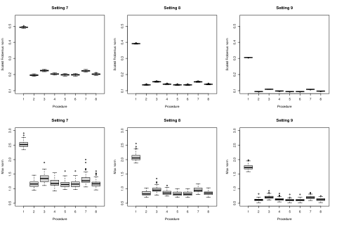
Figure 3: Results from Simulation Settings 7-9. The plots can be interpreted similarly as those in Figure 1.

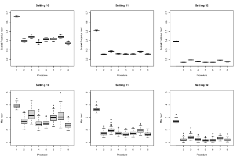
Figure 4: Results from Simulation Settings 10-12. The plots can be interpreted similarly as those in Figure 1.

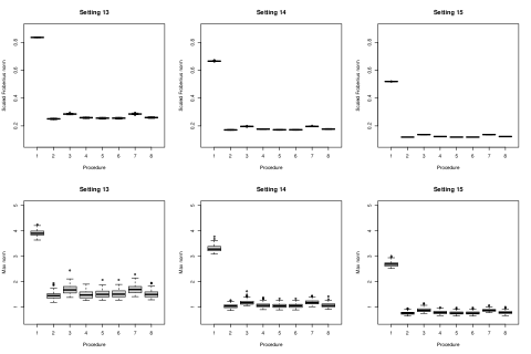
Figure 5: Results from Simulation Settings 13-15. The plots can be interpreted similarly as those in Figure 1.

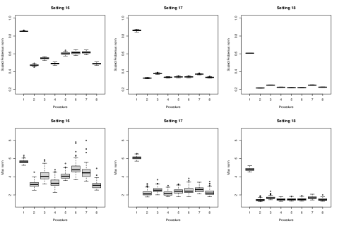
Figure 6: Results from Simulation Settings 16-18. The plots can be interpreted similarly as those in Figure 1.

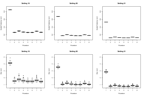
Figure 7: Results from Simulation Settings 19-21. The plots can be interpreted similarly as those in Figure 1.

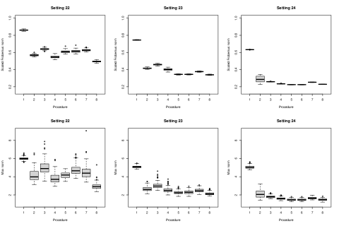
Figure 8: Results from Simulation Settings 22-24. The plots can be interpreted similarly as those in Figure 1.

References

- Abbe et al. [2020] Emmanuel Abbe, Jianqing Fan, Kaizheng Wang, and Yiqiao Zhong. Entrywise eigenvector analysis of random matrices with low expected rank. Annals of Statistics, 48(3):1452–1474, 2020.
- Bartholomew et al. [2008] D J Bartholomew, F Steele, J Galbraith, and I Moustaki. Analysis of multivariate social science data. CRC Press, Boca Raton, FL, 2008.
- Bergner et al. [2022] Yoav Bergner, Peter Halpin, and Jill-Jênn Vie. Multidimensional item response theory in the style of collaborative filtering. Psychometrika, 87(1):266–288, 2022.
- Bhaskar [2016] Sonia A Bhaskar. Probabilistic low-rank matrix completion from quantized measurements. The Journal of Machine Learning Research, 17(1):2131–2164, 2016.
- Biswas et al. [2006] Pratik Biswas, T. Lian, T. Wang, and Yinyu Ye. Semidefinite programming based algorithms for sensor network localization. ACM Transactions on Sensor Networks (TOSN), 2(2):188–220, 2006.
- Boucheron et al. [2013] Stéphane Boucheron, Gábor Lugosi, and Pascal Massart. Concentration inequalities: A nonasymptotic theory of independence. Oxford University Press, Oxford, England, 2013.
- Cai and Zhou [2016] T Tony Cai and Wen-Xin Zhou. Matrix completion via max-norm constrained optimization. Electronic Journal of Statistics, 10(1):1493–1525, 2016.
- Cai and Zhou [2013] Tony Cai and Wen-Xin Zhou. A max-norm constrained minimization approach to 1-bit matrix completion. Journal of Machine Learning Research, 14(1):3619–3647, 2013.
- Candès and Recht [2009] Emmanuel J Candès and Benjamin Recht. Exact matrix completion via convex optimization. Foundations of Computational Mathematics, 9(6):717–772, 2009.
- Candès and Tao [2010] Emmanuel J Candès and Terence Tao. The power of convex relaxation: Near-optimal matrix completion. IEEE Transactions on Information Theory, 56(5):2053–2080, 2010.
- Cao and Xie [2015] Yang Cao and Yao Xie. Poisson matrix recovery and completion. IEEE Transactions on Signal Processing, 64(6):1609–1620, 2015.
- Cape et al. [2019] Joshua Cape, Minh Tang, and Carey E Priebe. The two-to-infinity norm and singular subspace geometry with applications to high-dimensional statistics. Annals of Statistics, 47(5):2405–2439, 2019.
- Chatterjee [2015] Sourav Chatterjee. Matrix estimation by universal singular value thresholding. The Annals of Statistics, 43(1):177–214, 2015.
- Chen and Li [2022] Yunxiao Chen and Xiaoou Li. Determining the number of factors in high-dimensional generalized latent factor models. Biometrika, 109(3):769–782, 2022.
- Chen et al. [2020a] Yunxiao Chen, Xiaoou Li, and Siliang Zhang. Structured latent factor analysis for large-scale data: Identifiability, estimability, and their implications. Journal of the American Statistical Association, 115(532):1756–1770, 2020a.
- Chen et al. [2021] Yunxiao Chen, Chengcheng Li, and Gongjun Xu. A note on statistical inference for noisy incomplete 1-bit matrix. arXiv preprint arXiv:2105.01769, 2021.
- Chen et al. [2019] Yuxin Chen, Jianqing Fan, Cong Ma, and Yuling Yan. Inference and uncertainty quantification for noisy matrix completion. Proceedings of the National Academy of Sciences, 116(46):22931–22937, 2019.
- Chen et al. [2020b] Yuxin Chen, Yuejie Chi, Jianqing Fan, Cong Ma, and Yuling Yan. Noisy matrix completion: Understanding statistical guarantees for convex relaxation via nonconvex optimization. SIAM Journal on Optimization, 30(4):3098–3121, 2020b.
- Chernozhukov et al. [2021] Victor Chernozhukov, Christian Hansen, Yuan Liao, and Yinchu Zhu. Inference for low-rank models. arXiv preprint arXiv:2107.02602, 2021.
- Davenport et al. [2014] Mark A Davenport, Yaniv Plan, Ewout Van Den Berg, and Mary Wootters. 1-bit matrix completion. Information and Inference: A Journal of the IMA, 3:189–223, 2014.
- Feuerverger et al. [2012] Andrey Feuerverger, Yu He, and Shashi Khatri. Statistical significance of the Netflix challenge. Statistical Science, 27:202–231, 2012.
- Goldberg et al. [1992] David Goldberg, David Nichols, Brian M Oki, and Douglas Terry. Using collaborative filtering to weave an information tapestry. Communications of the ACM, 35(12):61–70, 1992.
- Haberman [2008] Shelby J Haberman. When can subscores have value? Journal of Educational and Behavioral Statistics, 33(2):204–229, 2008.
- Han et al. [2020] Ruijian Han, Rougang Ye, Chunxi Tan, and Kani Chen. Asymptotic theory of sparse bradley–terry model. Annals of Applied Probability, 30:2491–2515, 2020.
- Han et al. [2022] Ruijian Han, Yiming Xu, and Kani Chen. A general pairwise comparison model for extremely sparse networks. Journal of the American Statistical Association, pages 1–11, 2022.
- Harper and Konstan [2015] F Maxwell Harper and Joseph A Konstan. The movielens datasets: History and context. Acm transactions on interactive intelligent systems (tiis), 5(4):1–19, 2015.
- Jain et al. [2013] Prateek Jain, Praneeth Netrapalli, and Sujay Sanghavi. Low-rank matrix completion using alternating minimization. In Proceedings of the forty-fifth annual ACM symposium on Theory of computing, pages 665–674, 2013.
- Jayasumana et al. [2019] Anura P Jayasumana, Randy Paffenroth, Gunjan Mahindre, Sridhar Ramasamy, and Kelum Gajamannage. Network topology mapping from partial virtual coordinates and graph geodesics. IEEE/ACM Transactions on Networking, 27(6):2405–2417, 2019.
- Keshavan et al. [2010] Raghunandan H Keshavan, Andrea Montanari, and Sewoong Oh. Matrix completion from noisy entries. Journal of Machine Learning Research, 11:2057–2078, 2010.
- Klopp [2014] Olga Klopp. Noisy low-rank matrix completion with general sampling distribution. Bernoulli, 20(1):282–303, 2014.
- Klopp et al. [2015] Olga Klopp, Jean Lafond, Eric Moulines, and Joseph Salmon. Adaptive multinomial matrix completion. Electronic Journal of Statistics, 9(2):2950–2975, 2015.
- Koltchinskii et al. [2011] Vladimir Koltchinskii, Karim Lounici, and Alexandre B Tsybakov. Nuclear-norm penalization and optimal rates for noisy low-rank matrix completion. The Annals of Statistics, 39(5):2302–2329, 2011.
- Masters and Wright [1984] Geofferey N Masters and Benjamin D Wright. The essential process in a family of measurement models. Psychometrika, 49(4):529–544, 1984.
- McRae and Davenport [2021] Andrew D McRae and Mark A Davenport. Low-rank matrix completion and denoising under Poisson noise. Information and Inference: A Journal of the IMA, 10(2):697–720, 2021.
- Negahban and Wainwright [2012] Sahand Negahban and Martin J Wainwright. Restricted strong convexity and weighted matrix completion: Optimal bounds with noise. Journal of Machine Learning Research, 13(1):1665–1697, 2012.
- OECD [2019a] OECD. PISA 2018 assessment and analytical framework. OECD Publishing, Paris, France, 2019a.
- OECD [2019b] OECD. PISA 2018 techinical report. OECD Publishing, Paris, France, 2019b.
- Ortega and Rheinboldt [2000] James M Ortega and Werner C Rheinboldt. Iterative solution of nonlinear equations in several variables. SIAM, Philadelphia, PA, 2000.
- Reckase [2009] Mark Reckase. Multidimensional item response theory. Springer, New York, NY, 2009.
- Robin et al. [2019] Geneviève Robin, Julie Josse, Éric Moulines, and Sylvain Sardy. Low-rank model with covariates for count data with missing values. Journal of Multivariate Analysis, 173:416–434, 2019.
- Robin et al. [2020] Geneviève Robin, Olga Klopp, Julie Josse, Éric Moulines, and Robert Tibshirani. Main effects and interactions in mixed and incomplete data frames. Journal of the American Statistical Association, 115(531):1292–1303, 2020.
- Skrondal and Rabe-Hesketh [2004] Anders Skrondal and Sophia Rabe-Hesketh. Generalized latent variable modeling: Multilevel, longitudinal, and structural equation models. CRC Press, Boca Raton, FL, 2004.
- Tropp [2012] Joel A Tropp. User-friendly tail bounds for sums of random matrices. Foundations of computational mathematics, 12(4):389–434, 2012.
- Tropp et al. [2015] Joel A Tropp et al. An introduction to matrix concentration inequalities. Foundations and Trends® in Machine Learning, 8(1-2):1–230, 2015.
- Wedel et al. [2003] Michel Wedel, Ulf Böckenholt, and Wagner A Kamakura. Factor models for multivariate count data. Journal of Multivariate Analysis, 87(2):356–369, 2003.
- Wedin [1972] P. Wedin. Perturbation bounds in connection with singular value decomposition. BIT Numerical Mathematics, 12:99–111, 1972.
- Xia and Yuan [2021] Dong Xia and Ming Yuan. Statistical inferences of linear forms for noisy matrix completion. Journal of the Royal Statistical Society: Series B (Statistical Methodology), 83(1):58–77, 2021.
- Zhang et al. [2020] Haoran Zhang, Yunxiao Chen, and Xiaoou Li. A note on exploratory item factor analysis by singular value decomposition. Psychometrika, 85(2):358–372, 2020.