Informative Initialization and Kernel Selection Improves t-SNE for Biological Sequences

Abstract

The t-distributed stochastic neighbor embedding (t-SNE) is a method for interpreting high dimensional (HD) data by mapping each point to a low dimensional (LD) space (usually two-dimensional). It seeks to retain the structure of the data. An important component of the t-SNE algorithm is the initialization procedure, which begins with the random initialization of an LD vector. Points in this initial vector are then updated to minimize the loss function (the KL divergence) iteratively using gradient descent. This leads comparable points to attract one another while pushing dissimilar points apart. We believe that, by default, these algorithms should employ some form of informative initialization. Another essential component of the t-SNE is using a kernel matrix, a similarity matrix comprising the pairwise distances among the sequences. For t-SNE-based visualization, the Gaussian kernel is employed by default in the literature. However, we show that kernel selection can also play a crucial role in the performance of t-SNE.

In this work, we assess the performance of t-SNE with various alternative initialization methods and kernels, using four different sets, out of which three are biological sequences (nucleotide, protein, etc.) datasets obtained from various sources, such as the well-known GISAID database for sequences of the SARS-CoV-2 virus. We perform subjective and objective assessments of these alternatives. We use the resulting t-SNE plots and $k$-ary neighborhood agreement ($k$-ANA) to evaluate and compare the proposed methods with the baselines. We show that by using different techniques, such as informed initialization and kernel matrix selection, that t-SNE performs significantly better. Moreover, we show that t-SNE also takes fewer iterations to converge faster with more intelligent initialization.

I Introduction

The quantity of high dimensional data sets in genomic sequencing necessitates dimensionality reduction techniques and ways to aid in creating data visualizations. Principal component analysis (PCA) and independent component analysis (ICA) are standard dimensionality reduction techniques. Among them, the t-distributed stochastic neighbor embedding (t-SNE) introduced by van der Maaten and Hinton (2008) [1] has recently gained popularity, especially in the natural sciences, due to its ability to handle large amounts of data and its use for dimensionality reduction while preserving the structure of data. It is typically used to create a two-dimensional embedding of high-dimensional data to simplify viewing while keeping its overall structure. Despite its enormous empirical success, the theory behind t-SNE remains to be seen.

This paper demonstrates the effect of informed initialization on the step-wise process (incremental performance, convergence, etc.) of the t-SNE algorithm. We also review the impact of different kernels on t-SNE for various types of biological (nucleotide, protein, etc.) sequence data, including SARS-CoV-2 sequences. The vast global spread of pandemics like COVID-19 provided the impetus for this research, pushing viral sequence analysis into the “Big Data” realm. This leads to challenges in reducing high-dimensional data to low-dimensional space, not just to conserve computational resources when using it in cutting-edge methods like machine learning, but also to improve visualization.

The severe acute respiratory syndrome coronavirus 2 (SARS-CoV-2) virus is a member of the genus Betacoronavirus, and its genetic material is a single positive-strand RNA [2]. Its viral genome (Gene ID—MN908947) has roughly $29,881$ nucleotides [3]. The virus has a double-layered lipid envelope with four structural proteins, S, M, E, and N, in its structure. Most of the mutations related to SARS-CoV-2 occur in the spike region [4].

In this work, we use four datasets, of which three sets are biological sequences, to assess the effect of informed initialization and kernel selection on t-SNE. Firstly, we use a toy dataset as a proof of concept. Among others, there is a set of 7000 SARS-CoV-2 spike protein sequences obtained from the well-known GISAID database. The COVID-19 pandemic has generated a renewed interest in the larger family Coronaviridae, among which SARS-CoV-2 is a member, along with others such as the original severe acute respiratory syndrome and the middle-eastern respiratory syndrome coronaviruses [5]. Since the family Coronaviridae affects a wider variety of hosts, it is often of interest to characterize such viral sequences with the primary host that it affects. Hence, the third dataset used contains the host for each sequence. Finally, sometimes researchers only obtain such data in the form of short reads (when no reference genome is available, for example). To simulate this scenario, our fourth dataset is obtained by taking a set of $\approx$10K full-length nucleotide sequences of SARS-CoV-2, and simulating the process of sequencing, Illumina reads from each such nucleotide sequence.

In this paper, our contributions are the following:

1. We convert the biological sequences to a fixed-length numerical representation, afterward, we compute different kernel matrices and show their effect along with several initialization methods on the quality of t-SNE.

2. We show that the Kernel selection can play an important role and should be considered carefully rather than using the typical Gaussian kernel for t-SNE computation.

3. We show that random initialization is inefficient for t-SNE computation. Alternatively, the Ensemble approach is a better choice to start with as an initial solution than the Random, Principal Component Analysis (PCA), and Independent Component Analysis (ICA) approaches.

4. We evaluate the performance of the t-SNE using subjective (t-SNE plots) and objective ($AUC_{RNX}$ ) criteria, and report results for different kernel computation methods along with different initialization approaches.

5. We show that our proposed setting that includes the use of Laplacian kernel, along with ensemble initialization, outperforms the typical Gaussian and Isolation kernel-based methods in terms of $AUC_{RNX}$.

The rest of the paper is organized as follows: Section II contains the related work for the t-SNE computation problem. Our proposed solution is given in Section III. The dataset statistics, along with the experimental setup details, are given in Section IV. Our results are reported in Section V. Finally, we conclude the paper in Section VI.

II Related Work

The task of data visualization is crucial. This work has been made easier using t-SNE, which was first introduced in [6]. Authors in [7] use it to show distinct variations in coronavirus protein sequence data. It was also discovered that employing k-means to cluster SARS-CoV-2 protein sequences is similar to the patterns shown in t-SNE plots [8, 9]. Authors in [10] present a theoretical feature of SNE (a forerunner to t-SNE) requiring that global minimizers quantitatively separate clusters. However, their finding is only nontrivial when the number of clusters is much greater than the number of points per cluster, which is not a reasonable assumption in general.

Authors in [11] show the importance of initialization in UMAP and t-SNE. With informed initialization, t-SNE performs as well as UMAP. However, they have yet to consider the importance of kernel selection. In [12], a decentralized data stochastic neighbor embedding (dSNE) is developed, which is beneficial for visualizing decentralized data. In [13], authors propose a deferentially private dSNE (DP-dSNE) variant. Both dSNE and DP-dSNE use similarity to map the data points from distinct places. The dSNE and DP-dSNE approaches come in handy when data cannot be shared due to privacy issues. Although current t-SNE approaches are effective on popular datasets like MNIST, it is unclear if they can be applied to large datasets of biological sequences.

III Proposed Approach

In this section, we first discuss the method to convert the sequences into a fixed-length numerical representation. We then describe the different kernel computation methods. Finally, we describe initialization approaches for the t-SNE.

III-A Numerical Embedding Generation

Since t-SNE operates on the numerical vectors/embeddings, the first step is to convert the sequences into fixed-length numerical representations. For this purpose, we use a recently proposed method called Spike2Vec [14]. Given a sequence, Spike2Vec generates a fixed-length numerical representation using the concept of $k$-mers (also called n-gram). It uses the idea of the sliding window to generate substrings (called mers) of length $k$ (size of the window). For a set of $k$-mer for a biological sequence, we generate a feature vector of length $|\Sigma|^{k}$ (where $\Sigma$ corresponds to the set of alphabets “amino acids” or nucleotide in the sequence), which contains the frequency/count of each $k$-mer.

III-B t-SNE computation pipeline

The overall pipeline of our model is shown in Figure 1. In the t-SNE computation pipeline, there are three steps involved, namely (1) Kernel matrix computation, (2) Solution Initialization, and (3) Gradient Descent.

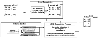
Figure 1: Overall pipeline of our model. Given the input data (A), we first compute the kernel matrix (P) using different kernel functions. We then Initialize a solution (Y) using different initialization approaches. Later we apply Gradient Descent to get the low dimensional representation of the data.

III-B1 Kernel Functions

For kernel matrix computation, we use four different kernel functions, which are described below, and also the process is shown in the first box of Figure 1.

Gaussian Kernel [15]

The N-dimensional Gaussian kernel is computed for any number of points by computing each Kernel coordinates and their distance to the chosen points, then taking the Gaussian function of these distances. In 2D, the Gaussian Kernel is defined as: $\mathcal{K}\left(x,y\right)=\exp\left(\frac{-\left\|x-y\right\|^{2}}{2\sigma^{2}}\right)$, where the width of the Kernel is defined by $sigma$, we computed the difference using Squared Euclidean distance with a perplexity value of $250$ for our trials, and we are tweaking $sigma$. The Gaussian Kernel is a default Kernel used in the t-SNE implementation. We use this as a baseline to evaluate the performance of other Kernel.

Isolation Kernel  [16]

It is a data-dependent kernel that is quick to compute because it just has one parameter. It adjusts to the local density distribution, unlike the Gaussian kernel. For given two points $x$, $y\in\mathrm{R}^{d}$, the Isolation kernel of $x$ and $y$ with respect to $\mathrm{D}$ is defined to be the expectation taken over the probability distribution on all partitioning $\mathrm{H}\in\mathrm{H_{\psi}}(\mathrm{D})$ which both $x$ and $y$ fall into the same isolating partition $\theta[z]\in\mathrm{H},z\in D$ given by: $K_{\psi}(x,y\mid D)=\mathbb{E}_{\mathbb{H}_{\psi}(D)}[\mathbb{1}(x,y\in\theta[z]\mid\theta[z]\in H)]$.

Laplacian Kernel [17]

The Laplacian kernel function gives the relationship between two input feature vectors $x$ and $y$ in infinite-dimension space. Its value ranges between $0$ and $1$ where, $1$ denotes $x$ and $y$ are similar. Can be denoted by the following: $k(x,y)=\exp\left(-\frac{1}{2\sigma^{2}}\|x-y\|_{1}\right)$, where $\mathrm{x}$ and $\mathrm{y}$ are the input vectors and $\|x-y\|_{1}$ is the Manhattan distance between the input vectors.

Approximate Kernel [18]

This kernel offers a mechanism to compare two sequences’ similarities by computing a spectrum based on the number of matches $k$ and mismatches $m$ between $k$-mers of two sequences. Given a pair of the sequence $X$ and $Y$, the spectrum (frequency count-based vector of $k$-mers) between any two sequences will have a length equal to the size of more significant length sequences between $X$ and $Y$, which will contain the counts of matches and mismatches between characters in the sequence $k$-mers. This method computes $n\times n$ kernel matrix based on the dot product of vectors. We use $k=3$ and $m=0$ for computing this kernel.

III-B2 Solution Initialization

It is an important component of the t-SNE computation process. For the initialization of t-SNE, we use the following four techniques, also shown in the second box of Figure 1.

Random Initialization

Random numbers are assigned to the $N\times 2$ matrix, where N is the total number of sequences.

Principle Component Analyses (PCA) [19]

Singular Value Decomposition reduces the data’s dimensionality and projects it to a lower dimensional environment. We are not using PCA as a dimensionality reduction method here. Rather, we use it to get intelligent initial t-SNE vectors(initialization). Here we get $N\times 2$ matrix as output when numerical embedding is provided as input to PCA. This low-dimensional output is used to initialize the solution for the t-SNE algorithm.

Independent Component Analyses (ICA) [20]

ICA establishes two essential assumptions, i.e., statistical independence and non-Gaussian distribution property, among the components. In a semantic sense, the information about $x$ (original data) does not provide information about $y$ (new data comprised of independent components), and vice versa. Its goal is to separate the data by transforming the input space into a maximally independent basis. More formally, this corresponds to $p(x,y)=p(x)p(y)$, where the probability distribution of x is represented by p(x), and p(x,y) represents the joint distribution of x and y.

Ensemble

We took the average for $N\times 2$ matrices generated by PCA and ICA in this method. Initialize the solution in t-SNE with the generated averaged matrix.

III-B3 Gradient Descent

Ultimately, we use gradient descent to optimize the t-SNE-based 2D representation. As shown in the last part of Figure 1, we set the parameters like learning rate, momentum, and Iteration. KL divergence is used to measure the distance between two distributions (Distribution among distances in the data points in LD and HD). Taking the cost function’s derivative and calculating gradient descent, we keep updating the initial solution $Y$ to get the optimal solution. Finally, we apply t-distribution on low-dimension distribution, which gives us a longer tail to give better visualization.

IV Experimental Setup

In this section, we first discuss the dataset statistics. After that, we report the goodness metrics used to evaluate the performance of t-SNE. All experiments are performed on Intel (R) Core i5 system with a 2.40 GHz processor and $32$ GB memory. The code and dataset used in this study are available online https://github.com/pchourasia1/tSNE_Informed_Initialization.

IV-A Dataset Statistics

This section discusses the detailed description and statistics of datasets used for experiments.

IV-A1 Circle Dataset

Using a straightforward toy dataset, we can demonstrate the significance of random and non-random (informed) initialization. To create Kernel matrices, we collected $7000$ points from a circle with some additional Gaussian noise.

IV-A2 Spike Sequence Dataset

The spike sequences are taken from GISAID , a well-known database. The entire retrieved sequences are $7000$, including $22$ lineages of virus. The detail of each lineage, i.e., name (count/distribution), in the dataset, is as follow B.1.1.7 (3369), B.1.617.2 (875), AY.4 (593), B.1.2 (333), B.1 (292), B.1.177 (243), P.1 (194), B.1.1 (163), B.1.429 (107), B.1.526 (104), AY.12 (101), B.1.160 (92), B.1.351 (81), B.1.427 (65), B.1.1.214 (64), B.1.1.519 (56), D.2 (55), B.1.221 (52), B.1.177.21 (47), B.1.258 (46), B.1.243 (36), and R.1 (32).

IV-A3 Host Dataset

This data is taken from [5], which comprised $5558$ spike sequences and coronavirus hosts as class labels. The count of each host (class label) is following: Bats (153), Bovines (88), Cats (123), Cattle (1), Equine (5), Fish (2), Humans (1813), Pangolins (21), Rats (26), Turtle (1), Weasel (994), Birds (374), Camels (297), Canis (40), Dolphins (7), Environment (1034), Hedgehog (15), Monkey (2), Python (2), Swines (558), and Unknown (2). Length of Spike2Vec based feature vector is $13824$.

IV-A4 Short Read Dataset

This dataset is generated by taking $10181$ SARS-CoV-2 nucleotide sequences and simulating short reads from each sequence using inSilicoSeq  with the miseq model (all other settings were default settings). The lineages/class labels (count/distribution) in this dataset is as follows: B.1.1.7 (2587), B.1.617.2 (1198), AY.4 (1167), AY.43 (412), AY.25 (275), B.1.2 (253), AY.44 (249), B.1 (200), B.1.177 (184), AY.3 (166), P.1 (137), B.1.1 (128), B.1.526 (112), AY.9 (108), AY.5 (96), AY.29 (86), AY.39 (85), B.1.429 (81), B.1.160 (79), Others (2578). There are $496$ unique lineages for $10181$ sequences.

IV-B Evaluation Metrics

We evaluate the t-SNE in two ways including subjective and objective evaluation. We plot t-SNE-based 2D visual representation for subjective evaluation to evaluate the performance. For objective evaluation, we use a technique called $k$-ary neighborhood agreement ($k$-ANA) method  [16] to analyze the t-SNE model’s performance objectively. Given the original high dimensional (HD) data and the equivalent low dimensional (LD) data for this assessment method ($2$D data computed using the t-SNE approach), the $k$-ANA approach verifies the neighborhood agreement ($Q$) between HD and LD. It gets the intersection on the number of neighbors (for various $k$ nearest neighbors). In a formal setting:

$$Q(k)=\sum_{i=1}^{n}\frac{1}{nk}\left|kNN\left(x_{i}\right)\cap kNN\left(x_{i}^{\prime}\right)\right|$$ (1)

where $k$NN($x$) is the set of $k$ nearest neighbors of $x$ in high-dimensional and $k$NN($x^{\prime}$) is the set of $k$ nearest neighbors of $x$ in low-dimensional (LD). We employed a quality evaluation technique that quantifies neighborhood preservation and is denoted by R($k$), which evaluates on a scalar metric if neighbors are preserved [21] in low dimensions using Equation 1. In a formal setting: $R(k)=\frac{(n-1)Q(k)-k}{n-1-k}$. The value of R($k$) ranges from $0$ to $1$, with a higher score indicating better neighborhood preservation in LD space. We computed $R(k)$ for $k\in\{1,2,3,...,99\}$ in our experiment, then looked at the area under the curve (AUC) created by $k$ and R($k$). Finally, we compute the area under the $R(k)$ curve in the log plot ($AUC_{RNX}$) [22] to aggregate the performance of various k-ANN. More formally, $AUC_{RNX}=\frac{\Sigma_{k}\frac{R(k)}{k}}{\Sigma_{k}\frac{1}{k}}$, where $AUC_{RNX}$ is an average quality weight for $k$ closest neighbors.

V Results and Discussion

This section reports the results of t-SNE for different kernels and initialization methods. The deformed circular data with isolation and Laplacian kernel was created using the t-SNE method with the random initialization, also shown in Figure 2(a). In this instance, it is clear that the overall structure was not maintained; in fact, gradient descent in t-SNE merely brings near neighbors closer and is hardly affected by the overall arrangement of points. While using PCA (frequently suggested for initialization in t-SNE), it restores the original circle and significantly enhances the t-SNE result (see Figure 2(b)). While recovering the original circle for all $3$ kernels, informed initialization (PCA) simultaneously significantly improves the outcomes. Thus, it is clear that the closed one-dimensional manifold—the circle—can only be faithfully represented with informative initialization.

(a) Random Initialization

(b) PCA Initialization

Figure 2: t-SNE plots comparison for different kernel matrices with Random and PCA initialization for Circle toy dataset using Gaussian, Isolation, and Laplacian kernels, respectively.

In Figure 3, using various kernels and initialization strategies, we present the $AUC_{RNX}$ charts for gradient descent iterations ranging from $100$ to $2000$. With ensemble initialization, the Laplacian Kernel outperforms the competition. Based on these results, we suggest a recommendation and avoiding combination in Table I.

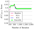
(a) Gaussian Kernel

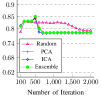
(b) Isolation Kernel

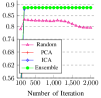
(c) Laplacian Kernel

Figure 3: AUC score of t-SNE for different Kernel methods applied with increasing number of iteration for Circle data. The figure is best seen in color.

In Figure 4, we report the t-SNE plots (for Spike sequence data) using the different kernels (for Spike2Vec-based embedding) and random initialization method. We can observe that the Alpha (B.1.1.7) variation displays unambiguous grouping in most cases. For Gaussian and Isolation kernels, only the alpha variant is clearly separated. The other classes overlap with each other. However, for the Laplacian kernel, we can see smaller groups for other variants, such as Delta (AY.4) and Epsilon (B.1.429).

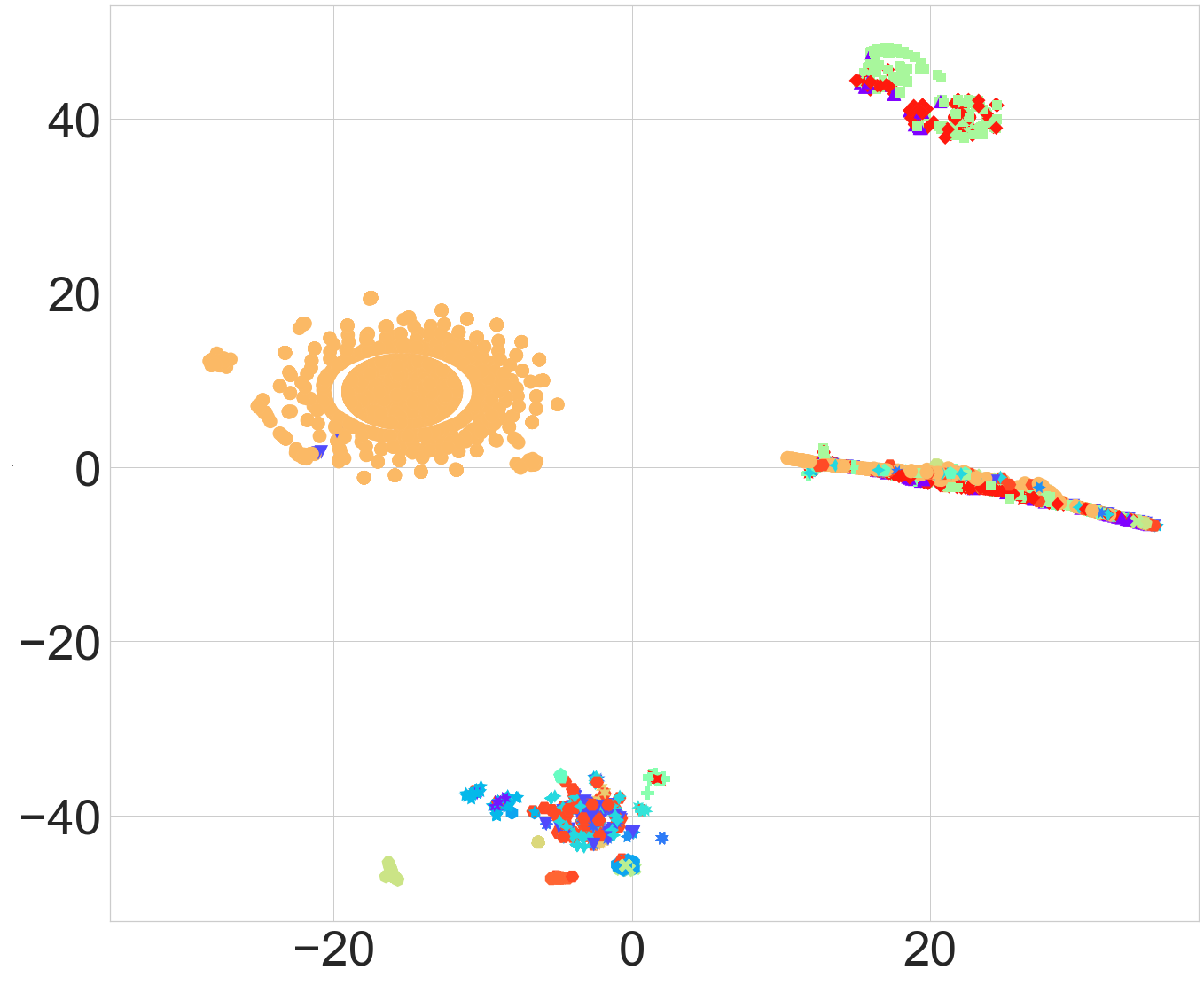
(a) Gaussian

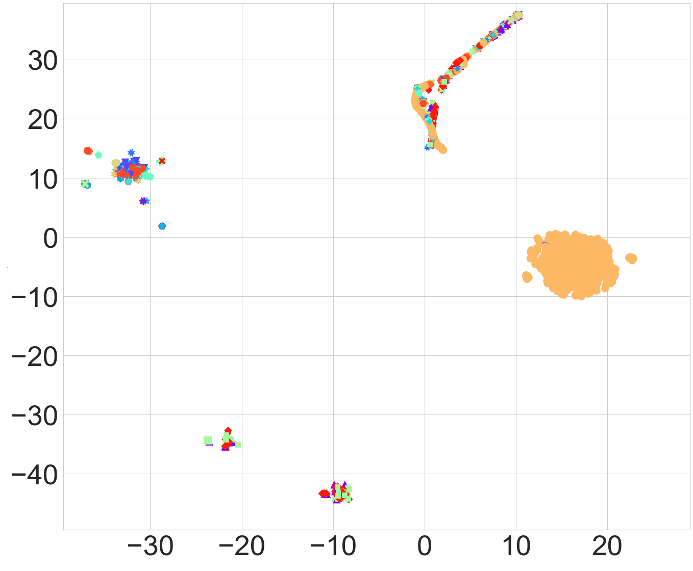
(b) Isolation

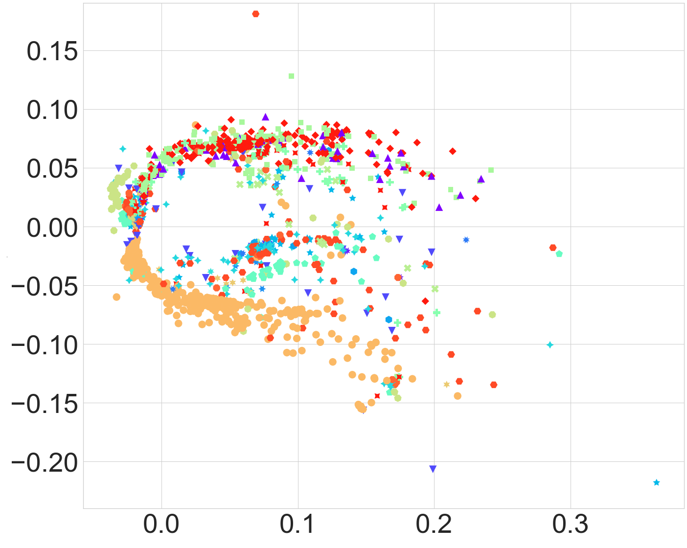
(c) Laplacian

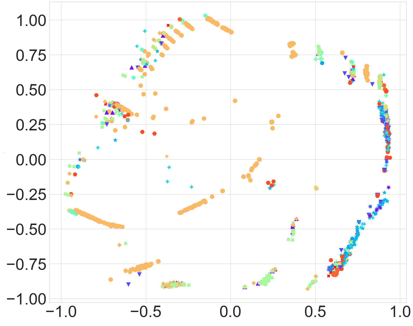
(d) Approximate

Figure 4: t-SNE plots for different kernel matrices with random initialization for Spike Sequence dataset.

Figure 5 shows the results of $AUC_{RNX}$ for different initialization approaches and kernel computation techniques for Spike data. For the Gaussian kernel, all initialization methods perform comparably to each other as the number of iterations increases. Similarly, for the Isolation kernel, we can observe that the random initialization-based approach is worse than other initialization methods. However, the other three (PCA, ICA, and Ensemble) methods seem to perform similarly. At around $1500^{th}$ iteration, the ICA-based initialization gets a spike in $AUC_{RNX}$ compared to the other methods. However, it is not significant as compared to an ensemble. For the Laplacian kernel, the ensemble initialization approach seems to perform better than the other methods, while random initialization performs worst at the start. Moreover, the maximum $AUC_{RNX}$ reported for the Laplacian kernel is the largest among all three kernels, which shows that the Gaussian kernel is the typical kernel used for t-SNE computation, may not be a good choice. Based on this result, We can recommend Laplacian with Ensemble and say Random performs poorly with Isolation and Laplacian Kernel, as mentioned in Table I.

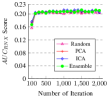
(a) Gaussian Kernel

(b) Isolation Kernel

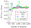
(c) Laplacian Kernel

(d) Approximate Kernel

Figure 5: AUC score of t-SNE for different Kernel methods and initialization with the increasing number of iterations for Spike sequence data. The figure is best seen in color.

In Figure 6, we report the t-SNE plots using the different kernels and random initialization method for Host data. In most cases, the Environment and Human displays unambiguous grouping. For Laplacian, classes overlap with each other. However, for the Approximate kernel, we can see smaller groups for other variants, such as Bird and Swine.

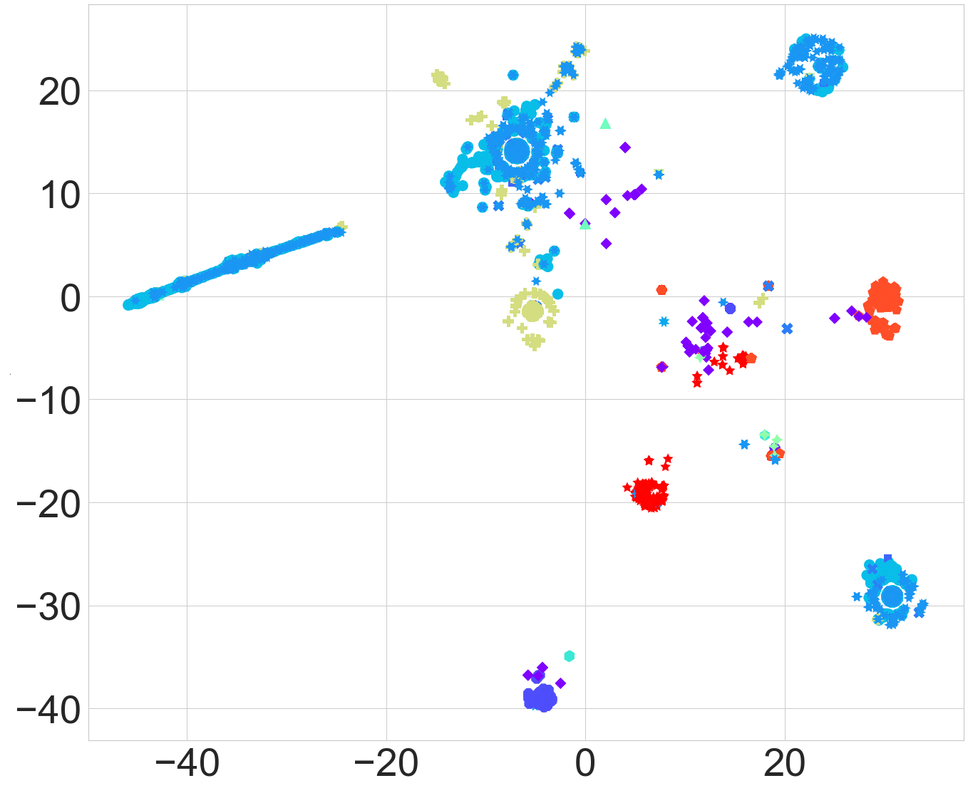
(a) Gaussian

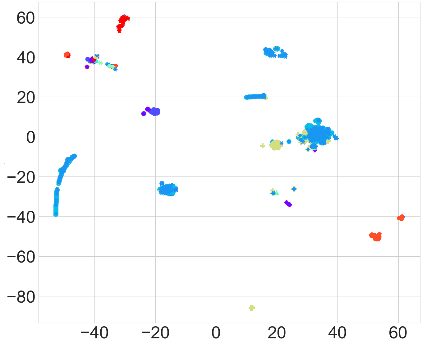
(b) Isolation

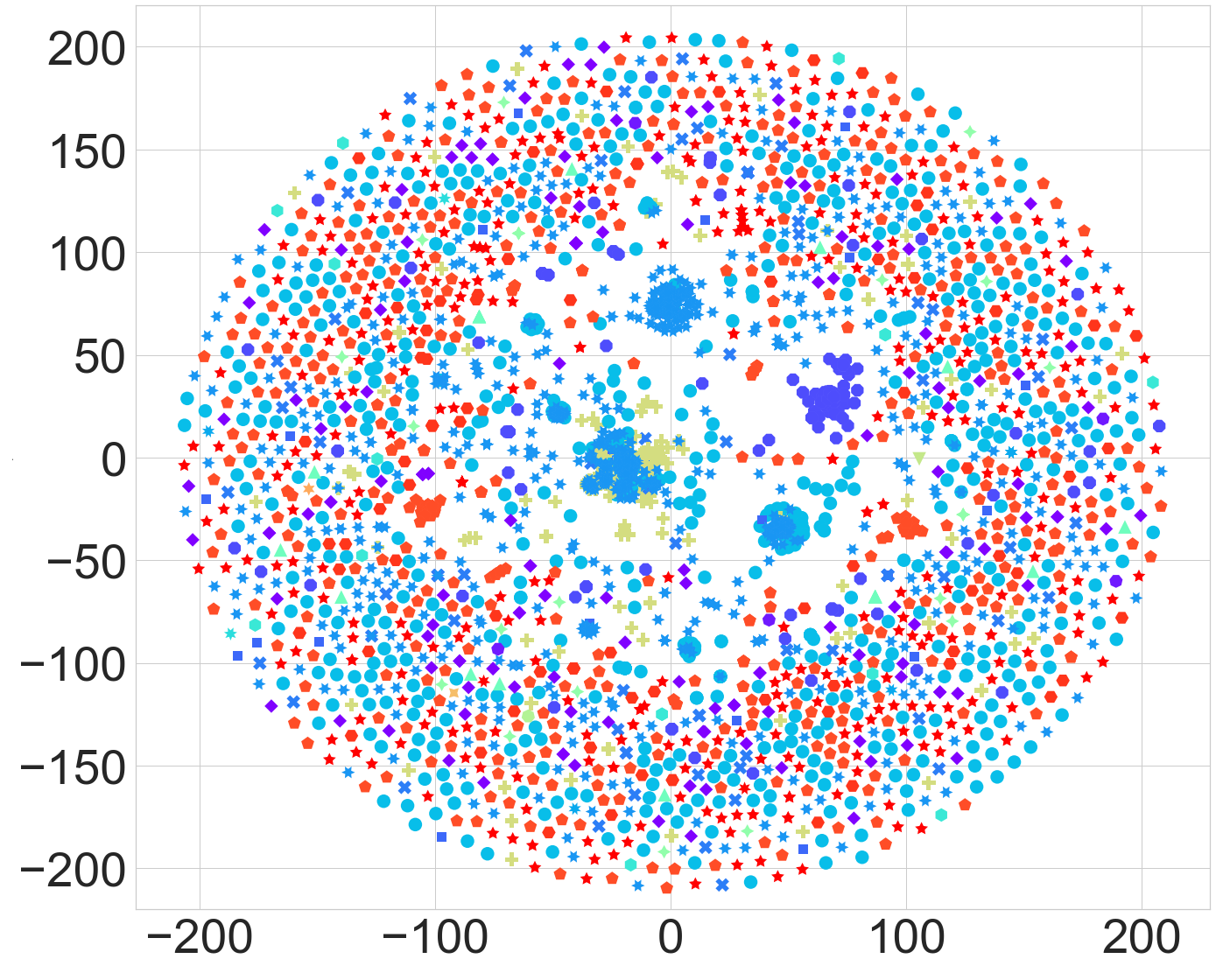
(c) Laplacian

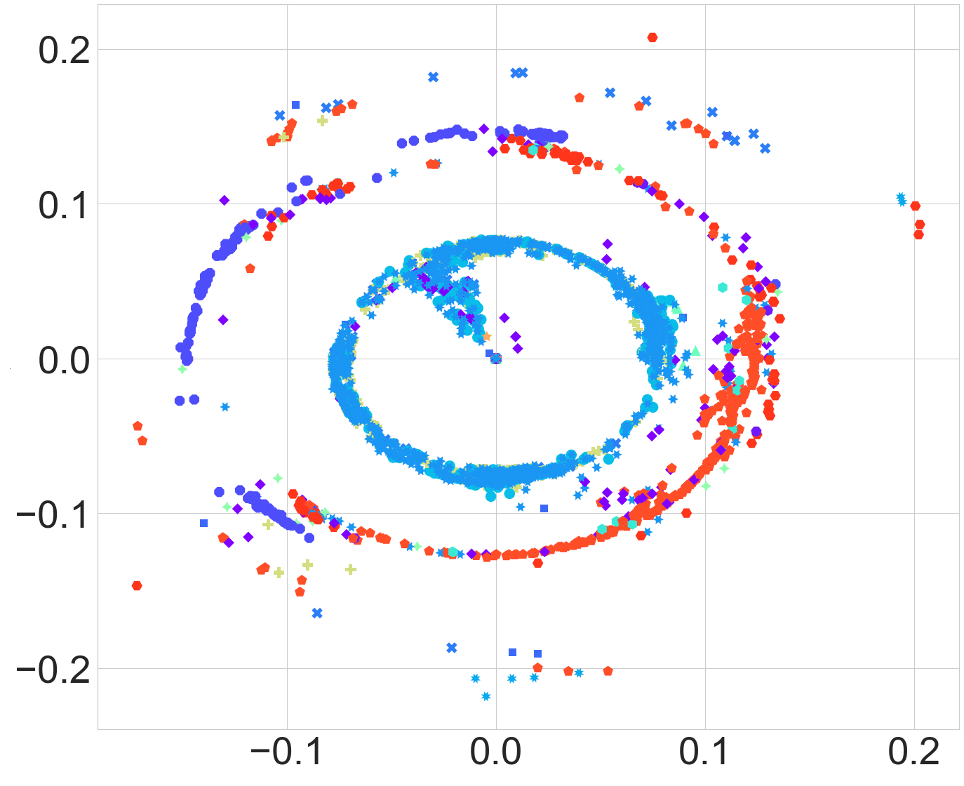
(d) Approximate

Figure 6: t-SNE plots for different kernel matrices with random initialization for Coronavirus Host dataset.

Figure 7 shows the results of $AUC_{RNX}$ for different initialization approaches and kernel computation techniques for Host data. For the Gaussian kernel and Isolation Kernel, all initialization methods perform comparably to each other as the number of iterations increases. In comparison, Laplacian and Approximate are worse and can not be compared. However, among them, random initialization significantly performs worst than other initialization in Laplacian. Ensemble methods seem comparable in general (especially with Approximate kernel). Overall Isolation kernel, with the ensemble initialization approach, seems to perform better than the other methods. In contrast, random initialization with Laplacian and ICA initialization with Approximate Kernel perform worst. The summary is shown in Table I.

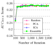
(a) Gaussian Kernel

(b) Isolation Kernel

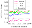
(c) Laplacian Kernel

(d) Approximate Kernel

Figure 7: AUC score of t-SNE for different Kernel with an increasing number of iterations for Coronavirus Host data comprised of 5558 sequences. The figure is best seen in color.

In Figure 8, we report the t-SNE plots using the different kernels (for Spike2Vec-based embedding) and random initialization method for Short Read data. We can see Gaussian and Isolation are somewhat similar, but Laplacian and Approximate are overlapping, and hard to find groups in them. A high number of classes($496$) is one of the reasons.

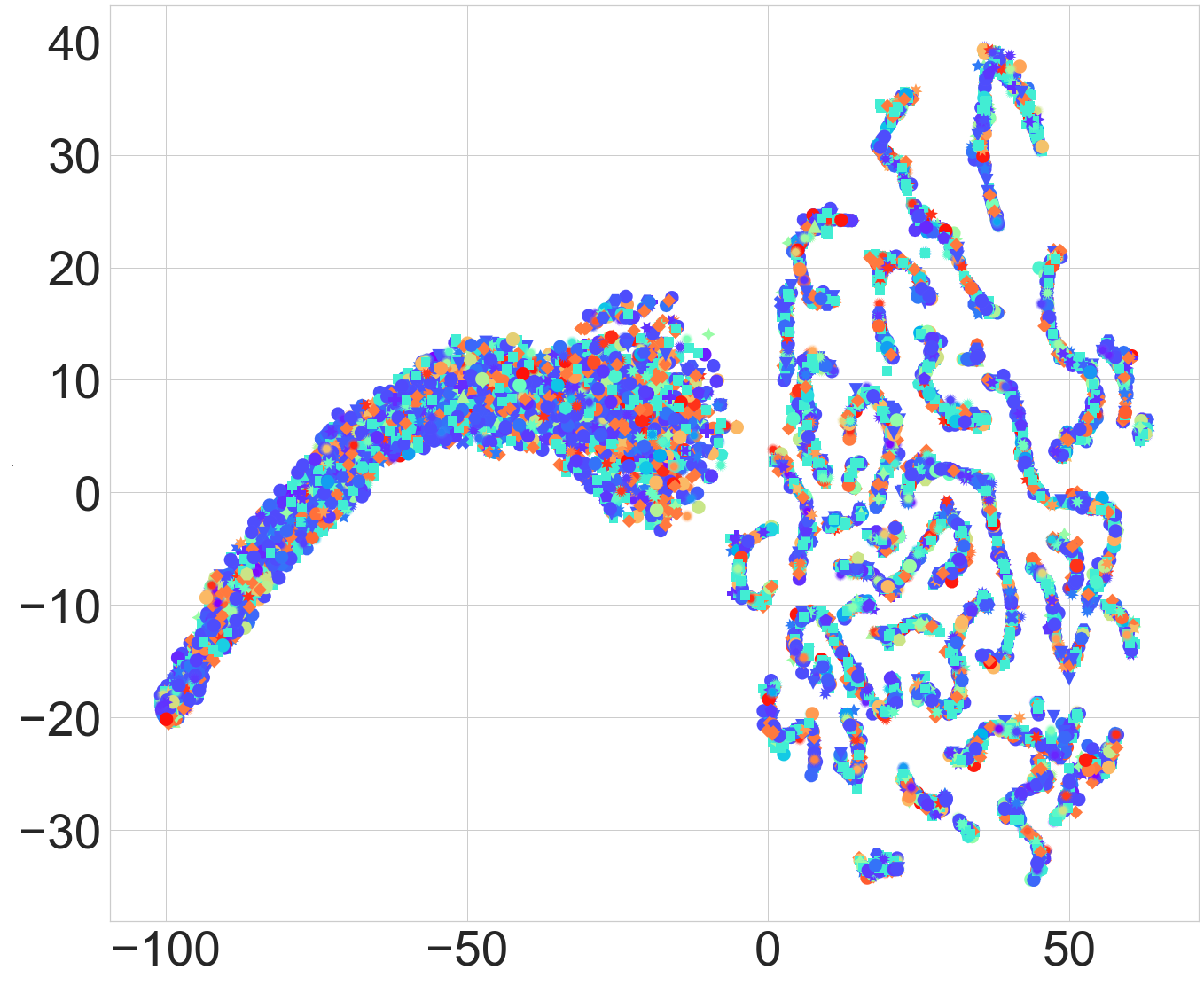
(a) Gaussian

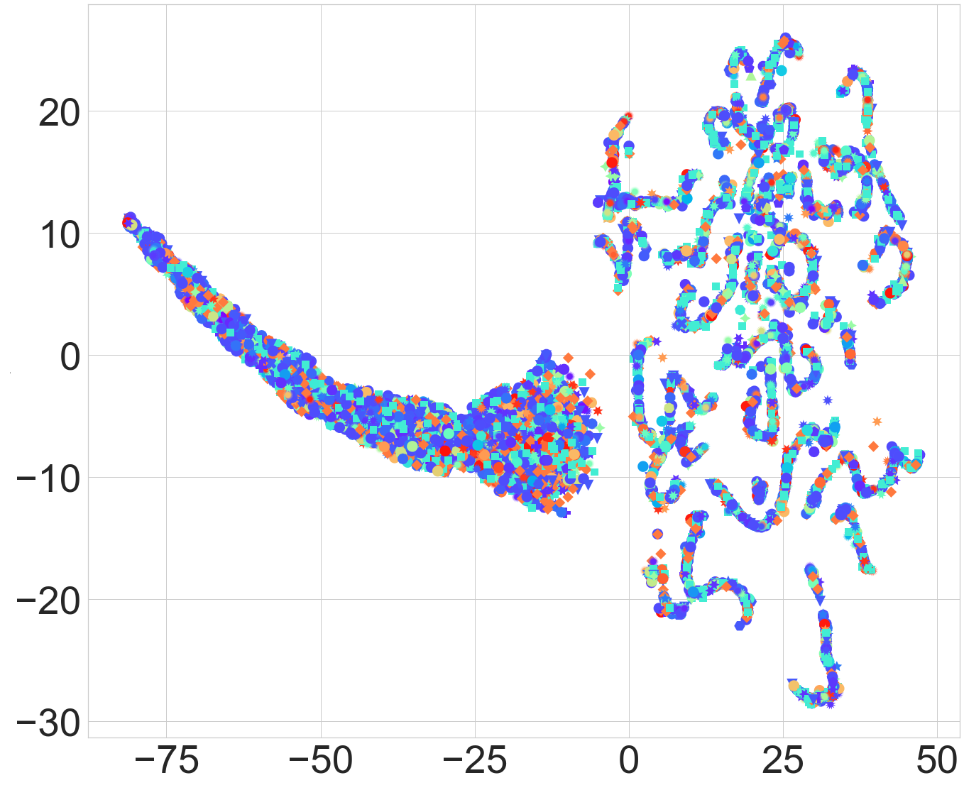
(b) Isolation

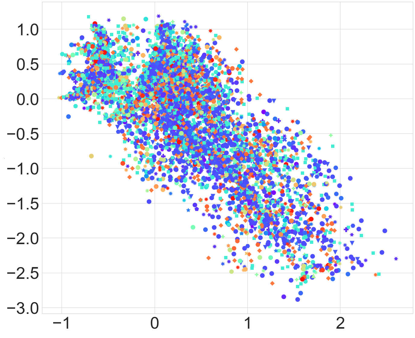
(c) Laplacian

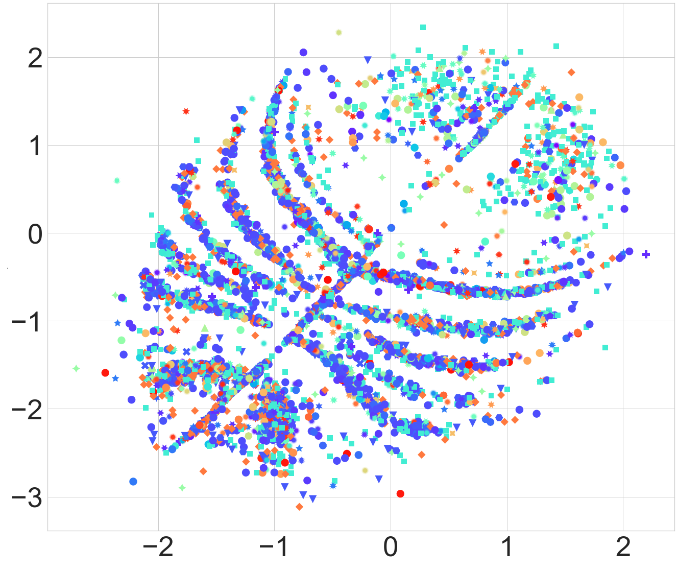
(d) Approximate

Figure 8: t-SNE plots for different kernels with random initialization for Short Read dataset. The legends for $496$ classes are not shown to save space. The figure is best seen in color.

Figure 9 shows the results of $AUC_{RNX}$ for Short Read data. For the Gaussian kernel, all initialization methods perform comparably to each other as the number of iterations increases. Isolation is somewhat close but incomparable with Gaussian, whereas Laplacian and Approximate Kernels are significantly worse. However, among all initialization, Ensemble methods seem to perform better. Overall Gaussian kernel, with the ensemble initialization approach, appears to be a reasonable choice. Conversely, any other Kernel seems not a good choice, as mentioned in the recommendation summary in Table I.

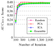
(a) Gaussian Kernel

(b) Isolation Kernel

(c) Laplacian Kernel

(d) Approximate Kernel

Figure 9: AUC score of t-SNE for different Kernel methods and initialization with the increasing number of iterations for Short Read data. The figure is best seen in color.

Dataset	Recommended		Not Recommended
	Kernel	Initialization	Kernel	Initialization
Circle	Laplacian	Ensemble	Isolation	ICA
			Laplacian	Random
Spike	Laplacian	Ensemble	Approximate	PCA
			Isolation	Random
			Laplacian	Random
Host	Isolation	Ensemble	Approximate	ICA
			Laplacian	Random
Short Read	Gaussian	Ensemble	All others	None

TABLE I: Recommendation based on summary of performance ($AUC_{RNX}$) on different dataset.

VI Conclusion

We propose using an ensemble initialization procedure to improve the performance of t-SNE for biological sequences. We show that kernel selection can also play a crucial role along with ensemble initialization to improve the performance of t-SNE. In the future, we will explore more kernels and initialization methods along with other biological data to study the behavior of t-SNE.

References

- [1] G. Hinton and L. van der Maaten, “Visualizing data using t-sne,” J. Mach. Learn. Res., vol. 9, no. Nov, pp. 2579–2605, 2008.
- [2] C. Bai, Q. Zhong, and G. F. Gao, “Overview of sars-cov-2 genome-encoded proteins,” Science China Life Sciences, pp. 1–15, 2021.
- [3] R. Raman, K. J. Patel, and K. Ranjan, “Covid-19: Unmasking emerging sars-cov-2 variants, vaccines and therapeutic strategies,” Biomolecules, vol. 11, no. 7, p. 993, 2021.
- [4] A. C. Walls, Y.-J. Park, M. A. Tortorici, A. Wall, A. T. McGuire, and D. Veesler, “Structure, function, and antigenicity of the sars-cov-2 spike glycoprotein,” Cell, vol. 181, no. 2, pp. 281–292, 2020.
- [5] S. Ali, B. Bello, P. Chourasia, R. T. Punathil, Y. Zhou, and M. Patterson, “Pwm2vec: An efficient embedding approach for viral host specification from coronavirus spike sequences,” MDPI Biology, 2022.
- [6] L. Van der Maaten and G. Hinton, “Visualizing data using t-sne.” Journal of machine learning research, vol. 9, no. 11, 2008.
- [7] S. Ali, B. Sahoo, N. Ullah, A. Zelikovskiy, M. Patterson, and I. Khan, “A k-mer based approach for sars-cov-2 variant identification,” in International Symposium on Bioinformatics Research and Applications, 2021, pp. 153–164.
- [8] S. Ali, Tamkanat-E-Ali, M. A. Khan, I. Khan, and M. Patterson, “Effective and scalable clustering of sars-cov-2 sequences,” in International Conference on Big Data Research (ICBDR), 2021, pp. 1–8.
- [9] Z. Tayebi, S. Ali, and M. Patterson, “Robust representation and efficient feature selection allows for effective clustering of sars-cov-2 variants,” Algorithms, vol. 14, no. 12, p. 348, 2021.
- [10] U. Shaham and S. Steinerberger, “Stochastic neighbor embedding separates well-separated clusters,” arXiv preprint arXiv:1702.02670, 2017.
- [11] D. Kobak and G. C. Linderman, “Initialization is critical for preserving global data structure in both t-sne and umap,” Nature biotechnology, vol. 39, no. 2, pp. 156–157, 2021.
- [12] D. K. Saha, V. D. Calhoun, S. R. Panta, and S. M. Plis, “See without looking: joint visualization of sensitive multi-site datasets.” in IJCAI, 2017, pp. 2672–2678.
- [13] D. K. Saha, V. Calhoun, Y. Du, Z. Fu, S. Panta, S. Kwon, A. Sarwate, and S. Plis, “Privacy-preserving quality control of neuroimaging datasets in federated environment,” Hum Brain Mapp, 2022.
- [14] S. Ali and M. Patterson, “Spike2vec: An efficient and scalable embedding approach for covid-19 spike sequences,” in International Conference on Big Data (Big Data), 2021, pp. 1533–1540.
- [15] G. E. Hinton and S. Roweis, “Stochastic neighbor embedding,” Advances in neural information processing systems, vol. 15, 2002.
- [16] Y. Zhu and K. M. Ting, “Improving the effectiveness and efficiency of stochastic neighbour embedding with isolation kernel,” Journal of Artificial Intelligence Research, vol. 71, pp. 667–695, 2021.
- [17] M. R. Hajiaboli, M. O. Ahmad, and C. Wang, “An edge-adapting laplacian kernel for nonlinear diffusion filters,” IEEE Transactions on Image Processing, vol. 21, no. 4, pp. 1561–1572, 2011.
- [18] S. Ali, B. Sahoo, M. A. Khan, A. Zelikovsky, I. U. Khan, and M. Patterson, “Efficient approximate kernel based spike sequence classification,” IEEE/ACM Transactions on Computational Biology and Bioinformatics, 2022.
- [19] S. Wold, K. Esbensen, and P. Geladi, “Principal component analysis,” Chemometrics and intelligent laboratory systems, vol. 2, no. 1-3, pp. 37–52, 1987.
- [20] A. Hyvärinen and E. Oja, “Independent component analysis: algorithms and applications,” Neural networks, vol. 13, no. 4-5, pp. 411–430, 2000.
- [21] J. Lee, D. Peluffo-Ordóñez, and M. Verleysen, “Multi-scale similarities in stochastic neighbour embedding: Reducing dimensionality while preserving both local and global structure,” Neurocomputing, vol. 169, pp. 246–261, 2015.
- [22] J. A. Lee, E. Renard, G. Bernard, P. Dupont, and M. Verleysen, “Type 1 and 2 mixtures of kullback–leibler divergences as cost functions in dimensionality reduction based on similarity preservation,” Neurocomputing, vol. 112, pp. 92–108, 2013.