Heat transport in Weyl semimetals in the hydrodynamic regime

Abstract

We study heat transport in a Weyl semimetal with broken time-reversal symmetry in the hydrodynamic regime. At the neutrality point, the longitudinal heat conductivity is governed by the momentum relaxation (elastic) time, while the longitudinal electric conductivity is controlled by the inelastic scattering time. In the hydrodynamic regime this leads to a large longitudinal Lorenz ratio. As the chemical potential is tuned away from the neutrality point, the longitudinal Lorenz ratio decreases because of suppression of the heat conductivity by the Seebeck effect. The Seebeck effect (thermopower) and the open circuit heat conductivity are intertwined with the electric conductivity. The magnitude of the Seebeck tensor is parametrically enhanced, compared to the non-interacting model, in a wide parameter range. While the longitudinal component of Seebeck response decreases with increasing electric anomalous Hall conductivity $\sigma_{xy}$, the transverse component depends on $\sigma_{xy}$ in a non-monotonous way. Via its effect on the Seebeck response, large $\sigma_{xy}$ enhances the longitudinal Lorenz ratio at a finite chemical potential. At the neutrality point, the transverse heat conductivity is determined by the Wiedemann-Franz law. Increasing the distance from the neutrality point, the transverse heat conductivity is enhanced by the transverse Seebeck effect and follows its non-monotonous dependence on $\sigma_{xy}$.

I Introduction

When electron-electron collisions are the fastest scattering mechanism, a metal enters the hydrodynamic regime. In this regime, electrons reach a local thermal equilibrium and flow in a collective manner, described by slowly varying degrees of freedom. This gives rise to a variety of effects known in the context of classical fluids. Electron flow in this regime is controlled by viscosity and characterized by the emergence of large scale patterns [1]. While the idea of hydrodynamic electrons was conceptualized decades ago [2], advances in fabrication technology have enabled experimental realization in a variety of systems in recent years [3, 4, 5, 6, 7, 8, 9, 10], sparking a large interest in the field.

Thermal transport is another phenomenon where the difference between non-interacting metals and metals in the hydrodynamic regime is dramatic. In a non-interacting metal, the thermal conductivity and electric conductivity are related via the Wiedemann-Franz (WF) law, stating that their ratio divided by the temperature, the Lorenz ratio $\mathcal{L}_{\alpha\beta}\equiv T^{-1}\kappa_{\alpha\beta}/\sigma_{\alpha\beta}$, is given by $\mathcal{L}_{0}=\pi^{2}/\left(3e^{2}\right)$. An analogous relation between the electric conductivity and thermopower (Seebeck coefficient) is known as the Mott relation [11]. In the presence of interactions, inelastic collisions between the electrons lead to a separation of the electric and thermal degrees of freedom, breaking the relation between thermal and electric conductivity.

In graphene exhibiting hydrodynamic transport, for example, the Lorenz ratio greatly exceeds the WF result at the charge neutrality point, while going below it at higher carrier densities [5]. Similarly, the thermopower in graphene is also enhanced [3], exceeding the value predicted by the Mott relation. Besides fundamental interest, enhancement of thermopower may be favorable for applications such as thermoelectric energy harvesting [12, 13].

There are several ways to describe thermal transport. To define thermal conductivity in a meaningful way, it is important to specify the experimental setup in which thermal currents are measured. The standard choices correspond to either a zero electric current (open circuit boundary condition) or a zero electric field. Due to the cross electric-thermal responses, these two setups lead to different thermal conductivities. While for non-interacting metals the difference is typically negligible due to the smallness of the Seebeck effect [11], in the hydrodynamic regime they can be drastically different [14]. As we will describe in this work, a combination of a strong Seebeck effect in the hydrodynamic regime together with transverse anomalous Hall transport will have important consequences on the open circuit heat conductivity.

In this work we will focus on the thermal transport in Weyl semimetals (WSMs). WSMs are 3D materials with topologically protected band-crossing points known as Weyl nodes [15, 16]. In the vicinity of the Weyl nodes, the density of states is vanishing and the dispersion is linear. The Weyl nodes are sources of Berry curvature, and hence cannot be gapped out without two pairing nodes merging into one Dirac node. Due to the Berry curvature, electrons acquire an anomalous velocity perpendicular to an applied electric field [17]. In time-reversal symmetry (TRS) breaking WSMs, the total Berry curvature of filled bands does not vanish, giving rise to the anomalous Hall effect (AHE), which is proportional to the distance between pairing Weyl nodes [18].

The Berry curvature also gives rise to anomalous thermoelectric transport, manifested in the anomalous thermal Hall and Nernst effects [19, 20]. In the anomalous thermal Hall effect, a temperature gradient induces thermal current in the transverse direction, and in the anomalous Nernst effect, a transverse electric field emerges due to a temperature gradient. Remarkably, even though these anomalous effects have a topological origin, the thermoelectric transport coefficients in zero temperature non-interacting WSMs obey the same relations as in normal metals, namely the WF law and the Mott relation [21, 19, 22].

The distinct properties of WSMs have implications for the behavior in the hydrodynamic regime. In particular, for scales where mixing between different Weyl nodes can be neglected, the system is made of chiral fluids. Each fluid is made of the electronic states corresponding to a given node and inherits the chirality of the node. This gives rise to unique effects, such as collective anomalous Hall waves [23] and thermal magnetoresistance, manifesting the axial-gravitational anomaly [24]. Importantly, the semimetallic nature of WSMs may be beneficial for establishing the hydrodynamic regime, since the absence of a Fermi surface makes the screening of Coulomb interactions much weaker than in a normal metal [25]. Indeed, one of the successful realizations of the hydrodynamic regime was done for the WSM tungsten diphosphide (WP₂), where an exceptionally low value of the Lorenz ratio was achieved [6].

In this work, we investigate the thermoelectric transport in a TRS-breaking WSM in the hydrodynamic regime, at the vicinity of the Weyl nodes. We calculate the thermoelectric conductivities using the Boltzmann equation formalism. We find that electric and heat conductivity are differently affected by inelastic scattering. While the anomalous electric Hall conductivity in the hydrodynamic regime is the same as for non-interacting electrons, the longitudinal and transverse heat conductivities are parametrically different in these two regimes.

We stress, that these results are derived for the standard definition of the heat conductivity, i.e. for the open circuit setup. In this case, imposing a temperature gradient gives rise to an electric field required to maintain a zero electric current. The magnitude of the electric field response is controlled by the electric resistivity tensor. Therefore, the value of the anomalous electric Hall conductivity affects both the longitudinal and transverse heat conductivities. Additionally, we find that the Seebeck coefficients (both longitudinal and transversal) are enhanced in the hydrodynamic regime, compared to the non-interacting one, and are nearly equal to the entropy per electric charge in a wide range of parameters.

It is worth mentioning that due to the Dirac-like spectrum, the electronic hydrodynamics in WSMs possess Lorentz invariance (rather than Galilean), and belong to the class of relativistic fluids [26]. As such, they share a lot with other materials in this family, particularly with graphene [27, 14, 28]. One may ask, what is the difference between a TRS-breaking WSM and graphene in an external magnetic field? As will be clear from this work, the key distinction is due the origin of the transverse currents.

In a graphene-like system, the effects of an external magnetic field are captured by adding the Lorentz force to the hydrodynamic equations. It gives rise to cyclotron motion of the fluid, and finite Hall thermoelectric conductivities [29, 30, 31]. This is to be contrasted with transverse transport due to Berry curvature in WSMs. The Berry curvature induces an anomalous channel of transverse conductivity, which is not accounted for by the boost velocity field. The anomalous currents do not affect the longitudinal electric and thermoelectric conductivities, and modify the longitudinal heat conductivity and Seebeck coefficient only via the resistivity tensor. This gives rise to a qualitatively different behavior of the thermoelectric responses in TRS-breaking WSMs in the hydrodynamic regime compared to the relativistic magnetohydrodynamics.

II Model, Boltzmann and hydrodynamic equations, response coefficients

II.1 Model

We focus on a minimal model for TRS-breaking, inversion-symmetric Weyl semimetal, containing two nodes at $\mathbf{k}=\pm\hat{z}\Delta_{k}/2$. The magnitude of the momentum separation between the Weyl nodes $\Delta_{k}$ determines the anomalous Hall conductivity. Focusing on the low-energy part of the spectrum, the non-interacting part of the Hamiltonian near each Weyl node reads ($\hbar=k_{B}=1$):

$$H_{\eta}=\eta v_{F}\mathbf{\sigma}\cdot\left(\mathbf{k}-\eta\frac{\mathbf{\Delta}_{k}}{2}\right),$$ (1)

where $\eta=\pm 1$ corresponds to the chirality of the node. In the vicinity of the nodes there are two bands $b=\pm$ with the spectrum $\epsilon_{\eta b\mathbf{k}}=bv_{F}|\mathbf{k}-\eta\frac{\mathbf{\Delta}_{k}}{2}|$. We use the index $l=\left(\eta,b\right)$ as a short notation for the node and the band. The Dirac cones described by the Hamiltonian (1) are without tilt. In a more general model, the Dirac cones may be tilted along a specific axis in momentum space. This is modeled by adding the term $\eta\mathbf{u}_{t}\cdot\left(\mathbf{k}-\eta\frac{\mathbf{\Delta}_{k}}{2}\right)$ to the Hamiltonian [16]. Here, $\mathbf{u}_{t}$ is a tilt vector with dimensions of velocity. In our analysis we focus on the simplest, but already interesting case of untilted Dirac cones.

The electrons scatter off each other by Coulomb interactions with typical lifetime $\tau^{\textrm{e-e}}$, which is assumed to be the shortest scattering time in the system. Additionally, we include disorder, which is diagonal in node and pseudo-spin space and is described by a Gaussian correlator,

$$\left\langle V(\mathbf{r})V(\mathbf{r}^{\prime})\right\rangle_{\textrm{disorder avg.}}=\gamma\delta(\mathbf{r}-\mathbf{r}^{\prime}).$$ (2)

Throughout this paper, we assume that the quasiparticle description is valid. We also disregard many-body renormalization effects.

II.2 Derivation of hydrodynamic equations

First, we briefly describe the derivation of hydrodynamic equations for the electron fluid. The derivation is similar to the one done for graphene, which also exhibits Dirac spectrum but in two dimensions. For the recent reviews on graphene in the hydrodynamic regime see Refs. [14, 28]. The hydrodynamic equations can be derived from the Boltzmann equation, which is given by

$$\frac{\partial f}{\partial t}+\dot{\mathbf{r}}\cdot\mathbf{\nabla}_{r}f+\dot{\mathbf{k}}\cdot\mathbf{\nabla}_{k}f=I_{\textrm{e-e}}\left[f\right]+I_{\textrm{e-imp}}\left[f\right],$$ (3)

where $I_{\textrm{e-e}},I_{\textrm{e-imp}}$ are the collision integrals for electron-electron and electron-impurity scattering, correspondingly. If the electron-electron scattering time is the shortest time scale in the system, the e-e collision integral projects the electron distribution function to a local near-equilibrium distribution

$$f_{l\mathbf{k}}=n_{F}(x_{l\mathbf{k}})+\delta f_{l\mathbf{k}},$$ (4)

where,

$$x_{l\mathbf{k}}=\frac{\epsilon_{l\mathbf{k}}-\mu(\mathbf{r},t)-\mathbf{u}(\mathbf{r},t)\cdot\mathbf{k}}{T(\mathbf{r},t)}.$$ (5)

The Fermi-Dirac part $n_{F}(x)\equiv\left(1+\exp(x)\right)^{-1}$ describes the zero-modes of the e-e collision integral, with the quantities $\mu,\mathbf{u},T$ corresponding to the slowly changing modes of particle, momentum and energy densities. The second term in Eq. (4), $\delta f_{l\mathbf{k}}$, accounts for the dissipative part of the distribution function, corresponding to the finite modes which are relaxed by the electron-electron scatterings. We note that by assuming only three zero-modes, we are neglecting long-lived (but not strictly conserved) modes. One such mode is the imbalance mode, corresponding to different chemical potentials for the electron and hole bands [32, 14]. This mode would give rise to finite-size corrections for the conductivities and is beyond the scope of this work. Additionally, one may study the chiral imbalance mode, where the two Weyl nodes have different chemical potential. This mode can be excited by having parallel magnetic and electric fields, producing chiral charge [33, 23].

The hydrodynamic equations describe the variation of the zero-modes on the longer scale, perturbatively in the external forces and gradients. The conservation equations for charge, momentum and energy densities ($x=n,\mathbf{\pi},n_{\epsilon}$) are then obtained by multiplying the Boltzmann equation with $y_{l\mathbf{k}}=1,\mathbf{k},\epsilon_{l\mathbf{k}}$, integrating with respect to momentum and summing over the bands and nodes.

From the momentum and energy conservation equations, we obtain the Euler equation for the boost velocity $\mathbf{u}$ (Appendix A),

$$\left(\frac{\partial}{\partial t}+\mathbf{u}\cdot\mathbf{\nabla}_{r}\right)\mathbf{u}+\frac{v_{F}^{2}}{w}\left[n\left(-e\mathbf{E}+\mathbf{\nabla}_{r}\mu\right)+s\mathbf{\nabla}_{r}T\right]+\frac{\mathbf{u}}{w}\left[n\left(e\mathbf{E}\cdot\mathbf{J}^{n}+\frac{\partial\mu}{\partial t}\right)+s\frac{\partial T}{\partial t}\right]$$

$$=\frac{1}{w}\sum_{l}\intop\left(d\mathbf{k}\right)\mathbf{k}I_{\mathrm{e-imp}}\left[f_{l}\right].$$ (6)

Here, $s$ is the entropy density, $w\equiv\mu n+Ts$ is the enthalpy density and $\mathbf{J}^{n}$ is the particle current. The RHS of the equation yields momentum relaxation due to the disorder collision integral. To linear order in $\mathbf{u}$, the RHS equals $-\mathbf{u}/\bar{\tau}_{\parallel}^{\textrm{el}}$, where $1/\bar{\tau}_{\parallel}^{\textrm{el}}$ describes the transport elastic scattering rate off the impurities. The calculation of the elastic transport time $\bar{\tau}_{\parallel}^{\textrm{el}}$ in terms of the microscopic parameters of our model is outlined in Appendix B. Note that in Eq. (6) the electrochemical field $\mathbf{E}-\mathbf{\nabla}\mu/e$ couples to the charge density $n$ while the temperature gradient couples to the entropy density $s$. At the charge neutrality point, the charge density is zero while the entropy density is finite, making the zero-mode couple effectively to the temperature gradient, but not to the electric field. We note that in this work we do not consider viscosity, which would add a term proportional to $\nabla^{2}_{r}\mathbf{u}$ to Eq. (6) and turn it to the Navier-Stokes equation. Viscosity establishes a Poiseuille flow profile near the boundary of the sample, up to a distance in the scale of the Gurzhi length $l_{G}\equiv\sqrt{\eta_{0}\bar{\tau}_{\parallel}^{\textrm{el}}v_{F}^{2}/w}$, with $\eta_{0}$ being the viscosity of the electron fluid [14]. Our approximation is thus valid when the sample width is much larger than the Gurzhi length.

II.3 Thermoelectric linear response coefficients

Next, we will derive the linear thermoelectric conductivities. The total electric and energy currents are given by

$$\mathbf{J}^{c}=\sum_{l}\intop\left(d\mathbf{k}\right)\lambda_{l\mathbf{k}}^{c}f_{l\mathbf{k}}\mathbf{v}_{l\mathbf{k}}+\mathbf{J}_{\textrm{anomalous}}^{c},$$ (7)

where we denote $c=e,Q$ for electric and thermal charges, with $\lambda_{l\mathbf{k}}^{e}=e,\lambda_{l\mathbf{k}}^{Q}=\epsilon_{l\mathbf{k}}-\mu$, and $\mathbf{v}_{l\mathbf{k}}\equiv\partial\epsilon_{l\mathbf{k}}/\partial\mathbf{k}$ is the regular part of the velocity operator. While the first term in Eq. (7) will have contributions only from the Fermi surface, the anomalous part includes Fermi sea contributions and corresponds to the Berry curvature and magnetization currents [34, 19], leading to transverse transport. As we will argue, in the limit of linear dispersion and no tilt, transverse transport will come solely from the anomalous term. We will first discuss the regular part, and derive the longitudinal response coefficients.

We separate the regular part of the currents into ideal and dissipative parts, writing

$$\sum_{l}\intop\left(d\mathbf{k}\right)\lambda_{l\mathbf{k}}^{c}f_{l\mathbf{k}}\mathbf{v}_{l\mathbf{k}}=\mathbf{J}_{\textrm{ideal }}^{c}+\mathbf{J}_{\textrm{diss.}}^{c}.$$ (8)

These two parts correspond to the contributions from the local equilibrium and the dissipative parts of the distribution function:

$$\mathbf{J}_{\textrm{ideal }}^{c} \equiv\sum_{l}\intop\left(d\mathbf{k}\right)\lambda_{l\mathbf{k}}^{c}n_{F}(x_{l\mathbf{k}})\mathbf{v}_{l\mathbf{k}},$$ (9)

$$\mathbf{J}_{\textrm{diss.}}^{c} \equiv\sum_{l}\intop\left(d\mathbf{k}\right)\lambda_{l\mathbf{k}}^{c}\delta f_{l\mathbf{k}}\mathbf{v}_{l\mathbf{k}}.$$ (10)

The ideal part of the currents comes directly from the boost velocity. For the electric current one finds

$$\mathbf{J}_{\textrm{ideal}}^{e}=en\mathbf{u},$$ (11)

and for the heat current

$$\mathbf{J}_{\textrm{ideal}}^{Q}=Ts\mathbf{u}.$$ (12)

The ideal currents describe the uniform motion of the electron fluid, and they are limited only by the momentum relaxation mechanism, which in our case is set by the disorder. By solving the Euler equation [Eq. (6), leading to the last equation in Appendix A] and using Eqs. (11), (12) we find the ideal parts of the currents in the presence of an electric field and a temperature gradient.

The dissipative parts of the currents come from the part of the distribution function that is not in local equilibrium. We calculate these by projecting the electron-electron collision integral on the subspace orthogonal to the zero-modes and approximating it to have one electron-electron scattering time scale $\tau^{\textrm{e-e}}$ (see Appendix E for details of the calculation). Importantly, the energy current $\mathbf{J}^{E}=\mathbf{J}^{Q}+\frac{\mu}{e}\mathbf{J}^{e}$ has no dissipative part. This is due to the linear dispersion relation, which implies that the energy current is proportional to the momentum density and thus is a conserved quantity of the electron-electron collision integral [conversely, in the case of parabolic dispersion, $\epsilon_{k}=k^{2}/(2m)$, the particle current is conserved and has no dissipative part].

The linear thermoelectric response coefficients are defined by [11]

$$J_{\alpha}^{\textrm{e}} =L_{\alpha\beta}^{\textrm{11}}\left(E_{\beta}-\frac{\nabla_{\beta}\mu}{e}\right)+L_{\alpha\beta}^{\textrm{12}}\left(-\nabla_{\beta}T\right),$$ (13)

$$J_{\alpha}^{\textrm{Q}} =L_{\alpha\beta}^{\textrm{21}}\left(E_{\beta}-\frac{\nabla_{\beta}\mu}{e}\right)+L_{\alpha\beta}^{\textrm{22}}\left(-\nabla_{\beta}T\right).$$ (14)

It is clear that $L_{\alpha\beta}^{11}\equiv\sigma_{\alpha\beta}$ is the electric conductivity. Combining the ideal part of electric current [Eq. (11)] with the dissipative part [Eqs. (83), (86) in the Appendix], we find the longitudinal electric conductivity to be given by

$$L_{xx}^{11} =\sigma_{xx}=\sigma_{xx}^{\textrm{ideal}}+\sigma_{xx}^{\textrm{diss.}},$$ (15)

$$\sigma_{xx}^{\textrm{{ideal}}} =e^{2}v_{F}^{2}\frac{n^{2}}{w}\bar{\tau}_{\textrm{$\parallel$}}^{\textrm{el}},$$ (16)

$$\sigma_{xx}^{\textrm{{diss.}}} =e^{2}v_{F}^{2}\left(\frac{1}{3}\frac{\partial n}{\partial\mu}-\frac{n^{2}}{w}\right)\tau^{\textrm{e-e}},$$ (17)

where we denoted the contributions from the ideal and dissipative parts of the current by $\sigma_{xx}^{\textrm{ideal}}$, $\sigma_{xx}^{\textrm{diss.}}$, respectively. Since the condition for the hydrodynamic regime is $\tau^{\textrm{e-e}}\ll\bar{\tau}_{\textrm{$\parallel$}}^{\textrm{el}}$, the ideal part of the conductivity is much larger than the dissipative part, except when the chemical potential is in the very near vicinity of the charge neutrality point, $\left|\mu/T\right|\ll\sqrt{\tau^{\textrm{e-e}}/\bar{\tau}_{\textrm{$\parallel$}}^{\textrm{el}}}$. In the limit $\left|\mu/T\right|\gg 1$, the longitudinal conductivity recovers the non-interacting value, which for the model of short-ranged impurities is given by [35]

$$\sigma_{xx}^{\infty}\equiv\sigma_{xx}(\left|\frac{\mu}{T}\right|\gg 1)=\left[e^{2}\frac{\partial n}{\partial\mu}v_{F}^{2}\bar{\tau}_{\textrm{{\hbox{\parallel}}}}^{\textrm{el}}/3\right]=\frac{e^{2}v_{F}^{2}}{\pi\gamma}.$$ (18)

Similarly, we find for the rest of the longitudinal thermoelectric response coefficients

$$L_{xx}^{\textrm{21}} =TL_{xx}^{\textrm{12}}=\frac{T}{e}\left[\frac{s}{n}\sigma_{xx}^{\textrm{ideal}}-\frac{\mu}{T}\sigma_{xx}^{\textrm{diss.}}\right],$$ (19)

$$L_{xx}^{\textrm{22}} =\frac{T}{e^{2}}\left[\left(\frac{s}{n}\right)^{2}\sigma_{xx}^{\textrm{ideal}}+\left(\frac{\mu}{T}\right)^{2}\sigma_{xx}^{\textrm{diss.}}\right].$$ (20)

In a WSM, the Fermi surface parts of the currents can give additional contributions to the transverse response coefficients, via processes such as skew scattering and side jumps [37, 38]. In the Boltzmann equation formalism, the velocity operator and collision integral acquire corrections, yielding contributions to the anomalous Hall conductivities from the first term in Eq. (7). However, since we are considering the vicinity of the Weyl nodes and in the absence of a tilt, the low-energy Hamiltonian for each node [Eq. (1)] is time-reversal symmetric and the Fermi surface contributions to the anomalous Hall conductivities vanish. Therefore the problem is simplified, and the transverse response will be solely from Fermi sea terms, making up the terms $\mathbf{J}_{\textrm{anomalous}}^{c}$ which we will describe now. Alternatively, the anomalous currents can be viewed as contributions from the Fermi arc surface states in a finite sample. Due to their Fermi sea nature, the transverse conductivities will not be affected by the presence of electron-electron collisions, and will be equivalent to the non-interacting intrinsic anomalous Hall conductivities [17, 19].

When electrons with Berry curvature are accelerated, the velocity operator acquires an anomalous contribution,

$$\dot{\mathbf{r}}=\frac{\partial\epsilon_{l\mathbf{k}}}{\partial\mathbf{k}}+\dot{\mathbf{k}}\times\mathbf{\Omega}_{l\mathbf{k}}.$$ (21)

Here, $\mathbf{\Omega}_{l\mathbf{k}}$ denotes the Berry curvature. This Berry curvature contribution gives rise to the anomalous Hall conductivity,

$$L_{xy}^{\textrm{11}}=\sigma_{xy}=e^{2}\sum_{l}\intop\left(d^{3}k\right)f_{l\mathbf{k}}^{0}\left(\Omega_{l\mathbf{k}}\right)_{z},$$ (22)

where $f_{l\mathbf{k}}^{0}=n_{F}\left[(\epsilon_{l\mathbf{k}}-\mu)/T\right]$ is the unperturbed (global) equilibrium distribution function. Additionally, due to magnetization currents, the presence of the electrochemical potential and temperature gradients gives rise to contributions to the transverse electric and thermal currents [34]. With these contributions, the transverse electro-thermal and thermal-thermal responses can be written in the following form [39], which ensures the validity of the Mott relations and the Wiedemann-Franz law in the low temperature-limit:

$$L_{xy}^{\textrm{21}} =TL_{xy}^{\textrm{12}}=\frac{T}{e}\intop d\epsilon\frac{\epsilon-\mu}{T}\sigma_{xy}^{\textrm{}}(\epsilon)\left(-\frac{\partial f^{0}}{\partial\epsilon}\right),$$ (23)

$$L_{xy}^{\textrm{22}} =\frac{T}{e^{2}}\intop d\epsilon\frac{\left(\epsilon-\mu\right)^{2}}{T^{2}}\sigma_{xy}^{\textrm{}}(\epsilon)\left(-\frac{\partial f^{0}}{\partial\epsilon}\right).$$ (24)

Here, $\sigma_{xy}(\epsilon)$ is the anomalous Hall conductivity at zero temperature and chemical potential $\mu=\epsilon$. At the charge neutrality point, the anomalous Hall conductivity [Eq. (22)] is proportional to the distance between the Weyl nodes [18],

$$\sigma_{xy}(\text{{\hbox{\epsilon=0)}}}=\frac{e^{2}}{4\pi^{2}}\Delta_{k}.$$ (25)

In a Weyl semimetal, $\sigma_{xy}(\epsilon)$ varies over an energy scale of order $\epsilon\sim\Delta_{k}v_{F}$, the energy in which the two separate Fermi surfaces surrounding each node merge through Lifshitz transition [40]. Consistently with the assumption of being near the Weyl nodes, we take the AHE conductivity to be constant, $\sigma_{xy}(\epsilon)=\sigma_{xy}(\epsilon=0$), neglecting subleading terms in $\mu/\left(\Delta_{k}v_{F}\right)$ and $T/\left(\Delta_{k}v_{F}\right)$. Then, the rest of the transverse response coefficients are implied by Eqs. (23), (24) to be given by

$$L_{xy}^{\textrm{21}} =TL_{xy}^{\textrm{12}}=0,$$ (26)

$$L_{xy}^{\textrm{22}} =\frac{\pi^{2}T}{3e^{2}}\sigma_{xy}^{\textrm{}}.$$ (27)

We emphasize that the above formulas hold in the vicinity of Weyl nodes ($\left|\mu\right|,T\ll\Delta_{k}v_{F}$) where the dispersion is linear and in the absence of a tilt. Relaxing either of these assumptions breaks the TRS of the single-node Hamiltonian. Breaking the TRS of a single node introduces Fermi surface contributions to the Hall conductivities. In the vicinity of the Weyl nodes, these Fermi surface contributions to the electric and thermal Hall conductivities are expected to be subleading in $\max[\left|\mu\right|,T]/\left(\Delta_{k}v_{F}\right)$ compared to the intrinsic contributions given in Eqs. (25), (27) [40]. The Fermi surface contributions should include contributions due to electron-electron scattering [41, 42], as well as the electron-impurity scattering contributions known for non-interacting systems [37, 38, 43, 44]. The presence of a tilt would give finite contributions to the thermoelectric coefficients $L_{xy}^{\textrm{12}},L_{xy}^{\textrm{21}}$ due to the breaking of particle-hole symmetry [45, 46], even close to the Weyl nodes. The above discussion excludes the case of a strong tilt, $u_{t}/v_{F}>1$ (leading to a type-II WSM [16]), in which the value of $\sigma_{xy}$ at the neutrality point is also modified [47]. The quantitative analysis of these regimes is outside the scope of our work.

To summarize, the thermoelectric responses are composed of three different modes of transport: momentum density zero-mode, relaxed by disorder; dissipative mode, relaxed by electron-electron interactions; and anomalous Hall part stemming from the topological band structure. Next, we will explore the interplay of these three mechanisms on the Seebeck response and heat conductivity.

II.4 Seebeck tensor and Heat conductivity

The current responses in an experimental setup depend on the boundary conditions. The response coefficients $L_{\alpha\beta}^{ij}$ defined in Eqs. (13), (14) correspond to applying either an electric field or a temperature gradient while keeping the other zero. For thermal conductivity, often the experimental setup is an open circuit, where the electric field is not controlled but rather the electric current is forced to be zero. In this setup one measures the Seebeck response, the electrochemical potential response to a temperature gradient, defined by

$$S_{\alpha\beta}\equiv\left[\frac{E_{\alpha}-\nabla_{\alpha}\frac{\mu}{e}}{\nabla_{\beta}T}\right]_{\mathbf{J}^{\textrm{e}}=0},$$ (28)

and the open circuit heat conductivity,

$$\kappa_{\alpha\beta}\equiv\left[-\frac{J_{\alpha}^{\textrm{q}}}{\nabla_{\beta}T}\right]_{\mathbf{J}^{\textrm{e}}=0}.$$ (29)

By using the responses in Eqs. (13), (14) and setting $\mathbf{J}^{\textrm{e}}=0$ one obtains

$$S_{\alpha\beta} =\rho_{\alpha\gamma}L_{\gamma\beta}^{\textrm{12}},$$ (30)

$$\kappa_{\alpha\beta} =L_{\alpha\beta}^{\textrm{22}}-L_{\alpha\gamma}^{\textrm{21}}S_{\gamma\beta},$$ (31)

where $\rho_{\alpha\beta}\equiv\left(\sigma^{-1}\right)_{\alpha\beta}$ is the resistivity (note that this involves inverting a matrix in x-y space). In the hydrodynamic regime, the ideal part of the thermoelectric response [first term in Eq. (19)] dominates by a factor of $\tau^{\textrm{el}}/\tau^{\textrm{e-e}}$, and we get

$$S_{xx} =\frac{s}{en}\frac{\sigma_{xx}\sigma_{xx}^{\textrm{ideal}}}{\sigma_{xx}^{2}+\sigma_{xy}^{2}},$$ (32)

$$S_{xy} =-\frac{s}{en}\frac{\sigma_{xy}\sigma_{xx}^{\textrm{ideal}}}{\sigma_{xx}^{2}+\sigma_{xy}^{2}},$$ (33)

for the Seebeck tensor, and the following expressions for the heat conductivity:

$$\kappa_{xx} =\frac{T}{e^{2}\left(\sigma_{xx}^{2}+\sigma_{xy}^{2}\right)}\left\{\sigma_{xx}^{\textrm{diss.}}\left[\left(\frac{s}{n}+\frac{\mu}{T}\right)^{2}\sigma_{xx}\sigma_{xx}^{\textrm{ideal}}+\left(\frac{\mu}{T}\right)^{2}\left(\sigma_{xy}^{\textrm{}}\right)^{2}\right]+\left(\frac{s}{n}\right)^{2}\sigma_{xx}^{\textrm{ideal}}\left(\sigma_{xy}^{\textrm{}}\right)^{2}\right\},$$ (34)

$$\kappa_{xy} =\frac{T}{e^{2}\left(\sigma_{xx}^{2}+\sigma_{xy}^{2}\right)}\sigma_{xy}^{\textrm{}}\left[\frac{\pi^{2}}{3}\left(\sigma_{xx}^{2}+\sigma_{xy}^{2}\right)+\left(\frac{s}{n}\sigma_{xx}^{\textrm{ideal}}-\frac{\mu}{T}\sigma_{xx}^{\textrm{diss.}}\right)^{2}\right].$$ (35)

III Discussion of the results

Now we discuss the results Eqs. (32)-(35) and their asymptotic behavior. Specifically, we will consider the behavior as a function of the anomalous Hall angle (AHA) $\tan\Theta^{\textrm{H}}=\sigma_{xy}/\sigma_{xx}^{\infty}$. Let us first elaborate on the AHA in our model and in possible physical systems. In our model, $\sigma_{xy}$ and $\sigma_{xx}^{\infty}$ [Eqs. (25), (18)] can be tuned independently, the first being controlled by the distance between the Weyl nodes $\Delta_{k}$ and the latter by the disorder transport time $\bar{\tau}_{\parallel}^{\textrm{el}}$. Experimentally, while typical values of the AHA are of a few percent, recent advances have allowed to achieve AHA values of 0.21 at room temperature and 0.33 at $T=2\textrm{K}$ in WSM candidates [48, 49]. Foreseeing further development, we include in our analysis also the possibility of AHA values greater than one.

III.1 Seebeck coefficients

The Seebeck coefficients [Eqs. (32), (33)] quantify the ratio between the thermoelectric response coefficients $L_{\alpha\beta}^{\textrm{12}}$ and the electric conductivities. When the electric conductivity is also dominated by the local equilibrium part, the longitudinal Seebeck coefficient $S_{xx}$ reaches the hydrodynamic limit of entropy per electric charge, $s/\left(ne\right)$ [14]. Let us note that the limit of entropy per electric charge is universal for various types of metals in the limit $\left|\mu/T\right|\gg 1$ [50], giving a small Seebeck response for normal metals. In the hydrodynamic case, this limit persists in the entropy-dominated Dirac-fluid regime ($\left|\mu/T\right|\ll 1$) in which $s/\left(ne\right)\gg 1$, allowing a large Seebeck response (see Appendix F for comparison with the non-interacting case).

In the absence of the AHE, $S_{xx}$ goes below the hydrodynamic limit only for very small carrier density, where the dissipative part of the electric conductivity dominates. With a finite anomalous Hall conductivity, $\rho_{xx}$ is increased and $S_{xx}$ is suppressed at larger range of carrier densities (Fig. 1, top). On the other hand, the AHE enables a transverse Seebeck effect (the anomalous Nernst effect) via the combination of transverse resistivity and the longitudinal thermoelectric response (Fig. 1, bottom). Interestingly, for small values of $\sigma_{xy}$, the longitudinal and transverse Seebeck coefficients reach the same maximum value, which we find to be

$$\left(S_{xx}\right)_{\textrm{max}}=\left(\left|S_{xy}\right|\right)_{\textrm{max}}$$

$$\underset{\left[\sigma_{xy}^{\textrm{}}/\sigma_{xx}^{\infty}\ll 1\right]}{=}\frac{7\pi}{20}\sqrt{\frac{21}{31\cdot 3^{1/2}}}\sqrt{\frac{\sigma_{xx}^{\infty}}{\sigma_{xy}^{\textrm{}}}}\frac{1}{e}.$$ (36)

These maxima are reached at chemical potential values where $\sigma_{xx}\simeq\sigma_{xy}$. This resembles the maximum power transfer theorem in electric circuits, stating that maximum power is delivered to a load when the resistances of the load and the power source are equal [51]. The increase in the maximum of $S_{xy}$ as the AHE is becoming weaker (i.e. as we decrease the distance between the Weyl nodes) is limited to the point where the anomalous Hall conductivity becomes comparable with the dissipative part of the conductivity, $\sigma_{xy}\simeq\sigma_{xx}^{\textrm{diss.}}$. Lowering $\sigma_{xy}$ further eliminates the transverse Seebeck response, as expected when time-reversal symmetry is restored, and brings the maximal value for $S_{xx}$ to be given by Eq. (36) with the replacement $\sigma_{xy}\rightarrow\sigma_{xx}^{\textrm{diss.}}/3$.

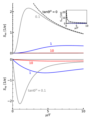
FIG. 1: Longitudinal (top) and transverse (bottom) Seebeck coefficients for varying chemical potential and $\tan\Theta^{\textrm{H}}=\sigma_{xy}/\sigma_{xx}^{\infty}$ values. Inset: zoomed out view of the longitudinal Seebeck coefficient. For $\tan\Theta^{\textrm{H}}=0$, $S_{xx}\simeq\sqrt{\sigma_{xx}^{\infty}/\sigma_{xx}^{\textrm{diss.}}}/e\sim 1/\sqrt{T}$ near the neutrality point.

III.2 Longitudinal heat conductivity

Next, we analyze the result for the longitudinal heat conductivity, Eq. (34). In the Dirac fluid regime, the entropy terms dominate the heat conductivity and we find

$$\kappa_{xx}(\left|\mu/T\right|\ll 1)=\frac{T}{e^{2}}\left(\frac{s}{n}\right)^{2}\sigma_{xx}^{\textrm{ideal}}\left[1-\rho_{xx}\sigma_{xx}^{\textrm{ideal}}\right].$$ (37)

The most efficient energy transport is via the momentum density zero-mode. At the charge neutrality point, this mode transports energy but no electric current. The electron-electron collisions are unable to relax the energy current, and the heat conductivity behaves similarly as in a non-interacting system with the same disorder. In the limit $\mu/T\rightarrow 0$ we find the value $\kappa_{xx}\rightarrow\frac{343\pi^{2}}{2325}\frac{T}{e^{2}}\sigma_{xx}^{\infty}$, similar to the result in 2D graphene [14]. This can be written by a Drude-like formula,

$$\kappa_{xx}(\mu/T=0)=c_{v}\frac{v_{F}^{2}\bar{\tau}_{\parallel}^{\textrm{el}}}{3},$$ (38)

with $c_{v}=T\partial s/\partial T$ being the heat capacity per volume. We note that in the model of short-ranged disorder, the electron-electron collisions do affect $\kappa_{xx}(\mu/T=0)$ indirectly by modifying the effective elastic scattering time. Due to the e-e collisions, the elastic scattering rate $1/\tau_{\parallel}^{\textrm{el}}(\epsilon)$ is averaged over an energy window with the width of the temperature, causing $\kappa_{xx}(\mu/T=0)$ to be larger by a numerical factor ($\approx 30$) compared to the non-interacting result (see Appendix B). More dramatically, as the electron-electron collisions cause $\sigma_{xx}$ to be governed by the smaller time scale $\tau^{\textrm{e-e}}$, they greatly enhance the Lorenz ratio $\mathcal{L}_{xx}\equiv\kappa_{xx}/\left(T\sigma_{xx}\right)$ [which for non-interacting electrons is given by $\mathcal{L}_{0}=\pi^{2}/\left(3e^{2}\right)$] near the charge neutrality point. At the charge neutrality point, the Lorenz ratio is given by

$$\mathcal{L}_{xx}(\mu/T=0)=\frac{7\pi^{2}}{5e^{2}}\frac{\bar{\tau}_{\parallel}^{\textrm{el}}}{\tau^{\textrm{e-e}}}.$$ (39)

At charge neutrality, the longitudinal heat conductivity is unaffected by the AHE. This differs when the chemical potential is increased. Then, the momentum density zero-mode begins to carry also particle current as well as energy current, ultimately rendering it unable to transfer heat without convection. This corresponds to a cancellation by the longitudinal Seebeck response $S_{xx}$, which is the second term in Eq. (37). However, a finite Hall conductivity decreases $S_{xx}$ and thus broadens the range in which $\kappa_{xx}$ is not small, as can be seen in Fig. 2. In the limit of $\sigma_{xy}\gg\sigma_{xx}^{\infty}$, this leads to a second peak in $\kappa_{xx}$ at the region between the Dirac fluid and Fermi liquid regimes, which is slightly higher than the value at the charge neutrality point, $\kappa_{xx}(\left|\mu/T\right|\approx 2.93)\approx 1.467\frac{T}{e^{2}}\sigma_{xx}^{\infty}$.

Eventually, for $\left|\mu/T\right|\gg 1$ (we remind that throughout this work, we limit ourselves to being far from the Lifshitz transition, $\left|\mu\right|\ll v_{F}\Delta_{k}$) the thermal conductivity becomes dominated by the dissipative part of the current, decaying to $\kappa_{xx}(\left|\mu/T\right|\gg 1)=\frac{\mu}{e^{2}}\frac{\mu}{T}\sigma_{xx}^{\textrm{diss.}}$. This can be written as

$$\kappa_{xx}(\left|\mu/T\right|\gg 1)=c_{v}\frac{v_{F}^{2}\tau^{\textrm{e-e}}}{3}.$$ (40)

This gives a parameterically small Lorenz ratio,

$$\mathcal{L}_{xx}=\mathcal{L}_{0}\frac{\tau^{\textrm{e-e}}}{\bar{\tau}_{\parallel}^{\textrm{el}}},$$ (41)

reflecting that charge and thermal transport are limited by two different scattering rates [52]. Suppression of the Lorenz ratio has been observed in ultra-clean samples of WP₂ and Sb [6, 7, 9], both materials being in the degenerate regime. Nonetheless, this suppression does not necessarily arise from the materials being in the hydrodynamic regime; see Appendix C for further discussion.

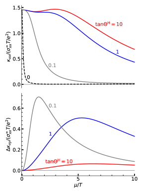
FIG. 2: Longitudinal heat conductivity $\kappa_{xx}$ (top) and deviation of the transverse heat conductivity from the WF value $\Delta\kappa_{xy}\equiv\kappa_{xy}-\mathcal{L}_{0}T\sigma_{xy}$ (bottom), for varying chemical potential and $\tan\Theta^{\textrm{H}}=\sigma_{xy}/\sigma_{xx}^{\infty}$ values.

III.3 Transverse heat conductivity

We now turn to analyze the transverse heat conductivity, Eq. (35). Keeping the leading terms we find

$$\kappa_{xy}=\frac{\pi^{2}T}{3e^{2}}\sigma_{xy}-\frac{Ts}{en}\sigma_{xx}^{\textrm{ideal}}S_{xy}.$$ (42)

The first term corresponds to the Wiedemann-Franz result in the non-interacting regime, for which the Lorenz ratio is $\mathcal{L}_{xy}=\mathcal{L}_{0}$. The second term accounts for heat transfer by the momentum density zero-mode, which acquires a transverse component due to the transverse Seebeck response. Following the behavior of the transverse Seebeck coefficient $S_{xy}$, this additional term $\Delta\kappa_{xy}\equiv\kappa_{xy}-\mathcal{L}_{0}T\sigma_{xy}$ is appreciable for small Hall-to-longitudinal conductivity ratios $\sigma_{xy}^{\textrm{}}/\sigma_{xx}^{\infty}$ (Fig. 2, bottom). In the limit $\sigma_{xy}^{\textrm{}}/\sigma_{xx}^{\infty}\ll 1$ (but $\sigma_{xy}^{\textrm{}}\gg\sigma_{xx}^{\textrm{diss.}}$), the deviation from Wiedemann-Franz law $\Delta\kappa_{xy}$ reaches a maximum

$$\left(\Delta\kappa_{xy}\right)_{\textrm{max}}\underset{\left[\sigma_{xy}^{\textrm{}}/\sigma_{xx}^{\infty}\ll 1\right]}{=}\frac{343\pi^{2}}{4650}\frac{T}{e^{2}}\sigma_{xx}^{\infty},$$ (43)

which occurs at the carrier density for which $\sigma_{xx}^{\textrm{ideal}}=\sigma_{xy}^{\textrm{}}$. Note that this peak is much higher than $\kappa_{xy}(\mu/T=0)$ in this limit, leading to a large Lorenz ratio $\mathcal{L}_{xy}=\kappa_{xy}/\left(T\sigma_{xy}\right)\simeq\mathcal{L}_{0}\sigma_{xx}^{\infty}/\sigma_{xy}$. For large $\sigma_{xy}/\sigma_{xx}^{\infty}$ ratios, the transverse Seebeck response is suppressed, and deviation from the Wiedemann-Franz law reaches a maximal value of

$$\Delta\kappa_{xy}(\left|\mu/T\right|\approx 6.34)\underset{\left[\sigma_{xy}^{\textrm{}}/\sigma_{xx}^{\infty}\gg 1\right]}{=}0.654\frac{T}{e^{2}}\frac{\left(\sigma_{xx}^{\infty}\right)^{2}}{\sigma_{xy}^{\textrm{}}}.$$ (44)

Going further into the Fermi liquid regime $\left|\mu/T\right|\gg 1$, the transverse Seebeck response diminishes and the transverse thermal conductivity decays back to the non-interacting Wiedemann-Franz result.

IV Conclusions and outlook

We considered a pair of TRS-breaking Weyl nodes with strong electron-electron scattering. We derived the hydrodynamic equations and computed the thermoelectric response coefficients. The electric and thermal currents are carried via three mechanisms: long-lived hydrodynamic zero-mode limited by disorder, dissipative modes relaxed by electron-electron collisions, and transverse transport due to the Berry curvature and magnetization currents.

We computed the effect of time-reversal symmetry breaking on the Seebeck response and heat conductivities. The anomalous Hall conductivity suppresses the longitudinal Seebeck response, which otherwise reaches the hydrodynamic limit of entropy per electric charge, but enables a transverse Seebeck response. The transverse Seebeck response is maximal when the anomalous Hall conductivity is of intermediate strength, smaller than the non-interacting limit of the longitudinal conductivity $\sigma_{xx}^{\infty}$, but larger than the electron-electron collisions limited conductivity $\sigma_{xx}^{\textrm{diss.}}$.

Due to its effect on the Seebeck response, the anomalous Hall conductivity enhances the longitudinal thermal conductivity $\kappa_{xx}$. In the TRS case, the longitudinal heat conductivity in the limiting cases $\left|\mu/T\right|\ll 1$ and $\left|\mu/T\right|\gg 1$ can be written with a Drude-like formula, $\kappa_{xx}=c_{v}v_{F}^{2}\tau/3$, with $\tau=\bar{\tau}_{\parallel}^{\textrm{el}}$ for $\left|\mu/T\right|\ll 1$ and $\tau=\tau^{\textrm{e-e}}$ for $\left|\mu/T\right|\gg 1$, describing heat transport via the momentum density zero-mode and dissipative modes, respectively. Breaking TRS, the anomalous Hall conductivity enables the longer lived zero-mode to conduct heat up until the range of $\left|\mu/T\right|\sim 1$, enhancing $\kappa_{xx}$.

The transverse heat conductivity $\kappa_{xy}$ behaves according to the Wiedemann-Franz law at the charge neutrality point. Away from the neutrality point the Wiedemann-Franz law is violated due to the large Seebeck effect. This violation is maximal for intermediate TRS-breaking, where the anomalous Hall conductivity $\sigma_{xy}$ is between the two limits of the longitudinal conductivity, $\sigma_{xx}^{\textrm{diss.}}$ and $\sigma_{xx}^{\infty}$.

In our work we assumed $\tau^{\textrm{e-e}}$ to be the shortest scattering rate in the system. This imposes a specific temperature window, where electron-phonon scattering can be neglected, as well as requiring sufficient purity of the sample. Although this parameter range is plausible, in current experiments a clear separation of scales is not yet fully achieved. In Appendix C we briefly review the typical scales for scattering mechanisms in materials that are in (or close to) the hydrodynamic regime. In this work we focused on TRS-breaking WSMs. These materials are typically more disordered, and experimental realizations do not yet reach the required purity for hydrodynamics. A viable path towards the hydrodynamic regime in TRS-breaking WSMs is likely to be via thin films. Such films have been produced recently and have less disorder and consequently smaller residual resistivity compared to bulk samples [53].

Finally, we compare the heat transport in a TRS-breaking WSM with that of a relativistic fluid in an external magnetic field [29, 30, 31] and stress the main differences. The anomalous Hall currents which flow in a WSM are additive to the hydrodynamic flow, and do not affect the longitudinal electric and thermoelectric responses. This is in contrast to the case of a magnetic field, which rotates the boost velocity, lowering the longitudinal thermoelectric conductivities $L_{xx}^{ij}$ while giving rise to ideal contributions to the transverse conductivities $L_{xy}^{ij}$. This difference has several implications.

The longitudinal thermal conductivity $\kappa_{xx}$ in a WSM is enhanced with the increase of the anomalous Hall conductivity $\sigma_{xy}$. Conversely, an external magnetic field can only decrease the longitudinal thermal conductivity. The transverse Lorenz ratio in WSM in the regime of intermediate AHE strength, $\sigma_{xx}^{\textrm{diss.}}\ll\sigma_{xy}\ll\sigma_{xx}^{\infty}$, reaches a maximum of $\mathcal{L}_{xy}\sim\sigma_{xx}^{\infty}/\sigma_{xy}$. For graphene in a weak magnetic field, the transverse Lorenz ratio can reach a maximum of $\mathcal{L}_{xy}\sim\bar{\tau}_{\parallel}^{\textrm{el}}/\tau^{\textrm{e-e}}$. As we see, the transverse Lorenz ratios at the maxima in these two systems are parametrically different.

We end this section with a brief discussion of future directions. In this work, we have limited our study to a WSM in the vicinity of the neutrality point. As one deviates from the neutrality point, the Dirac cones acquire curvature and the roles played by the various zero-modes change. In addition, a finite Fermi surface contribution to the transverse thermoelectric response coefficients $L_{xy}^{ij}$ appears. In particular, electron-electron scattering induces side jumps and skew scattering [41, 42], similar to the disorder-induced processes which contribute to the non-interacting anomalous Hall conductivity [37, 38]. It is interesting to see how such processes affect thermoelectric transport in the hydrodynamic regime. We plan to address these questions in future work.

Appendix A Derivation of the Euler equation

Here we present a derivation of the hydrodynamic equations for linearly dispersing Weyl nodes, leading to the Euler equation. Starting from the Boltzmann equation [Eq. (3)], one derives conservation equations by multiplying by conserved quantities of the electron-electron collision integral and integrating over all states. Here, these conserved quantities are the number, momentum and energy densities. In this three-mode treatment, we are summing over both Weyl nodes, utilizing our assumption that the nodes are related by inversion symmetry. Multiplying the Boltzmann equation by the corresponding charges $\lambda_{l\mathbf{k}}^{c}\in\left\{1,\mathbf{k},\epsilon_{l\mathbf{k}}\right\}$ and integrating over all states, we find

$$\frac{\partial n}{\partial t}+\mathbf{\nabla}_{r}\cdot\mathbf{J}^{n} =0,$$ (45)

$$\frac{\partial\pi^{i}}{\partial t}+\frac{\partial\Pi_{E}^{ij}}{\partial r^{j}}-eE^{i}n =\sum_{l}\intop\left(d^{3}k\right)k^{i}I_{\mathrm{imp}}\left[f_{l}(t,\mathbf{r},\mathbf{k})\right],$$ (46)

$$\frac{\partial n_{E}}{\partial t}+\mathbf{\nabla}_{r}\cdot\mathbf{J}^{E}-e\mathbf{E}\cdot\mathbf{J}^{n} =0,$$ (47)

where the number, momentum and energy densities $n^{c}\in\left\{n,\mathbf{\pi},n_{E}\right\}$ are given by

$$n^{c}(\mathbf{r},t)=\sum_{l}\intop\left(d^{3}k\right)\lambda_{l\mathbf{k}}^{c}f_{l\mathbf{k}}(\mathbf{r},t),$$ (48)

$\Pi_{E}^{ij}=\sum_{l}\intop\left(d^{3}k\right)k^{i}v_{l\mathbf{k}}^{j}f_{l\mathbf{k}}$ is the momentum-flux tensor and $\mathbf{J}^{n},\mathbf{J}^{E}$ are the particle and energy currents. The densities $n,\mathbf{\pi},n_{\epsilon}$ correspond to their conjugate potentials (chemical potential, boost velocity and temperature) which parametrize the zero-mode distribution function. In the equation for momentum conservation, Eq. (46), we assumed equal chemical potential for pairing Weyl nodes, due to the absence of a magnetic field. If we relax this assumption and introduce chiral charge, Eq. (46) acquires a term due originating from the anomalous velocity [23].

Calculation of the momentum density, energy current density and momentum-flux tensor yields

$$\mathbf{\pi} =\frac{w}{v_{F}^{2}}\mathbf{u},$$ (49)

$$\mathbf{J}^{E} =w\mathbf{u},$$ (50)

$$\Pi_{E}^{ij} =p\delta^{ij}+w\frac{u^{i}u^{j}}{v_{F}^{2}}+\delta\Pi_{E}^{ij}.$$ (51)

Here, $p$ is the pressure and $w=n_{\epsilon}+p$ is the enthalpy density. $\delta\Pi_{E}^{ij}$ is a dissipative correction to the momentum-flux tensor which corresponds to viscosity, and is proportional to the gradients of $\mathbf{u}$ [28]. It will not be important for transport in a macroscopic sample [14]. The energy current density is proportional to the momentum density $\mathbf{J}^{E}=v_{F}^{2}\mathbf{\pi}$ due to the linear dispersion relation of the WSM. Substituting the above expressions in Eq. (46), using the energy conservation Eq. (47) and neglecting viscosity, we obtain the Euler equation

$$w\left(\frac{\partial}{\partial t}+\mathbf{u}\cdot\mathbf{\nabla}_{r}\right)\mathbf{u}+v_{F}^{2}\mathbf{\nabla}_{r}p+\mathbf{u}\frac{\partial p}{\partial t}-v_{F}^{2}en\mathbf{E}$$

$$+e\left(\mathbf{E}\cdot\mathbf{J}^{n}\right)\mathbf{u}$$

$$=\sum_{l}\intop\left(d^{3}k\right)\mathbf{k}I_{\mathrm{e-imp}}\left[f_{l}(t,\mathbf{r},\mathbf{k})\right].$$ (52)

The RHS describes momentum relaxation by disordered impurities, and it is given by

$$\sum_{l}\intop\left(d^{3}k\right)\mathbf{k}I_{\mathrm{e-imp}}\left[f_{l}(t,\mathbf{r},\mathbf{k})\right]=-\frac{\mathbf{u}}{\bar{\tau}_{\parallel}^{\textrm{el}}}\frac{w}{v_{F}^{2}},$$ (53)

where the effective elastic transport time $\bar{\tau}_{\parallel}^{\textrm{el}}$ is calculated in the next section. Finally, using the thermodynamic relation $dp=nd\mu+sdT$ we obtain the form of the Euler equation written in the main text, Eq. (6). For the calculation of DC conductivities done in the main text, the time derivative term is set to zero. We then find the boost velocity, to linear order in the fields, to be given by

$$\mathbf{u}=\frac{v_{F}^{2}\bar{\tau}_{\textrm{{\hbox{\parallel}}}}^{\textrm{el}}}{w}\left[n\left(e\mathbf{E}+\mathbf{\nabla}_{r}\mu\right)-s\mathbf{\nabla}_{r}T\right].$$ (54)

We note that here, the boost velocity is limited only by the disorder. In a different setup, the boost velocity may be limited by other scales, such as a finite frequency of the fields. In this case one should replace $\bar{\tau}_{\parallel}^{\textrm{el}}\rightarrow\bar{\tau}_{\parallel}^{\textrm{el}}/\left(1-i\omega\bar{\tau}_{\parallel}^{\textrm{el}}\right)$ in the above equation. If the sample size is smaller than the elastic transport length, it should be used as a cut-off for the momentum density zero-mode.

Appendix B Elastic transport scattering time

The disorder collision integral is given by (omitting node and band indices as the scattering is elastic and we assumed no internode scattering by the disorder )

$$I_{\mathrm{e-imp}}\left[f_{\mathbf{k}}\right]=-\intop\left(d^{3}k^{\prime}\right)\left(f_{\mathbf{k}}-f_{\mathbf{k}^{\prime}}\right)w_{\mathbf{k}\mathbf{k}^{\prime}},$$ (55)

Where $w_{\mathbf{k}\mathbf{k}^{\prime}}=2\pi\left|V_{\mathbf{k}\mathbf{k}^{\prime}}\right|^{2}\delta(\epsilon_{\mathbf{k}}-\epsilon_{\mathbf{k}^{\prime}})$ is the scattering rate, given by Fermi’s golden rule. The elastic transport time at a given energy is given by taking $f_{\mathbf{k}}\propto\hat{k}$,

$$\frac{\hat{k}}{\tau_{\parallel}^{\textrm{el}}(\epsilon)}=-\intop\left(d^{3}k^{\prime}\right)\left(\hat{k}-\hat{k}^{\prime}\right)w_{\mathbf{k}\mathbf{k}^{\prime}}=\frac{2\pi\gamma\nu(\epsilon)}{3}\hat{k},$$ (56)

where $\nu(\epsilon)$ is the density of states of the single Weyl node at energy $\epsilon$ and $\gamma$ is the amplitude of the short-ranged disorder potential correlator [Eq. (2)]. Note that due to the spinor structure, low-angle scattering is favored (The matrix element $V_{\mathbf{k}\mathbf{k}^{\prime}}$ contains the product of the Bloch eigenfunctions at $\mathbf{k},\mathbf{k}^{\prime}$), making the transport time larger than the elastic lifetime by a factor of $3/2$.

In the derivation of the Euler equation [Eq. (52)], the elastic transport rate $1/\tau_{\parallel}^{\textrm{el}}(\epsilon)$ is thermally averaged:

$$\sum_{l}\intop\left(d^{3}k\right)\mathbf{k}I_{\mathrm{e-imp}}\left[f_{l}(t,\mathbf{r},\mathbf{k})\right]=-\mathbf{u}\sum_{l}\intop\left(d^{3}k\right)\left(-\frac{\partial f^{0}(\epsilon_{l\mathbf{k}})}{\partial\epsilon}\right)\frac{k^{2}}{3\tau_{\parallel}^{\textrm{el}}(\epsilon_{l\mathbf{k}})},$$ (57)

where we linearized $f$ in the boost velocity, $f\approx f_{0}-\frac{\partial f_{0}}{\partial\epsilon}\mathbf{u}\cdot\mathbf{k}$. We write the above expression by defining a thermally averaged transport rate $1/\bar{\tau}_{\parallel}^{\textrm{el}}$:

$$\sum_{l}\intop\left(d^{3}k\right)\mathbf{k}I_{\mathrm{e-imp}}\left[f_{l}(t,\mathbf{r},\mathbf{k})\right]=-\frac{\mathbf{u}}{\bar{\tau}_{\parallel}^{\textrm{el}}}\sum_{l}\intop\left(d^{3}k\right)\left(-\frac{\partial f^{0}(\epsilon_{l\mathbf{k}})}{\partial\epsilon}\right)\frac{k^{2}}{3}=-\frac{\mathbf{u}}{\bar{\tau}_{\parallel}^{\textrm{el}}}\frac{w}{v_{F}^{2}},$$ (58)

where the averaged transport rate can be seen to be given by

$$\frac{1}{\bar{\tau}_{\parallel}^{\textrm{el}}}=\frac{\sum_{l}\intop\left(d^{3}k\right)\left(-\frac{\partial f^{0}(\epsilon_{l\mathbf{k}})}{\partial\epsilon}\right)\frac{k^{2}}{\tau_{\parallel}^{\textrm{el}}(\epsilon_{l\mathbf{k}})}}{\sum_{l}\intop\left(d^{3}k\right)\left(-\frac{\partial f^{0}(\epsilon_{l\mathbf{k}})}{\partial\epsilon}\right)k^{2}}.$$ (59)

Explicit calculation yields

$$\frac{1}{\bar{\tau}_{\parallel}^{\textrm{el}}}=\frac{1}{\tau_{\parallel}^{\textrm{el}}(\epsilon=T)}\frac{\left(\beta\mu\right)^{6}+5\pi^{2}\left(\beta\mu\right)^{4}+7\pi^{4}\left(\beta\mu\right)^{2}+\frac{31\pi^{6}}{21}}{\left(\beta\mu\right)^{4}+2\pi^{2}\left(\beta\mu\right)^{2}+\frac{7\pi^{4}}{15}}\approx\begin{cases}\frac{155\pi^{2}}{49}1/\tau_{\parallel}^{\textrm{el}}(\epsilon=T)&\mu\ll T,\\ 1/\tau_{\parallel}^{\textrm{el}}(\epsilon=\mu)&\mu\gg T.\end{cases}$$ (60)

Interestingly, for low temperatures $\left(\bar{\tau}_{\parallel}^{\textrm{el}}\right)^{-1}$ is greatly enhanced (factor of $\sim 30$) compared to the naive estimation $\left(\bar{\tau}_{\parallel}^{\textrm{el}}\right)^{-1}\approx\left(\tau_{\parallel}^{\textrm{el}}(\epsilon=T)\right)^{-1}$; the high-energy electrons, which scatter faster, are given a higher weight in the momentum relaxation integral.

Appendix C Experimental realizations of electron hydrodynamics in semimetals

Here we review some experimental properties of semimetals exhibiting (or being close to) the hydrodynamic regime. In particular, we discuss the scales of the different scattering mechanisms and their compatibility with our simple model, which neglects electron-phonon scattering and assumes electron-electron scattering time to be the shortest.

Signatures of the hydrodynamic regime have been reported in the type-II, time-reversal symmetric WSM WP₂ [6, 7], and in the closely related but non-Weyl phase of WTe₂ [8, 10]. We summarize the values of scattering lengths based on recent experiments and ab initio calculations in Table 1.

It is worth mentioning that ab initio calculations [55, 8] for both materials show that the bare Coulomb interaction is strongly screened by the free carriers. The effective electron-electron interaction emerges due to the exchange of virtual phonons. We emphasize that this virtual phonon-mediated interaction strictly conserves the energy and momentum of the electronic system, as opposed to a real phonon absorption/emission process (the latter corresponds to $\ell^{\textrm{e-ph}}$ in Table 1). Since the microscopic origins of the electron-electron interaction are not consequential for our analysis, this mechanism still leads to hydrodynamics of the same type as we consider. The only influence of the microscopic origin of the electron-electron interaction is incorporated in the dependence of $\tau^{\textrm{e-e}}$ on the temperature and chemical potential. Such an analysis in the case of phonon-mediated electron-electron interaction has recently been done in Ref. [56].

Material	References	T [K]	$\mathbf{\ell^{\textrm{e-e}}[\mu m]}$	$\mathbf{\ell^{\textrm{e-ph}}[\mu m]}$	$\mathbf{\ell^{\textrm{e-imp}}[\mu m]}$
WTe2	Experimental realizations in Refs. [8, 10], ab initio calculations in Ref. [8] [*]	5	25	150	1.8
		10	2.5	7.5
		15	1	2
		50	0.1	0.1
WP2	Experimental realizations in Refs. [6, 7], ab initio calculations in Ref. [55]	5	200	30	100 [6]
		10	9	5
		15	1.5	1.5
		50	0.03	0.04
Sb	Experimental and fitted parameters from Ref. [9]	3.5	1000	[**]	200 (cleanest sample)
		7.5	300

Table 1: Scattering lengths for different materials, collected from other works. Data from Ref. [8] are ab initio calculations taken from Fig. 4. Data from Ref. [55] are taken from Fig. 2, with $v_{F}=1.4\cdot 10^{5}m/s$ to convert from scattering times to lengths. For Sb, the lengths $\ell^{\textrm{e-e}}$ are the Principi-Vignale formula fitted values of Fig. 6 in Ref. [9]. In both calculations for WP₂ and WTe₂, the dominant electron-electron scattering is due to the phonon-mediated interaction.
[*] Calculations in Ref. [10] suggest that $\ell^{\textrm{e-e}}$ in WTe₂ may be smaller due to enhanced Coulomb scattering.
[**] Ref. [9] argues negligible e-ph in Sb at the measured temperatures. The argument is expecting a Bloch-Grüneisen contribution to the resistivity of $\rho_{\textrm{BG}}\sim T^{5}$ from phonons, while the data shows a negligible $\sim T^{5}$ term compared to the constant and $\sim T^{2}$ parts of the resistivity.

By analyzing the experimental data summarized in Table 1 one concludes that though the hydrodynamic regime ($l^{\rm{e-e}}<l^{\rm{imp}}<l^{{\rm e-ph}}$) can be achieved, the separation between the scattering scales is not large. Therefore the majority of experiments up to date are on the verge of the formation of the hydrodynamic regime. Both electron-impurity and electron-phonon scattering can mask the hydrodynamic effects.

Among the effects that fit into the hydrodynamic picture are the experiments in WP₂ that have reported a low Lorentz ratio [6, 7], in agreement with the hydrodynamic result [Eq. (41)] at the degenerate regime ($\left|\mu/T\right|\gg 1$). Similar behavior has been also shown in antimony (Sb) [9]. However, in the antimony experiment, the impurity scattering length was comparable with the electron-electron scattering length. Therefore, the comparison with formula Eq. (41) should be performed using its modified form, the Principi-Vignale result, replacing $\tau^{\textrm{e-e}}/\bar{\tau}_{\parallel}^{\textrm{el}}\rightarrow\tau^{\textrm{e-e}}/\left(\tau^{\textrm{e-e}}+\bar{\tau}_{\parallel}^{\textrm{el}}\right)$ [52].

It should be noted that a low Lorenz ratio can also result from other mechanisms. Particularly, due to different relaxation rates for the electric and energy currents [7]. Small-angle inelastic momentum-relaxing scattering (i.e. electron-phonon or Umklapp electron-electron) relaxes the energy current much faster than the electric current (in the degenerate regime, where the electric current is nearly equivalent to the total momentum [52]).

It is worth mentioning that electron-electron Umklapp scattering mechanism may be relevant for WP₂. This is due to electron and hole Fermi pockets separated in momentum space, enhancing electron-electron Umklapp scattering [7]. In this case, one has to distinguish between the normal (momentum-conserving) and Umklapp (momentum-relaxing) electron-electron scattering rates. In our model, $\tau^{\textrm{e-e}}$ denotes only the normal part of the e-e collisions. Significant Umklapp scatterings would contribute to the relaxation of the momentum density as well as the electric and heat currents.

It is also worth to mention that the dominant mechanism of phonon decay over a wide temperature range in WP₂ is via phonon-electron scattering, rather than phonon-phonon scattering[57]. This implies that the electron and phonon degrees of freedom in this material are strongly coupled. In this case, the energy and momentum of the coupled electron-phonon fluid are conserved [57, 58]. This regime is outside the scope of our work.

Appendix D Thermodynamic quantities

Here we present some results for thermodynamics quantities for an isolated Weyl node with 3D linear spectrum $H=v_{F}\mathbf{\sigma}\cdot\mathbf{k}$.

The grand potential of the system is given by [59]

$$\Omega(T,V,\mu) =-\frac{1}{\beta}\sum_{b}\prod_{\mathbf{k}}\left[1+\exp\left(\beta\left(\mu-\epsilon_{b\mathbf{k}}\right)\right)\right]=-\frac{1}{\beta}\sum_{b\mathbf{k}}\ln\left[1+\exp\left(\beta\left(\mu-\epsilon_{b\mathbf{k}}\right)\right)\right]$$

$$=\frac{V}{\pi^{2}\beta^{4}v_{F}^{3}}\left[\mathrm{Li}_{4}(-e^{\beta\mu})+\mathrm{Li}_{4}(-e^{-\beta\mu})\right],$$ (61)

where

$$\mathrm{Li}_{s}(-z)=-\frac{1}{\left(s-1\right)!}\intop_{0}^{\infty}\frac{t^{s-1}}{z^{-1}e^{t}+1}dt$$ (62)

is the polylogarithm function. From the grand potential one can derive the thermodynamic quantities:

$$p =-\frac{\Omega}{V},$$ (63)

$$N =-\frac{\partial\Omega}{\partial\mu}=-\frac{V}{\pi^{2}\beta^{3}v_{F}^{3}}\left[\mathrm{Li}_{3}(-e^{\beta\mu})-\mathrm{Li}_{3}(-e^{-\beta\mu})\right],$$ (64)

$$S =-\frac{\partial\Omega}{\partial T}=\beta\left(4pV-\mu N\right).$$ (65)

In terms of densities we find

$$w =\frac{1}{6\pi^{2}\beta^{4}v_{F}^{3}}\left[\left(\beta\mu\right)^{4}+2\pi^{2}\left(\beta\mu\right)^{2}+\frac{7\pi^{4}}{15}\right],$$ (66)

$$s =\frac{1}{6\beta^{3}v_{F}^{3}}\left[\left(\beta\mu\right)^{2}+\frac{7\pi^{2}}{15}\right],$$ (67)

$$n =\frac{1}{6\pi^{2}\beta^{3}v_{F}^{3}}\beta\mu\left[\left(\beta\mu\right)^{2}+\pi^{2}\right].$$ (68)

In the system we consider, assuming $\left|\mu\right|,T\ll\left(\Delta_{k}v_{F}\right)$, we extend the momentum integration for each Weyl node to infinity and get that the extensive quantities are simply the above results multiplied by the number of nodes $N_{W}=2$. However, there is a subtlety here if the boost velocity is finite. Since the boost velocity $\mathbf{u}$ of the whole system couples to the quasimomentum $\mathbf{k}$, one has to consistently choose the same origin in k-space for both nodes. This effectively leads to the two nodes equilibrating to different chemical potentials, $\mu_{\eta}=\mu+\eta\mathbf{u}\cdot\mathbf{\Delta}_{k}/2$. Therefore, an external field along the node separation axis causes a charge drift between the nodes. For the quantities we consider, the effect can be disregarded on the linear response level.

The density of states of a single Weyl node is given by

$$\nu(\epsilon)=\frac{\epsilon^{2}}{2\pi^{2}v_{F}^{3}}.$$ (69)

In the above calculations, we used the following useful identities for the polylogarithms functions [60]:

$$\mathrm{Li}_{2}(-e^{x})+\mathrm{Li}_{2}(-e^{-x}) =-\frac{x^{2}}{2}-\frac{\pi^{2}}{6},$$ (70)

$$\mathrm{Li}_{3}(-e^{x})-\mathrm{Li}_{3}(-e^{-x}) =-\frac{x^{3}}{6}-\frac{\pi^{2}}{6}x,$$ (71)

$$\mathrm{Li}_{4}(-e^{x})+\mathrm{Li}_{4}(-e^{-x}) =-\frac{1}{24}x^{4}-\frac{\pi^{2}}{12}x^{2}-\frac{7\pi^{4}}{360},$$ (72)

$$\mathrm{Li}_{6}(-e^{x})+\mathrm{Li}_{6}(-e^{-x}) =-\frac{1}{6!}\left(x^{6}+5\pi^{2}x^{4}+7\pi^{4}x^{2}+\frac{31\pi^{6}}{21}\right).$$ (73)

Appendix E Calculation of dissipative linear response coefficients

In this part, we calculate the dissipative response coefficients by approximately solving the electron-electron collision integral. To the leading order in $\bar{\tau}_{\parallel}^{\textrm{el}}/\tau^{\textrm{e-e}}$, the disorder collision integral can be neglected, and from hereon we take $I\left[f\right]\approx I_{\textrm{e-e}}\left[f\right]$.

We write the distribution function as $f=f^{\textrm{FD}}+\delta f$, where $f^{\textrm{FD}}$ is a local equilibrium Fermi-Dirac distribution and $\delta f$ is the non-equilibrium dissipative correction. Let us parametrize this correction by

$$\delta f_{l}(\mathbf{k})=g(\epsilon_{l\mathbf{k}})h_{l}(\mathbf{k}),$$ (74)

where $h(\mathbf{k})$ is any function and

$$g(\epsilon)=\sqrt{-\frac{1}{\beta}\frac{\partial f^{0}}{\partial\epsilon}}=\frac{1}{2\cosh\left(\frac{\epsilon-\mu}{2T}\right)}.$$ (75)

The linearized Boltzmann equation reads

$$-\beta g^{2}(\epsilon_{l\mathbf{k}})\left[\mathbf{v}_{l\mathbf{k}}\cdot\left(e\mathbf{E}-\mathbf{\nabla}\mu\right)-\frac{\mathbf{v}_{l\mathbf{k}}\left(\epsilon_{l\mathbf{k}}-\mu\right)}{T}\cdot\mathbf{\nabla}T\right]=I\left[\delta f_{l}(\mathbf{k})\right].$$ (76)

In order to solve the Boltzmann equation, one has to invert the collision integral. However, the e-e collision integral has zero-modes, and so first we must project the Boltzmann equation to the subspace orthogonal to these zero-modes. The zero-modes correspond to the conserved quantities of the collision integral: charge, momentum and energy densities, and are given by

$$\lambda_{l}^{(1)}(\mathbf{k})=1,\qquad\lambda_{l}^{(2)}(\mathbf{k})=\mathbf{k},\qquad\lambda_{l}^{(3)}(\mathbf{k})=\epsilon_{l\mathbf{k}}.$$ (77)

We linearize the collision integral, and define the inner product space

$$\left\langle\psi|\phi\right\rangle\equiv\sum_{l}\intop\left(d\mathbf{k}\right)\psi_{l}(\mathbf{k})g^{2}(\epsilon_{l\mathbf{k}})\phi_{l}(\mathbf{k}).$$ (78)

We symmetrize the collision integral in this inner product space by defining

$$\mathscr{\mathcal{I}}_{l\mathbf{k},l^{\prime}\mathbf{k}^{\prime}}\equiv\frac{1}{g(\epsilon_{l\mathbf{k}})}I_{l\mathbf{k},l^{\prime}\mathbf{k}^{\prime}}g(\epsilon_{l^{\prime}\mathbf{k}^{\prime}}).$$ (79)

Substituting the symmetrized collision operator in the Boltzmann equation, we can invert it in the subspace orthogonal to the zero-modes and find

$$h_{l}(\mathbf{k})=-\beta\sum_{l^{\prime}}\intop\left(d\mathbf{k}^{\prime}\right)\mathscr{\mathcal{I}}_{l\mathbf{k},l^{\prime}\mathbf{k}^{\prime}}^{-1}g(\epsilon_{l^{\prime}\mathbf{k^{\prime}}})\left[\mathbf{v}_{l^{\prime}\mathbf{k}^{\prime}}\cdot\left(e\mathbf{E}-\mathbf{\nabla}\mu\right)-\frac{\mathbf{v}_{l^{\prime}\mathbf{k}^{\prime}}\left(\epsilon_{l^{\prime}\mathbf{k}^{\prime}}-\mu\right)}{T}\mathbf{\nabla}T\right].$$ (80)

At this stage, we approximate the inverse e-e collision integral to be simply given by $\mathscr{\mathcal{I}}_{l\mathbf{k},l^{\prime}\mathbf{k}^{\prime}}^{-1}=-\tau^{\textrm{e-e}}\delta\left(\mathbf{k}-\mathbf{k}^{\prime}\right)\delta_{ll^{\prime}}$. We then find the dissipative corrections to the currents,

$$\mathbf{J}_{\textrm{diss.}}^{i}\equiv\sum_{l}\intop\left(d\mathbf{k}\right)\mathbf{j}_{l\mathbf{k}}^{i}\delta f_{l\mathbf{k}}=\beta\tau^{\textrm{e-e}}\left\langle\mathbf{j}^{i}|\mathbf{v}\cdot\left[e\mathbf{E}-\mathbf{\nabla}\mu-\frac{\left(\epsilon-\mu\right)}{T}\mathbf{\nabla}T\right]\right\rangle,$$ (81)

where $i=1,2$ indicate the electric and thermal currents, with their operators given by

$$\mathbf{j}^{\textrm{1}}=e\mathbf{v}_{l\mathbf{k}},\qquad\qquad\qquad\mathbf{j}^{\textrm{2}}=\left(\epsilon_{l\mathbf{k}}-\mu\right)\mathbf{v}_{l\mathbf{k}}.$$ (82)

In the RHS of Eq. (81), both vectors are projected to the subspace orthogonal to the zero-modes. Eq. (81) can be written more compactly as

$$J_{\textrm{diss.,}\alpha}^{i}=L_{\textrm{diss.,}\alpha\beta}^{ij}F_{\beta}^{j},$$ (83)

where $\mathbf{F}^{i}$ are generalized forces, $L_{\textrm{diss.}}^{ij}$ are the dissipative parts of the total thermoelectric response tensors defined in the main text [Eqs. (13), (14)], and explicitly:

$$\mathbf{F}^{\textrm{1}} =\mathbf{E}-\frac{\mathbf{\nabla}\mu}{e},\qquad\qquad\qquad\mathbf{F}^{\textrm{2}}=-\mathbf{\nabla}T,$$ (84)

$$L_{\textrm{diss.,}\alpha\beta}^{ij} =-\beta\left\langle j_{\alpha}^{i}|\mathscr{\hat{\mathcal{I}}}^{-1}j_{\beta}^{j}\right\rangle.$$ (85)

By computing Eq. (85) we find,

$$L_{\textrm{diss.,}xx}^{\textrm{11}} =\sigma_{xx}^{\textrm{{diss.}}}=e^{2}v_{F}^{2}\left(\frac{1}{3}\frac{\partial n}{\partial\mu}-\frac{n^{2}}{w}\right)\tau^{\textrm{e-e}},$$ (86)

$$L_{\textrm{diss.,}xx}^{\textrm{21}} =TL_{\textrm{diss,}xx}^{\textrm{12}}=-\frac{\mu}{e}\sigma_{xx}^{\textrm{{diss.}}},$$ (87)

$$L_{\textrm{diss.,}xx}^{\textrm{22}} =\frac{\mu^{2}}{e^{2}T}\sigma_{xx}^{\textrm{diss.}}.$$ (88)

In our approximation for the electron-electron collision integral, there are no contributions to the off-diagonal dissipative response coefficients, $L_{\textrm{diss.,}xy}^{ij}=0$. Interestingly, $\sigma_{xx}^{\textrm{diss.}}$ can be written by a Drude-like formula in the two opposite limits of $\mu/T$:

$$\sigma_{xx}^{\textrm{diss.}}\approx\frac{e^{2}v_{F}^{2}}{3}\tau^{\textrm{e-e}}\times\begin{cases}\frac{\partial n}{\partial\mu}&\left|\mu/T\right|\ll 1,\\ \frac{T}{\mu^{2}}c_{v}&\left|\mu/T\right|\gg 1,\end{cases}$$ (89)

with $c_{v}=T\partial s/\partial T$ being the heat capacity. This result reflects that the momentum zero-mode is parallel to the thermal current in the Dirac fluid regime, and to the particle current in the Fermi liquid regime. Dissipation occurs via the orthogonal channels, therefore $\sigma_{xx}^{\textrm{diss.}}$ is related to particle diffusion in the Dirac fluid and heat diffusion in the Fermi liquid.

Lastly, we address the electron-electron scattering time $\tau^{\textrm{e-e}}$. In Weyl semimetals, the electron-electron scattering rate can be estimated by $1/\tau^{\textrm{e-e}}\sim N_{W}\alpha^{2}T\min\left(1,\frac{T}{\mu}\right)$ [61, 62], where $N_{W}$ is the number of Weyl nodes and $\alpha$ is the effective fine-structure constant, characterizing the ratio between the typical Coulomb interaction energy scale and the typical kinetic energy scale. The condition $\tau^{\textrm{e-e}}\ll\bar{\tau}_{\parallel}^{\textrm{el}}$ gives a condition for the maximal strength of the disorder,

$$\gamma\ll\frac{v_{F}^{3}\alpha^{2}T^{2}}{\max(\mu^{3},T^{3})}.$$ (90)

Appendix F Seebeck coefficient for non-interacting electrons

Here, we calculate the temperature dependence of the Seebeck coefficient in a non-interacting system with particle-hole symmetry. While the calculation is standard for the Fermi-liquid regime ($\mu\gg T$) [11, 50, 63], for the Dirac fluid regime ($\mu\ll T$) it is less commonly found in the literature, and so we carry it here for comparison with the hydrodynamic regime. For simplicity, we focus on an isotropical system and omit the tensor structure (in space) of the response coefficients. For non-interacting electrons, the thermoelectric response $L^{\textrm{12}}$ can be calculated from the Mott relation

$$L^{\textrm{12}}=\frac{1}{e}\intop d\epsilon\frac{\epsilon-\mu}{T}\sigma^{\textrm{}}(\epsilon)\left(-\frac{\partial f^{0}}{\partial\epsilon}\right),$$ (91)

where

$$\sigma(\epsilon)=e^{2}\intop\left(d\mathbf{k}\right)\delta(\epsilon-\epsilon_{\mathbf{k}})v^{2}(\mathbf{k})\tau(\mathbf{k})$$ (92)

is the electric conductivity at zero temperature. For an isotropic system,

$$\sigma(\epsilon)=\frac{e^{2}v_{F}^{2}(\epsilon)\nu(\epsilon)}{d}\tau(\epsilon),$$ (93)

where $d$ is the number of dimensions. One can utilize the Sommerfeld expansion

$$\intop_{-\infty}^{\infty}K(\epsilon)\left(-\frac{\partial f}{\partial\epsilon}\right)d\epsilon$$

$$=K(\mu)+\sum_{n=1}^{\infty}a_{n}\left(T\right)^{2n}\frac{d^{2n}}{d\epsilon^{2n}}K(\epsilon)|_{\epsilon=\mu},$$ (94)

where $a_{n}$ are dimensionless coefficients, the first ones given by $a_{1}=\pi^{2}/6,$ $a_{2}=7\pi^{4}/360$. Writing $v_{F}^{2}(\epsilon)\nu(\epsilon)\sim\epsilon^{\alpha}$ and $\tau\sim\epsilon^{\beta}$ (for example, in 3D metals with scattering due to short-ranged impurities, $\alpha=3/2,\beta=-1/2$) one finds for the Fermi-liquid regime, to leading order in $\epsilon_{F}/T$,

$$L^{11} =\sigma(\epsilon_{F}),$$ (95)

$$L^{12} =\frac{\pi^{2}}{3e}T\left.\frac{d\sigma}{d\epsilon}\right|_{\epsilon=\epsilon_{F}}=\frac{\pi^{2}}{3e}\frac{T}{\epsilon_{F}}\left(\alpha+\beta\right)\sigma(\epsilon_{F}),$$ (96)

leading to the Seebeck coefficient

$$S=\frac{L^{12}}{L^{11}}=\frac{\pi^{2}}{3e}\frac{T}{\epsilon_{F}}\left(\alpha+\beta\right).$$ (97)

The thermopower of WSMs in the linear dispersion regime was studied by Lundgren et al. [64]. In WSMs, $\alpha=2$. Focusing on the leading order in $\epsilon_{F}/T$, their results imply $\beta=2$ for scattering due to charged impurities and $\beta=-2$ for short-ranged impurities. Plugging these values in Eq. (97) gives agreement with Ref. [64].

In the Dirac fluid regime, one can still perform the Sommerfeld expansion as long as $\sigma(\epsilon)$ is a polynomial function of $\epsilon$. Assuming particle-hole symmetry, $\sigma(\epsilon)$ is even in energy. Denoting the highest power of $\epsilon$ in the expansion of $\sigma(\epsilon)$ as $2\gamma$, one finds, to the leading order in $T/\mu$,

$$L^{11} =a_{\gamma}\left(2\gamma\right)!\left(\frac{T}{\mu}\right)^{2\gamma}\sigma(\mu),$$ (98)

$$L^{12} =\frac{1}{e}a_{\gamma}\left(2\gamma\right)!\left(\frac{T}{\mu}\right)^{2\gamma-1}\sigma(\mu),$$ (99)

leading to

$$S=\frac{1}{e}\frac{\mu}{T}.$$ (100)

We see that the Seebeck coefficient in the non-interacting Dirac fluid regime scales as $\mu/T$, in contrast to the hydrodynamic regime where it scales as $s/n\simeq T/\mu$.

References

- Levitov and Falkovich [2016] L. Levitov and G. Falkovich, Electron viscosity, current vortices and negative nonlocal resistance in graphene, Nat. Phys. 12, 672 (2016).
- Gurzhi [1963] R. N. Gurzhi, Minimum of resistance in impurity free conductors, Sov. Phys. JETP 17, 521 (1963).
- Ghahari et al. [2016] F. Ghahari, H. Y. Xie, T. Taniguchi, K. Watanabe, M. S. Foster, and P. Kim, Enhanced thermoelectric power in graphene: Violation of the Mott relation by inelastic scattering, Phys. Rev. Lett. 116, 136802 (2016).
- Moll et al. [2016] P. J. W. Moll, P. Kushwaha, N. Nandi, B. Schmidt, and A. P. Mackenzie, Evidence for hydrodynamic electron flow in PdCoO2, Science 351, 1061 (2016).
- Crossno et al. [2016] J. Crossno, J. K. Shi, K. Wang, X. Liu, A. Harzheim, A. Lucas, S. Sachdev, P. Kim, T. Taniguchi, K. Watanabe, T. A. Ohki, and K. C. Fong, Observation of the Dirac fluid and the breakdown of the Wiedemann-Franz law in graphene, Science 351, 1058 (2016).
- Gooth et al. [2018] J. Gooth, F. Menges, N. Kumar, V. Süß, C. Shekhar, Y. Sun, U. Drechsler, R. Zierold, C. Felser, and B. Gotsmann, Thermal and electrical signatures of a hydrodynamic electron fluid in tungsten diphosphide, Nat. Commun. 9, 1 (2018).
- Jaoui et al. [2018] A. Jaoui, B. Fauqué, C. W. Rischau, A. Subedi, C. Fu, J. Gooth, N. Kumar, V. Süß, D. L. Maslov, C. Felser, and K. Behnia, Departure from the Wiedemann-Franz law in WP2 driven by mismatch in T-square resistivity prefactors, npj Quantum Mater. 3, 64 (2018).
- Vool et al. [2021] U. Vool, A. Hamo, G. Varnavides, Y. Wang, T. X. Zhou, N. Kumar, Y. Dovzhenko, Z. Qiu, C. A. Garcia, A. T. Pierce, J. Gooth, P. Anikeeva, C. Felser, P. Narang, and A. Yacoby, Imaging phonon-mediated hydrodynamic flow in WTe2, Nat. Phys. 17, 1216 (2021).
- Jaoui et al. [2021] A. Jaoui, B. Fauqué, and K. Behnia, Thermal resistivity and hydrodynamics of the degenerate electron fluid in antimony, Nat. Commun. 12, 195 (2021).
- Aharon-Steinberg et al. [2022] A. Aharon-Steinberg, T. Völkl, A. Kaplan, A. K. Pariari, I. Roy, T. Holder, Y. Wolf, A. Y. Meltzer, Y. Myasoedov, M. E. Huber, B. Yan, G. Falkovich, L. S. Levitov, M. Hücker, and E. Zeldov, Direct observation of vortices in an electron fluid, Nature 607, 74 (2022).
- Ashcroft and Mermin [1976] N. W. Ashcroft and N. D. Mermin, Solid State Physics (Holt, Rinehart and Winston, 1976).
- Fu et al. [2020] C. Fu, Y. Sun, and C. Felser, Topological thermoelectrics, APL Mater. 8, 040913 (2020).
- Andersen et al. [2019] T. I. Andersen, T. B. Smith, and A. Principi, Enhanced photoenergy harvesting and extreme Thomson effect in hydrodynamic electronic systems, Phys. Rev. Lett. 122, 166802 (2019).
- Lucas and Fong [2018] A. Lucas and K. C. Fong, Hydrodynamics of electrons in graphene, J. Phys. Condens. Matter 30, 053001 (2018).
- Yan and Felser [2017] B. Yan and C. Felser, Topological materials: Weyl semimetals, Annu. Rev. Condens. Matter Phys. 8, 337 (2017).
- Armitage et al. [2018] N. P. Armitage, E. J. Mele, and A. Vishwanath, Weyl and Dirac semimetals in three-dimensional solids, RMP 90, 015001 (2018).
- Xiao et al. [2010] D. Xiao, M. C. Chang, and Q. Niu, Berry phase effects on electronic properties, RMP 82, 1959 (2010).
- Burkov and Balents [2011] A. A. Burkov and L. Balents, Weyl semimetal in a topological insulator multilayer, Phys. Rev. Lett. 107, 127205 (2011).
- Qin et al. [2011] T. Qin, Q. Niu, and J. Shi, Energy magnetization and the thermal Hall effect, Phys. Rev. Lett. 107, 236601 (2011).
- Haldane [2004] F. D. M. Haldane, Berry curvature on the fermi surface: Anomalous hall effect as a topological fermi-liquid property, Phys. Rev. Lett. 93, 206602 (2004).
- Xiao et al. [2006] D. Xiao, Y. Yao, Z. Fang, and Q. Niu, Berry-phase effect in anomalous thermoelectric transport, Phys. Rev. Lett. 97, 026603 (2006).
- Gorbar et al. [2017] E. V. Gorbar, V. A. Miransky, I. A. Shovkovy, and P. O. Sukhachov, Anomalous thermoelectric phenomena in lattice models of multi-Weyl semimetals, Phys. Rev. B 96, 155138 (2017).
- Gorbar et al. [2018] E. V. Gorbar, V. A. Miransky, I. A. Shovkovy, and P. O. Sukhachov, Consistent hydrodynamic theory of chiral electrons in Weyl semimetals, Phys. Rev. B 97, 121105(R) (2018).
- Lucas et al. [2016] A. Lucas, R. A. Davison, and S. Sachdev, Hydrodynamic theory of thermoelectric transport and negative magnetoresistance in Weyl semimetals, Proc. Natl. Acad. Sci. U.S.A. 113, 9463 (2016).
- Abrikosov and Beneslavskiĭ [1971] A. A. Abrikosov and S. D. Beneslavskiĭ, Possible existence of substances intermediate between metals and dielectrics, Sov. Phys. JETP 32, 699 (1971).
- Landau and Lifshitz [2013a] L. D. Landau and E. M. Lifshitz, Fluid Mechanics: Volume 6, Vol. 6 (Elsevier, 2013).
- Narozhny et al. [2017] B. N. Narozhny, I. V. Gornyi, A. D. Mirlin, and J. Schmalian, Hydrodynamic approach to electronic transport in graphene, Ann. Phys. 529, 1700043 (2017).
- Narozhny [2019] B. N. Narozhny, Electronic hydrodynamics in graphene, Ann. Phys. 411, 167979 (2019).
- Hartnoll et al. [2007] S. A. Hartnoll, P. K. Kovtun, M. Müller, and S. Sachdev, Theory of the Nernst effect near quantum phase transitions in condensed matter and in dyonic black holes, Phys. Rev. B 76, 144502 (2007).
- Müller et al. [2008] M. Müller, L. Fritz, and S. Sachdev, Quantum-critical relativistic magnetotransport in graphene, Phys. Rev. B 78, 115406 (2008).
- Müller et al. [2009] M. Müller, L. Fritz, S. Sachdev, and J. Schmalian, Relativistic magnetotransport in graphene, AIP Conf. Proc 1134, 170 (2009).
- Foster and Aleiner [2009] M. S. Foster and I. L. Aleiner, Slow imbalance relaxation and thermoelectric transport in graphene, Phys. Rev. B 79, 085415 (2009).
- Son and Spivak [2013] D. T. Son and B. Z. Spivak, Chiral anomaly and classical negative magnetoresistance of Weyl metals, Phys. Rev. B 88, 104412 (2013).
- Cooper et al. [1997] N. R. Cooper, B. I. Halperin, and I. M. Ruzin, Thermoelectric response of an interacting two-dimensional electron gas in a quantizing magnetic field, Phys. Rev. B 55, 2344 (1997).
- Das Sarma et al. [2015] S. Das Sarma, E. H. Hwang, and H. Min, Carrier screening, transport, and relaxation in three-dimensional Dirac semimetals, Phys. Rev. B 91, 035201 (2015).
- Note [1] The right most expression in Eq. (18) has a factor two (the number of Weyl nodes) compared to the single node result, due to the assumption of no internode scattering by the disorder. Therefore, the inverse of scales as the density of states of a single node, while in the expression for gives the total density of states.
- Sinitsyn et al. [2007] N. A. Sinitsyn, A. H. MacDonald, T. Jungwirth, V. K. Dugaev, and J. Sinova, Anomalous Hall effect in a two-dimensional Dirac band: The link between the Kubo-Streda formula and the semiclassical Boltzmann equation approach, Phys. Rev. B 75, 045315 (2007).
- Ado et al. [2015] I. A. Ado, I. A. Dmitriev, P. M. Ostrovsky, and M. Titov, Anomalous Hall effect with massive Dirac fermions, EPL 111, 37004 (2015).
- Smrcka and Streda [1977] L. Smrcka and P. Streda, Transport coefficients in strong magnetic fields, J. Phys. C: Solid State Phys. 10, 2153 (1977).
- Burkov [2014] A. A. Burkov, Anomalous Hall effect in Weyl metals, Phys. Rev. Lett. 113, 187202 (2014).
- Pesin [2018] D. A. Pesin, Two-particle collisional coordinate shifts and hydrodynamic anomalous Hall effect in systems without Lorentz invariance, Phys. Rev. Lett. 121, 226601 (2018).
- Glazov and Golub [2022] M. M. Glazov and L. E. Golub, Spin and valley Hall effects induced by asymmetric interparticle scattering, Phys. Rev. B 106, 235305 (2022).
- Steiner et al. [2017] J. F. Steiner, A. V. Andreev, and D. A. Pesin, Anomalous Hall effect in Type-I Weyl metals, Phys. Rev. Lett. 119, 036601 (2017).
- Zhang et al. [2023] J.-X. Zhang, Z.-Y. Wang, and W. Chen, Disorder-induced anomalous Hall effect in Type-I Weyl metals: Connection between the Kubo-Streda formula in the spin and chiral basis, Phys. Rev. B 107, 125106 (2023).
- Ferreiros et al. [2017] Y. Ferreiros, A. A. Zyuzin, and J. H. Bardarson, Anomalous Nernst and thermal Hall effects in tilted Weyl semimetals, Phys. Rev. B 96, 115202 (2017).
- Saha and Tewari [2018] S. Saha and S. Tewari, Anomalous Nernst effect in type-II Weyl semimetals, Eur. Phys. J. B 91, 1 (2018).
- Zyuzina and Tiwari [2016] A. A. Zyuzina and R. P. Tiwari, Intrinsic anomalous Hall effect in type-II Weyl semimetals, JETP Lett. 103, 717 (2016).
- Li et al. [2020] P. Li, J. Koo, W. Ning, J. Li, L. Miao, L. Min, Y. Zhu, Y. Wang, N. Alem, C. X. Liu, Z. Mao, and B. Yan, Giant room temperature anomalous Hall effect and tunable topology in a ferromagnetic topological semimetal Co2MnAl, Nat. Commun. 11, 1 (2020).
- Chen et al. [2021] J. Chen, H. Li, B. Ding, H. Zhang, E. Liu, and W. Wang, Large anomalous Hall angle in a topological semimetal candidate TbPtBi, Appl. Phys. Lett. 118, 031901 (2021).
- Behnia et al. [2004] K. Behnia, D. Jaccard, and J. Flouquet, On the thermoelectricity of correlated electrons in the zero-temperature limit, J. Phys. Condens. Matter 16, 5187 (2004).
- Floyd [1997] T. L. Floyd, Principles of Electric Circuits, 5th ed. (Prentice Hall, 1997).
- Principi and Vignale [2015] A. Principi and G. Vignale, Violation of the Wiedemann-Franz law in hydrodynamic electron liquids, Phys. Rev. Lett. 115, 056603 (2015).
- Tanaka et al. [2020] M. Tanaka, Y. Fujishiro, M. Mogi, Y. Kaneko, T. Yokosawa, N. Kanazawa, S. Minami, T. Koretsune, R. Arita, S. Tarucha, M. Yamamoto, and Y. Tokura, Topological Kagome magnet Co3Sn2S2 thin flakes with high electron mobility and large anomalous Hall effect, Nano Lett. 20, 7476 (2020).
- Note [2] Note that electron-electron internode scattering exists and is assumed to be much faster than the disorder scattering rate. Therefore, the assumption of no internode scattering by the disorder is not crucial, and relaxing it only modifies by a numerical factor.
- Coulter et al. [2018] J. Coulter, R. Sundararaman, and P. Narang, Microscopic origins of hydrodynamic transport in the type-II Weyl semimetal WP2, Phys. Rev. B 98, 115130 (2018).
- Bernabeu and Cortijo [2022] J. Bernabeu and A. Cortijo, Phonon-mediated hydrodynamic transport in a Weyl semimetal, arXiv preprint arXiv:2211.13245 (2022).
- Osterhoudt et al. [2021] G. B. Osterhoudt, Y. Wang, C. A. C. Garcia, V. M. Plisson, J. Gooth, C. Felser, P. Narang, and K. S. Burch, Evidence for dominant phonon-electron scattering in Weyl semimetal WP2, Phys. Rev. X 11, 011017 (2021).
- Levchenko and Schmalian [2020] A. Levchenko and J. Schmalian, Transport properties of strongly coupled electron-phonon liquids, Ann. Phys. 419, 168218 (2020).
- Landau and Lifshitz [2013b] L. D. Landau and E. M. Lifshitz, Statistical Physics: Volume 5 (Elsevier, 2013).
- Lewin [1981] L. Lewin, Polylogarithms and associated functions (Elsevier Science Limited, 1981).
- Burkov et al. [2011] A. A. Burkov, M. D. Hook, and L. Balents, Topological nodal semimetals, Phys. Rev. B 84, 235126 (2011).
- Hosur et al. [2012] P. Hosur, S. A. Parameswaran, and A. Vishwanath, Charge transport in Weyl semimetals, Phys. Rev. Lett. 108, 046602 (2012).
- Strunk [2021] C. Strunk, Quantum transport of particles and entropy, Entropy 23, 1573 (2021).
- Lundgren et al. [2014] R. Lundgren, P. Laurell, and G. A. Fiete, Thermoelectric properties of Weyl and Dirac semimetals, Phys. Rev. B 90, 165115 (2014).