Data Fusion for Multipath-Based SLAM:
Combining Information from Multiple Propagation Paths

Abstract

Multipath-based simultaneous localization and mapping (SLAM) is an emerging paradigm for accurate indoor localization constrained by limited navigation resources. The goal of multipath-based SLAM is to support the estimation of time-varying positions of mobile agents by detecting and localizing radio-reflective surfaces in the environment. In existing Bayesian methods, a propagation surface is represented by the mirror image of each physical anchor (PA) across that surface – known as the corresponding “virtual anchor” (VA). Due to this VAs representation, each propagation path is mapped individually. Existing methods thus neglect inherent geometrical constraints across different paths that interact with the same surface, which limits accuracy and speed. In this paper, we introduce an improved statistical model and estimation method that enables data fusion in multipath-based SLAM. By directly representing each surface with a MVA, geometrical constraints across propagation paths are also modeled statistically. A key aspect of the proposed method based on MVAs is to check the availability of single-bounce and double-bounce propagation paths at potential agent positions by means of ray-tracing (RT). This availability check is directly integrated into the statistical model as detection probabilities for propagation paths. Estimation is performed by a sum-product algorithm (SPA) derived based on the factor graph that represents the new statistical model. Numerical results based on simulated and real data demonstrate significant improvements in estimation accuracy compared to state-of-the-art multipath-based SLAM methods.

I Introduction

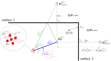
Figure 1: A multipath-based simultaneous localization and mapping (SLAM) scenario at time step $n$, involving two reflective surfaces, a single physical anchor (PA) with position $\bm{p}^{(1)}_{\text{pa}}$, and a single mobile agent with position and orientation, $\bm{p}_{n}$ and $\psi_{n}$, respectively. The mobile agent is depicted with five individual antenna elements at positions $\bm{p}^{(h)}_{n}$, defined by offset $d^{(h)}$ and angle $\psi^{(h)}$. The reflecting surfaces can be represented by “virtual anchor”s (VAs) or master virtual anchors (MVAs), e.g., $\bm{p}^{(1)}_{\text{11,va}}$ or $\bm{p}_{\text{1,mva}}$, respectively. A single-bounce VA represents the location of the mirror image of a PA on the corresponding reflective surface. A MVA represents the location of the mirror image of a common origin on the corresponding reflective surface, thus creating a unique MVA for each reflecting surface. For a second PA or double-bounce propagation path involving surface 1 (not shown),VA positions are different than $\bm{p}^{(1)}_{\text{11,va}}$ while the unique MVA position $\bm{p}_{\text{1,mva}}$ remains the same. Note that $\bm{u}_{1}$ and $\bm{u}_{2}$ are the unit vectors perpendicular to surfaces 1 and 2, while $\bm{e}_{2}$ is an arbitrary vector from the origin to surface 2. Distance and angle for PA and VA at surface 1, i.e., $(d_{00,n}^{(1)},\varphi_{00,n}^{(1)})$ and $(d_{11,n}^{(1)},\varphi_{11,n}^{(1)})$, are also shown.

Emerging sensing technologies and innovative signal processing methods exploiting multipath propagation will lead to new capabilities for autonomous navigation, asset tracking, and situational awareness in future communication networks. Multipath-based SLAM is a promising approach in wireless networks for obtaining position information of transmitters and receivers as well as information on their propagation environments. In multipath-based SLAM, specular reflections of radio frequency (RF) signals at flat surfaces are modeled by “virtual anchor”s (VAs) that are mirror images of base stations, also referred to as physical anchors (PAs) [1]. The number of VAs and their positions are typically unknown. Multipath-based SLAM methods can detect and localize VAs and jointly estimate the time-varying agent position [1, 2, 3, 4, 5]. The availability of VA location information makes it possible to leverage multiple propagation paths of RF signals for agent localization. It can thus significantly improve localization accuracy and robustness [6, 7, 8, 9].

I-A State of the Art

Multipath-based SLAM falls under the umbrella of feature-based SLAM approaches that focus on detecting and mapping distinct features in the environment [10, 11, 12, 13, 14, 15]. In existing multipath-based SLAM methods, the distinct features of interest are the VAs[3, 4, 5, 16, 17] while “measurements” are obtained by extracting parameters from the multipath components of RF signals in preprocessing stage [18, 19, 20, 21]. Measurements can be noisy distances, angles-of-arrival (AoAs), or angles-of-departure (AoDs) [22, 23, 24].

As typical for feature-based SLAM, a complicating factor in multipath-based SLAM is measurement origin uncertainty, i.e., the unknown association of measurements with features [3, 4, 5, 25, 24]. In particular, (i) it is not known which VA was generated by which measurement, (ii) there are missed detections due to low signal-to-noise-ratio (SNR) or occlusion of features, and (iii) there are false positive measurements due to clutter. Thus, an important aspect of multipath-based SLAM is data association between measurements and VAs. Probabilistic data association can increase the robustness and accuracy of multipath-based SLAM but introduces association variables as additional unknown parameters. To avoid the curse of dimensionality related to the high-dimensional parameters space, state-of-the-art methods for multipath-based SLAM perform the SPA on the factor graph representing the underlying statistical model [3, 4, 5]. In addition, since the models for the aforementioned measurements are nonlinear, most methods typically rely on sampling techniques [1, 6, 2, 3, 4, 5]. Recently, multipath-based SLAM was applied to data collected in indoor scenarios by radios with ultra-wide bandwidth [26] or multiple antennas [2, 27, 4].

In existing methods for multipath-based SLAM, each VA represents a single propagation path from an agent to a PA. In particular, even if a reflective surface takes part in multiple propagation paths, each path is represented by a VA, and mapped individually [1, 6, 2, 3, 4, 5, 28]. Existing methods thus neglect inherent geometrical constraints across different paths that interact with the same surface, which limits accuracy and speed. Note that the multipath-based SLAM methods proposed in [29, 16, 17] perform fusion of information provided by multiple cooperating agents. However, these methods are limited to single-bounce paths and do not perform fusion across PAs. In [30, 31, 32, 33], it has been demonstrated that double-bounce paths of RF signals exhibit considerable signal strength and should thus be considered in real-world multipath-based SLAM scenarios. This provides compelling evidence that incorporating information from double-bounce paths can lead to an improved multipath-based SLAM performance.

I-B Contributions and Notations

The problem studied in this paper can be summarized as follows.

Estimate the time-varying position of a mobile agent by making use of the line-of-sight (LOS) and MPCs in RF signals. To leverage the position information of MPCs, the unknown number and positions of reflective surfaces in the environment are estimated during runtime.

We introduce a new statistical model for multipath-based SLAM that considers single-bounce and double-bounce propagation paths and enables data fusion across multiple paths. In existing multipath-based SLAM models, paths represented by VAs are the SLAM features. In the proposed model, however, every reflective surface is directly represented by a SLAM feature referred to as MVA. The MVA representation makes it possible to model inherent geometrical constraints across paths statistically. Following the new model, a factor graph is established, and an extension of the SPAs for multipath-based SLAM in [3, 4, 5] is developed. The resulting SPA can infer reflective surfaces by combining information across multiple propagation paths. Particularly appealing is the ability to fuse paths related to different PA. Within the SPA, ray-tracing (RT) [34, 35, 36] is performed to determine the availability of each single-bounce and double-bounce paths at potential agent positions. The availability check is directly integrated into the statistical model as detection probabilities for propagation paths. The resulting multipath-based SLAM method can provide fast and accurate estimates in scenarios with many reflective surfaces. Note that the proposed method uses distance and angle-of-arrival (AOA) measurements, which have been extracted from the RF signal in a preprocessing stage [18, 19, 20, 21]. The key contributions of this paper are as follows.

• We introduce a statistical model and factor graph for multipath-based SLAM that facilitates data fusion across propagation paths.

• We integrate RT into our statistical model to determine the availability of individual single-bounce and double-bounce propagation path.

• We extend the SPA for multipath-based SLAM [3, 4, 5] based on the introduced factor graph to establish data fusion for multipath-based SLAM.

• We demonstrate significant improvements in estimation performance compared to existing multipath-based SLAM methods based on both simulated and real data.

This paper advances beyond the preliminary account of our method provided in the conference publications [38, 39] by (i) extending the MVAs model to double-bounce propagation paths, (ii) introducing RT to determine the availability of paths and integrating it into the statistical model, (iii) presenting a detailed derivation of the factor graph, and (iv) demonstrating performance advantages compared to reference methods. As reference methods, classical multipath-based SLAM [3, 4], channel-SLAM [2], and multipath-based positioning assuming known VAs positions [40] are considered.

Notation: Random variables are displayed in sans serif, upright fonts; their realizations in serif, italic fonts. Vectors and matrices are denoted by bold lowercase and uppercase letters, respectively. For example, a random variable and its realization are denoted by $\mathsfbr{x}$ and $x$, respectively, and a random vector and its realization by $\bm{\mathsfbr{x}}$ and $\bm{x}$, respectively. Furthermore, $\|\bm{x}\|$ and ${\bm{x}}^{\text{T}}$ denote the Euclidean norm and the transpose of vector $\bm{x}$, respectively, and $\langle\bm{x},\bm{y}\rangle$ denotes the inner-product between the vectors $\bm{x}$ and $\bm{y}$; $\propto$ indicates equality up to a normalization factor; $f(\bm{x})$ denotes the probability density function (PDF) of random vector $\bm{\mathsfbr{x}}$ (this is a short notation for $f_{\bm{\mathsfbr{x}}}(\bm{x})$); $f(\bm{x}|\bm{y})$ denotes the conditional PDF of random vector $\bm{\mathsfbr{x}}$ conditioned on random vector $\bm{\mathsfbr{y}}$ (this is a short notation for $f_{\bm{\mathsfbr{x}}|\bm{\mathsfbr{z}}}(\bm{x}|\bm{z})$). The four-quadrant inverse tangent of position $\bm{p}=[\hskip 0.85358ptp_{1}\hskip 0.85358pt\hskip 0.85358ptp_{2}\hskip 0.85358pt]^{\mathrm{T}}$ is denoted as $\text{atan2}(p_{2},p_{1})$. The cardinality of a set ${\cal{X}}$ is denoted as $|{\cal{X}}|$. $\delta(\cdot)$ denotes the Dirac delta function. Finally, $\delta_{e}$ denotes the indicator function of the event ${e}={0}$ (i.e., $\delta_{e}=1$ if $e={0}$ and ${0}$ otherwise).

II Geometrical Relations

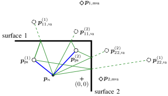
(a)

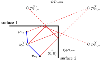
(b)

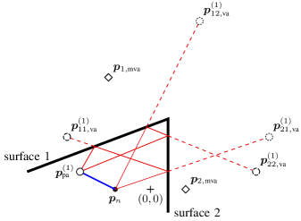
(c)

Figure 2: Three multipath-based SLAMs scenarios with two reflective surfaces illustrate single- and double-bounce paths in three different geometries. The positions of the mobile agents, PAs, VAs, and MVAs are shown. (a) depicts a single time step $n$ of a scenario with perpendicular reflective surfaces, two PAs at positions $\bm{p}_{\text{pa}}^{(1)}$ and $\bm{p}_{\text{pa}}^{(2)}$, and the agent at position $\bm{p}_{n}$; only single-bounce paths are illustrated. (b) shows perpendicular reflective surfaces, one PA at position $\bm{p}_{\text{pa}}^{(1)}$, and agent positions $\bm{p}_{n_{1}}$ and $\bm{p}_{n_{2}}$ at two different time steps $n_{1}$ and $n_{2}$. Only double-bounce paths are shown. (c) depicts a single time step $n$ of a scenario with reflective surfaces at an acute angle, one PA at position $\bm{p}_{\text{pa}}^{(1)}$ and the agent at position $\bm{p}_{n}$. Again, only double-bounce paths are illustrated. Note that in (b), due to perpendicular reflective surfaces, both double-bounce paths have equal lengths, and there is a single double-bounce VA. In (b), however, due to reflective surfaces at an acute angle, the two double-bounce paths have different lengths, and there are two different double-bounce VAs.

We consider a mobile agent equipped with an $H$-element antenna array and $J$ PAs equipped with a single antenna at known positions $\bm{p}_{\mathrm{pa}}^{(j)}=\big{[}{p}_{1,\mathrm{pa}}^{(j)}\hskip 0.85358pt\hskip 0.85358pt\hskip 0.85358pt{p}_{2,\mathrm{pa}}^{(j)}\big{]}^{\mathrm{T}}\!\in\mathbb{R}^{2}$, $j\in\{1,\ldots,J\}$, where $J$ is assumed to be known. The agent is in an environment with $S$ reflective surfaces indexed by $s\in{\cal{S}}\triangleq\{1,\ldots,S\}$. At every discrete time step $n$, the array element locations are denoted by $\bm{p}_{n}^{(h)}$, $h\in\{1,\dots,H\}$. The agent position $\bm{p}_{n}$ refers to the center of gravity of the array. We also define $d^{(h)}=\|\bm{p}_{n}^{(h)}-\bm{p}_{n}\|$ and $\psi^{(h)}=\text{atan2}\big{(}{p}_{2,n}^{(h)}-{p}_{2,n},{p}_{1,n}^{(h)}-{p}_{1,n}\big{)}-\psi_{n}$, the distance from the reference location $\bm{p}_{n}$ and the orientation, respectively, of the $h$-th element as shown in Fig. 1. At each discrete time slot $n$, the position $\bm{p}_{n}\!\in\mathbb{R}^{2}$ and the array orientation $\psi_{n}$ of the agent are unknown. Each PA transmits a RF signal, and the agent acts as a receiver. The RF signal arrives at the receiver via the LOS path as well as via MPCs originating from the reflection of surrounding objects. We assume time synchronization between all PAs and the agent. However, our algorithm can be extended to an unsynchronized system according to [2, 6, 41].

We restrict the representation to MPCs related to single-bounce and double-bounce paths. In particular, associated with PA $j$ there are $|{\cal{D}}_{\text{S}}|=S$ single-bounce VAs [34, 3] at unknown positions $\bm{p}_{ss,\mathrm{va}}^{(j)}\!\in\mathbb{R}^{2}$ with index-pair $(s,s)\in{\cal{D}}_{\text{S}}\triangleq\{(s,s)\in{\cal{S}}\times{\cal{S}}\}$ and $|{\cal{D}}_{\text{D}}|=S(S-1)$ double-bounce VAs at unknown positions $\bm{p}_{ss^{\prime},\mathrm{va}}^{(j)}\!\in\mathbb{R}^{2}$ with index-pair $(s,s^{\prime})\in{\cal{D}}_{\text{D}}\triangleq\{(s,s^{\prime})\in{\cal{S}}\times{\cal{S}}|\hskip 0.85358pts\neq s^{\prime}\}$. Therefore, the maximum number of VAs for PA $j$ is given by $|\mathcal{D}|=S+S(S-1)$ with ${\cal{D}}\triangleq\{(s,s^{\prime})\in{\cal{S}}\times{\cal{S}}\}={\cal{D}}_{\text{D}}\cup{\cal{D}}_{\text{S}}$. Note that subscript indices denoted as $(\cdot)_{ss^{\prime}}$ indicate variables related to a pairs $(s,s^{\prime})$ of reflecting objects. By applying the image-source model [34, 42], a VA associated with a single-bounce path is the mirror image of $\bm{p}_{\mathrm{pa}}^{(j)}$ at reflective surface $s\in\mathcal{S}$ given by

$$\bm{p}^{(j)}_{ss,\mathrm{va}} =\bm{p}^{(j)}_{\mathrm{pa}}+2\big{(}\bm{u}_{s}^{\text{T}}\bm{e}_{s}-\bm{u}_{s}^{\text{T}}\bm{p}^{(j)}_{\mathrm{pa}}\big{)}\bm{u}_{s}$$ (1)

where $(s,s)\in{\cal{D}}_{\text{S}}$, $\bm{u}_{s}$ is the normal vector of reflective surface $s$, and $\bm{e}_{s}$ is an arbitrary point on the considered surface. The second term in (1) represents the normal vector w.r.t. to reflective surface $s$ in direction $\bm{u}_{s}$ with the length of two times the distance between PA $j$ at position $\bm{p}^{(j)}_{\mathrm{pa}}$ and the normal-point at the reflective surface $s$, i.e., $2\big{(}\bm{u}_{s}^{\text{T}}\bm{e}_{s}-\bm{u}_{s}^{\text{T}}\bm{p}^{(j)}_{\mathrm{pa}}\big{)}$. By again applying the image-source model [34, 42] for VA at position $\bm{p}^{(j)}_{s^{\prime}s^{\prime},\mathrm{va}}$ another VA that is obtained as the mirror image of $\bm{p}^{(j)}_{s^{\prime}s^{\prime},\mathrm{va}}$ at surface $s$, i.e.,

$$\bm{p}^{(j)}_{ss^{\prime},\mathrm{va}} =\bm{p}^{(j)}_{s^{\prime}s^{\prime},\mathrm{va}}+2\big{(}\bm{u}_{s}^{\text{T}}\bm{e}_{s}-\bm{u}_{s}^{\text{T}}\bm{p}^{(j)}_{s^{\prime}s^{\prime},\mathrm{va}}\big{)}\bm{u}_{s}$$ (2)

where $(s,s^{\prime})\in{\cal{D}}_{\text{D}}$. This VA represents a double-bounce propagation path. For conveniently addressing PA-related variables and factors, we also define $\bm{p}^{(j)}_{00,\mathrm{va}}\triangleq\bm{p}^{(j)}_{\mathrm{pa}}$ and ${\tilde{\mathcal{D}}}=(0,0)\cup{\mathcal{D}}$. The distances and AOAs related to the propagation paths at the agent position $\bm{p}_{n}$ represented by $\bm{p}_{ss^{\prime},\mathrm{va}}^{(j)}$ with $(s,s^{\prime})\in{\tilde{\mathcal{D}}}$ are modeled by $d_{ss^{\prime},n}^{(j)}=\big{\|}\bm{p}_{n}-\bm{p}^{(j)}_{ss^{\prime},\mathrm{va}}\big{\|}$ and $\varphi_{ss^{\prime},n}^{(j)}=\text{atan2}\big{(}{p}_{2,n}-{p}^{(j)}_{1,ss^{\prime},\text{va}},{p}_{1,n}-{p}^{(j)}_{1,ss^{\prime},\text{va}}\big{)}-\psi_{n}$. Note that the distance $d_{00,n}^{(j)}$ and the AOAs $\varphi_{00,n}^{(j)}$ are the parameters related to the LOS path between agent at position $\bm{p}_{n}$ and PA $j$ at position $\bm{p}^{(j)}_{\mathrm{pa}}$. An example is shown in Fig. 1.

The availability of VAs at certain agent position $\bm{p}_{n}$ is limited due to blockage of associated propagation paths or geometric constraints between reflective surfaces [34, 35]. Especially, double-bounce paths and their corresponding VA positions have limited availability depending on the agent position $\bm{p}_{n}$ (see Fig. 2b and Fig. 2c). Hence, the number of available VAs for PA $j$ is smaller than $|\mathcal{D}|=S+S(S-1)$. As discussed in Section III-D, the proposed statistical model and method performs an availability check for each VA using RT [34, 35, 36]. In this way, for each agent position $\bm{p}_{n}$, it can be determine which of the potential paths in $\mathcal{D}$ is available.

TABLE I: Notations and definitions of important quantities.

Notation	Definition	Notation	Definition
$\bm{p}_{\mathrm{pa}}^{(j)}$	2D position of physical anchor $j$	$\bm{p}_{n}$	2D position of mobile agent at time $n$
$\psi_{n}$	Orientation of mobile agent at time $n$	$\bm{v}_{n}$	2D velocity of mobile agent at time $n$
$S$	Total number of reflecting surfaces (MVAs)	$\mathsfbr{M}^{(j)}_{n}$	Number of measurements with PA $j$ at time $n$
$\bm{p}_{ss,\mathrm{va}}^{(j)}$	Single-bounce virtual anchor position	$\bm{p}_{ss^{\prime},\mathrm{va}}^{(j)}$	Double-bounce virtual anchor position
$\bm{p}_{s,\mathrm{mva}}$	Position of MVA corresponding to PA $s$	$S_{n}$	Number of potential s at time $n$
${\mathsfbr{z}_{\text{d}}}_{m,n}^{(j)}$	Distance measurement $m$ with PA $j$ at time $n$	${\mathsfbr{z}_{\varphi}}_{m,n}^{(j)}$	angle-of-arrival measurement $m$ with PA $j$ at time $n$
${\snu_{\mathrm{\tau}}}_{m,n}^{(j)}$	Distance measurement noise	${\nu_{\mathrm{\varphi}}}_{m,n}^{(j)}$	angle-of-arrival measurement noise
$\mathsfbr{r}_{s,n}$	Binary existence variable related to PMVA $s$ at time $n$	$p_{\mathrm{d},ss^{\prime},n}^{(j)}$	detection probability of available path
$\mu_{\mathrm{fp}}$	False alarm Poisson point process mean	$f_{\mathrm{fp}}(\bm{\mathsfbr{z}}_{m,n}^{(j)})$	False positive point process PDF
$p_{\mathrm{s}}$	Probability of survival of legacy PMVA	$p_{\mathrm{cf}}$	Confirmation threshold for PMVAs
$p_{\text{pr}}$	Pruning threshold to remove PMVAs	$\Delta T$	Simulation sampling period
$\bm{\omega}_{n}$	Process noise of the agents’ motion model

II-A MVA-Based Model of the Environment

A reflective surface is involved in multiple propagation paths and thus defines multiple VAs. To enable the consistent combination, i.e., “fusion” of map information provided by measurements of different PAs, we represent reflective surfaces by $S$ unique MVAs at positions $\bm{p}_{s,\mathrm{mva}}\!\in\mathbb{R}^{2}$, $s\in{\cal{S}}$. The unique MVA position $\bm{p}_{s,\mathrm{mva}}\!\in\mathbb{R}^{2}$ is defined as the mirror image of $[0\hskip 1.70717pt0]^{\text{T}}$ on the reflective surface $S$. By using some algebra, the transformation from MVA at $\bm{p}_{s,\mathrm{mva}}$ to a VA at $\bm{p}^{(j)}_{ss,\mathrm{va}}$, i.e., $\bm{p}^{(j)}_{ss,\mathrm{va}}=h_{\text{va}}\big{(}\bm{p}_{s,\mathrm{mva}},\bm{p}^{(j)}_{\mathrm{pa}}\big{)}$ can be obtained as

$$\bm{p}^{(j)}_{ss,\mathrm{va}}=-\bigg{(}\frac{2\big{\langle}\bm{p}_{s,\mathrm{mva}},\bm{p}^{(j)}_{\mathrm{pa}}\big{\rangle}}{\big{\|}\bm{p}_{s,\mathrm{mva}}\big{\|}^{2}}-1\bigg{)}\hskip 0.85358pt\bm{p}_{s,\mathrm{mva}}+\hskip 0.85358pt\bm{p}^{(j)}_{\mathrm{pa}}\hskip 0.85358pt.$$ (3)

The transformation from MVAs at $\bm{p}_{s,\mathrm{mva}}$ and $\bm{p}_{s^{\prime},\mathrm{mva}}$ to a double-bounce VA at $\bm{p}^{(j)}_{ss^{\prime},\mathrm{va}}$ can be obtained by applying (3) twice, i.e, $\bm{p}^{(j)}_{ss^{\prime},\text{va}}=h_{\text{va}}\big{(}\bm{p}_{s,\mathrm{mva}},h_{\text{va}}\big{(}\bm{p}_{s^{\prime},\mathrm{mva}},\bm{p}^{(j)}_{\mathrm{pa}}\big{)}\big{)}$. The inverse transformation from a VA to a MVA is given by

$$\bm{p}_{s,\mathrm{mva}} =h_{\text{mva}}\big{(}\bm{p}^{(j)}_{ss,\mathrm{va}},\bm{p}^{(j)}_{\mathrm{pa}}\big{)}$$

$$=\frac{\big{\|}\bm{p}^{(j)}_{\mathrm{pa}}\big{\|}^{2}-\big{\|}\bm{p}^{(j)}_{ss,\mathrm{va}}\big{\|}^{2}}{\big{\|}(\bm{p}^{(j)}_{\mathrm{pa}}-\bm{p}^{(j)}_{ss,\mathrm{va}})\big{\|}^{2}}\big{(}\bm{p}^{(j)}_{\mathrm{pa}}-\bm{p}^{(j)}_{ss,\mathrm{va}}\big{)}\hskip 0.85358pt.$$ (4)

Note that the inverse transformation in (4) will be used to determine a proposal distribution for MVA states as discussed in Section V. Details of the derivation of (3) and (4) are provided in the supplementary material[37, Section LABEL:M-sec:app_mva_model]. For example, Fig. 2 shows three scenarios with two reflecting surfaces described by two MVAs at positions $\bm{p}_{1,\mathrm{mva}}$ and $\bm{p}_{2,\mathrm{mva}}$. Fig. 2a shows a scenario with two PAs $j\in\{1,2\}$, the corresponding VAs, and an agent at position $\bm{p}_{n}$. Each PA generates one VA associated with a single-bounce propagation path. Fig. 2b shows a scenario with one PA, the corresponding VAs associated with single-bounce and double-bounce propagation paths, and two agents positions at differnet time steps, i.e., $\bm{p}_{n_{1}}$ and $\bm{p}_{n_{2}}$. Note in case surfaces are perpendicular, a different order of bounces from surfaces, i.e., surface “$s$ – surface $s^{\prime}$” or “surface $s^{\prime}$ – surface $s$”, does not lead to a different VA position. Depending on the agent position $\bm{p}_{n}$, only one double-bounce propagation path (related to one of the two orders) is available (see also Section III-D). Fig. 2b shows a scenario with non-perpendicular surfaces. In this case, different “bounce orders” lead to different VA-positions. In particular, if there is an acute angle between a pair of reflecting surfaces, there exist regions of agent positions $\bm{p}_{n}$ for which two double-bounce propagation paths are available at the same time (cf. Section III-D). These regions depend on the PA position as well as the angle between the two surfaces. Note that when the angle between a pair is obtuse, only one of the two double-bounce propagation paths is available for all positions $\bm{p}_{n}$ (an example is given in [37, Section LABEL:M-sec:app_results]).

III System Model

At each time $n$, the state of the agent is given by $\bm{\mathsfbr{x}}_{n}=[\bm{\mathsfbr{p}}_{n}^{\text{T}}\hskip 2.84526pt\bm{\mathsfbr{v}}_{n}^{\text{T}}]$, where $\bm{\mathsfbr{v}}_{n}$ is the agent velocity vector. We assume that the array is rigidly coupled with the movement direction, i.e., array orientation is determined by the direction of the agent velocity vector. As in [43, 44, 3], we account for the unknown number of MVAs by introducing potential (PMVA) $s\in{\cal{S}}_{n}\triangleq\{1,\dots,\mathsfbr{S}_{n}\}$. The number $S_{n}$ of PMVAs is the maximum possible number of actual MVAs, i.e., all MVAs that produced a measurement so far [44, 3] (where $S_{n}$ increases with time). PMVA states are denoted as $\bm{\mathsfbr{y}}_{s,n}=\big{[}\bm{\mathsfbr{p}}^{\text{T}}_{s,\mathrm{mva}}\;\mathsfbr{r}_{s,n}\big{]}^{\text{T}}$. The existence/nonexistence of PMVA $s$ is modeled by the existence variable $\mathsfbr{r}_{s,n}\in\{0,1\}$ in the sense that PMVA $s$ exists if $r_{s,n}=1$. Formally, its states is considered even if PMVA $s$ is nonexistent, i.e., if $r_{s,n}=0$. The states $\bm{\mathsfbr{p}}^{\text{T}}_{s,\mathrm{mva}}$ of nonexistent PMVAs are obviously irrelevant. Therefore, all PDFs defined for PMVA states, $f(\bm{\mathsfbr{y}}_{s,n})=f(\bm{\mathsfbr{p}}_{s,\mathrm{mva}},\mathsfbr{r}_{s,n})$, are of the form $f(\bm{\mathsfbr{p}}_{s,\mathrm{mva}},0)=f_{s,n}f_{\text{d}}(\bm{\mathsfbr{p}}_{s,\mathrm{mva}})$, where $f_{\text{d}}(\bm{\mathsfbr{p}}_{s,\mathrm{mva}})$ is an arbitrary “dummy PDF” and $f_{s,n}\!\in[0,1]$ is a constant and can be interpreted as the probability of non-existence [44, 3]. A summary of all variables related to agent and PMVA states as well as other variables of the proposed statistical model can be found in Table I.

III-A Measurements and New PMVAs

The distance and AOA measurements related to the path “agent at position $\bm{\mathsfbr{p}}_{n}$ – VA at position $\bm{\mathsfbr{p}}^{(j)}_{ss^{\prime},\text{va}}$” with $(s,s^{\prime})\in\tilde{{\cal{D}}}_{n}$ are given by

$${\mathsfbr{z}_{\text{d}}}_{m,n}^{(j)} =\big{\|}\bm{\mathsfbr{p}}_{n}-\bm{p}^{(j)}_{ss^{\prime},\mathrm{va}}\big{\|}+{\snu_{\mathrm{d}}}_{m,n}^{(j)}$$ (5)

$${\mathsfbr{z}_{\varphi}}_{m,n}^{(j)} =\text{atan2}\big{(}{p}_{2,n}-{p}^{(j)}_{2,ss^{\prime},\mathrm{va}},{p}_{1,n}-{p}^{(j)}_{1,ss^{\prime},\mathrm{va}}\big{)}$$

$$\hskip 14.22636pt{-\text{atan2}\big{(}{v}_{2,n},{v}_{1,n}\big{)}}+{\snu_{\mathrm{\varphi}}}_{m,n}^{(j)}$$ (6)

where ${\snu_{\mathrm{d}}}_{m,n}^{(j)}$ and ${\snu_{\mathrm{\varphi}}}_{m,n}^{(j)}\vspace*{-0.8mm}$ are, respectively, zero-mean Gaussian measurement noise with standard deviations ${\sigma_{\mathrm{d}}}^{(j)}_{m,n}\vspace*{0.2mm}$ and ${\sigma_{\mathrm{\varphi}}}^{(j)}_{m,n}$. The measurements are combined in the vector $\bm{\mathsfbr{z}}_{m,n}^{(j)}=[{\mathsfbr{z}_{\text{d}}}_{m,n}^{(j)}\hskip 2.84526pt{\mathsfbr{z}_{\varphi}}_{m,n}^{(j)}]^{\text{T}}$ with $m\in{\cal{M}}_{n}^{(j)}\triangleq\{1,$ $\dots,\mathsfbr{M}^{(j)}_{n}\}$ for PA $j$. (These measurements represent the MPC parameters. For details see [4, 2, 24].) Note that before measurements are acquired, the number of measurements $\mathsfbr{M}^{(j)}_{n}$ is random.

Likelihood function for LOS paths: Using (5), (6), and $\bm{p}^{(j)}_{00,\text{va}}=\bm{p}^{(j)}_{\mathrm{pa}}$, we can directly obtain the likelihood function for the LOS path as $f\big{(}\bm{z}_{m,n}^{(j)}\big{|}\bm{p}_{n}\big{)}\vspace{.8mm}$.

Likelihood function for single-bounce paths: Using (5), (6), and the transformation in (3), i.e., $\bm{\mathsfbr{p}}^{(j)}_{ss,\text{va}}={h_{\text{va}}}\big{(}\bm{\mathsfbr{p}}_{s,\mathrm{mva}},\bm{p}^{(j)}_{\mathrm{pa}}\big{)}$, the likelihood function related to the single-bounce propagation path “agent – surface $s$” with $s\in{\cal{S}}$ – PA $j$ with MVA index-pair $(s,s)\in\mathcal{D}_{\text{S},n}$ reads $f(\bm{z}_{m,n}^{(j)}|\bm{p}_{n},\bm{p}_{s,\mathrm{mva}})\vspace{.8mm}$.

Likelihood function for double-bounce paths: Using (5), and (6), and the transformation in (3) twice, i.e., $\bm{\mathsfbr{p}}^{(j)}_{ss^{\prime},\text{va}}={h_{\text{va}}}\big{(}\bm{\mathsfbr{p}}_{s,\mathrm{mva}},{h_{\text{va}}}\big{(}\bm{\mathsfbr{p}}_{s^{\prime},\mathrm{mva}},\bm{p}^{(j)}_{\mathrm{pa}}\big{)}\big{)}$, the likelihood function related to the double-bounce path “agent – surface $s$ – surface $s^{\prime}$ – PA $j$” with MVA index-pair $(s,s^{\prime})\in\mathcal{D}_{\text{D},n}$ can be expressed by $f(\bm{z}_{m,n}^{(j)}|,\bm{p}_{n},\bm{p}_{s,\mathrm{mva}},\bm{p}_{s^{\prime},\mathrm{mva}})\vspace{.8mm}$.

With the MVA-based measurement model, at time $n$, the measurements collected by all PAs $j\in\{1,\dots,J\}$ can provide information on the same MVA and agent positions $\bm{\mathsfbr{p}}_{s,\mathrm{mva}},s\in{\cal{S}}$ and $\bm{\mathsfbr{p}}_{n}$, respectively. It is assumed that each VA (related to a specific PA, MVA or MVA-MVA pair) generates at most one measurement and that a measurement originates from at most one VA. PA $j$ at position $\bm{p}^{(j)}_{00,\text{va}}=\bm{p}^{(j)}_{\mathrm{pa}}$ with $(0,0)\in\tilde{{\cal{D}}}_{n}$ generates a measurements $\bm{\mathsfbr{z}}_{m,n}^{(j)}$ with detection probability $p^{(j)}_{\mathrm{d}}\big{(}\bm{\mathsfbr{p}}_{n}\big{)}$. If MVA $s$ exists ($r_{s,n}=1$), the corresponding single-bounce path $(s,s)\in{\cal{D}}_{\text{S},n}$ generates a MVA-originated measurements $\bm{\mathsfbr{z}}_{m,n}^{(j)}$ with detection probability $p^{(j)}_{\mathrm{d}}\big{(}\bm{\mathsfbr{p}}_{n},\bm{\mathsfbr{p}}_{s,\text{mva}}\big{)}$. The same holds for the double-bounce path $(s,s^{\prime})\in{\cal{D}}_{\text{D},n}$ with detection probability $p^{(j)}_{\mathrm{d}}\big{(}\bm{\mathsfbr{p}}_{n},\bm{\mathsfbr{p}}_{s,\text{mva}},\bm{\mathsfbr{p}}_{s^{\prime},\text{mva}}\big{)}$. Note that the detection probability is determined by the SNR of the measurement [4] as well as the availability check performed by RT. In particular, if a path is unavailable, its detection probability is set to zero. A measurement $\bm{\mathsfbr{z}}_{m,n}^{(j)}$ may also not originate from any MVA. This type of measurement is referred to as a false positive and is modeled as a Poisson point process with mean $\mu_{\mathrm{fp}}$ and PDF $f_{\mathrm{fp}}(\bm{\mathsfbr{z}}_{m,n}^{(j)})$.

Newly detected MVAs, i.e., MVAs that generated a measurement for the first time, are modeled by a Poisson point process with mean $\mu_{\mathrm{n}}$ and PDF $f_{\mathrm{n}}(\bm{p}_{m,\mathrm{mva}}|\bm{p}_{n})$. Newly detected MVAs are represented by new PMVA states $\overline{\bm{\mathsfbr{y}}}^{(j)}_{n,m}$, $m\in\{1,\dots,\mathsfbr{M}^{(j)}_{n}\}$ in our statistical model [44, 3]. Each new PMVA state corresponds to a measurement $\bm{\mathsfbr{z}}_{m,n}^{(j)}$; $\overline{r}_{m,n}\!=\!1$ implies that measurement $\bm{\mathsfbr{z}}_{m,n}^{(j)}$ was generated by a newly detected MVA. All new PMVA states are introduced, assuming the corresponding measurements originate from a single-bounce path. This assumption leads to a simpler statistical model and reduced computational complexity as further discussed in Section V-D. This assumption is well motivated by the fact that, due to the lower SNR of double-bounce paths, new surfaces are typically detected first via a single-bounce measurement. However, the assumption also implies that any reflecting surface can only be mapped if it originates at least one single-bounce measurement.

We denote by $\overline{\bm{\mathsfbr{y}}}^{(j)}_{n}\triangleq\big{[}\hskip 0.85358pt\overline{\bm{\mathsfbr{y}}}^{(j)\hskip 0.85358pt\text{T}}_{1,n}\cdots\hskip 0.85358pt\overline{\bm{\mathsfbr{y}}}^{(j)\hskip 0.85358pt\text{T}}_{\mathsfbr{M}^{(j)}_{n},n}\hskip 0.85358pt\big{]}^{\text{T}}$, the joint vector of all new PMVA states. Introducing new PMVA for each measurement leads to a number of PMVA states that grows with time $n$. Thus, to keep the proposed SLAM algorithm feasible, a sub-optimum pruning step is performed, removing PMVAs with a low probability of existence (see Section IV-B).

III-B Legacy PMVAs and State Transition

At time $n$, measurements are incorporated sequentially across PAs $j\in\{1,\dots,J\}$. Previously detected MVAs, i.e., MVAs that have been detected either at a previous time $n^{\prime}\!<n$ or at the current time $n$ but at a previous PA $j^{\prime}\!<j$, are represented by legacy PMVA states $\underline{\bm{\mathsfbr{y}}}_{s,n}^{(j)}$. New PMVAs become legacy PMVAs when the next measurements—either of the next PA or at the next time instance—are taken into account. In particular, the MVA represented by the new MVA state $\overline{\bm{\mathsfbr{y}}}^{(j^{\prime})}_{m^{\prime},n^{\prime}}$ introduced due to measurement $m^{\prime}$ of PA $j^{\prime}$ at time $n^{\prime}\leqslant n$ is represented by the legacy PMVA state $\underline{\bm{\mathsfbr{y}}}^{(j)}_{s,n}$ at time $n$, with $s=\mathsfbr{S}_{n^{\prime}-1}+\sum^{j^{\prime}-1}_{j^{\prime\prime}=1}\mathsfbr{M}^{(j^{\prime\prime})}_{n}+m^{\prime}\vspace{.5mm}$. The number of legacy PMVA at time $n$, when the measurements of the next PA $j$ are incorporated, is updated according to $\mathsfbr{S}^{(j)}_{n}=\mathsfbr{S}^{(j-1)}_{n}+\mathsfbr{M}^{(j-1)}_{n}$, where $\mathsfbr{S}^{(1)}_{n}=\mathsfbr{S}_{n-1}$. Here, $\mathsfbr{S}^{(j)}_{n}$ is equal to the number of all measurements collected up to time $n$ and PA $j-1$. The vector of all legacy PMVA states at time $n$ and up to PA $j$ can now be written as $\underline{\bm{\mathsfbr{y}}}^{(j)}_{n}=\big{[}\underline{\bm{\mathsfbr{y}}}^{(j-1)\text{T}}_{n}\hskip 0.85358pt\hskip 0.85358pt\hskip 0.85358pt\overline{\bm{\mathsfbr{y}}}^{(j-1)\text{T}}_{n}\big{]}^{\text{T}}$.

Let us denote by $\underline{\bm{\mathsfbr{y}}}^{(1)}_{n}\triangleq\big{[}\underline{\bm{\mathsfbr{y}}}^{\text{T}}_{1,n}\cdots\hskip 0.85358pt\underline{\bm{\mathsfbr{y}}}^{T}_{S_{n-1},n}\big{]}^{\text{T}}$, the vector of all legacy PMVA states before any measurements at time $n$ have been incorporated. After the measurements of all PAs $j\in\{1,\dots,J\}$ have been incorporated at time $n$, the total number of PMVA states is

$$\mathsfbr{S}_{n}=\mathsfbr{S}_{n-1}+\sum_{j=1}^{J}\mathsfbr{M}^{(j)}_{n}=\mathsfbr{S}^{(J)}_{n}+\mathsfbr{M}^{(J)}_{n}$$ (7)

and the vector of all PMVA states at time $n$ is given by $\bm{\mathsfbr{y}}_{n}\!=\big{[}\underline{\bm{\mathsfbr{y}}}^{(J)\text{T}}_{n}\hskip 0.85358pt\hskip 0.85358pt\overline{\bm{\mathsfbr{y}}}^{(J)\text{T}}_{n}\big{]}^{\text{T}}$. We also define the number of VAs for each PA given as $|\mathcal{D}^{(j)}_{n}|=\mathsfbr{S}^{(j)}_{n}+\mathsfbr{S}^{(j)}_{n}(\mathsfbr{S}^{(j)}_{n}-1)$ with $\mathcal{D}^{(j)}_{n}\in\{(s,s^{\prime})\in{\cal{S}}_{n}\times{\cal{S}}_{n}\}={\cal{D}}_{\text{S},n}^{(j)}\cup{\cal{D}}_{\text{D},n}^{(j)}$ and $\tilde{\mathcal{D}}^{(j)}_{n}=(0,0)\cup\mathcal{D}^{(j)}_{n}$.

Legacy PMVAs states $\underline{\bm{\mathsfbr{y}}}_{s,n}$ and the agent state $\bm{\mathsfbr{x}}_{n}$ are assumed to evolve independently across time according to state-transition PDFs $f\big{(}\underline{\bm{y}}_{s,n}\big{|}\bm{y}_{s,n-1}\big{)}$ and $f(\bm{x}_{n}|\bm{x}_{n-1})$, respectively. If PMVA $k$ exists at time $n-\!1$, i.e., $r_{s,n-1}\!=\!1$, it either disappears, i.e., $\overline{r}_{s,n}\!=0$, or survives, i.e., $\overline{r}_{s,n}\!=\!1$; in the latter case, it becomes a legacy PMVA at time $n$. The probability of survival is denoted by $p_{\mathrm{s}}$. Suppose the PMVA survives. In that case, its position remains unchanged, i.e., the state-transition pdf of the MVA positions $\underline{\bm{\mathsfbr{p}}}_{s,\mathrm{mva}}$ is given by $f\big{(}\underline{\bm{p}}_{s,\mathrm{mva}}\hskip 0.85358pt\big{|}\hskip 0.85358pt\bm{p}_{s,\mathrm{mva}}\big{)}=\delta\big{(}\underline{\bm{p}}_{s,\mathrm{mva}}-\hskip 0.85358pt\bm{p}_{s,\mathrm{mva}}\big{)}$. Therefore, $f\big{(}\underline{\bm{p}}_{s,\mathrm{mva}},\underline{r}_{s,n}\hskip 0.85358pt\big{|}\hskip 0.85358pt\bm{p}_{s,\mathrm{mva}},r_{s,n-1}\big{)}$ for $r_{s,n-1}=1$ is obtained as

$$f\big{(}\underline{\bm{p}}_{s,\mathrm{mva}},\underline{r}_{s,n}\hskip 0.85358pt\big{|}\hskip 0.85358pt\bm{p}_{s,\mathrm{mva}},r_{s,n-1}=1\big{)}$$

$$\hskip 48.36967pt=\begin{cases}(1\!-p_{\mathrm{s}})\hskip 0.85358ptf_{\text{d}}\big{(}\underline{\bm{p}}_{s,\mathrm{mva}}\big{)},&\!\!\!\underline{r}_{s,n}\!=0\\[0.0pt] p_{\mathrm{s}}\hskip 0.85358pt\hskip 0.85358pt\delta\big{(}\underline{\bm{p}}_{s,\mathrm{mva}}-\hskip 0.85358pt\bm{p}_{s,\mathrm{mva}}\big{)},&\!\!\!\underline{r}_{s,n}\!=\!1.\end{cases}$$ (8)

If MVA $s$ does not exist at time $n-\!1$, i.e., $r_{s,n-1}\!=\!0$, it cannot exist as a legacy PMVA at time $n$ either, thus we get

$$f\big{(}\underline{\bm{p}}_{s,\mathrm{mva}},\underline{r}_{s,n}\big{|}\bm{p}_{s,\mathrm{mva}},r_{s,n-1}=0\big{)}$$

$$\hskip 76.82243pt=\begin{cases}f_{\text{d}}\big{(}\underline{\bm{p}}_{s,\mathrm{mva}}\big{)},&\!\!\!\underline{r}_{s,n}\!=0\\[0.0pt] 0,&\!\!\!\underline{r}_{s,n}\!=\!1.\end{cases}$$ (9)

For $j\geqslant 2$, we also define $f^{(j)}\big{(}\underline{\bm{y}}^{(j)}_{s,n}\big{|}\underline{\bm{y}}^{(j-1)}_{s,n}\big{)}$ as

$$f^{(j)}\big{(}\underline{\bm{p}}^{(j)}_{s,\mathrm{mva}},\underline{r}^{(j)}_{s,n}\hskip 0.85358pt\big{|}{\hskip 0.85358pt\underline{\bm{p}}^{(j-1)}_{s,\mathrm{mva}},\underline{r}^{(j-1)}_{s,n}=1}\big{)}$$

$$\hskip 48.36967pt=\begin{cases}f_{\text{d}}\big{(}\underline{\bm{p}}^{(j-1)}_{s,\mathrm{mva}}\big{)},&\!\!\!\underline{r}^{(j)}_{s,n}\!=0\\[0.0pt] \delta\big{(}\underline{\bm{p}}^{(j)}_{s,\mathrm{mva}}-\hskip 0.85358pt\underline{\bm{p}}^{(j-1)}_{s,\mathrm{mva}}\big{)},&\!\!\!\underline{r}^{(j)}_{s,n}\!=\!1\end{cases}$$ (10)

and

$$f^{(j)}\big{(}\underline{\bm{p}}^{(j)}_{s,\mathrm{mva}},\underline{r}^{(j)}_{s,n}\big{|}{\underline{\bm{p}}^{(j-1)}_{s,\mathrm{mva}},\underline{r}^{(j-1)}_{s,n}=0}\big{)}$$

$$\hskip 76.82243pt=\begin{cases}f_{\text{d}}\big{(}\underline{\bm{p}}^{(j)}_{s,\mathrm{mva}}\big{)},&\!\!\!\underline{r}^{(j)}_{s,n}\!=0\\[0.0pt] 0,&\!\!\!\underline{r}^{(j)}_{s,n}\!=\!1.\end{cases}$$ (11)

where we introduced $\underline{\bm{y}}^{(j-1)}_{s,n}\triangleq\underline{\bm{y}}_{s,n}$, $\bm{p}^{(j-1)}_{s,\mathrm{mva}}\triangleq\bm{p}_{s,\mathrm{mva}}$, and $\underline{r}^{(j-1)}_{s,n}\triangleq\underline{r}_{s,n}$. It it assumed that at time $n=0$ the initial prior PDF $f\big{(}\bm{y}_{s,0}\big{)}$, $s=\big{\{}1,\dots,S_{0}\big{\}}$ and $f(\bm{x}_{0})$ are known. All (legacy and new) PMVA states and all agent states up to time $n$ are denoted as $\bm{\mathsfbr{y}}_{0:n}\triangleq\big{[}\bm{\mathsfbr{y}}^{\text{T}}_{0}\cdots\hskip 0.85358pt\bm{\mathsfbr{y}}^{\text{T}}_{n}\big{]}^{\text{T}}\!$ and $\bm{\mathsfbr{x}}_{0:n}\triangleq\big{[}\bm{\mathsfbr{x}}^{\text{T}}_{0}\cdots\hskip 0.85358pt\bm{\mathsfbr{x}}^{\text{T}}_{n}\big{]}^{\text{T}}\!$, respectively.

III-C Data Association Uncertainty

Mapping of reflective surfaces modeled by MVA is complicated by the data association uncertainty: at time $n$ it is unknown which measurement $\bm{\mathsfbr{z}}_{m,n}^{(j)}$ extracted at PA $j$ originated from PA $j$ itself $(0,0)$, from which MVA $(s,s)\in\mathcal{D}^{(j)}_{\text{S},n}$, or from which MVA-MVA pair $(s,s^{\prime})\in\mathcal{D}^{(j)}_{\text{D},n}$ associated with single-bounce and double-bounce path. Any PMVA-to-measurement association (which considers associations to single PMVAs and PMVA-PMVA pairs as well as to PA $j$ itself) is described by PMVA-oriented association variables

$$\mathsfbr{\underline{a}}^{(j)}_{ss^{\prime},n}\hskip 0.85358pt\triangleq\begin{cases}m\in{\cal{M}}_{n}^{(j)}\hskip 0.85358pt,&\begin{minipage}[t]{128.0374pt}if legacy \acs{pmva} $ss^{\prime}$ generates measurement $m$\\ \end{minipage}\\[11.38109pt] 0\hskip 0.85358pt,&\begin{minipage}[t]{128.0374pt}if legacy \acs{pmva} $ss^{\prime}$ does not generate any measurement\\ \end{minipage}\end{cases}$$ (12)

with $(s,s^{\prime})\in\tilde{\mathcal{D}}^{(j)}_{n}$ and stacked into the PMVA-oriented association vector as $\vspace*{0.5mm}\underline{\bm{\mathsfbr{a}}}^{(j)}_{n}=\big{[}\mathsfbr{\underline{a}}^{(j)}_{00,n}\hskip 2.84526pt\mathsfbr{\underline{a}}^{(j)}_{11,n}\cdots\mathsfbr{\underline{a}}^{(j)}_{\mathsfbr{S}_{n}^{(j)}\mathsfbr{S}_{n}^{(j)},n}\big{]}^{\text{T}}$. To reduce computation complexity, following [45, 46, 47, 43, 44, 3], we use a redundant description of PMVA-measurement associations, i.e., we introduce measurement-oriented association variables

$$\mathsfbr{\overline{a}}^{(j)}_{m,n}\triangleq\begin{cases}(s,s^{\prime})\in\tilde{\mathcal{D}}^{(j)}_{n},&\begin{minipage}[t]{128.0374pt}if measurement $m$ is originated by legacy \acs{pmva} $ss^{\prime}$\end{minipage}\\[5.69054pt] 0,&\begin{minipage}[t]{128.0374pt}if measurement $m$ is not generated by any legacy \acs{pmva} $ss^{\prime}$\end{minipage}\end{cases}$$ (13)

and stacked into the measurement-oriented association vector as $\overline{\bm{\mathsfbr{a}}}^{(j)}_{n}=\big{[}\mathsfbr{\overline{a}}^{(j)}_{1,n}\cdots\mathsfbr{\overline{a}}^{(j)}_{M^{(j)}_{n},n}\big{]}^{\text{T}}\vspace*{0.4mm}$. Note that any data association event that can be expressed by both a joint PMVA-oriented association vector $\underline{\bm{\mathsfbr{a}}}^{(j)}_{n}$ and measurement-oriented association vector $\overline{\bm{\mathsfbr{a}}}^{(j)}_{n}$ is a valid event in the sense that an PMVA generates at most one measurement. A measurement is originated by at most one PMVA. This hybrid representation of data association makes it possible to develop scalable SPAs for simultaneous agent localization MVA mapping [47, 43, 44, 3]. Finally, we also introduce the joint association vectors $\underline{\bm{\mathsfbr{a}}}_{n}=\big{[}\underline{\bm{\mathsfbr{a}}}^{(1)\text{T}}_{n}\cdots\underline{\bm{\mathsfbr{a}}}^{(J)\text{T}}_{n}\big{]}^{\text{T}}$, $\overline{\bm{\mathsfbr{a}}}_{n}=\big{[}\overline{\bm{\mathsfbr{a}}}^{(1)\text{T}}_{n}\cdots\overline{\bm{\mathsfbr{a}}}^{(J)\text{T}}_{n}\big{]}^{\text{T}}$, $\underline{\bm{\mathsfbr{a}}}_{1:n}=\big{[}\underline{\bm{\mathsfbr{a}}}^{\text{T}}_{1}\cdots\underline{\bm{\mathsfbr{a}}}^{\text{T}}_{n}\big{]}^{\text{T}}$, and $\overline{\bm{\mathsfbr{a}}}_{1:n}=\big{[}\overline{\bm{\mathsfbr{a}}}^{\text{T}}_{1}\cdots\overline{\bm{\mathsfbr{a}}}^{\text{T}}_{n}\big{]}^{\text{T}}$.

III-D Detection Probabilites and Availability of Paths

RT relies on visibility-tree techniques [34, 35, 36] to determine the visibility of a path in a backward manner as discussed in what follows for the double-bounce case $(s,s^{\prime})\in{\cal{D}}_{\text{D},n}^{(j)}$. First, starting from the agent’s position, $\bm{p}_{n}$, a straight line is drawn towards the VA position, $\bm{p}^{(j)}_{ss^{\prime},\mathrm{va}}$, until it intersects with the reflective surface with index $s^{\prime}$. From the resulting intersection point, another line is drawn towards the VA position, $\bm{p}^{(j)}_{ss,\mathrm{va}}$, until it intersects with the reflective surface with index $s$. From this second intersection point, a line is finally drawn towards physical anchor position $\bm{p}^{(j)}_{\mathrm{pa}}$. If this procedure fails, because (i) there is no intersect first with surface $s^{\prime}$ and then with surface $s$, or (ii) along the path, there is an intersection with another surface $s^{\prime\prime}\in{\cal{S}}\backslash\{j,j^{\prime}\}$, the path is considered not available or “blocked”. Intersections are calculated efficiently based on the fast line intersection algorithm [48].

For single-bounce and LOS paths, the procedure is simpler. In particular, for the single-bounce case $(s,s)\in{\cal{D}}_{\text{D},n}^{(j)}$, starting from the agent’s position, the first of two straight lines is already drawn from the agent’s position $\bm{p}_{n}$, towards the VA position, $\bm{p}^{(j)}_{ss^{\prime},\mathrm{va}}$. For the LOS case, the first and only straight line is directly drawn from the agent’s position $\bm{p}_{n}$ to $\bm{p}^{(j)}_{\mathrm{pa}}$. For each PA $j$, this availability check is directly integrated into detection probabilities. In particular, the LOS path detection probability, $p^{(j)}_{\mathrm{d}}\big{(}\bm{\mathsfbr{p}}_{n}\big{)}$, is given by

$$p^{(j)}_{\mathrm{d}}\big{(}\bm{\mathsfbr{p}}_{n}\big{)}\hskip 0.85358pt\triangleq\begin{cases}p_{\mathrm{d},00,n}^{(j)}\hskip 0.85358pt,&\begin{minipage}[t]{99.58464pt}path from agent at $\bm{\mathsfbr{p}}_{n}$ to \acs{va} at $\bm{\mathsfbr{p}}^{(j)}_{\text{pa}}$ is available\\ \end{minipage}\\[11.38109pt] 0\hskip 0.85358pt,&\begin{minipage}[t]{99.58464pt}path is not available\\ \end{minipage}\end{cases}$$ (14)

where $p_{\mathrm{d},00,n}^{(j)}$ is the detection probability [44, 4, 24] of the available LOS path. Similarly, the single-bounce detection probability, $p^{(j)}_{\mathrm{d}}\big{(}\bm{\mathsfbr{p}}_{n},\bm{\mathsfbr{p}}_{s,\text{mva}}\big{)}$, $(s,s)\in{\cal{D}}_{\text{S},n}^{(j)}$, reads

$$p^{(j)}_{\mathrm{d}}\big{(}\bm{\mathsfbr{p}}_{n},\bm{\mathsfbr{p}}_{s,\text{mva}}\big{)}\hskip 0.85358pt\triangleq\begin{cases}p_{\mathrm{d},ss,n}^{(j)}\hskip 0.85358pt,&\begin{minipage}[t]{99.58464pt}path from agent at $\bm{\mathsfbr{p}}_{n}$ to \acs{va} at $\bm{\mathsfbr{p}}^{(j)}_{ss,\text{va}}$ is available\\ \end{minipage}\\[11.38109pt] 0\hskip 0.85358pt,&\begin{minipage}[t]{99.58464pt}path is not available\\ \end{minipage}\end{cases}$$ (15)

where $p_{\mathrm{d},ss,n}^{(j)}$ is the detection probability of available single-bounce path. Finally, the double-bounce detection probability $p^{(j)}_{\mathrm{d}}\big{(}\bm{\mathsfbr{p}}_{n},\bm{\mathsfbr{p}}_{s,\text{mva}},\bm{\mathsfbr{p}}_{s^{\prime},\text{mva}}\big{)}$, $(s,s^{\prime})\in{\cal{D}}_{\text{D},n}^{(j)}$, can be obtained as

$$p^{(j)}_{\mathrm{d}}\big{(}\bm{\mathsfbr{p}}_{n},\bm{\mathsfbr{p}}_{s,\text{mva}},\bm{\mathsfbr{p}}_{s^{\prime},\text{mva}}\big{)}$$

$$\hskip 28.45274pt\triangleq\begin{cases}p_{\mathrm{d},ss^{\prime},n}^{(j)}\hskip 0.85358pt,&\begin{minipage}[t]{122.34685pt}path from agent at $\bm{\mathsfbr{p}}_{n}$ to \acs{pmva} at $\bm{\mathsfbr{p}}^{(j)}_{ss^{\prime},\text{va}}$ is available\\ \end{minipage}\\[11.38109pt] 0\hskip 0.85358pt,&\begin{minipage}[t]{122.34685pt}path is not available\\ \end{minipage}\end{cases}$$ (16)

where $p_{\mathrm{d},ss^{\prime},n}^{(j)}$ is again the detection probability of the available double-bounce path.

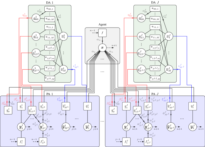
Figure 3: Factor graph representation of the joint posterior PDF (19). Short notations are used. In particular, the time index $n$ and the functional dependencies of the factors are neglected: $\bm{x}\triangleq\bm{x}_{n}$, $M^{j}\triangleq M_{n}^{(j)}$, $\underline{\bm{y}}^{j}_{s}\triangleq\underline{\bm{y}}_{s,n}^{(j)}$, $\overline{\bm{y}}^{j}_{m}\triangleq\overline{\bm{y}}_{m,n}^{(j)}$, $\underline{q}^{j}_{0}\triangleq\underline{q}_{\mathrm{P}}\big{(}\bm{x}_{n},\underline{a}^{(j)}_{00,n};\bm{z}^{(j)}_{n}\big{)}$, $\underline{q}^{j}_{s}\triangleq\underline{q}_{\mathrm{S}}\big{(}\underline{\bm{y}}_{s,n}^{(j)},\underline{a}^{(j)}_{ss,n},\bm{x}_{n};\bm{z}^{(j)}_{n}\big{)}$, $\underline{q}^{j}_{ss^{\prime}}\triangleq\underline{q}_{\text{D}}\big{(}\underline{\bm{y}}_{s,n}^{(j)},\underline{\bm{y}}_{s^{\prime},n}^{(j)},\underline{a}^{(j)}_{ss^{\prime},n},\bm{x}_{n};\bm{z}^{(j)}_{n}\big{)}{\,\underline{q}_{\text{D}}\big{(}\underline{\bm{y}}_{s^{\prime},n}^{(j)},\underline{\bm{y}}_{s,n}^{(j)},\underline{a}^{(j)}_{s^{\prime}s,n},\bm{x}_{n};\bm{z}^{(j)}_{n}\big{)}}$, $\overline{q}^{j}_{m}\triangleq\overline{q}_{\mathrm{S}}\big{(}\overline{\bm{y}}^{(j)}_{m,n},\overline{a}^{(j)}_{m,n},\bm{x}_{n};z^{(j)}_{m,n}\big{)}$, $f\triangleq f(\bm{x}_{n}|\bm{x}_{n-1})$, $f^{1}_{s}\triangleq f\big{(}\underline{\bm{y}}_{s,n}|\bm{y}_{s,n-1}\big{)}$, $f^{j}_{s}\triangleq f^{(j)}\big{(}\underline{\bm{y}}^{(j)}_{s,n}\big{|}\underline{\bm{y}}^{(j-1)}_{s,n}\big{)}$, $\alpha_{n}=\alpha(\bm{x}_{n})$, $\alpha_{s}^{j}=\alpha_{s}\big{(}\underline{\bm{y}}^{(j)}_{s,n}\big{)}$, $\beta_{ss^{\prime}}^{j}=\beta_{ss^{\prime}}\big{(}\underline{a}_{ss^{\prime},n}^{(j)}\big{)}{\,\beta_{s^{\prime}s}\big{(}\underline{a}_{s^{\prime}s,n}^{(j)}\big{)}}$, $\gamma_{ss^{\prime}}^{j}=\gamma^{(j)}_{ss^{\prime}}(\bm{x}_{n}){\,\gamma^{(j)}_{s^{\prime}s}(\bm{x}_{n})}$, $\xi_{m}^{j}=\xi\big{(}\overline{a}^{(j)}_{m,n}\big{)}$, $\eta_{ss^{\prime}}^{j}=\eta(\underline{a}_{ss^{\prime},n}^{(j)}){\,\eta(\underline{a}_{s^{\prime}s,n}^{(j)})}$, $\nu_{ss^{\prime}}^{j}=\nu_{m\rightarrow ss^{\prime}}^{(p)}(\underline{a}_{ss^{\prime},n}^{(j)}){\,\nu_{m\rightarrow s^{\prime}s}^{(p)}(\underline{a}_{s^{\prime}s,n}^{(j)})}$, $\varsigma_{m}^{j}=\varsigma\big{(}\overline{a}_{m,n}^{(j)}\big{)}$, $\zeta_{m}^{j}=\zeta_{ss^{\prime}\rightarrow m}^{(p)}\big{(}\overline{a}_{m,n}^{(j)}\big{)}{\,\zeta_{s^{\prime}s\rightarrow m}^{(p)}\big{(}\overline{a}_{m,n}^{(j)}\big{)}}$, $\tilde{\rho}_{ss^{\prime}}^{j}=\rho_{ss^{\prime}}\big{(}\underline{\bm{y}}^{(j)}_{s}\big{)}{\,\rho_{s^{\prime}s}\big{(}\underline{\bm{y}}^{(j)}_{s}\big{)}}$, and $\phi_{m}^{j}=\phi(\overline{\bm{y}}_{s}^{(j)})$. For the numbers of MVAs, the short notations reads $S^{1}\triangleq S_{n-1}$, $S^{j}\triangleq S_{n}^{(j)}$, and $(\cdot)_{S^{jj}}\triangleq(\cdot)_{S_{n}^{(j)}S_{n}^{(j)}}$. The dashed lines with arrows indicate messages representing the agent and PMVAs beliefs of time $n-1$, $n+1$ or of anchors $j-1$, $j+1$. These messages are either only sent to the next time step (e.g., from $n-1$ to $n$) or only to the next anchor (e.g., from $j-1$ to $j$).

IV Problem Formulation and Proposed Method

In this section, we formulate the estimation problem of interest and present the joint posterior PDF and factor graph underlying the proposed SLAM method.

IV-A Pre-Estimation Stage

By applying at each time $n$ a super-resolution channel estimation algorithm [18, 19, 20, 24, 21] to the observed RF signal vector one obtains, for each anchor $j$, a number of $M_{n}^{(j)}$ measurements denoted by ${\bm{z}^{(j)}_{m,n}}$ with $m\in{\cal{M}}_{n}^{(j)}\triangleq\{1,\,\dots\,,M_{n}^{(j)}\}$. Each $\bm{z}^{(j)}_{m,n}=[{z^{(j)}_{\text{d}}}_{m,n}~{}{z^{(j)}_{\varphi}}_{m,n}]^{\text{T}}$ representing a potential MPC parameter estimate contains a distance measurement ${z_{\text{d}}}_{m,n}^{(j)}\in[0,d_{\text{max}}]$ and an AOA measurement ${z_{\varphi}}_{m,n}^{(j)}\in[-\pi,\pi)$. The channel estimator decomposes the RF signal vector into individual, decorrelated components, reducing the number of dimensions (as ${M}_{n}^{(j)}$ is usually much smaller than the number of signal samples). It thus compresses the information contained in the RF signal vector into $\vspace*{-0.2mm}\bm{z}^{(j)}_{n}=[{\bm{z}^{(j)\text{T}}_{1,n}}\cdots{\bm{z}^{(j)\text{T}}_{M_{n}^{(j)},n}}]^{\text{T}}$. We also define $\bm{z}_{n}\triangleq[\bm{z}_{n}^{(1)\hskip 0.85358pt\text{T}}\dots\bm{z}_{n}^{(J)\hskip 0.85358pt\text{T}}]^{\text{T}}\vspace*{-0.6mm}$ and $\bm{z}_{1:n}\triangleq\big{[}\bm{z}^{\text{T}}_{0}\cdots\hskip 0.85358pt\bm{z}^{\text{T}}_{n}\big{]}^{\text{T}}$.

IV-B Confirmation of MVAs and State Estimation

We aim to estimate the agent state $\bm{\mathsfbr{x}}_{n}$ using all available measurements $\bm{z}_{1:n}$ from all PAs up to time $n$. In particular, we calculate an estimate $\hat{\bm{x}}_{n}$ by using the minimum mean-square error (MMSE) estimator [49, Ch. 4]

$$\hat{\bm{x}}_{n}\hskip 0.85358pt\triangleq\,\int\bm{x}_{n}\hskip 0.85358ptf(\bm{x}_{n}|\bm{z}_{1:n})\hskip 0.85358pt\mathrm{d}\bm{x}_{n}.\vspace*{-1.5mm}$$ (17)

The map of the environment is represented by reflective surfaces described by PMVAs. Therefore, the positions $\bm{\mathsfbr{p}}_{s,\mathrm{mva}}$ of the detected PMVAs $s\!\in\!\{1,\dots,S_{n}\}$ must be estimated. This relies on the marginal posterior existence probabilities $p(r_{s,n}\!=\!1|\bm{z}_{1:n})=\int f(\bm{p}_{s,\text{mva}},r_{s,n}\!=\!1|\bm{z}_{1:n})\mathrm{d}\bm{p}_{s,\text{mva}}$ and the marginal posterior PDFs $f(\bm{p}_{s,\text{mva}}|r_{s,n}\!=\!1,\bm{z}_{1:n})=f(\bm{p}_{s,\text{mva}},r_{s,n}\!=\!1|\bm{z}_{1:n})/p(r_{s,n}\!=\!1|\bm{z}_{1:n})$. A PMVA $s$ is declared to exist $p(r_{s,n}\!=\!1|\bm{z}_{1:n})>p_{\mathrm{cf}}$, where $p_{\mathrm{cf}}$ is a confirmation threshold. The number $\hat{S}_{n}$ of PMVA states that are considered to exist is the estimate of the total number $S$ of MVAs. To avoid that the number of PMVAs states grows indefinitely, PMVAs states with $p(r_{s,n}\!=\!1|\bm{z}_{1:n})<p_{\text{pr}}$ are removed from the state space (“pruned”). For existing PMVAs, an estimate of it’s position $\bm{\mathsfbr{p}}_{s,\mathrm{mva}}$ can again be calculated by the MMSE [49, Ch. 4]

$$\hat{\bm{p}}_{k,\mathrm{mva}}\,\triangleq\int\bm{p}_{k,\mathrm{mva}}\hskip 0.85358pt\hskip 0.85358ptf(\bm{p}_{k,\mathrm{mva}}\hskip 0.85358pt|\hskip 0.85358ptr_{s,n}\!=\!1,\bm{z}_{1:n})\hskip 0.85358pt\hskip 0.85358pt\mathrm{d}\bm{p}_{k,\mathrm{mva}}\hskip 0.85358pt.\vspace*{-4mm}$$ (18)

The calculation of $f(\bm{x}_{n}|\bm{z}_{1:n})$, $p(r_{s,n}\!=\!1|\bm{z})$, and $f(\bm{p}_{k,\mathrm{mva}}|$ $r_{s,n}=1,\bm{z}_{1:n})$ from the joint posterior $f(\bm{y}_{0:n},\bm{x}_{0:n},\underline{\bm{a}}_{1:n},\overline{\bm{a}}_{1:n}$ $|\hskip 0.85358pt\bm{z}_{1:n})$ by direct marginalization is not feasible. By performing sequential message passing using the SPA rules [50, 51, 43, 3] on the factor graph in Fig. 3, approximations (“beliefs”) $\tilde{f}\big{(}\bm{x}_{n}\big{)}$ and $\tilde{f}_{s}\big{(}\bm{y}_{s,n}\big{)}$ of the marginal posterior PDFs $f(\bm{x}_{n}|\bm{z}_{1:n})$, $p(r_{s,n}\!=\!1|\bm{z}_{1:n})$, and $f(\bm{p}_{s,\mathrm{mva}}|$ $r_{s,n}=1,\bm{z}_{1:n})$ can be obtained efficiently for the agent state as well as all legacy and new PMVAs states $s\in{\cal{S}}_{n}$.

$$f(\bm{y}_{0:n},\bm{x}_{0:n},\underline{\bm{a}}_{1:n},\overline{\bm{a}}_{1:n}\hskip 0.85358pt|\hskip 0.85358pt\bm{z}_{1:n})$$

$$\propto\underbrace{\bigg{(}\hskip 0.85358ptf(\bm{x}_{0})\hskip 0.85358pt\prod^{S_{0}}_{s=1}\hskip 0.85358ptf(\bm{y}_{s,0})\bigg{)}}_{\footnotesize\text{Initial prior \acsp{pdf} of \acs{pmva} and agent states}}\prod^{n}_{n^{\prime}=1}\underbrace{f\big{(}\bm{x}_{n^{\prime}}|\bm{x}_{n^{\prime}-1}\big{)}}_{\footnotesize\text{Agent state transition}}\hskip 2.27621pt\underbrace{\bigg{(}\prod^{J}_{j=1}\hskip 0.85358pt\underline{q}_{\mathrm{P}}\big{(}\bm{x}_{n^{\prime}},\underline{a}^{(j)}_{00,n^{\prime}};\bm{z}^{(j)}_{n^{\prime}}\big{)}\prod^{M^{(j)}_{n^{\prime}}}_{m^{\prime}=1}\Psi\big{(}\underline{a}^{(j)}_{00,n^{\prime}},\overline{a}^{(j)}_{m^{\prime},n^{\prime}}\big{)}\bigg{)}}_{\footnotesize\text{Factors related to \acsp{pa}}}\underbrace{\bigg{(}\prod^{S_{n^{\prime}-1}}_{s^{\prime}=1}f\big{(}\underline{\bm{y}}_{s^{\prime},n^{\prime}}|\bm{y}_{s^{\prime},n^{\prime}-1}\big{)}\bigg{)}}_{\footnotesize\text{Legacy \acs{pmva} state transition}}$$

$$\hskip 2.84526pt\times\underbrace{\bigg{(}\prod^{J}_{j^{\prime}=2}\hskip 0.85358pt\hskip 0.85358pt\bigg{(}\prod^{S^{(j^{\prime})}_{n^{\prime}}}_{s^{\prime}=1}\hskip 0.85358ptf^{(j)}\big{(}\underline{\bm{y}}^{(j^{\prime})}_{s^{\prime},n^{\prime}}\big{|}\underline{\bm{y}}^{(j^{\prime}-1)}_{s^{\prime},n^{\prime}}\big{)}\bigg{)}\bigg{)}\prod^{J}_{j=1}\bigg{(}\hskip 0.85358pt\prod^{S^{(j)}_{n^{\prime}}}_{s=1}\underline{q}_{\mathrm{S}}\big{(}\underline{\bm{y}}^{(j)}_{s,n^{\prime}},\underline{a}^{(j)}_{ss,n^{\prime}},\bm{x}_{n^{\prime}};\bm{z}^{(j)}_{n^{\prime}}\big{)}\bigg{(}\prod^{M^{(j)}_{n^{\prime}}}_{m^{\prime}=1}\Psi\big{(}\underline{a}^{(j)}_{ss,n^{\prime}},\overline{a}^{(j)}_{m^{\prime},n^{\prime}}\big{)}\bigg{)}}_{\footnotesize\text{Factors related to legacy \acs{pmva} states}}$$

$$\hskip 2.84526pt\times\underbrace{\prod^{S^{(j)}_{n^{\prime}}}_{s^{\prime}=1,s^{\prime}\neq s}\underline{q}_{\mathrm{D}}\big{(}\underline{\bm{y}}^{(j)}_{s,n^{\prime}},\underline{\bm{y}}^{(j)}_{s^{\prime},n^{\prime}},\underline{a}^{(j)}_{ss^{\prime},n^{\prime}},\bm{x}_{n^{\prime}};\bm{z}^{(j)}_{n^{\prime}}\big{)}\prod^{M^{(j)}_{n^{\prime}}}_{m^{\prime}=1}\Psi\big{(}\underline{a}^{(j)}_{ss^{\prime},n^{\prime}},\overline{a}^{(j)}_{m^{\prime},n^{\prime}}\big{)}\bigg{)}}_{\footnotesize\text{Factors related to legacy \acs{pmva} states}}\underbrace{\bigg{(}\prod^{M^{(j)}_{n^{\prime}}}_{m=1}\overline{q}_{\mathrm{S}}\big{(}\overline{\bm{y}}^{(j)}_{m,n^{\prime}},\overline{a}^{(j)}_{m,n^{\prime}},\bm{x}_{n^{\prime}};\bm{z}^{(j)}_{n^{\prime}}\big{)}\bigg{)}}_{\footnotesize\text{Prior \acsp{pdf} and related parameters of new \acs{pmva} states}}$$ (19)

IV-C The Factor Graph

By using common assumptions [44, 3], and for fixed (observed) measurements $\bm{z}_{1:n}$, the joint posterior PDF of $\bm{\mathsfbr{y}}_{0:n}$, $\bm{\mathsfbr{x}}_{0:n}$, $\underline{\bm{\mathsfbr{a}}}_{1:n}$, and $\overline{\bm{\mathsfbr{a}}}_{1:n}$, conditioned on $\bm{z}_{1:n}$ is given by (19) as shown on top of the page, where we introduced the functions $\underline{q}_{\mathrm{P}}\big{(}\bm{x}_{n^{\prime}},\underline{a}^{(j)}_{00,n^{\prime}};\bm{z}^{(j)}_{n^{\prime}}\big{)}$, $\underline{q}_{\mathrm{S}}\big{(}\underline{\bm{y}}^{(j)}_{s,n},\underline{a}^{(j)}_{ss,n},\bm{x}_{n};\bm{z}^{(j)}_{n}\big{)}$, $\underline{q}_{\mathrm{D}}\big{(}\underline{\bm{y}}^{(j)}_{s,n},\underline{\bm{y}}^{(j)}_{s^{\prime},n},\underline{a}^{(j)}_{ss^{\prime},n},\bm{x}_{n};\bm{z}^{(j)}_{n}\big{)}$, $\overline{q}_{\mathrm{S}}\big{(}\overline{\bm{y}}^{(j)}_{m,n},\overline{a}^{(j)}_{m,n},\bm{x}_{n};z^{(j)}_{m,n}\big{)}$, $\bar{f}\big{(}\overline{\bm{y}}_{s,n}\big{)}$, and $\Psi\big{(}a^{(j)}_{s,n},\overline{a}^{(j)}_{m,n}\big{)}$ that will be discussed next. A detailed derivation of (19) is provided in the supplementary material [37, Section LABEL:M-sec:app_statistical_model].

The pseudo likelihood functions of PA $j$ $\underline{q}_{\mathrm{P}}\big{(}\bm{x}_{n},\underline{a}^{(j)}_{00,n};\bm{z}^{(j)}_{n}\big{)}$, of legacy PMVAs related to single-bounce paths $\underline{q}_{\mathrm{S}}\big{(}\underline{\bm{y}}^{(j)}_{s,n},\underline{a}^{(j)}_{ss,n},\bm{x}_{n};\bm{z}^{(j)}_{n}\big{)}=\underline{q}_{\mathrm{S}}\big{(}\underline{\bm{p}}^{(j)}_{s,\mathrm{mva}},\underline{r}^{(j)}_{s,n},$ $\underline{a}^{(j)}_{ss,n},\bm{x}_{n};\bm{z}^{(j)}_{n}\big{)}$ and to double-bounce paths $\underline{q}_{\mathrm{D}}\big{(}\underline{\bm{y}}^{(j)}_{s,n},\underline{\bm{y}}^{(j)}_{s^{\prime},n},\underline{a}^{(j)}_{ss^{\prime},n},\bm{x}_{n};\bm{z}^{(j)}_{n}\big{)}=\underline{q}_{\mathrm{D}}\big{(}\underline{\bm{p}}^{(j)}_{s,\mathrm{mva}},\underline{r}^{(j)}_{s,n},\underline{\bm{p}}^{(j)}_{s^{\prime},\mathrm{mva}},$ $\underline{r}^{(j)}_{s^{\prime},n},\underline{a}^{(j)}_{ss^{\prime},n},\bm{x}_{n};\bm{z}^{(j)}_{n}\big{)}\vspace*{0.4mm}$ are, respectively, given for $(0,0)$ by

$$\underline{q}_{\mathrm{P}}\big{(}\bm{x}_{n},\underline{a}^{(j)}_{00,n};\bm{z}^{(j)}_{n}\big{)}$$

$$\hskip 11.38109pt\triangleq\begin{cases}\displaystyle\hskip 0.85358pt\frac{p^{(j)}_{\mathrm{d}}(\bm{p}_{n})f\big{(}\bm{z}_{m,n}^{(j)}\big{|}\hskip 0.85358pt\bm{p}_{n}\big{)}}{\mu_{\mathrm{fp}}\hskip 0.85358ptf_{\mathrm{fp}}\big{(}\bm{z}_{m,n}^{(j)}\big{)}}\hskip 0.85358pt,&\!\!\underline{a}^{(j)}_{00,n}\!=m\in{\cal{M}}_{n}^{(j)}\\[9.95845pt] 1\!-p^{(j)}_{\mathrm{d}}(\bm{p}_{n})\hskip 0.85358pt,&\!\!\underline{a}^{(j)}_{00,n}\!=0\end{cases}$$ (20)

for $(s,s)\in\mathcal{D}^{(j)}_{\text{S},n}$ by

$$\underline{q}_{\mathrm{S}}\big{(}\underline{\bm{p}}^{(j)}_{s,\mathrm{mva}},\underline{r}^{(j)}_{s,n}=1,\underline{a}^{(j)}_{ss,n},\bm{x}_{n};\bm{z}^{(j)}_{n}\big{)}$$

$$\triangleq\begin{cases}\displaystyle\hskip 0.85358pt\frac{p^{(j)}_{\mathrm{d}}(\bm{p}_{n},\bm{p}^{(j)}_{s,\text{mva}})f\big{(}\bm{z}_{m,n}^{(j)}\big{|}\hskip 0.85358pt\bm{p}_{n},\bm{p}_{s,\text{mva}}^{(j)}\big{)}}{\mu_{\mathrm{fp}}\hskip 0.85358ptf_{\mathrm{fp}}\big{(}\bm{z}_{m,n}^{(j)}\big{)}}\hskip 0.85358pt,&\!\!\underline{a}^{(j)}_{ss,n}\!=m\in{\cal{M}}_{n}^{(j)}\\[9.95845pt] 1\!-p^{(j)}_{\mathrm{d}}(\bm{p}_{n},\bm{p}^{(j)}_{s,\text{mva}})\hskip 0.85358pt,&\!\!\underline{a}^{(j)}_{ss,n}\!=0\end{cases}$$ (21)

and $\underline{q}_{\mathrm{S}}\big{(}\underline{\bm{p}}^{(j)}_{s,\mathrm{mva}},\underline{r}^{(j)}_{s,n}=0,\underline{a}^{(j)}_{ss,n},\bm{x}_{n};\bm{z}^{(j)}_{n}\big{)}\triangleq{\delta_{\underline{a}^{(j)}_{ss,n}}}$ as well as for $(s,s^{\prime})\in\mathcal{D}^{(j)}_{\text{D},n}$ by

$$\underline{q}_{\mathrm{D}}\big{(}\underline{\bm{p}}^{(j)}_{s,\mathrm{mva}},\underline{r}^{(j)}_{s,n}=1,\underline{\bm{p}}^{(j)}_{s^{\prime},\mathrm{mva}},\underline{r}^{(j)}_{s^{\prime},n}=1,\underline{a}^{(j)}_{ss^{\prime},n},\bm{x}_{n};\bm{z}^{(j)}_{n}\big{)}$$

$$\triangleq\begin{cases}\displaystyle\hskip 0.85358pt\frac{p^{(j)}_{\mathrm{d}}(\bm{p}_{n},\bm{p}^{(j)}_{s,\text{mva}},\bm{p}^{(j)}_{s^{\prime},\text{mva}})}{\mu_{\mathrm{fp}}}\\[8.53581pt] \hskip 11.38109pt\times\frac{f(\bm{z}_{m,n}^{(j)}|\hskip 0.85358pt\bm{p}_{n},\underline{\bm{p}}^{(j)}_{s,\mathrm{mva}},\underline{\bm{p}}^{(j)}_{s^{\prime},\mathrm{mva}})}{f_{\mathrm{fp}}(\bm{z}_{m,n}^{(j)})}\hskip 0.85358pt,\hskip 2.84526pt&\!\!a^{(j)}_{ss^{\prime}}\!=m\in{\cal{M}}_{n}^{(j)}\\[9.95845pt] 1\!-p^{(j)}_{\mathrm{d}}(\bm{p}_{n},\bm{p}^{(j)}_{s,\text{mva}},\bm{p}^{(j)}_{s^{\prime},\text{mva}})\hskip 0.85358pt,\hskip 2.84526pt&\!\!a^{(j)}_{ss^{\prime}}\!=0\end{cases}$$ (22)

and $\underline{q}_{\mathrm{D}}\big{(}\underline{\bm{p}}^{(j)}_{s,\mathrm{mva}},\underline{r}^{(j)}_{s,n},\underline{\bm{p}}^{(j)}_{s^{\prime},\mathrm{mva}},\underline{r}^{(j)}_{s^{\prime},n},\underline{a}^{(j)}_{ss^{\prime},n},\bm{x}_{n};\bm{z}^{(j)}_{n}\big{)}\triangleq\delta_{\underline{a}^{(j)}_{ss^{\prime},n}}$ if any $\underline{r}^{(j)}_{s^{\prime\prime},n}=0$ for $s^{\prime\prime}\in\{s,s^{\prime}\}$.

The pseudo likelihood functions related to new PMVAs $\overline{q}_{\mathrm{S}}\big{(}\overline{\bm{y}}^{(j)}_{m,\mathrm{mva}},\overline{a}^{(j)}_{m,n},\bm{x}_{n};\bm{z}^{(j)}_{n}\big{)}=\overline{q}_{\mathrm{S}}\big{(}\overline{\bm{p}}^{(j)}_{m,\mathrm{mva}},\overline{r}^{(j)}_{s,n},\overline{a}^{(j)}_{m,n},\bm{x}_{n};\bm{z}^{(j)}_{n}\big{)}$ is given by

$$\overline{q}_{\mathrm{S}}\big{(}\overline{\bm{p}}^{(j)}_{m,\mathrm{mva}},\overline{r}^{(j)}_{s,n}=1,\overline{a}^{(j)}_{m,n},\bm{x}_{n};\bm{z}^{(j)}_{n}\big{)}$$

$$\triangleq\begin{cases}0\hskip 0.85358pt,&\overline{a}^{(j)}_{m,n}\in\tilde{{\cal{D}}}_{n}^{(j)}\\[2.84526pt] \frac{\mu_{\mathrm{n}}f_{\mathrm{n}}(\overline{\bm{p}}^{(j)}_{m,\mathrm{mva}}\hskip 0.85358pt|\hskip 0.85358pt\bm{p}_{n})f(\bm{z}_{m,n}^{(j)}\hskip 0.85358pt|\bm{p}_{n},\overline{\bm{p}}^{(j)}_{m,\mathrm{mva}})}{\mu_{\mathrm{fp}}f_{\mathrm{fp}}(\bm{z}_{m,n}^{(j)})}\hskip 0.85358pt,&\overline{a}^{(j)}_{m,n}=0\end{cases}$$ (23)

and $\overline{q}_{\mathrm{S}}\big{(}\overline{\bm{p}}^{(j)}_{m,\mathrm{mva}},\overline{r}^{(j)}_{s,n}=0,\overline{a}^{(j)}_{m,n},\bm{x}_{n};z^{(j)}_{m,n}\big{)}\triangleq f_{\text{d}}\big{(}\overline{\bm{p}}^{(j)}_{m,\mathrm{mva}}\big{)}$, respectively. Note that the first line in (23) is zero because per definition, the new PMVA with index $m$ exists ($\overline{r}_{m,n}=1$) if and only if the measurement is not associated to a legacy PMVA. For $\overline{a}^{(j)}_{m,n}=0$, for each measurement $z^{(j)}_{m,n}$ a new PMVA is introduced, implying that each measurement $\bm{z}_{m,n}^{(j)}$ is assumed to originate from a single-bounce path corresponding to exactly one PMVA $s\in{\cal{M}}_{n}^{(j)}$ (not a pair of PMVAs).

Finally, the binary check functions that validates consistency for any pair $(\mathsfbr{\underline{a}}^{(j)}_{ss^{\prime},n},\overline{\mathsfbr{a}}^{(j)}_{m,n})$ of PMVA-oriented and measurement-oriented association variable at time $n$, read

$$\Psi(\underline{a}^{(j)}_{ss^{\prime},n},\overline{a}^{(j)}_{m,n})\hskip 5.69054pt\triangleq\begin{cases}0,&\begin{minipage}{142.26378pt} $\underline{a}^{(j)}_{ss^{\prime},n}=m,\overline{a}^{(j)}_{m,n}\neq(s,s^{\prime})\text{ or }\\ \underline{a}^{(j)}_{ss^{\prime},n}\neq m,\overline{a}^{(j)}_{m,n}=(s,s^{\prime})$ \end{minipage}\\[0.28453pt] 1\hskip 0.85358pt,&\text{otherwise}.\end{cases}$$

In case the joint PMVA-oriented association vector $\underline{\bm{\mathsfbr{a}}}_{n}$ and the measurement-oriented association vector $\overline{\bm{\mathsfbr{a}}}_{n}$ do not describe the same association event, at least one check function in (19) is zero. Thus $f(\bm{y}_{0:n},\bm{x}_{0:n},\underline{\bm{a}}_{1:n},\overline{\bm{a}}_{1:n}\hskip 0.85358pt|\hskip 0.85358pt\bm{z}_{1:n})$ is zero as well. The factor graph representing factorization (19) is shown in Fig. 3. A detailed derivation of related factorization structures developed in the context of multitarget tracking and their relationship to the TOMB/P filter is presented in [44]. The problem and resulting factorization structure considered in this paper are more complicated than multisensor multitarget tracking because (i) there is also an unknown agent state and (ii) measurements can originate from two different types of propagation paths.

V Proposed Sum-Product Algorithm

Since our factor graph in Fig. 3 has cycles, we have to decide on a specific order of message computation [50, 52]. We choose the order according to the following rules [3, 5, 25, 24, 43, 44, 51]: (i) messages are only sent forward in time; (ii) messages are only sent from PA $j-1$ to PA $j$, i.e., the measurements of PA are processed serial, thus, PA $j-1$ establishes new PMVAs that are acting as legacy PMVAs for PA $j$; (iii) iterative message passing is only performed for data association [3, 4], i.e., in particular, for the loops connecting different PMVAs, we only perform a single message passing iteration; and (iv) along an edge connecting an agent state variable node and a new PMVA state variable node, messages are only sent from the former to the latter. With these rules, the message passing equations of the SPA [50] yield the following operations at each time step. The corresponding messages are shown in Fig. 3. Note that this message passing order has been developed for real-time processing. Sending messages also backward in time, referred to as “smoothing,” will improve post-processing performance but lead to increased computational complexity.

We note that similarly to the “dummy PDFs” introduced in Section III, we consider messages $\varphi\big{(}\bm{y}_{s,n}\big{)}=\varphi\big{(}\bm{p}_{s,\mathrm{mva}}\hskip 0.85358pt,r_{s,n}\big{)}$ for non-existing PMVA states, i.e., for $r_{s,n}\!=0$. We define these messages by $\varphi\big{(}\bm{p}_{s,\mathrm{mva}}\hskip 0.85358pt,0\big{)}\triangleq\varphi^{(j)}_{k,n}$ (note that these messages are not PDFs and thus are not required to integrate to $1$). To keep the notation concise, we also define the sets ${\cal{M}}_{0,n}^{(j)}\triangleq{\cal{M}}_{n}^{(j)}\cup\{0\}$ and $\tilde{{\cal{D}}}^{(j)}_{0,n}\in\tilde{{\cal{D}}}^{(j)}_{n}\cup\{0\}$.

V-A Prediction Step

First, a prediction step is performed for the agent and all legacy PMVAs $s\in S_{n-1}$. Based on the SPA rule, the prediction message for the agent state is given by

$$\alpha(\bm{x}_{n})=\int f(\bm{x}_{n}|\bm{x}_{n-1})\hskip 0.85358pt\tilde{f}(\bm{x}_{n-1})\hskip 0.85358pt\mathrm{d}\bm{x}_{n-1}$$ (24)

and the prediction message for the legacy PMVAs is given by

$$\alpha_{s}\big{(}\underline{\bm{p}}_{s,\text{mva}}\hskip 0.85358pt,\underline{r}_{s,n}\big{)} =\sum_{r_{k,n-1}\in\{0,1\}}\int f\big{(}\underline{\bm{p}}_{s,\text{mva}}\hskip 0.85358pt,\underline{r}_{s,n}\big{|}\bm{p}_{s,\text{mva}}\hskip 0.85358pt,r_{s,n-1}\big{)}$$

$$\hskip 14.22636pt\times\tilde{f}\big{(}\bm{p}_{s,\text{mva}}\hskip 0.85358pt,r_{s,n-1}\big{)}\hskip 0.85358pt\mathrm{d}\bm{p}_{s,\text{mva}}$$ (25)

$s\in\{1,\dots,S_{n-1}\}$, where the beliefs of the agent state, $\tilde{f}(\bm{x}_{n-1})$, and of the PMVA states, $\tilde{f}\big{(}\bm{p}_{s,\text{mva}}\hskip 0.85358pt,r_{s,n-1}\big{)}$, were calculated at the preceding time $n-1$. Inserting (8) and (9) for $f\big{(}\underline{\bm{p}}_{s,\text{mva}}\hskip 0.85358pt,\underline{r}_{s,n}\big{|}\bm{p}_{s,\text{mva}}\hskip 0.85358pt,r_{s,n-1}=1\big{)}$ and $f\big{(}\underline{\bm{p}}_{s,\text{mva}}\hskip 0.85358pt,\underline{r}_{s,n}\big{|}\bm{p}_{s,\text{mva}}\hskip 0.85358pt,$$r_{s,n-1}=0\big{)}$, respectively, we obtain

$$\alpha_{s}\big{(}\underline{\bm{p}}_{s,\text{mva}}\hskip 0.85358pt,1\big{)}=\hskip 0.85358ptp_{\text{s}}\int\delta\big{(}\underline{\bm{p}}_{s,\text{mva}}-\bm{p}_{s,\text{mva}}\big{)}\hskip 0.85358pt\tilde{f}_{s}\big{(}\bm{p}_{s,\text{mva}}\hskip 0.85358pt,1\big{)}\hskip 0.85358pt\mathrm{d}\bm{p}_{s,\text{mva}}$$ (26)

and $\alpha_{s}\big{(}\underline{\bm{p}}_{s,\text{mva}}\hskip 0.85358pt,0\big{)}=\alpha_{s,n}f_{\text{d}}\big{(}\bm{p}_{s,\mathrm{mva}}\big{)}$ with

$$\alpha_{s,n}=(1\!-p_{\text{s}}\big{)}\int\tilde{f}_{s}\big{(}\bm{p}_{s,\text{mva}}\hskip 0.85358pt,1\big{)}\hskip 0.85358pt\mathrm{d}\bm{p}_{s,\text{mva}}+\hskip 0.85358pt\tilde{f}_{s,n-1}\hskip 0.85358pt.$$ (27)

We note that $\tilde{f}_{s,n-1}\triangleq\int\tilde{f}_{s}\big{(}\bm{p}_{s,\text{mva}}\hskip 0.85358pt,0\big{)}\hskip 0.85358pt\mathrm{d}\bm{p}_{s,\text{mva}}$ approximates the probability of non-existence of legacy PMVA $s$ at the previous time step $n-1$.

V-B Sequential PA Update

At iteration $j\in\{1,\dots,J\}$, the following operations are calculated for all legacy and new PMVAs.

V-B1 Transition of New and Legacy PMVA States Between PAs

For $j=1$, the number of legacy PMVAs is $S^{(1)}_{n}=S_{n-1}$ with the corresponding state $\underline{\bm{y}}^{(1)}_{n}\triangleq\big{[}\underline{\bm{y}}^{\text{T}}_{1,n}\cdots\hskip 0.85358pt\underline{\bm{y}}^{T}_{S_{n-1},n}\big{]}^{\text{T}}$. Furthermore, the state $\overline{\bm{y}}^{(j-1)}$ is empty and the prediction message of legacy PMVAs is $\alpha_{s}\big{(}\underline{\bm{p}}^{(j)}_{s,\text{mva}}\hskip 0.85358pt,\underline{r}_{s,n}\big{)}\triangleq\alpha_{s}\big{(}\underline{\bm{p}}_{s,\text{mva}}\hskip 0.85358pt,\underline{r}_{s,n}\big{)}$ as well as $\alpha^{(j)}_{s,n}\triangleq\alpha_{s,n}$. For $j>1$, we have $S^{(j)}_{n}=S^{(j-1)}_{n}+M^{(j-1)}_{n}$ legacy PMVAs with states $\underline{\bm{y}}^{(j)}_{n}=\big{[}\underline{\bm{y}}^{(j-1)\text{T}}_{n}\hskip 0.85358pt\hskip 0.85358pt\hskip 0.85358pt\overline{\bm{y}}^{(j-1)\text{T}}_{n}\big{]}^{\text{T}}$ and $M^{(j)}_{n}$ new PMVAs with states $\overline{\bm{y}}^{(j)}$. For $1\leqslant s\leqslant S^{(j-1)}_{n}$, using (10), (11), and (25) the prediction message of former legacy PMVAs is given by

$$\alpha_{s}\big{(}\underline{\bm{p}}^{(j)}_{s,\text{mva}}\hskip 0.85358pt,1\big{)}=\int\delta\big{(}\underline{\bm{p}}^{(j)}_{s,\text{mva}}-\bm{p}^{(j-1)}_{s,\text{mva}}\big{)}\hskip 0.85358pt\gamma\big{(}\underline{\bm{p}}^{(j-1)}_{s,\mathrm{mva}},1\big{)}\hskip 0.85358pt\mathrm{d}\bm{p}^{(j-1)}_{s,\text{mva}}\vspace{1.2mm}$$ (28)

and $\alpha_{s}\big{(}\underline{\bm{p}}^{(j)}_{s,\text{mva}}\hskip 0.85358pt,0\big{)}=\alpha^{(j)}_{s,n}f_{\text{d}}\big{(}\underline{\bm{p}}^{(j)}_{s,\mathrm{mva}}\big{)}$ with $\alpha^{(j)}_{s,n}=\gamma_{s,n}^{(j-1)}$. The prediction message of former new PMVAs is $\alpha_{s}\big{(}\underline{\bm{p}}^{(j)}_{s,\text{mva}}\hskip 0.85358pt,\underline{r}_{s,n}\big{)}\triangleq\phi\big{(}\overline{\bm{y}}^{(j)}_{s,n}\big{)}$ and $\alpha^{(j)}_{s,n}\triangleq\phi^{(j)}_{s,n}$.

V-B2 Checking the Availability of Propagation Paths

The proposed SPA algorithm performs an availability check for each propagation path using RT [34, 35, 36] to determine whether a VA can provide map information. First, the VA positions $\bm{p}^{(j)}_{ss^{\prime},\text{va}}$ are determined by applying (3) directly to PA $j$ at position $\bm{p}^{(j)}_{\text{pa}}$ to get single-bounce-related VAs at positions $\bm{p}^{(j)}_{ss,\text{va}}$. Next, (3) is also applied to this single-bounce-related VAs to get double-bounce-related VAs at positions $\bm{p}^{(j)}_{ss^{\prime},\text{va}}$. rt is performed as described in Section III-D. In case the path between the agent position and a VA position or between two VA positions (double-bounce path) intersects with a reflective surface (e.g., it is blocked), the corresponding path is not available at $\bm{p}_{n}$. Hence, the corresponding VA cannot be associated with measurements at time $n$.

V-B3 Measurement Evaluation for the LOS Path

The messages $\beta_{00}\big{(}\underline{a}^{(j)}_{00,n}\big{)}$ passed from the factor node $\underline{q}_{\mathrm{P}}\big{(}\bm{x}_{n},\underline{a}^{(j)}_{00,n};\bm{z}^{(j)}_{n}\big{)}$ to the feature-oriented association variables $\underline{a}^{(j)}_{00,n}$ are calculated as

$$\beta_{00}\big{(}\underline{a}^{(j)}_{00,n}\big{)} =\int\alpha(\bm{x}_{n})\hskip 0.85358pt\underline{q}_{\mathrm{P}}\big{(}\bm{x}_{n},\underline{a}^{(j)}_{00,n};\bm{z}^{(j)}_{n}\big{)}\mathrm{d}\bm{x}_{n}\hskip 0.85358pt.$$ (29)

V-B4 Measurement Evaluation for Legacy PMVAs

For $s=s^{\prime}$, the messages $\beta_{ss}\big{(}\underline{a}_{ss,n}^{(j)}\big{)}$ passed from the factor node $\underline{q}_{\mathrm{S}}\big{(}\underline{\bm{p}}^{(j)}_{s,\mathrm{mva}},\underline{r}^{(j)}_{s,n},\underline{a}^{(j)}_{ss,n},\bm{x}_{n};\bm{z}^{(j)}_{n}\big{)}$ of single PMVAs to the feature-oriented association variables $a_{ss,n}^{(j)}$ given by

$$\beta_{ss}\big{(}\underline{a}_{ss,n}^{(j)}\big{)}$$

$$=\int\!\!\!\int\alpha_{s}\big{(}\underline{\bm{p}}_{s,\text{mva}}^{(j)},1\big{)}\hskip 0.85358pt\alpha(\bm{x}_{n})\underline{q}_{\mathrm{S}}\big{(}\underline{\bm{p}}^{(j)}_{s,\mathrm{mva}},\underline{r}^{(j)}_{s,n},\underline{a}^{(j)}_{ss,n},\bm{x}_{n};\bm{z}^{(j)}_{n}\big{)}$$

$$\hskip 14.22636pt\times\mathrm{d}\bm{x}_{n}\hskip 0.85358pt\mathrm{d}\underline{\bm{p}}_{s,\text{mva}}^{(j)}\hskip 0.85358pt+\hskip 0.85358pt1\big{(}\underline{a}_{ss,n}^{(j)}\big{)}\hskip 0.85358pt\alpha_{s,n}^{(j)}\hskip 0.85358pt.$$ (30)

For $s\neq s^{\prime}$, the message $\beta_{ss^{\prime}}\big{(}\underline{a}_{ss^{\prime},n}^{(j)}\big{)}$ passed from the factor node $\underline{q}_{\mathrm{D}}\big{(}\underline{\bm{p}}^{(j)}_{s,\mathrm{mva}},\underline{r}^{(j)}_{s,n},\underline{\bm{p}}^{(j)}_{s^{\prime},\mathrm{mva}},\underline{r}^{(j)}_{s^{\prime},n},\underline{a}^{(j)}_{ss^{\prime},n},\bm{x}_{n};\bm{z}^{(j)}_{n}\big{)}$ of pairs of PMVAs to the feature-oriented association variables $a_{ss^{\prime},n}^{(j)}$ are obtained as

$$\beta_{ss^{\prime}}\big{(}\underline{a}_{ss^{\prime},n}^{(j)}\big{)} =\int\!\!\!\int\!\!\!\int\alpha_{s}\big{(}\underline{\bm{p}}_{s,\text{mva}}^{(j)},1\big{)}\hskip 0.85358pt\alpha_{s}\big{(}\underline{\bm{p}}_{s^{\prime},\text{mva}}^{(j)},1\big{)}\alpha(\bm{x}_{n})$$

$$\times\underline{q}_{\mathrm{D}}\big{(}\underline{\bm{p}}^{(j)}_{s,\mathrm{mva}},\underline{r}^{(j)}_{s,n},\underline{\bm{p}}^{(j)}_{s^{\prime},\mathrm{mva}},\underline{r}^{(j)}_{s^{\prime},n},\underline{a}^{(j)}_{ss^{\prime},n},\bm{x}_{n};\bm{z}^{(j)}_{n}\big{)}$$

$$\times\mathrm{d}\bm{x}_{n}\hskip 0.85358pt\mathrm{d}\underline{\bm{p}}_{s,\text{mva}}^{(j)}\mathrm{d}\underline{\bm{p}}_{s^{\prime},\text{mva}}^{(j)}+1\big{(}\underline{a}_{ss^{\prime},n}^{(j)}\big{)}\hskip 0.85358pt\alpha_{s,n}^{(j)}\alpha_{s^{\prime},n}^{(j)}\hskip 0.85358pt.$$ (31)

V-B5 Measurement Evaluation for New PMVAs

For PA $j$, the messages $\xi\big{(}\overline{a}^{(j)}_{m,n}\big{)}$ sent from the factor node $\overline{q}_{\mathrm{S}}\big{(}\overline{\bm{p}}^{(j)}_{m,\mathrm{mva}},\overline{r}^{(j)}_{k,\mathrm{mva}},\overline{a}^{(j)}_{m,n},\bm{x}_{n};z^{(j)}_{m,n}\big{)}$ to the variable nodes corresponding to the measurement-oriented association variables $\overline{a}^{(j)}_{m,n}$ are given by

$$\xi\big{(}\overline{a}^{(j)}_{m,n}\big{)} =\sum_{\overline{r}^{(j)}_{m,n}\in\{0,1\}}\int\!\!\!\int\overline{q}_{\mathrm{S}}\big{(}\overline{\bm{p}}^{(j)}_{m,\mathrm{mva}},\overline{r}^{(j)}_{k,\mathrm{mva}},\overline{a}^{(j)}_{m,n},\bm{x}_{n};z^{(j)}_{m,n}\big{)}$$

$$\hskip 14.22636pt\times\alpha(\bm{x}_{n})\,\mathrm{d}\bm{x}_{n}\hskip 0.85358pt\mathrm{d}\overline{\bm{p}}^{(j)}_{m,\mathrm{mva}}\hskip 0.85358pt.$$ (32)

Using the expression of $\overline{q}_{\mathrm{S}}\big{(}\overline{\bm{p}}^{(j)}_{m,\mathrm{mva}},\overline{r}^{(j)}_{k,\mathrm{mva}},\overline{a}^{(j)}_{m,n},\bm{x}_{n};z^{(j)}_{m,n}\big{)}$ in Section IV-C in (23), Eq. (32) simplifies to $\xi\big{(}\overline{a}^{(j)}_{m,n}\big{)}\!=\!1$ for $\overline{a}^{(j)}_{m,n}\!\in\!{\cal{D}}^{(j)}_{n}$, and for $\overline{a}^{(j)}_{m,n}\!=0$ it becomes

$$\xi\big{(}\overline{a}^{(j)}_{m,n}\big{)} =1+\frac{\mu_{\text{n}}}{\mu_{\text{fp}}\hskip 0.85358ptf_{\text{fp}}\big{(}\bm{z}^{(j)}_{m,n}\big{)}}\int\!\!\!\int\alpha(\bm{x}_{n})\hskip 0.85358ptf_{\text{n}}\big{(}\overline{\bm{p}}^{(j)}_{m,\mathrm{mva}}\big{|}\bm{x}_{n}\big{)}$$

$$\hskip 14.22636pt\times f\big{(}\bm{z}^{(j)}_{m,n}\big{|}\bm{x}_{n},\overline{\bm{p}}^{(j)}_{m,\mathrm{mva}}\big{)}\,\mathrm{d}\bm{x}_{n}\hskip 0.85358pt\mathrm{d}\overline{\bm{p}}^{(j)}_{m,\mathrm{mva}}\hskip 0.85358pt.$$ (33)

V-B6 Iterative Data Association

Next, from $\beta\big{(}\underline{a}_{ss^{\prime},n}^{(j)}\big{)}$ and $\xi\big{(}\overline{a}^{(j)}_{m,n}\big{)}$, messages $\eta\big{(}\underline{a}_{ss^{\prime},n}^{(j)}\big{)}$ and $\varsigma\big{(}\overline{a}_{m,n}^{(j)}\big{)}$ are obtained using loopy (iterative) BP. First, for each measurement, $m\!\in\!{\cal{M}}_{n}^{(j)}$, messages $\nu_{m\rightarrow s}^{(p)}\big{(}\underline{a}_{ss^{\prime},n}^{(j)}\big{)}$ and, then, for $ss^{\prime}\in\tilde{\mathcal{D}}_{n}^{(j)}$ messages $\zeta_{s\rightarrow m}^{(p)}\big{(}\overline{a}_{m,n}^{(j)}\big{)}$ are calculated iteratively according to [47, 44], for each iteration index $p\in\{1,\ldots,P\}$. After the last iteration $p=P$, the messages $\eta\big{(}\underline{a}_{ss^{\prime},n}^{(j)}\big{)}$ and $\varsigma\big{(}\overline{a}_{m,n}^{(j)}\big{)}$ are calculated according to [47, 44]. Details are provided in the supplementary material[37, Section LABEL:M-sec:DA].

V-B7 Measurement Update for the Agent

The message $\gamma^{(j)}_{00}(\bm{x}_{n})$ sent from the factor node $\underline{q}_{\mathrm{P}}\big{(}\bm{x}_{n},\underline{a}^{(j)}_{00,n};\bm{z}^{(j)}_{n}\big{)}$ to the agent variable node is computed as

$$\gamma^{(j)}_{00}(\bm{x}_{n}) =\!\sum_{\underline{a}^{(j)}_{00,n}\in{\cal{M}}_{0,n}^{(j)}}\!\!\eta\big{(}\underline{a}^{(j)}_{00,n}\big{)}\underline{q}_{\mathrm{P}}\big{(}\bm{x}_{n},\underline{a}^{(j)}_{00,n};\bm{z}^{(j)}_{n}\big{)}\hskip 0.85358pt.$$ (34)

For $s=s^{\prime}$, the messages $\gamma^{(j)}_{ss}(\bm{x}_{n})$ sent from the factor node $\underline{q}_{\mathrm{S}}\big{(}\underline{\bm{p}}^{(j)}_{s,\mathrm{mva}},1,\underline{a}^{(j)}_{ss,n},\bm{x}_{n};\bm{z}^{(j)}_{n}\big{)}$ to the agent variable node are given by

$$\gamma^{(j)}_{ss}(\bm{x}_{n}) =\sum_{a_{ss,n}^{(j)}\in{\cal{M}}_{0,n}^{(j)}}\!\!\eta\big{(}\underline{a}_{ss,n}^{(j)}\big{)}\int\!\underline{q}_{\mathrm{S}}\big{(}\underline{\bm{p}}^{(j)}_{s,\mathrm{mva}},1,\underline{a}^{(j)}_{ss,n},\bm{x}_{n};\bm{z}^{(j)}_{n}\big{)}$$

$$\hskip 5.69054pt\times\alpha_{s}\big{(}\underline{\bm{p}}_{s,\text{mva}}^{(j)},1\big{)}\mathrm{d}\underline{\bm{p}}_{s,\text{mva}}^{(j)}\hskip 0.85358pt+\hskip 0.85358pt\eta\big{(}\underline{a}_{ss,n}^{(j)}\!=\!0\big{)}\hskip 0.85358pt\alpha_{s,n}^{(j)}.$$ (35)

Furthermore, for $s\neq s^{\prime}$, the messages passed from the factor node $\underline{q}_{\mathrm{D}}\big{(}\underline{\bm{p}}^{(j)}_{s,\mathrm{mva}},1,\underline{\bm{p}}^{(j)}_{s^{\prime},\mathrm{mva}},1,$ $\underline{a}^{(j)}_{ss^{\prime},n},\bm{x}_{n};\bm{z}^{(j)}_{n}\big{)}$ to the agent variable node are obtained as

$$\gamma^{(j)}_{ss^{\prime}}(\bm{x}_{n}) =\!\!\!\!\sum_{\underline{a}_{ss^{\prime},n}^{(j)}\in{\cal{M}}_{0,n}^{(j)}}\!\!\!\!\!\eta\big{(}\underline{a}_{ss^{\prime},n}^{(j)}\big{)}\int\!\!\!\!\int\!\!\alpha_{s}\big{(}\underline{\bm{p}}_{s,\text{mva}}^{(j)},1\big{)}\alpha_{s^{\prime}}\big{(}\underline{\bm{p}}_{s^{\prime},\text{mva}}^{(j)},1\big{)}$$

$$\hskip 5.69054pt\times\!\underline{q}_{\mathrm{D}}\big{(}\underline{\bm{p}}^{(j)}_{s,\mathrm{mva}},1,\underline{\bm{p}}^{(j)}_{s^{\prime},\mathrm{mva}},1,\underline{a}^{(j)}_{ss^{\prime},n},\bm{x}_{n};\bm{z}^{(j)}_{n}\big{)}$$

$$\hskip 5.69054pt\times\mathrm{d}\underline{\bm{p}}_{s,\text{mva}}^{(j)}\mathrm{d}\underline{\bm{p}}_{s^{\prime},\text{mva}}^{(j)}\hskip 0.85358pt+\hskip 0.85358pt\eta\big{(}\underline{a}_{ss^{\prime},n}^{(j)}\!=\!0\big{)}\hskip 0.85358pt\alpha_{s,n}^{(j)}\hskip 0.85358pt\alpha_{s^{\prime},n}^{(j)}\hskip 0.85358pt.$$ (36)

V-B8 Measurement Update for Legacy PMVAs

Similarly, for $s=s^{\prime}$, the messages $\rho_{ss^{\prime}}\big{(}\underline{\bm{y}}^{(j)}_{s}\big{)}$ sent to the legacy PMVAs variable nodes are given by

$$\rho_{ss}\big{(}\underline{\bm{p}}^{(j)}_{s,\mathrm{mva}},1\big{)} =\sum_{\underline{a}_{ss,n}^{(j)}\in{\cal{M}}_{0,n}^{(j)}}\int\!\!\eta\big{(}\underline{a}_{ss,n}^{(j)}\big{)}\alpha(\bm{x}_{n})$$

$$\hskip 5.69054pt\times\!\underline{q}_{\mathrm{S}}\big{(}\underline{\bm{p}}^{(j)}_{s,\mathrm{mva}},1,\underline{a}^{(j)}_{ss,n},\bm{x}_{n};\bm{z}^{(j)}_{n}\big{)}\mathrm{d}\bm{x}_{n}$$ (37)

$$\rho_{ss}^{(j)} \triangleq\rho_{ss}\big{(}\underline{\bm{p}}^{(j)}_{s,\mathrm{mva}},0\big{)}=\eta\big{(}\underline{a}_{ss,n}^{(j)}\!=\!0\big{)}$$ (38)

and for $s\neq s^{\prime}$ by

$$\rho_{ss^{\prime}}\big{(}\underline{\bm{p}}^{(j)}_{s,\mathrm{mva}},1\big{)} =\sum_{\underline{a}_{ss^{\prime},n}^{(j)}\in{\cal{M}}_{0,n}^{(j)}}\int\int\eta\big{(}\underline{a}_{ss^{\prime},n}^{(j)}\big{)}\alpha(\bm{x}_{n})\alpha_{s^{\prime}}\big{(}\underline{\bm{p}}_{s^{\prime},\text{mva}}^{(j)},1\big{)}$$

$$\times\!\underline{q}_{\mathrm{D}}\big{(}\underline{\bm{p}}^{(j)}_{s,\mathrm{mva}},1,\underline{\bm{p}}^{(j)}_{s^{\prime},\mathrm{mva}},1,\underline{a}^{(j)}_{ss^{\prime},n},\bm{x}_{n};\bm{z}^{(j)}_{n}\big{)}$$

$$\times\mathrm{d}\bm{x}_{n}\mathrm{d}\underline{\bm{p}}_{s^{\prime},\text{mva}}^{(j)}$$ (39)

$$\rho_{ss^{\prime}}^{(j)} \triangleq\rho_{ss^{\prime}}\big{(}\underline{\bm{p}}^{(j)}_{s,\mathrm{mva}},0\big{)}=\eta\big{(}\underline{a}_{ss^{\prime},n}^{(j)}\!=\!0\big{)}\hskip 0.85358pt.$$ (40)

Based on these messages, the message sent to the next PA $\gamma\big{(}\underline{\bm{y}}_{s}^{(j)}\big{)}\triangleq\gamma\big{(}\underline{\bm{p}}_{s,\text{mva}}^{(j)},\underline{r}_{k,n}^{(j)}\big{)}$ is computed as

$$\gamma\big{(}\underline{\bm{p}}^{(j)}_{s,\mathrm{mva}},1\big{)} =\!\rho_{ss}\big{(}\underline{\bm{p}}^{(j)}_{s,\mathrm{mva}},1\big{)}+\prod^{S_{n}^{(j)}}_{s^{\prime}=1,s\neq s^{\prime}}\rho_{ss^{\prime}}\big{(}\underline{\bm{p}}^{(j)}_{s,\mathrm{mva}},1\big{)}$$ (41)

$$\gamma_{s,n}^{(j)} \triangleq\hskip 0.85358pt\gamma\big{(}\underline{\bm{p}}^{(j)}_{s,\mathrm{mva}},0\big{)}=\rho_{ss}^{(j)}+\prod^{S_{n}^{(j)}}_{s^{\prime}=1,s\neq s^{\prime}}\rho_{ss^{\prime}}^{(j)}\hskip 0.85358pt.$$ (42)

V-B9 Measurement Update for New PMVAs

Finally, the messages $\phi\big{(}\overline{\bm{y}}_{m}^{(j)}\big{)}\triangleq\phi\big{(}\overline{\bm{p}}_{m,\text{mva}}^{(j)},\overline{r}_{m,n}^{(j)}\big{)}$ sent to the new PMVA variable nodes are obtained as

$$\phi\big{(}\overline{\bm{p}}_{m,\text{mva}}^{(j)},1\big{)} =\hskip 0.85358pt\int\!\overline{q}_{\mathrm{S}}\big{(}\overline{\bm{p}}^{(j)}_{m,\mathrm{mva}},1,\overline{a}^{(j)}_{m,n},\bm{x}_{n};z^{(j)}_{m,n}\big{)}\,$$

$$\hskip 14.22636pt\times\hskip 0.85358pt\alpha(\bm{x}_{n})\mathrm{d}\bm{x}_{n}\varsigma\big{(}\overline{a}_{m,n}^{(j)}\!=\!0\big{)}$$ (43)

$$\phi_{m,n}^{(j)} \triangleq\hskip 0.85358pt\phi\big{(}\overline{\bm{p}}_{m,\text{mva}}^{(j)},0\big{)}=\sum_{\overline{a}_{m,n}^{(j)}\in\tilde{{\cal{D}}}^{(j)}_{0,n}}\!\!\varsigma\big{(}\overline{a}_{m,n}^{(j)}\big{)}\hskip 0.85358pt.$$ (44)

V-C Belief Calculation

After the messages for all PAs, $j\in\{1,\dots,J\}$ are computed, the belief $\tilde{f}(\bm{x}_{n})$ of the agent state can be calculated as normalized production of all incoming messages [50], i.e.,

$$\tilde{f}(\bm{x}_{n})\hskip 0.85358pt=\hskip 0.85358ptC_{n}\alpha(\bm{x}_{n})\prod_{(s,s^{\prime})\in\tilde{{\cal{D}}}_{n}^{(J)}}\!\!\gamma^{(J)}_{ss^{\prime}}(\bm{x}_{n})$$ (45)

with normalization constant $C_{n}=\big{(}\int\alpha(\bm{x}_{n})\prod_{(s,s^{\prime})\in\tilde{{\cal{D}}}_{n}^{(J)}}$ $\gamma^{(J)}_{ss^{\prime}}(\bm{x}_{n})\mathrm{d}\bm{x}_{n}\big{)}^{-1}$ that guarantees that (45) is a valid probability distribution. Similarly, the beliefs $\tilde{f}_{s}\big{(}\underline{\bm{y}}^{(J)}_{s,n}\big{)}=\tilde{f}_{s}\big{(}\underline{\bm{p}}^{(J)}_{s,\mathrm{mva}},\underline{r}_{s,n}^{(J)}\big{)}\vspace*{0.5mm}$ of legacy PMVA $s\in S_{n}^{J}$, is given by

$$\tilde{f}_{s}(\underline{\bm{y}}^{(J)}_{s,n})\hskip 0.85358pt=\hskip 0.85358pt\underline{C}_{s,n}\gamma\big{(}\underline{\bm{y}}^{(J)}_{s}\big{)}$$ (46)

with constant $\underline{C}_{s,n}=\big{(}\int\gamma\big{(}\underline{\bm{p}}^{(J)}_{s,\mathrm{mva}},\underline{r}_{s,n}^{(J)}=1\big{)}\mathrm{d}\underline{\bm{p}}^{(J)}_{s,\mathrm{mva}}+\gamma_{s,n}^{(J)}\big{)}^{-1}$. Similarly, the $\tilde{f}_{m}\big{(}\overline{\bm{y}}^{(J)}_{m,n}\big{)}=\tilde{f}_{m}\big{(}\overline{\bm{p}}^{(J)}_{m,\mathrm{mva}},\overline{r}_{m,n}^{(J)}\big{)}$ of new PMVA $m\in M_{n}^{J}$, is obtained as

$$\tilde{f}_{m}\big{(}\overline{\bm{y}}^{(J)}_{m,n}\big{)}\hskip 0.85358pt=\hskip 0.85358pt\overline{C}_{m,n}\phi\big{(}\overline{\bm{y}}^{(J)}_{m}\big{)}$$ (47)

where $\overline{C}_{m,n}=\big{(}\int\phi\big{(}\overline{\bm{y}}^{(J)}_{m}\big{)}\mathrm{d}\overline{\bm{y}}^{(J)}_{m}+\phi^{(J)}_{m,n}\big{)}^{-1}$ is again a constant.

A computationally feasible sequential particle-based message passing implementation can be obtained following [51, 43, 3]. In particular, we adopted the approach in [51] using the “stacked state” comprising the agent state and the PMVA states. To avoid that the number of PMVA states grows indefinitely, PMVAs states with $p(r^{(j)}_{s,n}\!=\!1|\bm{z}_{1:n})$ below a threshold $p_{\text{pr}}$ are removed from the state space (“pruned”) after processing the measurements of each PA $j$. To limit computation complexity, one might limit the maximum number of PMVA states, i.e., in case $S_{n}>S_{\mathrm{max}}$, where $S_{\mathrm{max}}$ is another predefined threshold, only the $S_{\mathrm{max}}$ PMVA states with the highest existence probability are considered when the measurement of the next PA is processed. Pseudocode for the particle-based implementation is provided in the supplementary material[37, Section LABEL:M-sec:pdeudocode].

V-D Implementation Aspects and Computational Complexity

When beliefs of new PMVAs (cf. (47), (V-B9), (44), and (23)) are introduced, contrary to [43, 3], we do not use the conditional prior PDF of newly detected MVAs, $f_{\mathrm{n}}\big{(}\bm{p}^{(j)}_{m,\mathrm{mva}}|\bm{p}_{n}\big{)}$, as a proposal PDF. We develop an alternative proposal PDF where first samples of $\bm{p}^{(j)}_{ss,\mathrm{va}}$ are obtained by using the inverse transformation of (5) and (6). Based on the resulting samples of $\bm{p}^{(j)}_{ss,\mathrm{va}}$, samples of $\bm{p}^{(j)}_{m,\mathrm{mva}}$ can then be computed by exploiting the inverse transformation in (4).

New PMVA states are introduced based on the assumption that the measurements come from a single-bounce path. However, if a measurement from a double-bounce path is used, the corresponding PMVA will be pruned after a few time steps. This is because, due to the assumption that the measurement is from a single bounce path, the spatial distribution of the corresponding new PMVA has high probability mass at incorrect locations. As a result, the probability of its existence will vanish. Dropping this assumption would require the introduction of new PMVAs-pairs for each measurement, significantly complicating the data association.

The computational complexity of the $j$th processing block that performs probabilistic data association can be analyzed as follows. As discussed in [3, 44], the computational complexity of such a processing block scales as $\mathcal{O}(L^{(j)}M)$, where $L^{(j)}$ is the number of PMVA-oriented association variables, and $M$ is the number of measurement-oriented association variables. It can easily be verified that in the proposed model, $L^{(j)}$ is upper bounded by $S^{(j)\hskip 0.85358pt2}$. The computational complexity of the $j$th processing block thus scales as $\mathcal{O}(S^{(j)2}\hskip 0.28453ptM)$. If conventional probabilistic data association [53] would be used, i.e., if the graph structure related to PMVA-oriented association variables and measurement-oriented association variables were not exploited, the computational complexity would scale exponentially in the number of PMVAs and the number of measurements. It is straightforward to see that after appropriate pruning, as discussed in the previous Section V-C, the computation complexity is linear in the number of processing blocks and, thus, in the number of PAs. Note that even a moderate number of PMVAs leads to a large number of corresponding VAs. A key feature of the proposed method that makes this possible is that probabilistic data association can be solved in a scalable way.

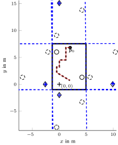
(a)

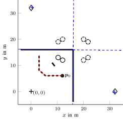
(b)

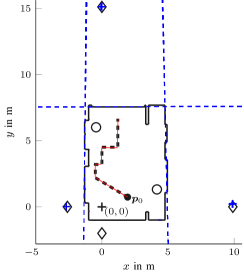
(c)

Figure 4: Scenarios used for numerical evaluation: (a) shows the scenario for Experiments $1$ and $2$ in Sections VI-C and VI-D. This scenario consists of a rectangular room with two PAs, i.e., there are four reflective surfaces. MVAs and VAs corresponding to single-bounce paths are shown. (b) shows the scenario for Experiment $3$ in Section VI-E which consists of two PAs, two reflective surfaces and an obstructing wall segment. MVAs and VAs corresponding to single-bounce paths are shown. (c) shows the scenario for Experiment 4 in Section VI-F. This scenario consists of a classroom with two PAs and four main reflective surfaces. Particle representations of the beliefs of MVA positions are shown as blue crosses. A line representing a reflecting surface is computed and shown as a dashed blue line for each particle. The geometric relations used to calculate a line from an MVA position have been presented in Section II.

VI Evaluation

The performance of the proposed MVA-based SLAM algorithm is validated and compared with the multipath-based SLAM algorithm from [3] that has been extended to use AOA measurements described here and in [4], the channel SLAM algorithm from [2], and the multipath assisted positioning algorithm from [40] using synthetic measurements as well as real RF measurements. Additional simulation results can be found in the supplementary material[37, Section LABEL:M-sec:app_results].

VI-A Common Setup and Performance Metrics

The agent’s state-transition pdf $f(\bm{x}_{n}|\bm{x}_{n-1})$, with $\bm{x}_{n}=[\bm{p}_{n}^{\text{T}}\;\bm{v}_{n}^{\text{T}}]^{\text{T}}$, is defined by a linear, near constant-velocity motion model [54, Sec. 6.3.2], i.e., $\bm{x}_{n}=\bm{A}\bm{x}_{n-1}+\bm{B}\bm{w}_{n}$. Here, $\bm{A}\in\mathbb{R}^{4\times 4}$ and $\bm{B}\in\mathbb{R}^{4\times 2}$ are as defined in [54, Sec. 6.3.2] (with sampling period $\Delta T=1\,\text{s}$), and the driving process $\bm{w}_{n}$ is iid across $n$, zero-mean, and Gaussian with covariance matrix $\sigma_{w}^{2}\mathbb{I}_{2}$, where $\mathbb{I}_{2}$ denotes the $2\times 2$ identity matrix and $\sigma_{w}$ denotes the acceleration noise standard deviation. For the sake of numerical stability, we introduced a small regularization noise to the PMVA state $\bm{p}_{s,\mathrm{mva}}$ at each time $n$, i.e., $\underline{\bm{p}}_{s,\mathrm{mva}}=\bm{p}_{s,\mathrm{mva}}+\bm{\omega}_{s}$, where $\bm{\omega}_{s}$ is iid across $s$, zero-mean, and Gaussian with covariance matrix $\sigma_{a}^{2}\mathbb{I}_{2}$. The particles for the initial agent state are drawn from a 4-D uniform distribution with center $\bm{x}_{0}=[\bm{p}_{0}^{\text{T}}\;0\;\,0]^{\text{T}}$, where $\bm{p}_{0}$ is the starting position of the actual agent trajectory, and the support of each position component about the respective center is given by $[-0.5\,\text{m},0.5\,\text{m}]$ and of each velocity component is given by $[-0.1\,\text{m/s},0.1\,\text{m/s}]$. At time $n=0$, the number of PMVAs is $S_{0}=0$, i.e., no prior map information is available. The prior distribution for new PMVA states $f_{\mathrm{n}}(\overline{\bm{y}}_{m,n})$ is uniform on the square region given by $[-15\,\text{m},\hskip 0.85358pt15\,\text{m}]\hskip 0.85358pt\times\hskip 0.85358pt[-15\,\text{m},\hskip 0.85358pt15\,\text{m}]$ around the center of the floor plan shown in Fig. 4a and the mean number of new PMVA is $\mu_{n}=0.05$. The probability of survival is $p_{\mathrm{s}}=0.999$, the confirmation and pruning thresholds are respectively ${p_{\mathrm{cf}}}=0.5$ and $p_{\mathrm{pr}}=10^{-3}$. We performed $500$ simulation runs. The performance of the different methods discussed is measured in terms of the root mean-square error (RMSE) of the agent position, as well as the optimal subpattern assignment (OSPA) error [55] of VAs and MVAs. Since the proposed method estimates MVAs, we first map MVA estimates to VA estimates following equation (3), before we compute OSPA errors of VAs. OSPA is a multi-object tracking metric that combines a localization error and a cardinality error into a single scalar score. As a result, it penalizes both state estimation inaccuracy and incorrect numbers of estimated features. We calculate the OSPA errors based on the Euclidean metric with cutoff parameter $c=5\,$m and order $p=1$. The mean OSPA (MOSPA) errors, RMSEs of each unknown variable are obtained by averaging over all converged simulation runs. We declare a simulation run to be converged if $\{\forall n:||\hat{\bm{x}}_{n}-\bm{x}_{n}||<5\,\text{m}\}$.

For synthetic measurements (Experiment $1$–$3$), we use the following common parameters. The detection probability of all paths is $\vspace{0.2mm}p_{\mathrm{d},ss,n}^{(j)}=p_{\mathrm{d},ss^{\prime},n}^{(j)}=p_{\mathrm{d}}=0.95$ for $(s,s)\in\mathcal{D}_{\text{S}}$ and $(s,s^{\prime})\in\tilde{\mathcal{D}}_{\text{D}}$, respectively. In addition, a mean number $\mu_{\mathrm{fp}}=1$ of false positive measurements $\bm{z}_{m,n}^{(j)}$ were generated according to the pdf $f_{\mathrm{fp}}(\bm{z}_{m,n}^{(j)})$ that is uniformly distributed on $[0\,\text{m},30\,\text{m}]$ for distance measurements and uniformly distributed on $[-\pi,\pi]$ for AOA measurements. In each simulation run, we generated noisy distance and AOA measurements according to (5) and (6) stacked into the vector $\bm{z}_{m,n}^{(j)}$.

VI-B Reference Methods

In the following sections, we compare the proposed MVA-based SLAM algorithm (PROP) to four different reference methods as described in the following:

1. MP-SLAM: The multipath-based SLAM algorithm from [3]. The method considered here is a combination of [3] and [4] since in [4] statistical model of [3] is extended to AOA measurements of MPCs. However, in contrast to [4], we do not use the component SNRs estimates of MPCs. Contrary to the method proposed in this paper, the reference method does rely on a much simpler statistical model without MVAs and ray-tracing. It thus cannot fuse data across propagation paths and VAs.

2. CH-SLAM: The channel SLAM algorithm from [2]. We only implemented the channel SLAM algorithm proposed in [2], not the full two-stage method that includes a channel estimator/tracker. Since the measurement-feature association is unknown, we perform Monte-Carlo data association for each particle separately, as it is commonly done in classical Rao-Blackwellized SLAM [56, Section 13], [10, 12].

3. MINT: The multipath-based positioning algorithm from [40], which assumes known map features (i.e., the VA positions are known).

4. LOS-MINT: A reduced version of MINT, where we only consider the PAs (i.e., no VAs).

We used $50000$ particles for PROP, MP-SLAM, MINT, and LOS-MINT. For CH-SLAM, we used $2000$ particles for the agent and $1000$ for the VAs. To analyze the performance gain due to exploiting double-bounce reflections, we generate two different datasets: (Setup-I) the full setup considering all VAs corresponding to single-bounce and double-bounce paths and (Setup-II) a reduced setup considering only VAs corresponding to single-bounce paths. If not stated differently, measurements are generated according to Setup-I.

VI-C Experiment 1: Comparison with Reference Methods

In this experiment, we compare PROP to MP-SLAM and CH-SLAM. Furthermore, we compare PROP with measurements generated without false positive measurements and missed detections termed ground-truth (GT) for Setup-I and Setup-II. We consider the indoor scenario shown in Figure 4a. We chose the scenario to be identical to [3] for easy comparison. The scenario consists of four reflective surfaces, i.e., $K=4$ MVAs and two PAs. The noise standard deviations for the LOS path are ${\sigma_{\mathrm{d}}}^{(j)}_{m,n}=0.05\,$m and ${\sigma_{\mathrm{\varphi}}}^{(j)}_{m,n}=10^{\circ}$, for single-bounce path are ${\sigma_{\mathrm{d}}}^{(j)}_{m,n}=0.10\,$m and ${\sigma_{\mathrm{\varphi}}}^{(j)}_{m,n}=15^{\circ}$, and for double-bounce path are ${\sigma_{\mathrm{d}}}^{(j)}_{m,n}=0.15\,$m and ${\sigma_{\mathrm{\varphi}}}^{(j)}_{m,n}=25^{\circ}$. The acceleration noise standard deviation is $\sigma_{w}=9\cdot 10^{-3}\,\text{m}/\text{s}^{2}$. As an example, Fig. 4a depicts for one simulation run the posterior PDFs represented by particles of the MVA positions and corresponding reflective surfaces as well as estimated agent tracks. Fig. 5a shows the MOSPA error for the two PAs and all associated VAs, Fig. 5b shows the MOSPA error for all MVAs, and Fig. 5c shows the RMSE of the agent’s position all versus time $n$. Fig. 5d shows the cumulative frequency of the agent errors (not excluding the diverged runs). Note that for all algorithms, none of the $500$ simulation runs diverged.

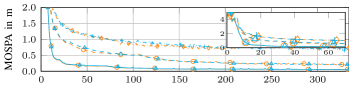
(a)

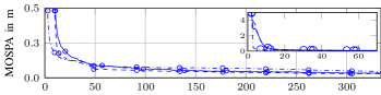
(b)

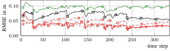
(c)

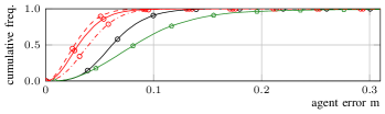
(d)

Figure 5: Performance results for Experiment 1 in Section VI-C: (a) MOSPA errors of the VAs of each PA, (b) MOSPA errors versus time of the MVAs, (c) RMSEs of the agent position versus time, (d) RMSEs versus time of the agent orientation, and (e) cumulative frequency of the RMSEs of the agent position.

The MOSPA error of PROP related to VAs and PAs is shown in Fig. 5a. It can be seen that the MOSPA drops significantly after only a few time steps. In contrast, MP-SLAM only converges rather slowly to a small mapping error. Furthermore, the MOSPA error of PROP converges along the agent track to a smaller value, i.e., to a smaller mapping error. This shows that PROP efficiently exploits all measurements for the map features provided by the PAs. Fig. 5b shows the MOSPA error of the MVA positions, which confirms the results seen in Fig. 5a. The RMSE of the agent position in 5c of PROP is considerably smaller than that of MP-SLAM along the whole agent track. Moreover, the RMSE of the agent position of PROP consistently decreases over time $n$, while that of MP-SLAM increases slightly during changes in the agent’s direction. PROP consistently demonstrates a statistically significant improvement in accuracy across all metrics, as illustrated in Figure 5d, facilitating the statistical dependencies across multiple paths and PAs. Furthermore, the results comparing Setup I and II using GT measurements illustrate that leveraging double-bounce paths systematically improves the performance of PROP. The average runtimes per time step for MATLAB implementations on a single core of Intel i7 CPUs (computer cluster with different versions of CPUs) were measured $4\,$s for PROP, $1.2\,$s for MP-SLAM, and $11\,$s for CH-SLAM.

VI-D Experiment 2: Varying Measurement Uncertainties

In this experiment, we analyze the performance of PROP with varying measurement noise standard deviations and compare it to MP-SLAM. In particular, we introduce factors $f_{\text{std, all}}$ and $f_{\text{std,los}}$. Both factors equally increase the base values of all measurement standard deviations in distance ${\sigma_{\mathrm{d}}}^{(j)}_{m,n}$ and AOA ${\sigma_{\mathrm{\varphi}}}^{(j)}_{m,n}$ for all $m\in M_{n}^{(j)}\,|\,j\in J,\,n\in\{1,\,...\,,N\}$ in a multiplicative way. Base values are set as the measurement standard deviations of Experiment 1. While $f_{\text{std,all}}$ affects measurements corresponding to PAs and MVAs, $f_{\text{std,los}}$ affects only measurement standard deviations corresponding to PAs (i.e., LOS measurements). The scenario is identical to experiment 1 of Section VI-C. Note that for all algorithms none of the $500$ simulation runs diverged.

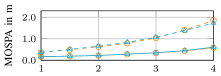
(a)

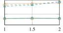
(b)

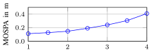
(c)

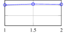
(d)

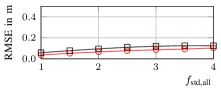
(e)

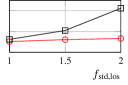
(f)

Figure 6: Performance results for Experiment 2 in Section VI-D for different noise standard deviations. Errors are averaged across time steps. Different noise standard deviations are used for all VAs and PAs: (a) MOSPA errors of VAs of each PA, (c) MOSPA errors of MVAs, and (e) RMSEs of the agent positions. Different noise standard deviations are used for all PAs: (b) MOSPA errors of VAs of each PA, (d) MOSPA errors of MVAs, and (f) RMSEs of the agent position.

Fig. 6a to 6f show the mean MOSPA of VAs and PAs, the mean MOSPA of MVAs or the mean agent RMSE, respectively, over all time steps $n$ as a function of $f_{\text{std,all}}$ or $f_{\text{std,los}}$. In particular, in Fig. 6a, 6c and 6e we varied $f_{\text{std,all}}$ and kept $f_{\text{std,los}}\triangleq 1$ fixed, while in Fig. 6b, 6d and 6f we varied $f_{\text{std,los}}$ and kept $f_{\text{std,all}}\triangleq 4$ fixed. The VAs MOSPA errors in Figs. 6a to 6d emphasize the observations of Experiment 1 (Section VI-C). All error values increase with increasing $f_{\text{std,all}}$. However, the MOSPA errors of the proposed method increases much slower. This is because the proposed method can fuse information provided by different PAs and different propagation paths. In contrast, the agent RMSE in Fig. 6e remains constant for both methods as there is still enough information available for proper localization, mainly provided by the PAs. Thus, when additionally increasing $f_{\text{std,los}}$ in Fig. 6f, the RMSE of MP-SLAM significantly increases. In contrast, the agent RMSE of PROP remains approximately constant due to the increased map stability.

VI-E Experiment 3: Low Information and Obstructed LOS

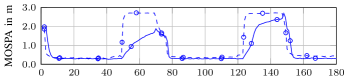
(a)

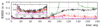
(b)

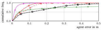
(c)

Figure 7: Performance results for Experiment 3 in Section VI-E: (a) MOSPA errors versus time of MVAs, (b) RMSEs versus time of the agent position, (c) RMSEs versus time of the agent orientation, (d) cumulative frequency of the RMSEs of the agent position (with outliers).

In this experiment, we analyze the performance of PROP in the scenario shown in Figure 4b. It contains only two reflective walls ($K=2$) while one short wall obstructs the LOS path, i.e., the path between PAs and the agent as well as the paths between VAs and agent[57]. The obstructing wall does not cause any VAs due to the geometric constellation. We compare MP-SLAM, MINT, and LOS-MINT. The scenario contains two PAs. We generate the distance and the AOA of the individual MPC parameters according to a RF signal model [24]. We assume the agent has a $3\times 3$ uniform rectangular array ($H=9$) with an inter-element spacing of $2$ cm. The transmit signal spectrum has a root-raised-cosine shape, with a roll-off factor of $0.6$ and a $3$-dB bandwidth of $B=500\,\mathrm{MHz}$ centered at $6\,\mathrm{GHz}$ resulting in a sampling time of $T_{\text{s}}=1/(1.6\,B)$. The amplitude of each MPC is assumed to follow free-space path loss and is attenuated by $3$ dB after each reflection. The SNR output at $1$ m distance to the agent is assumed to be $38$ dB. The measurement noise standard deviations are calculated based on the Fisher information [7, 4, 24]. The acceleration noise standard deviation is $\sigma_{w}=0.02\,\text{m}/\text{s}^{2}$.

Fig. 7a shows the MOSPA error for all MVAs, Fig. 7b shows the RMSE of the agent’s position for converged simulation runs, all versus time $n$. Finally, Fig. 7c shows the cumulative frequency of all agent’s position errors (not excluding the diverged runs). We show results for all investigated algorithms, where solid lines correspond to Setup-I and dashed lines correspond to Setup-II as described above. For PROP and MP-SLAM, none of the $500$ simulation runs diverged, but $30\,$% of the simulation runs diverged for LOS-MINT. LOS-MINT performs poorly, as in the central part of the track ($n=93$ to $n=107$), the LOS to all anchors is obstructed. This leads to LOS-MINT tending to choose an MPC as the LOS hypothesis as the agent state gradually becomes more uncertain. Figure 7b illustrates the benefits of PROP with respect to MP-SLAM, as it systematically leverages both PAs as well as both single-bounce and double-bounce propagation paths to infer the map features leading to a reduction in the RMSE of the agent’s position. Furthermore, Figure 7c statistically shows that this fusion results in fewer instances of large agent errors and that PROP consistent outperforms MP-SLAM. A possible explanation is the increased presence of MVAs and their corresponding reflective surfaces, which are more likely to exist due to the additional double-bounce measurement update.Although the single-bounce paths may not be visible, their absence is compensated by the fact that the proposed method performs data fusion across multiple propagation paths, as observed in Figure 7a. In contrast, MP-SLAM independently estimates each VA, thus lacking this advantageous feature. MINT has perfect (prior) knowledge of the VA positions and, thus, provides a lower bound for VA-based SLAM algorithms. PROP, which exploits double-bounce propagation paths, comes close to approaching this lower bound. Note that, in Figure 7b, between $n=0$ and $n=80$, LOS-MINT shows a slightly higher positioning accuracy compared to the proposed method. This difference is due to the uncertainty in MVA positions. A theoretical analysis on how uncertainty of map information affects the positioning accuracy of the agent is provided in [8, 9].

VI-F Experiment 4: Validation Using Measured Radio Signals

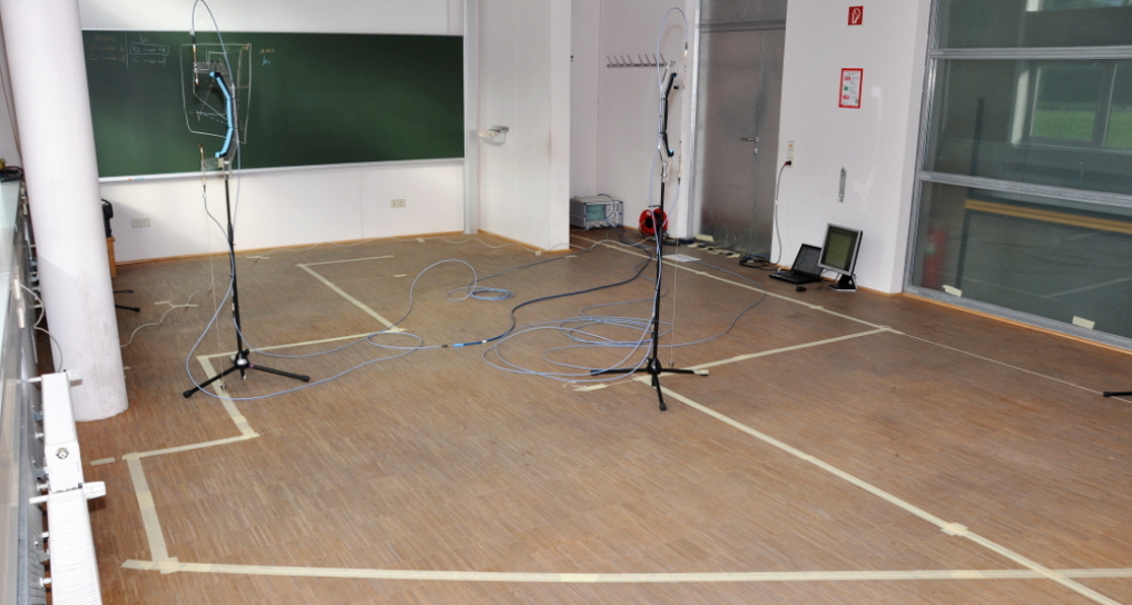
Figure 8: Picture of the classroom used for data collection.

To validate the applicability of the proposed MVA-based SLAM algorithm to real RF measurements, we use data collected in a classroom shown in Fig. 8 at TU Graz, Austria. More details about the measurement environment and VA calculations can be found in [58, 3, 6]. On the PA side, a dipole-like antenna with an approximately uniform radiation pattern in the azimuth plane and zeros in the floor and ceiling directions was used. At each agent position, the same antenna was deployed multiple times on a $3\times 3$, 2-D grid to yield a virtual uniform rectangular array with an inter-element spacing of $2$ cm. The UWB signals are measured at $180$ agent positions along a trajectory with position spacing of approx. $5$ cm as shown in Fig. 4c using an M-sequence correlative channel sounder with frequency range $3.1\textendash 10.6\,$GHz. Within the measured frequency-band, the actual signal spectrum was selected by a filter with root-raised-cosine shape, with a roll-off factor of $0.6$ and a $3$-dB bandwidth of $B=1\,\mathrm{GHz}$ centered at $6\,\mathrm{GHz}$. The received signal is critically sampled with $T_{\text{s}}=1/(1.6\,B)$ and artificial AWGN is added such that the output signal-to-noise-ratio is $\acs{snr}=30$ dB. We apply a variational sparse Bayesian parametric channel estimation algorithm [18] to acquire the $M_{n}^{(j)}$ distance estimates ${z_{\text{d}}}_{m,n}^{(j)}$ and AOA estimates ${z_{\varphi}}_{m,n}^{(j)}$ of MPCs. The corresponding noise standard deviations are calculated based on the Fisher information [7, 4, 24]. Compared to the synthetic setup, we changed the mean number of false alarm measurements to $\mu_{\mathrm{fp}}=3$, the detection probability to $p_{\text{d}}=0.7$, regularization noise standard deviation to $\sigma_{a}=2\cdot 10^{-3}\,\text{m}$, and the acceleration noise standard deviation to $\sigma_{w}=0.0114\,\text{m}/\text{s}^{2}$. Note that for all algorithms, none of the $500$ simulation runs diverged.

Fig. 4c depicts for one simulation run the posterior PDFs represented by particles of the MVA positions and corresponding reflective surfaces as well as estimated agent tracks. PROP can identify the main reflective surfaces of the room (The lower wall is only visible at the beginning of the agent track since the reflection coefficient is very low). Although the walls have a rich geometric structure (windows, doors, etc.) and generate many MPCs estimates, i.e., measurements, PROP robustly estimates the main walls. Fig. 9 compares PROP and MP-SLAM in terms of the agent RMSE. Fig. 9a shows the RMSE of the agent’s position, and Fig. 9b shows the RMSE of the agent’s orientation for simulation runs, all versus time $n$. The comparison of the position RMSEs shows a similar behavior as for synthetic measurements (see Fig. 5), i.e., PROP outperforms MP-SLAM. The mapping capability and low agent RMSEs of PROP, when applied to real RF signals, demonstrate the high potential of PROP for accurate and robust RF-based localization.

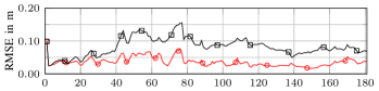
(a)

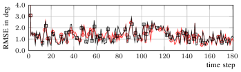
(b)

Figure 9: Performance results for Experiment 4 in Sec VI-F: (a) RMSEs versus time of the agent position and (b) RMSEs versus time of the agent orientation.

VII Conclusions

In this paper, we introduced data fusion for multipath-based SLAM. A key novelty of our approach is to represent each reflective surface in the propagation environment by a single MVA. In this way, we address a key limitation of existing multipath-based SLAM methods, which represent every propagation path by a VA and thus neglect inherent geometrical constraints across different paths that interact with the same reflective surface. As a result, the accuracy and speed of existing multipath-based SLAM methods are limited. A key aspect in leveraging the advantages of the introduced MVA-based model was to check the availability of single-bounce and double-bounce propagation paths at potential agent positions by means of ray-tracing (RT). Availability checks were directly integrated into the statistical model as detection probabilities of paths. Our numerical simulation results demonstrated significant improvements in estimation accuracy and mapping speed compared to state-of-the-art multipath-based SLAM methods. Looking forward, we expect to extend our approach to large-scale scenarios and more realistic 3-D environments. We expect such an extension to yield significantly increased computational complexity due to an increased dimensionality of the states to be estimated and an increased number of MVAs due to floor and ceiling surfaces. Promising directions for future research also include an extension to multiple-measurement-to-feature data association [25, 59] and an advanced MVA model, where the length and shape of reflective surfaces [16] are also taken into account. Another future research venue aims at incorporating amplitude information to make detection probabilities and measurement variances adaptive [4, 24, 57].

Erik Leitinger (Member, IEEE) received his MSc and PhD degrees (with highest honors) in electrical engineering from Graz University of Technology, Austria in 2012 and 2016, respectively. He was postdoctoral researcher at the department of Electrical and Information Technology at Lund University from 2016 to 2018. He is currently a University Assistant at Graz University of Technology. Dr. Leitinger served as co-chair of the special session ”Synergistic Radar Signal Processing and Tracking” at the IEEE Radar Conference in 2021. He is co-organizer of the special issue ”Graph-Based Localization and Tracking” in the Journal of Advances in Information Fusion (JAIF). Dr. Leitinger received an Award of Excellence from the Federal Ministry of Science, Research and Economy (BMWFW) for his PhD Thesis. He is an Erwin Schrödinger Fellow. His research interests include inference on graphs, localization and navigation, machine learning, multiagent systems, stochastic modeling and estimation of radio channels, and estimation/detection theory.

Alexander Venus (Student Member, IEEE) received his BSc and MSc degrees (with highest honors) in biomedical engineering and information and communication engineering from Graz University of Technology, Austria in 2012 and 2015, respectively. He was a research and development engineer at Anton Paar GmbH, Graz from 2014 to 2019. He is currently a project assistant at Graz University of Technology, where he is pursuing his Ph.D. degree. His research interests include radio-based localization and navigation, statistical signal processing, estimation/detection theory, machine learning and error bounds.

Bryan Teague (Member, IEEE) is a technical staff member at MIT Lincoln Laboratory. He received an MS degree in aerospace engineering from the Massachusetts Institute of Technology (MIT), Cambridge, Massachusetts, in 2017, and a BS (with highest honors) degree in engineering from Harvey Mudd College, Claremont, California, in 2010. He was a member of Wireless Information and Network Sciences Laboratory, Massachusetts Institute of Technology (MIT) from 2015 to 2017. He is a winner of a 2018 R&D100 innovation award. His research interests include probabilistic inference, optimal control, radio frequency technologies, and decentralized intelligence.

Florian Meyer (Member, IEEE) received the MSc and PhD degrees (with highest honors) in electrical engineering from TU Wien, Vienna, Austria in 2011 and 2015, respectively. He is an Assistant Professor with the University of California San Diego, La Jolla, CA, jointly between the Scripps Institution of Oceanography and the Electrical and Computer Engineering Department. From 2017 to 2019 he was a Postdoctoral Fellow and Associate with the Laboratory for Information & Decision Systems at the Massachusetts Institute of Technology, Cambridge, MA, and from 2016 to 2017 he was a Research Scientist with the NATO Centre for Maritime Research and Experimentation, La Spezia, Italy. Prof. Meyer is the recipient of the 2021 ISIF Young Investigator Award, a 2022 NSF CAREER Award, a 2022 DARPA Young Faculty Award, and a 2023 ONR Young Investigator Award. He is an Associate Editor with the IEEE Transactions on Aerospace and Electronic Systems and the ISIF Journal of Advances in Information Fusion and was a keynote speaker at the IEEE Aerospace Conference in 2020. His research interests include statistical signal processing, high-dimensional and nonlinear estimation, inference on graphs, machine perception, and graph neural networks.

References

- [1] K. Witrisal, P. Meissner, E. Leitinger, Y. Shen, C. Gustafson, F. Tufvesson, K. Haneda, D. Dardari, A. F. Molisch, A. Conti, and M. Z. Win, “High-accuracy localization for assisted living: 5G systems will turn multipath channels from foe to friend,” IEEE Signal Process. Mag., vol. 33, no. 2, pp. 59–70, Mar. 2016.
- [2] C. Gentner, T. Jost, W. Wang, S. Zhang, A. Dammann, and U. C. Fiebig, “Multipath assisted positioning with simultaneous localization and mapping,” IEEE Trans. Wireless Commun., vol. 15, no. 9, pp. 6104–6117, Sept. 2016.
- [3] E. Leitinger, F. Meyer, F. Hlawatsch, K. Witrisal, F. Tufvesson, and M. Z. Win, “A belief propagation algorithm for multipath-based SLAM,” IEEE Trans. Wireless Commun., vol. 18, no. 12, pp. 5613–5629, Dec. 2019.
- [4] E. Leitinger, S. Grebien, and K. Witrisal, “Multipath-based SLAM exploiting AoA and amplitude information,” in Proc. IEEE ICCW-19, Shanghai, China, May 2019, pp. 1–7.
- [5] R. Mendrzik, F. Meyer, G. Bauch, and M. Z. Win, “Enabling situational awareness in millimeter wave massive MIMO systems,” IEEE J. Sel. Topics Signal Process., vol. 13, no. 5, pp. 1196–1211, Sep. 2019.
- [6] E. Leitinger, P. Meissner, C. Rudisser, G. Dumphart, and K. Witrisal, “Evaluation of position-related information in multipath components for indoor positioning,” IEEE J. Sel. Areas Commun., vol. 33, no. 11, pp. 2313–2328, Nov. 2015.
- [7] T. Wilding, S. Grebien, E. Leitinger, U. Mühlmann, and K. Witrisal, “Single-anchor, multipath-assisted indoor positioning with aliased antenna arrays,” in Proc. Asilomar-18, Pacifc Grove, CA, USA, Oct. 2018.
- [8] A. Shahmansoori, G. E. Garcia, G. Destino, G. Seco-Granados, and H. Wymeersch, “Position and orientation estimation through millimeter-wave MIMO in 5G systems,” IEEE Trans. Wireless Commun., vol. 17, no. 3, pp. 1822–1835, Mar. 2018.
- [9] R. Mendrzik, H. Wymeersch, G. Bauch, and Z. Abu-Shaban, “Harnessing NLOS components for position and orientation estimation in 5G millimeter wave MIMO,” IEEE Trans. Wireless Commun., vol. 18, no. 1, pp. 93–107, Jan. 2019.
- [10] H. Durrant-Whyte and T. Bailey, “Simultaneous localization and mapping: Part I,” IEEE Robot. Autom. Mag., vol. 13, no. 2, pp. 99–110, Jun. 2006.
- [11] M. Dissanayake, P. Newman, S. Clark, H. Durrant-Whyte, and M. Csorba, “A solution to the simultaneous localization and map building problem,” IEEE Trans. Robot. Autom., vol. 17, no. 3, pp. 229–241, Jun. 2001.
- [12] M. Montemerlo, S. Thrun, D. Koller, and B. Wegbreit, “FastSLAM: A factored solution to the simultaneous localization and mapping problem,” in Proc. AAAI-02, Edmonton, Canda, Jul. 2002, pp. 593–598.
- [13] J. Mullane, B.-N. Vo, M. Adams, and B.-T. Vo, “A random-finite-set approach to Bayesian SLAM,” IEEE Trans. Robot., vol. 27, no. 2, pp. 268–282, Apr. 2011.
- [14] H. Deusch, S. Reuter, and K. Dietmayer, “The labeled multi-Bernoulli SLAM filter,” IEEE Signal Process. Lett., vol. 22, no. 10, pp. 1561–1565, Oct. 2015.
- [15] C. Cadena, L. Carlone, H. Carrillo, Y. Latif, D. Scaramuzza, J. Neira, I. Reid, and J. J. Leonard, “Past, present, and future of simultaneous localization and mapping: Toward the robust-perception age,” IEEE Trans. Robot., vol. 32, no. 6, pp. 1309–1332, Dec 2016.
- [16] X. Chu, Z. Lu, D. Gesbert, L. Wang, X. Wen, M. Wu, and M. Li, “Joint vehicular localization and reflective mapping based on team channel-SLAM,” IEEE Trans. Wireless Commun., pp. 1–1, Apr. 2022.
- [17] J. Yang, C.-K. Wen, S. Jin, and X. Li, “Enabling plug-and-play and crowdsourcing SLAM in wireless communication systems,” IEEE Trans. Wireless Commun., vol. 21, no. 3, pp. 1453–1468, Aug. 2022.
- [18] D. Shutin, W. Wang, and T. Jost, “Incremental sparse Bayesian learning for parameter estimation of superimposed signals,” in Proc. SAMPTA-2013, no. 1, Sept. 2013, pp. 6–9.
- [19] M. A. Badiu, T. L. Hansen, and B. H. Fleury, “Variational Bayesian inference of line spectra,” IEEE Trans. Signal Process., vol. 65, no. 9, pp. 2247–2261, May 2017.
- [20] T. L. Hansen, B. H. Fleury, and B. D. Rao, “Superfast line spectral estimation,” IEEE Trans. Signal Process., vol. PP, no. 99, pp. 2511 – 2526, Feb. 2018.
- [21] S. Grebien, E. Leitinger, B. H. Fleury, and K. Witrisal, “Super-resolution channel estimation including the dense multipath component — A sparse variational Bayesian approach,” ArXiv e-prints, 2023. [Online]. Available: https://arxiv.org/abs/2308.01702
- [22] A. Richter, “Estimation of Radio Channel Parameters: Models and Algorithms,” Ph.D. dissertation, TU Ilmenau, 2005.
- [23] J. Salmi, A. Richter, and V. Koivunen, “Detection and tracking of MIMO propagation path parameters using state-space approach,” IEEE Trans. Signal Process., vol. 57, no. 4, pp. 1538–1550, Apr. 2009.
- [24] X. Li, E. Leitinger, A. Venus, and F. Tufvesson, “Sequential detection and estimation of multipath channel parameters using belief propagation,” IEEE Trans. Wireless Commun., pp. 1–1, Apr. 2022.
- [25] F. Meyer and J. L. Williams, “Scalable detection and tracking of geometric extended objects,” IEEE Trans. Signal Process., vol. 69, pp. 6283–6298, Oct. 2021.
- [26] E. Leitinger, P. Meissner, M. Lafer, and K. Witrisal, “Simultaneous localization and mapping using multipath channel information,” in Proc. IEEE ICCW-15, London, UK, Jun. 2015, pp. 754–760.
- [27] M. Zhu, J. Vieira, Y. Kuang, K. Åström, A. F. Molisch, and F. Tufvesson, “Tracking and positioning using phase information from estimated multi-path components,” in Proc. IEEE ICCW-15, London, UK, Jun. 2015.
- [28] H. Kim, K. Granström, L. Svensson, S. Kim, and H. Wymeersch, “PMBM-based SLAM filters in 5G mmWave vehicular networks,” IEEE Trans. Veh. Technol., pp. 1–1, May 2022.
- [29] H. Kim, K. Granström, L. Gao, G. Battistelli, S. Kim, and H. Wymeersch, “5G mmWave cooperative positioning and mapping using multi-model PHD filter and map fusion,” IEEE Trans. Wireless Commun., vol. 19, no. 6, pp. 3782–3795, Mar. 2020.
- [30] G. Steinböck, M. Gan, P. Meissner, E. Leitinger, K. Witrisal, T. Zemen, and T. Pedersen, “Hybrid model for reverberant indoor radio channels using rays and graphs,” IEEE Trans. Antennas Propag., vol. 64, no. 9, pp. 4036–4048, Sept. 2016.
- [31] S.-W. Ko, H. Chae, K. Han, S. Lee, D.-W. Seo, and K. Huang, “V2X-based vehicular positioning: Opportunities, challenges, and future directions,” IEEE Wireless Commun., vol. 28, no. 2, pp. 144–151, Mar. 2021.
- [32] P. Koivumäki, A. Karttunen, and K. Haneda, “Wave scatterer localization in outdoor-to-indoor channels at 4 and 14 GHz,” in Proc. IEEE EuCAP, May 2022, pp. 1–5.
- [33] Z. Li, F. Jiang, H. Wymeersch, and F. Wen, “An iterative 5G positioning and synchronization algorithm in NLOS environments with multi-bounce paths,” IEEE Wireless Commun. Lett., vol. 12, no. 5, pp. 804–808, Feb. 2023.
- [34] J. Borish, “Extension of the image model to arbitrary polyhedra,” JASA, vol. 75, no. 6, pp. 1827–1836, Mar. 1984.
- [35] J. McKown and R. Hamilton, “Ray tracing as a design tool for radio networks,” IEEE Netw., vol. 5, no. 6, pp. 27–30, Nov. 1991.
- [36] J. S. Lu, E. M. Vitucci, V. Degli-Esposti, F. Fuschini, M. Barbiroli, J. A. Blaha, and H. L. Bertoni, “A discrete environment-driven GPU-based ray launching algorithm,” IEEE Trans. Antennas Propag., vol. 67, no. 2, pp. 1180–1192, Nov. 2019.
- [37] E. Leitinger, A. Venus, B. Teague, and F. Meyer, “Data fusion for multipath-based SLAM: Combining information from multiple propagation paths,” ArXiv e-prints, 2022. [Online]. Available: https://arxiv.org/abs/2211.09241
- [38] E. Leitinger and F. Meyer, “Data fusion for multipath-based SLAM,” in Proc. Asilomar-20, Pacifc Grove, CA, USA, Oct. 2020, pp. 934–939.
- [39] E. Leitinger, B. Teague, W. Zhang, M. Liang, and F. Meyer, “Data fusion for radio frequency SLAM with robust sampling,” in Proc. Fusion-22, Linköping, Sweden, Jul. 2022, pp. 1–6.
- [40] E. Leitinger, F. Meyer, P. Meissner, K. Witrisal, and F. Hlawatsch, “Belief propagation based joint probabilistic data association for multipath-assisted indoor navigation and tracking,” in Proc. ICL-GNSS-16, Barcelona, Spain, June 2016, pp. 1–6.
- [41] B. Etzlinger, F. Meyer, F. Hlawatsch, A. Springer, and H. Wymeersch, “Cooperative simultaneous localization and synchronization in mobile agent networks,” IEEE Trans. Signal Process., vol. 65, no. 14, pp. 3587–3602, July 2017.
- [42] J. Kulmer, E. Leitinger, S. Grebien, and K. Witrisal, “Anchorless cooperative tracking using multipath channel information,” IEEE Trans. Wireless Commun., vol. 17, no. 4, pp. 2262–2275, Apr. 2018.
- [43] F. Meyer, P. Braca, P. Willett, and F. Hlawatsch, “A scalable algorithm for tracking an unknown number of targets using multiple sensors,” IEEE Trans. Signal Process., vol. 65, no. 13, pp. 3478–3493, July 2017.
- [44] F. Meyer, T. Kropfreiter, J. L. Williams, R. Lau, F. Hlawatsch, P. Braca, and M. Z. Win, “Message passing algorithms for scalable multitarget tracking,” Proc. IEEE, vol. 106, no. 2, pp. 221–259, Feb. 2018.
- [45] M. Bayati, D. Shah, and M. Sharma, “Max-product for maximum weight matching: Convergence, correctness, and LP duality,” IEEE Trans. Inf. Theory, vol. 54, no. 3, pp. 1241–1251, Mar. 2008.
- [46] M. Chertkov, L. Kroc, F. Krzakala, M. Vergassola, and L. Zdeborová, “Inference in particle tracking experiments by passing messages between images,” PNAS, vol. 107, no. 17, pp. 7663–7668, Apr. 2010.
- [47] J. Williams and R. Lau, “Approximate evaluation of marginal association probabilities with belief propagation,” IEEE Trans. Aerosp. Electron. Syst., vol. 50, no. 4, pp. 2942–2959, Oct. 2014.
- [48] F. Antonio, “Iv.6 - faster line segment intersection,” in Graphics Gems III. San Francisco: Morgan Kaufmann, 1992, pp. 199–202.
- [49] H. V. Poor, An Introduction to Signal Detection and Estimation, 2nd ed. New York: Springer-Verlag, 1994.
- [50] F. Kschischang, B. Frey, and H.-A. Loeliger, “Factor graphs and the sum-product algorithm,” IEEE Trans. Inf. Theory, vol. 47, no. 2, pp. 498–519, Feb. 2001.
- [51] F. Meyer, O. Hlinka, H. Wymeersch, E. Riegler, and F. Hlawatsch, “Distributed localization and tracking of mobile networks including noncooperative objects,” IEEE Trans. Signal Inf. Process. Netw., vol. 2, no. 1, pp. 57–71, Mar. 2016.
- [52] H.-A. Loeliger, “An introduction to factor graphs,” IEEE Signal Process. Mag., vol. 21, no. 1, pp. 28–41, Feb. 2004.
- [53] Y. Bar-Shalom, P. K. Willett, and X. Tian, Tracking and Data Fusion: A Handbook of Algorithms. Storrs, CT: Yaakov Bar-Shalom, 2011.
- [54] Y. Bar-Shalom, X. R. Li, and T. Kirubarajan, Estimation with Applications to Tracking and Navigation: Algorithms and Software for Information Extraction. Hoboken, NJ: John Wiley and Sons, July 2001.
- [55] D. Schuhmacher, B.-T. Vo, and B.-N. Vo, “A consistent metric for performance evaluation of multi-object filters,” IEEE Trans. Signal Process., vol. 56, no. 8, pp. 3447–3457, Aug. 2008.
- [56] S. Thrun, W. Burgard, and D. Fox, Probabilistic Robotics (Intelligent Robotics and Autonomous Agents). The MIT Press, 2005.
- [57] A. Venus, E. Leitinger, S. Tertinek, F. Meyer, and K. Witrisal, “Graph-based simultaneous localization and bias tracking for robust positioning in obstructed LOS situations,” in Proc. Asilomar-22, 2022, pp. 1–8.
- [58] P. Meissner, E. Leitinger, M. Lafer, and K. Witrisal, “MeasureMINT UWB database,” www.spsc.tugraz.at/tools/UWBmeasurements, 2013. [Online]. Available: www.spsc.tugraz.at/tools/UWBmeasurements
- [59] L. Wielandner, A. Venus, T. Wilding, and E. Leitinger, “Multipath-based SLAM for non-ideal reflective surfaces exploiting multiple-measurement data association,” ArXiv e-prints, vol. abs/2304.05680, 2023. [Online]. Available: http://arxiv.org/abs/2304.05680