Token Turing Machines

Abstract

We propose Token Turing Machines (TTM), a sequential, autoregressive Transformer model with memory for real-world sequential visual understanding. Our model is inspired by the seminal Neural Turing Machine, and has an external memory consisting of a set of tokens which summarise the previous history (i.e., frames). This memory is efficiently addressed, read and written using a Transformer as the processing unit/controller at each step. The model’s memory module ensures that a new observation will only be processed with the contents of the memory (and not the entire history), meaning that it can efficiently process long sequences with a bounded computational cost at each step. We show that TTM outperforms other alternatives, such as other Transformer models designed for long sequences and recurrent neural networks, on two real-world sequential visual understanding tasks: online temporal activity detection from videos and vision-based robot action policy learning.

Code is publicly available at: https://github.com/google-research/scenic/tree/main/scenic/projects/token_turing.

1 Introduction

Processing long, sequential visual inputs in a causal manner is a problem central to numerous applications in robotics and vision. For instance, human activity recognition models for monitoring patients and elders are required to make real-time inference on ongoing activities from streaming videos. As the observations grow continuously, these models require an efficient way of summarizing and maintaining information in their past image frames with limited compute. Similarly, robots learning their action policies from training videos, need to abstract history of past observations and leverage it when making its action decisions in real-time. This is even more important if the robot is required to learn complicated tasks with longer temporal horizons.

A traditional way of handling online observations of variable sequence lengths is to use recurrent neural networks (RNNs), which are sequential, auto-regressive models [35, 13, 22]. As Transformers [64] have become the de facto model architecture for a range of perception tasks, several works have proposed variants which can handle longer sequence lengths [19, 61, 67]. However, in streaming, or sequential inference problems, efficient attention operations for handling longer sequence lengths themselves are often not sufficient since we do not want to run our entire transformer model for each time step when a new observation (e.g., a new frame) is provided. This necessitates developing models with explicit memories, enabling a model to fuse relevant past history with current observation to make a prediction at current time step. Another desideratum for such models, to scale to long sequence lengths, is that the computational cost at each time step should be constant, regardless of the length of the previous history.

In this paper, we propose Token Turing Machines (TTMs), a sequential, auto-regressive model with external memory and constant computational time complexity at each step. Our model is inspired by Neural Turing Machines [30] (NTM), an influential paper that was among the first to propose an explicit memory and differentiable addressing mechanism. The original NTM was notorious for being a complex architecture that was difficult to train, and it has therefore been largely forgotten as other modelling advances have been made in the field. However, we show how we can formulate an external memory as well as a processing unit that reads and writes to this memory using Transformers (plus other operations which are common in modern Transformer architectures). Another key component of TTMs is a token summarization module, which provides an inductive bias that intuitively encourages the memory to specialise to different parts of its history during the reading and writing operations. Moreover, this design choice ensures that the computational cost of our network is constant irrespective of the sequence length, enabling scalable, real-time, online inference.

In contrast to the original NTM, our Transformer-based modernisation is simple to implement and train. We demonstrate its capabilities by achieving substantial improvements over strong baselines in two diverse and challenging tasks: (1) online temporal action detection (i.e., localisation) from videos and (2) vision-based robot action policy learning.

2 Related Work

Our TTM model is related to prior work on designing Transformers to process long sequence lengths and temporal context (e.g., videos), and also models to store and retrieve relevant information from internal/external memory.

Transformers for sequences.

Pairwise self-attention mechanism proposed in Transformer [64] has been very successful in many vision tasks, including the understanding of image sequences. Extending ViT [23], ViViT [3] and TimeSformer [4] represented video data, a series of space-time tokens. Transformers have since become state-of-the-art in video modeling, being able to handle multiple modalities like audio/text [49, 2] and scaling efficiently [24, 47].

One of the major challenges in using Transformers for sequential data is the well-known quadratic computation cost of self-attention. That is, as the number of frames in a video sequence increase, the computation grows quadratically which often soon becomes intractable. There is a wide body of work on reducing this to enable transformers to handle longer sequence lengths, as summarized in surveys such as [61, 60]. Common themes include local- or sparse-attention [71, 46, 11], pooling or reducing the number of tokens within the network [56, 37, 54] and approximations of the attention matrix [12, 65, 50].

However, in the sequential inference problems considered in this paper, efficient operations for handing longer sequence lengths are often not sufficient themselves, as we do not want to perform redundant operations at every new time step, when new input tokens are given.

Transformers with memories.

One manner of reducing redundancy over time-steps is to leverage models with memory. There are a number of works using Transformers to retrieve relevant information from external memories/knowledge bases [43, 5, 33, 67] or historical observations [7, 45, 54]. In comparison, the memory of our model is also based on historical observations of the model, which informs the current and future predictions; we learn to maintain/read/write to the memory. Another method for reusing computation from previous time steps is to perform causal attention. In this case, the previous activations of the model can be cached, as done in the original implementation of the Transformer [64]. However, with this approach, the computation cost at each step still linearly increases over time as the sequence length of previous tokens increase. Transformer-XL [19] builds upon this idea, and uses relative positional embeddings to make better use of previous history tokens. MemViT [66] also uses token activations from previous time-steps to increase the contextual information provided at the current time step. However, once again, the computational cost at each step still increases over time. [29, 21] introduced an approach to improve pairwise operations in Transformers by interacting with (external) shared workspace, which also could be viewed as memory read/write.

Sequential models.

The classical solution for dealing with long and variable sequence lengths are recurrent neural networks, which share the same parameters across multiple time-steps to be able to generalise to varying sequence lengths. LSTMs [35] and GRUs [13] are the most well-known form of these networks, as they were formulated to handle the “vanishing and exploding gradient” problem [34]. Video representations using them also have been common, traditionally [22]. Transformers have been adapted to recurrent networks as well, with models such as Block-Recurrent Transformers [36], which is an RNN with a transformer operating on a sequence (or block) of tokens, instead of traditional RNNs which have a single previouss state. [41] adds an external memory module to LSTMs/GRUs.

Neural Turing Machines.

Our model, however, is based on another formulation of RNNs, the Neural Turing Machine (NTM) [30]. This model architecture is based on the von Neumann computer architecture, and consists of a controller and external memory which is read and written to using explicit addressing operations in a differentiable manner. Its memory access mechanism was further extended in the subsequent work, DMC [31]. The original NTM was a complex model that was notorious for being difficult to train. Our formulation can be thought of as a modernisation of this architecture using Transformer-based operations as primitives. Our model is simple and easy to train, and we have also applied it to complex problems in computer vision (and visual robot learning) that the original NTM was never demonstrated for.

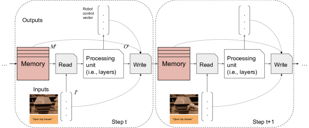
Figure 1: TTM overview with robot examples. Each dotted rectangle shows TTM at each step.

3 Token Turing Machines

Token Turing Machines are new sequential auto-regressive models, with core components being the (external) memory and the processing unit, as shown in Fig. 1. The memory at time step $t$, $M^{t}\in\mathbb{R}^{m\times d}$, consists of a set of $m$ tokens of dimensionality $d$. In Token Turing Machines (TTMs), the interface between the processing unit and memory are done purely in terms of “read” and “write” operations. The result of memory “read” is fed to the processing unit. The output from the processing unit is “written” to the memory.

As illustrated in Fig. 1, the input at time step $I^{t}\in\mathbb{R}^{n\times d}$, is merged with the memory $M^{t}$ to retrieve relevant tokens from both, which are then processed further to produce $O^{t}\in\mathbb{R}^{r\times d}$. The outputs of this step, along with the previous inputs and current memory are then used to write to the memory, $M^{t+1}$, which will be used at the next time step. As many sequential decision making tasks require predictions at each time step, we also include a linear output head at each step.

3.1 Memory Interface

There are several principles which motivate the design of our memory interface: Intuitively, we do not wish to read from (or write to) all memory tokens at each time step. This is because although the memory should contain (summarised) information from the entire past history, only some of this information may be relevant for the processing at the current stage. Therefore, we consider selective reading of a smaller subset of tokens to be a good inductive bias that will encourage the model to make use of a memory that stores relevant information over varying time scales Such “selective reading” is in contrast to most previous recurrent models (e.g., RNNs) directly digesting history vectors.

Moreover, there may be redundancies in the input stream, $I^{t}$, due to the information that we already have in our memory, $M^{t}$, and due to the data itself (for example, videos contain redundant frames; not all parts of an image are relevant to the task at hand). Therefore, a mechanism to summarise tokens, both from the memory and the input stream, is a core component of our approach. We discuss this summarisation procedure next in Sec. 3.1.1 before describing reading (Sec. 3.1.2), processing (Sec. 3.1.3) and writing (Sec. 3.1.4).

3.1.1 Token Summarisation

There are multiple methods of summarising a sequence of $p$ tokens with dimensionality $d$, $V\in\mathbb{R}^{p\times d}$, to $Z\in\mathbb{R}^{k\times d}$ where $k\ll p$. Examples include [56, 37, 70, 55, 25, 14] which have been proposed in the context of more efficient transformer backbones for processing higher-resolution images. We adopt a similar approach as a core component of our reading and writing mechanisms. Our method is based on [56, 37] motivated by the fact that these approaches are simple, fully-differentiable and have achieved strong results in a number of domains.

Concretely, we summarise a set of tokens $V$ by computing an importance weight vector, $w_{i}\in\mathbb{R}^{p}$ which we use to compute a weighted summation over the $p$ tokens. Note that we have $w_{i}$ for each output token, $i\in\{1,\ldots,k\}$, and it is computed with a learnable function taking the input $V$ itself, $\alpha_{i}(V)$. Here, such each importance weighting function is modeled either using a MLP or using a learned query vector, $q_{i}$, computed as:

$$w_{i} =\alpha_{i}(V)=\text{softmax}(\text{MLP}(V)),~{}~{}\text{or}$$ (1)

$$w_{i} =\alpha_{i}(V)=\text{softmax}(q_{i}V^{\top}/\sqrt{d}).$$ (2)

These weights are then used to perform a weighted summation of the inputs:

$$z_{i}=s_{i}(V)=w_{i}\cdot V=\alpha_{i}(V)\cdot V,$$ (3)

where each token $z_{i}$ summarises all the tokens from the complete set $V$, based on the dynamic weighting $w_{i}=\alpha_{i}(V)$. As we learn to summarize $p$ tokens into $k$ tokens, it computes a matrix $W=[w_{1},\cdots,w_{k}]$ of importance weights in practice.

Overall, we denote this summarisation function as $S_{k}:\mathbb{R}^{p\times d}\to\mathbb{R}^{k\times d}$, which we use for both memory read and write.

3.1.2 Reading from Memory

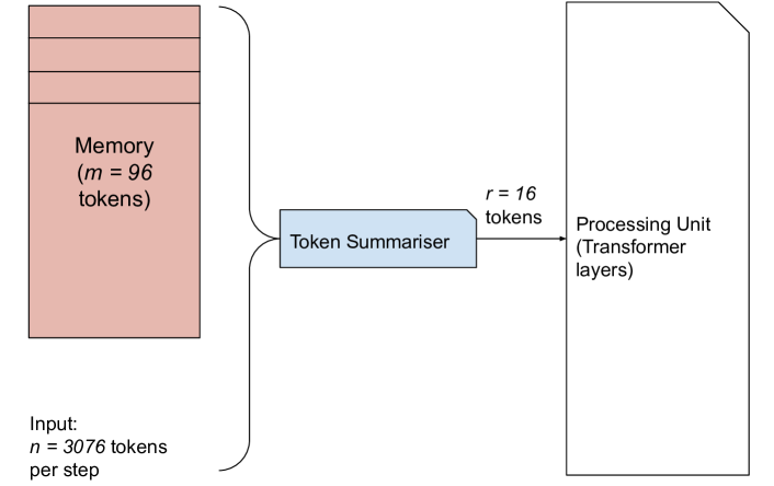
Figure 2: TTM Read. Note how it greatly reduces the computation of the subsequent processing module by summarising the input sequence as well.

In contrast to Neural Turing Machines [30], where inputs and memory are separately processed and merged later, we take a unified memory-input reading strategy. This is motivated by the fact that some of the inputs, $I^{t}$, are redundant given the information that we already have in memory.

As illustrated in Fig. 2, we concatenate the tokens in memory, $M^{t}$ composed of $m$ tokens, with the input stream, $I^{t}$ composed of $n$ tokens, and summarise these tokens into a smaller subset of $r$ tokens. Our read operator is thus defined as

$$Z^{t}=\text{Read}(M^{t},I^{t})=S_{r}([M^{t}||X^{t}]),$$ (4)

where $[M^{t}||X^{t}]$ denotes the concatenation of these two matrices. This essentially is a function of $\mathbb{R}^{(n+m)\times d}\to\mathbb{R}^{r\times d}$. Thus, the read operator filters the information in the memory and input which should be passed to the subsequent processing unit. Note that by reducing the number of tokens passed to the processing module, we also substantially reduce the computational cost of this stage.

Memory addressing by location using positional embedding

In principle, the token summarisation module described above enables content-based addressing of the memory. This was referred as “read by content” in the Neural Turing Machines. In order to also make the model take advantage of locations of the tokens within the memory (and also to distinguish tokens from memory vs. tokens from inputs), we add a learnable positional embedding [23] before each read module. This approach, fusing position information into the tokens, has an effect of read/write by location (+ content) without modifying the overall process.

3.1.3 Processing Unit

Our processing unit is a generic function, $O^{t}=\text{Process}(Z^{t})$, that operates on the $r$ tokens obtained from the read operation, $Z^{t}$. The processing function generates a set of $r$ output tokens, $O^{t}$, which are used in the subsequent write operation. Moreover, for tasks which require a prediction at each time-step, we add a linear output-head $Y^{t}=\text{Output}(O^{t})=W_{o}O^{t}$ to the output tokens.

In our experiments, we use a standard Transformer [64] and MLPMixer [62] as our processing unit, although other architectures are possible too.

3.1.4 Writing to Memory

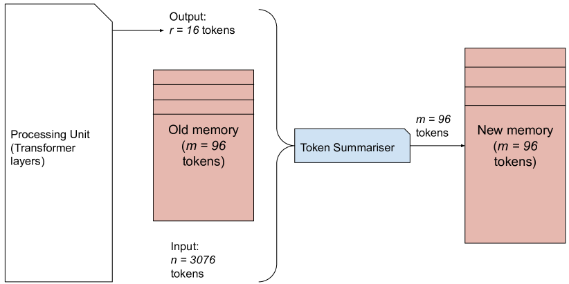
Figure 3: TTM Write, formulated as the token summarisation.

We also formulate our write operation as a token summarisation process, which we observed to be both simple and effective.

As illustrated in Fig. 3, our write mechanism preserves tokens in the memory, $M^{t}$, by learning to re-select them. And it adds new tokens to the memory by selecting them from either the output of the processing module, $O^{t}$, or from the inputs $I^{t}$. Therefore, we formulate our write operations as selecting $n$ tokens (i.e., the size of the memory) from the concatenation of current memory, input and output tokens, as denoted by

$$M^{t+1}=\text{Write}(M^{t},O^{t},I^{t})=S_{n}([M^{t}||O^{t}||I^{t}]).$$ (5)

Therefore, the tokens in memory will be erased if they are not re-selected. Similar to the read operation, positional embedding is used to distinguish tokens from memory, input, and output. This essentially is a function of $\mathbb{R}^{(n+m+r)\times d}\to\mathbb{R}^{m\times d}$.

3.2 Discussion

Our proposed Token Turing Machine can be viewed as a modernisation of Neural Turing Machines (NTM) [30] by using Transformer-based models for the processing unit and its interfaces with the (external) memory.

Our reading and writing mechanisms differ to NTM in that we use token summarisation (Sec. 3.1.1) as the core component that unifies the two operations. NTM, on the other hand, uses a complex range of “content” and “location” addressing strategies to produce the indices in the memory to read and write to, and learns a combination of matrix additions and deletions for the memory modifications.

And whilst we use a Transformer (or a Mixer) for the processing unit, NTM used either fully-connected feedforward or LSTM networks for its processing unit (or controller). The architectural choices of NTM meant that it was difficult to train in practice. On the other hand, we have not witnessed training instabilities with our TTM model in the experiments that we present next.

Both TTMs and NTMs in general could be viewed as a new form of recurrent neural networks. The operations in TTMs can be summarised, in the recurrent network form as:

$$Z^{t} =\text{Read}(I^{t},M^{t})$$ (6)

$$O^{t} =\text{Process}(Z^{t})$$ (7)

$$M^{t+1} =\text{Write}(M^{t},O^{t},I^{t})$$ (8)

$$Y^{t} =\text{Output}(O^{t})$$ (9)

where the functions Read(), Process(), Write(), and Output() are what we discussed in this section.

4 Experiments

4.1 Video Activity Detection

Activity Detection in videos focus on making fine-grained action predictions per every time step. In general, datasets for detection [8, 57, 69, 32], contain long-range videos with multiple overlapping activities, capturing an expressive temporal context. Hence, detection is more challenging compared to classification, which only makes a prediction once per video. Also, detection models often need to look at more frames to generate good representations in temporal context, which can be computationally expensive, particularly in Transformer-based architectures due to their quadratic cost.

We focus on making online inferences, generating activity predictions for each incoming frame. That is, the decision is made without accessing frames in future steps.

4.1.1 Dataset and Settings

Charades dataset [57] contains $\sim$9.8k videos of 157 daily household activities, separated into $\sim$7.9k training and $\sim$1.8k validation clips. Each video may include multiple overlapping activities (w/ an average of 6.8 activity instances per video), annotated with frame-level labels. The average length of a video is 30 seconds. This is a challenging setting, especially for temporal activity detection, as a model needs to predict multiple potential activity classes per each frame, considering the interactions between different activities and longer temporal context.

For our evaluation, we use the standard ‘charades_v1_localize’ setting, where we uniformly sample 25 frames from each video in the validation set and compute mean average precision (mAP).

We also use AVA v2.2 [32] as the secondary dataset to confirm the effectiveness of the TTM’s sequential modeling, specifically in spatio-temporal activity detection. AVA is a dataset composed of bounding box annotations of 80 atomic visual actions in 430 15-minute movie clips. We follow its standard setting, while using the Kinetics-400 for the backbone pretraining.

4.1.2 Baselines and Implementation

We use ViViT [3] as our backbone. As was done in its original work, we made ViViT represent 32 frame segments. Given a continuous sequence of frames, ViViT converts it into a sequence of representations where each element is from a 32-frame segment. We use ViViT-B with its original settings: the input frame resolution is 224-by-224, and the video patch size is $16\times 16\times 2$ (i.e., an image patch of $16\times 16$ over $2$ frames). It generates 14-by-14-by-16 (i.e., 3136) tokens, and this becomes our ‘step input’ for TTMs: $n=3136$. Alternatively, we do spatial average pooling per frame, getting 16 tokens per step: $n=16$

We tested various memory sizes ($m$), and we use $m=96$ as the default setting. The number of reads is $r=16$ (or $32$). The processing unit in TTMs is implemented to have a small overhead. In the case of using Transformers or MLPMixers, we used the hidden size of 512 and a total of four blocks. The training of the models was done by providing video segments of 6 steps (i.e., $32\times 6$ frames) at a time. We include the detailed training settings in Appendix.

Method	Setting	modality	mAP
I3D + super-events [52]	offline	RGB + Flow	19.41
I3D + super-events + TGM [53]	offline	RGB + Flow	22.30
I3D + STGCN [28]	offline	RGB + Flow	19.09
I3D + biGRU + VS-ST-MPNN [48]	offline	RGB + Object	23.7
Coarse-Fine (w/ X3D) [40]	offline	RGB	25.1
I3D + CTRN [16]	offline	RGB	25.3
I3D + MS-TCT [17]	offline	RGB	25.4
I3D + PDAN [18]	offline	RGB + Flow	26.5
I3D + CTRN [16]	offline	RGB + Flow	27.8
I3D [10]	online	RGB + Flow	17.22
X3D [26]	online	RGB	18.87
ViViT-B [3]	online	RGB	23.18
ViViT-B + TTM (ours)	online	RGB	26.34
ViViT-L [3]	online	RGB	26.01
ViViT-L + TTM (ours)	online	RGB	28.79

Table 1: Comparison with the state-of-the-art methods on Charades temporal activity detection.

4.1.3 Temporal Activity Detection Results

In Table 1, we compare TTMs with prior state-of-the-art in temporal activity detection on Charades. The previous work we compare against include multiple backbone architectures (e.g., I3D [10], X3D [26]) as well as different techniques for long-term temporal modeling on top of the backbones (e.g., super-events [52], TGM [53], Coarse-Fine [40, 39], and MS-TCT [17]).

Importantly, we grouped the approaches based on whether they support online inference or not. While most of the backbone models enable online inference by focusing on recent frames at hand, some approaches require a longer temporal window including future frames (e.g., the global snapshot of the entire video) to make a prediction for a given frame.

In addition, we compared TTMs with different sequential/temporal modeling architectures, applied on top of the same backbone model we use (i.e., ViViT). These include temporal Transformers and temporal MLPMixers [62], as well as more traditional sequential models like a LSTM. In addition, we implement a recurrent version of Transformers, which takes state tokens and input tokens to predict the next state tokens and output tokens. For temporal Transformers and MLPMixers, a temporal window of 6 steps is used. The models are over a fixed window, capturing $6\times 32=192$ frames. The raw output from ViViT has $14\times 14\times 16$ tokens per step, giving us a total of $3136\times 6=18816$ input tokens. We used aggressive (spatial) pooling and (temporal) striding to make their computational cost as low as TTMs, and FLOPS become comparable.

Table 2 shows the results. The FLOPS described are per-step inference time, excluding the backbone computation. We are able to confirm that TTM, due to its external memory interactions, enables much more efficient online inference compared to other types of sequential/temporal models. When TTM-Transformer and causal/recurrent Transformers are using the same number of input tokens (i.e., $n=16$), TTM spends around 1/2 FLOPS compared to the causal/recurrent Transformers (TTM 0.228 vs. causal/recurrent Transformers 0.523/0.410 GFLOPS), while TTM still outperforms them (TTM 26.24 vs. causal/recurrent Transformers 25.85/25.97 mAP). In addition, while other temporal models have difficulty scaling (i.e., with a large number of tokens) due to overfitting, TTM handles more tokens much more reliably.

Method	mAP	GFLOPS
ViViT only	23.18	-
Alternative temporal models
Temporal MLPMixer (tokens=96)	24.41	0.382
Causal Transformer (tokens=96)	25.85	0.523
Temporal Transformer (tokens=96)	25.61	1.269
Temporal MLPMixer (tokens=3360)	24.26	13.317
Causal Transformer (tokens=3360)	25.88	29.695
Temporal Transformer (tokens=3360)	25.53	112.836
Alternative recurrent networks
LSTM	23.96	0.107
Recurrent Transformer (tokens=16+16)	25.97	0.410
Recurrent Transformer (tokens=3136+16)	25.97	17.10
Token Turing Machines
TTM-Mixer ($n=16$)	25.83	0.089
TTM-Transformer ($n=16$)	26.24	0.228
TTM-Mixer ($n=3136$)	26.14	0.704
TTM-Transformer ($n=3136$)	26.34	0.842

Table 2: TTM vs. different sequence modeling methods. ViViT-B was used as the backbone. TTM-Transformer means we use Transformer as the processing unit, and TTM-Mixer means we use MLPMixer as the processing unit. FLOP measure is for computation in addition to the backbone.

4.1.4 Ablations

Here, we conduct a number of ablations to investigate different components of Token Turing Machines. We use ViViT-B as the backbone. Unless specified, the models use Transformer processing units by default, and MLP-based token summarisations. The number of input tokens per step is $n=3136$.

Processing units:

Table 4 compares TTMs with different processing units. The default processing unit, i.e., Transformer, is compared against MLPMixer and a simple MLP. We observe that MLPMixer-based TTM provides a good speed-accuracy trade-off.

Architecture	mAP	GFLOPS
MLP	23.34	0.689
MLPMixer	26.14	0.704
Transformer	26.34	0.842

Table 3: Using different processing unit architectures in TTMs.

Method	mAP	GFLOPS
Pooling	25.75	0.206
MLP	26.34	0.842
Latent query	26.75	8.537

Table 4: Different Token Summarisation

Token summarisation:

Table 4 compares different token summarisation methods used within TTMs. Essentially, we are comparing different form of the $\alpha_{i}$ function in Equation 1, which influences both memory read and write in TTMs. We compare the MLP-based $\alpha$, the latent query-based $\alpha$, and a simple pooling-based summarisation (i.e., no learning) method.

Method	mAP	GFLOPS
Concatenate (Memorizing Transformer-style)	20.97	0.920
Erase and Add (NTM-style write)	25.86	0.423
TTM without memory	22.65	0.842
TTM	26.34	0.842

Table 5: TTM vs. different history/memory update. They all use Transformer processing units, and MLP-based token summarisations. The number of input tokens per step, $n=3176$.

Different memory read/write:

We compare memory read/write mechanisms of TTMs with their alternatives, motivated by prior work including [30, 67]. Specifically, we implemented the memory write of concatenating every observed input tokens. We also implemented the memory write mechanism designed in [30]: write by erase and addition. Finally, a memory-free version of TTM was implemented to confirm the importance of the memory. This was done by zeroing out the memory of the TTM after each step, making it spend exactly the same amount of computation. Table 5 shows the results.

Model	mAP	+GFLOPS
MViT	26.2	-
+ memory (i.e., MeMViT [66])	28.5 (+2.3)	1.3
ViViT-B	25.2	-
+ TTM per video	27.9 (+2.7)	0.8
+ TTM per box (# layers=1)	31.3 (+6.1)	1.0
+ TTM per box (# layers=4)	31.5 (+6.3)	2.0

Table 6: Results on AVA 2.2, with the vanilla Kinetics-400 pretraining. We show FLOPS added by the sequential modeling per step. ViViT-B is the backbone for TTM, while MeMViT uses MViT.

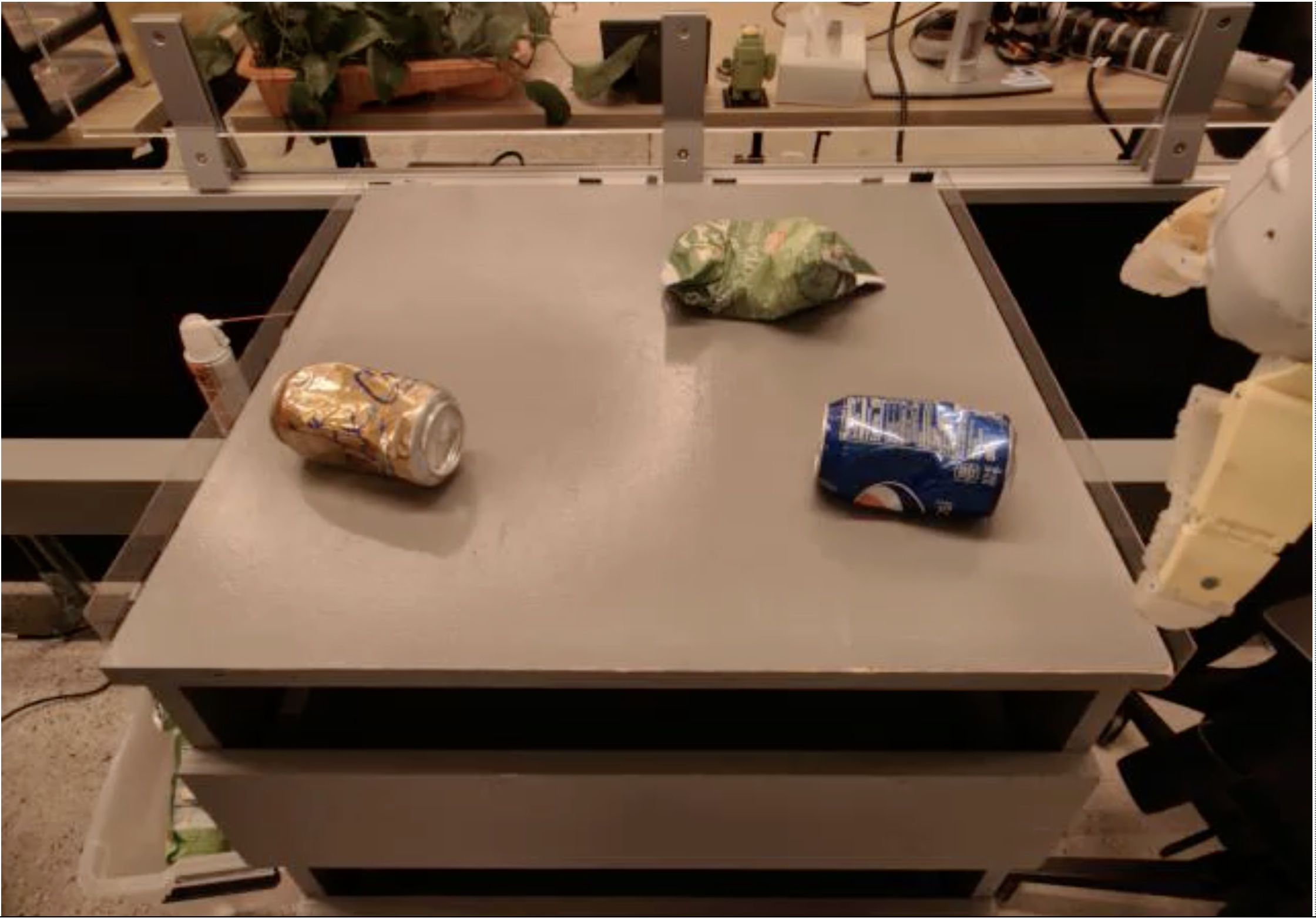
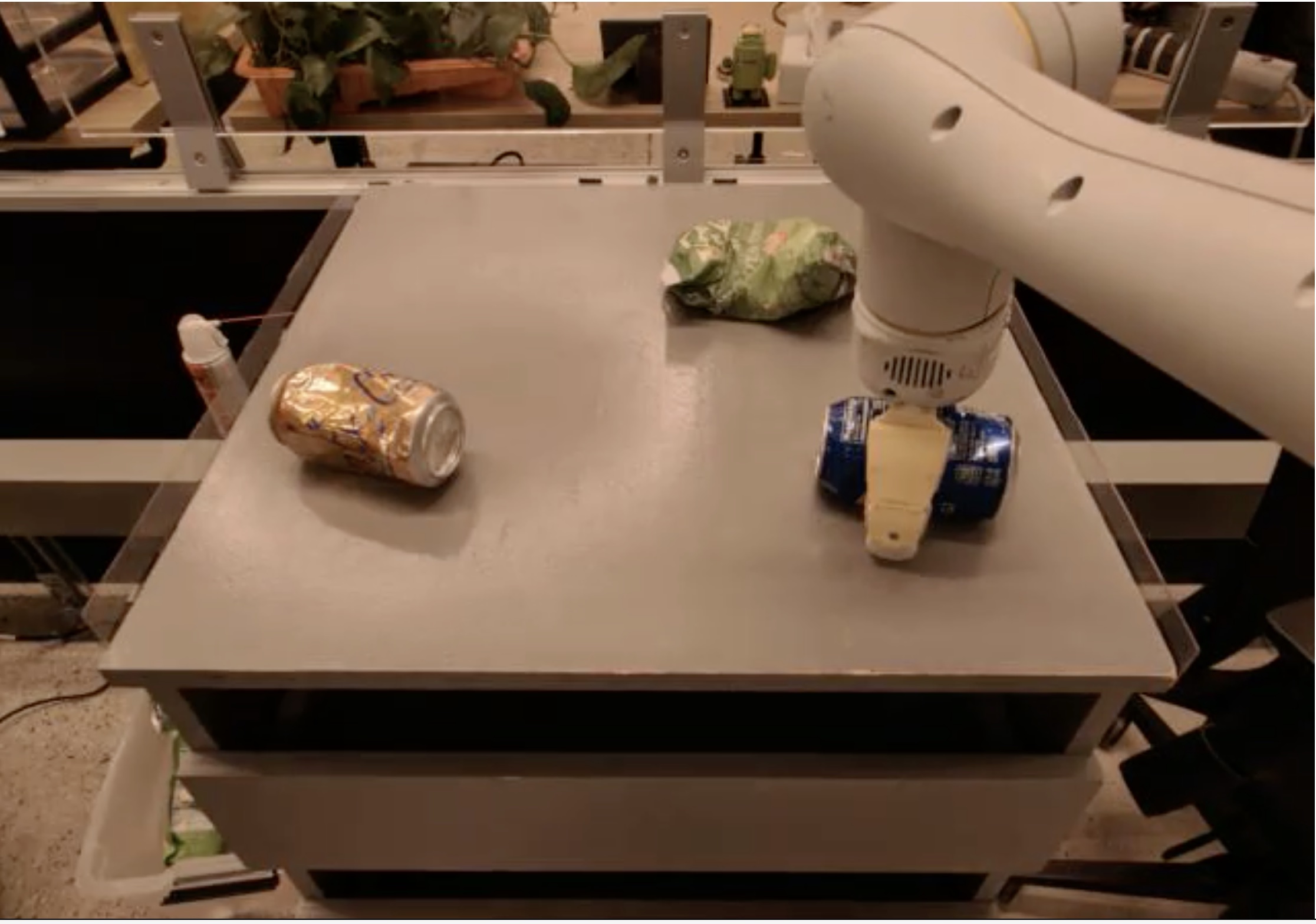
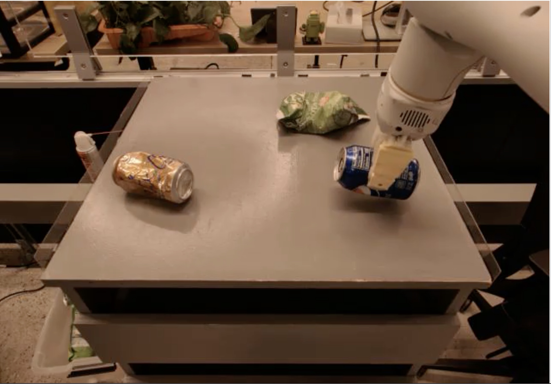
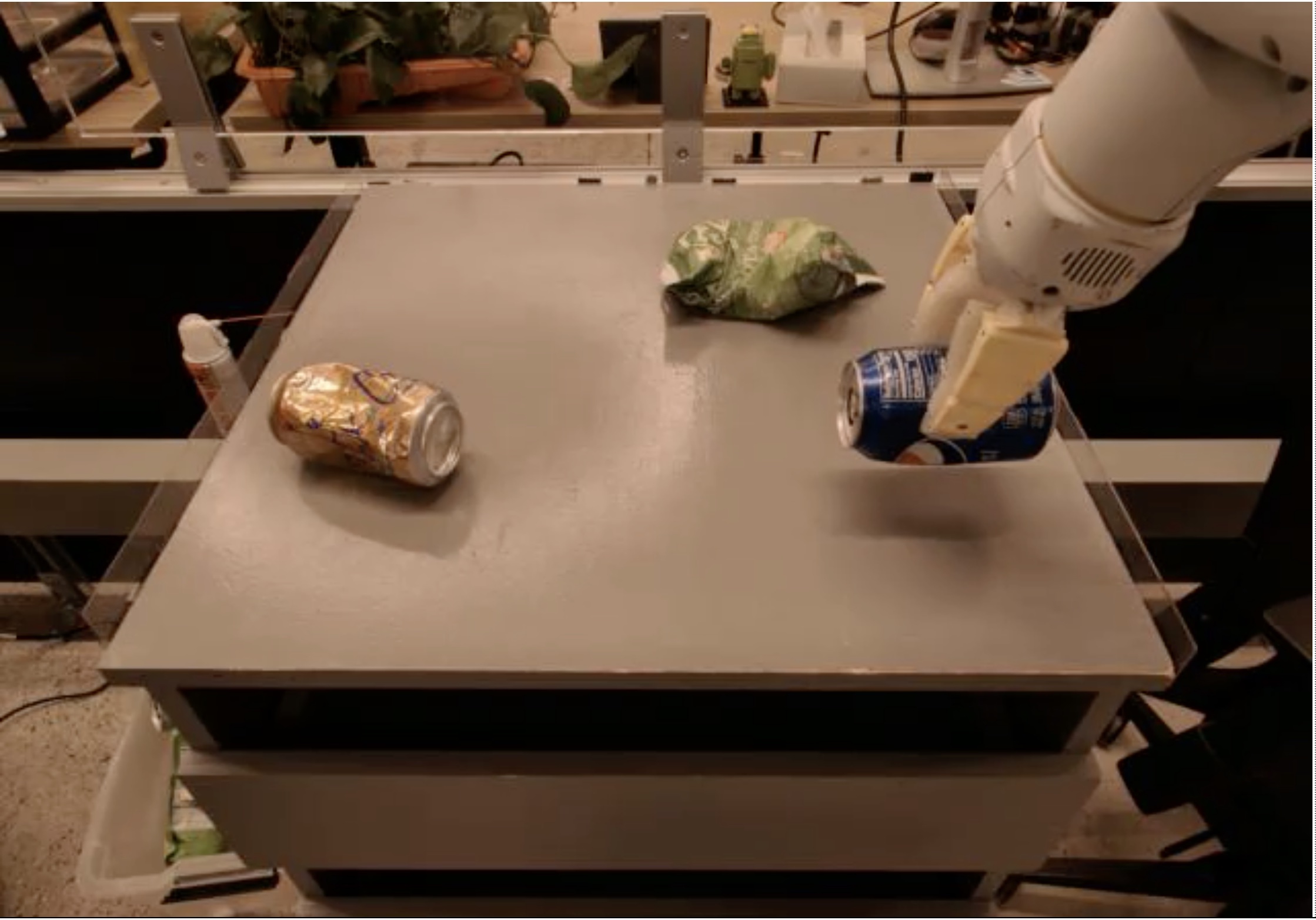
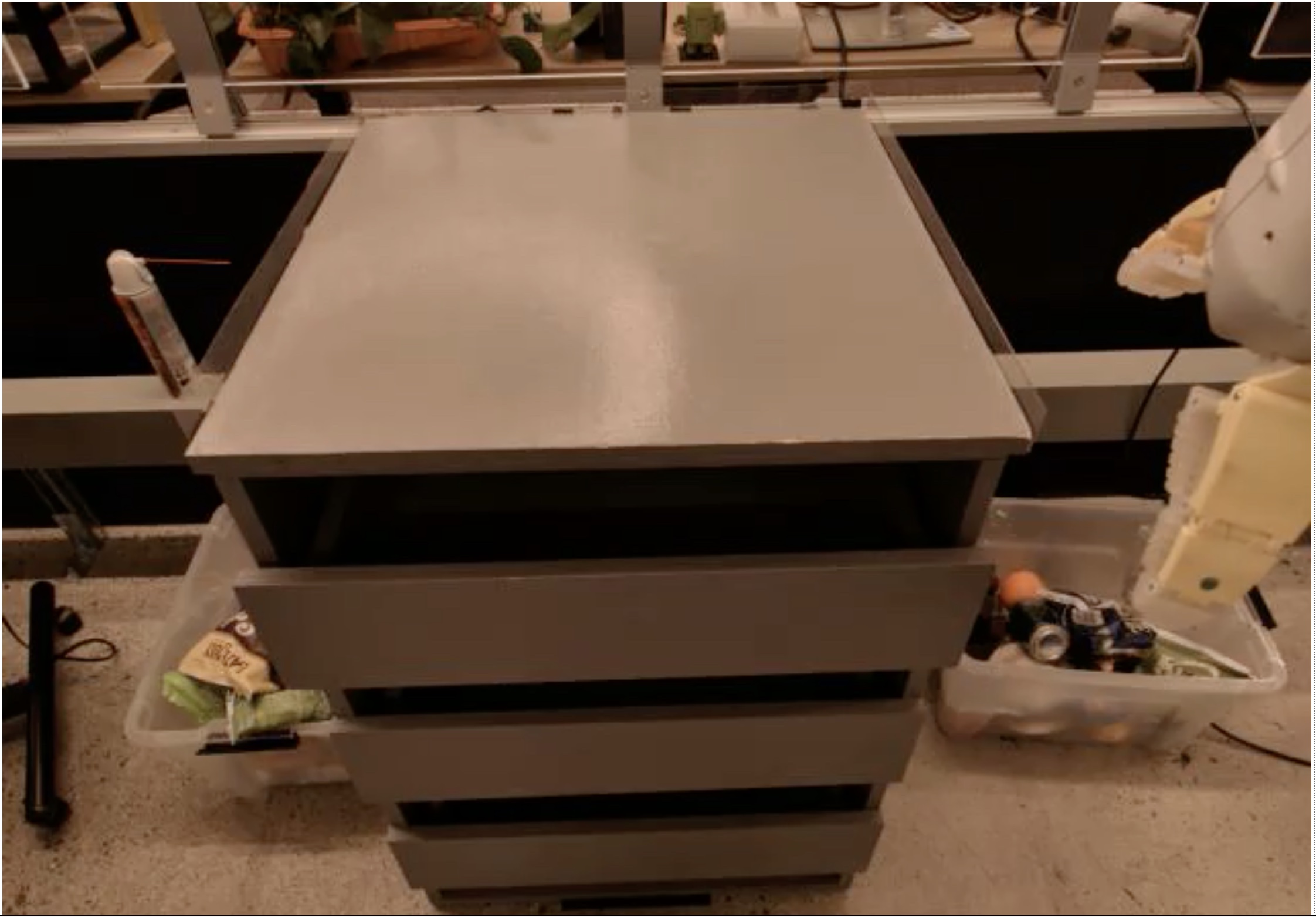
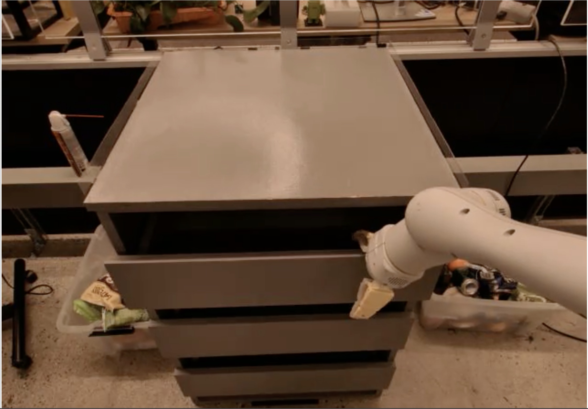
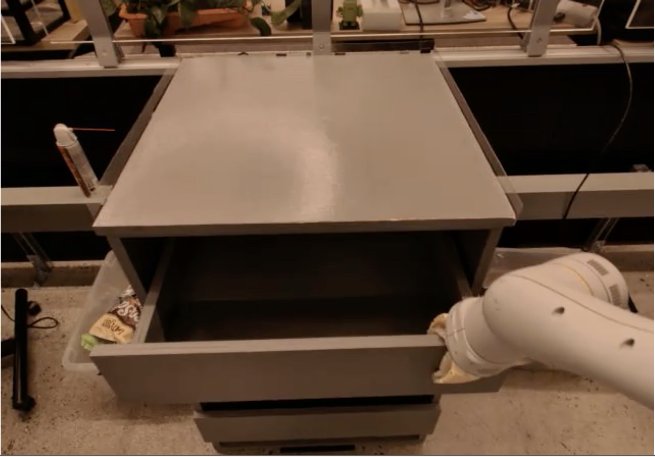
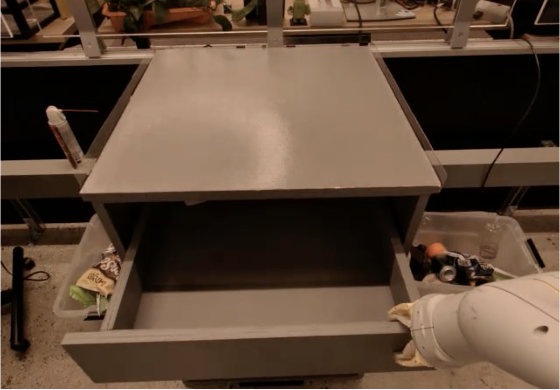
Figure 4: Example input frames from the robot task “pick pepsi can” (top) and “open top drawer” (bottom). We learn one action policy, which needs to cover all 551 task instructions.

4.1.5 Spatio-temporal Activity Detection Results

We conducted an additional experiment on AVA [32] to confirm the benefit of TTM. We followed the lightest setting of pretraining the backbone with Kinetics-400. Identical to our Charades experiments, ViViT-B was used as the backbone. The only difference is that it was trained by providing video segments of 4 steps (i.e., $32\times 4$ frames) at a time, due to the memory constraint. The bounding box proposals are obtained with the SlowFast network [27], and the TTM was responsible for computing the feature mask to be pooled per bounding box.

Table 6 compares the TTM with its backbone. We are able to observe the benefit of TTM, which improves the accuracy by managing the external memory, with a little added compute. We also provided its comparison against MeMViT [66], which also presents a Transformer-based memory mechanism for sequential visual data. Note that there are various ways to further boost the accuracy numbers orthogonal to the proposed sequential modeling. This includes the use of larger pretraining dataset [66], use of bigger backbones [66, 63], and better pretraining with self-supervised losses [63]. What we confirm in this experiment is the relative gain over the backbone; TTM with a small added compute, by utilizing the memory, improves AVA activity detection.

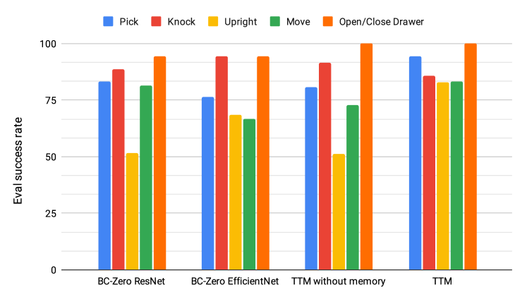
Figure 5: Real robot experiment; per-task success rates.

Model	Success
BC ResNet	79.80
BC EfficientNet	80.08
No memory	79.26
TTM	89.26

Figure 6: Average task success rate in real-robot evaluation.

4.2 Robot Learning

To study how TTM scales to a real-world robotic control setting, we integrate it to a real kitchen environment described in SayCan [1]. An Everyday Robots robot, a mobile manipulator with RGB observations, is placed in an office kitchen to interact with common objects using concurrent [68] continuous closed-loop control from pixels. Here, at each time step, the inputs to the model are an image from the robot’s mounted camera and the task instruction in natural language (Fig. 4). The expected output is an action vector for robot arm and base control. The policy was trained under a supervised behavioral cloning (BC) setting with human demonstrations.

4.2.1 Dataset and Settings

We use the dataset and settings as described in SayCan [1] with the additional inclusion of controls for base motion. We collect the dataset to train imitation learning policies: a real-world dataset of teleoperated human demonstrations of successful policy rollouts filtered by engineered success detectors. Such real2real setup includes a training dataset of 89,000 teleoperated episodes collected in a mock kitchen across 551 tasks involving skills like picking, placing, and manipulating furniture. Each task instruction (with different objects) were given in the form of a text sentence, and the robot was asked to learn a single model for all such tasks. A policy trained on the dataset is evaluated again in the same kitchen in real-time. The tasks are grouped into 5 different types, Pick, Knock, Upright, Move, and Open/Close Drawer, and we report success rate of each type.

4.2.2 Baselines and Implementation

We follow the learning framework described in SayCan  [1]. Here the first baseline we benchmark against is the ResNet based control policy network, called BC-Zero ResNet, developed in  [38] and used in SayCan. A second baseline we consider is BC-Zero with the image trunk swapped for a pretrained EfficientNet [59], while still applying FiLM conditioning  [51] for language as described in [38] for ResNet. We call this the BC-Zero EfficientNet. EfficientNet is computationally more efficient and pretraining on ImageNet improves object understanding.

Against these baselines we benchmark the proposed TTM architecture. TTM treats EfficientNet outputs as the input tokens. The memory size of TTM was $m=96$, the number of reads was $r=16$, and $n=48$ after aggregation. A Transformer with 8 layers was used as the processing unit by default, and the total of 8 steps were considered at a time. We also compare TTM against its memory-less version, which uses the same framework and the compute to the TTM. The only difference is that the memory has been zeroed out.

4.3 Real-robot Results

We compare TTM against the baselines discussed above including BC-Zero used in SayCan. Inputs to the models are images from the robot’s mounted headcam, previous actions executed in the episode and natural language instruction for the task. Outputs are action vectors to control the robot in real evaluation, as discussed in Section 4.2.1.

Fig. 6 and Table 6 show the results. We observe significant improvements with TTM in the task success rate, since knowledge of previous history is critical for this task. Fig. 4 shows frames from the real robot in operation.

5 Conclusion

We introduce Token Turing Machines for sequential decision making. Token Turing Machines could be viewed as a modernisation of Neural Turing Machines, with memory reads/writes designed in terms of token summarisations. It has good perks of modern Transformer-based models while also benefiting from having an external memory: constant compute regardless of the length of the history. Such capability is particularly important in many sequential decision making and online inference problems, such as robot action policy learning. We confirmed its power on real-world tasks with challenging visual inputs: Charades activity localization, and vision-based robot action policy learning.

Discussions:

The applicability of TTMs themselves is broad, as they are generic sequential models designed to digest a large number of tokens. Our intention with this paper particularly has been to focus on computer vision problems with sequential visual data. The problems that we chose (i.e., spatio-temporal human action localisation and robot policy) are challenging as they require extremely long sequences of tokens: For our experiments on action localisation, we have 3136 tokens per step, multiplied by 6 steps, which is a total of 18816 tokens. This sequence length is therefore significantly larger than those in other domains and comparable to Long Range Arena [60] (1000 to 16000 tokens), posing comparable yet different challenges.

We also emphasize that TTM is the first to show its applicability to videos among the NTM-based approaches.

Appendix A Appendix

A.1 Charades Training

For Charades [57] training, we initialize ViViT [3] backbones with pretrained weights (Base model: JFT [58] $\rightarrow$ Kinetics-400 [42], Large model: JFT $\rightarrow$ Kinetics-600 [9]) and initialize TTM-head with random weights. We finetune models with a batch size of 32 and Adam optimizer [44] with an initial learning rate of 1e-4 (with backbone learning rate further scaled by 0.1) and a cosine schedule for 100 epochs on 32 TPUv3 cores. To prevent overfitting, we use color/scale jitter, random augmentations [15] and mixup [72]. Our implementation is based on Jax [6] and the Scenic library [20]. We use sigmoid cross-entropy loss with a label smoothing of 0.1. Our inputs contain 6 temporal steps, each with 32 frames of 224$\times$224 resolution, and the loss is applied to the last step only. This allows better training for the TTM memory module.

A.2 Robot Policy Training

In our robot experiments, all architectures are trained in a behavioral cloning setting on the real2real dataset described in Section 4.2.1. For the training of the policy, we follow experimental setup of SayCan [1].

References

- [1] Michael Ahn, Anthony Brohan, Noah Brown, Yevgen Chebotar, Omar Cortes, Byron David, Chelsea Finn, Keerthana Gopalakrishnan, Karol Hausman, Alex Herzog, Daniel Ho, Jasmine Hsu, Julian Ibarz, Brian Ichter, Alex Irpan, Eric Jang, Rosario Jauregui Ruano, Kyle Jeffrey, Sally Jesmonth, Nikhil Joshi, Ryan Julian, Dmitry Kalashnikov, Yuheng Kuang, Kuang-Huei Lee, Sergey Levine, Yao Lu, Linda Luu, Carolina Parada, Peter Pastor, Jornell Quiambao, Kanishka Rao, Jarek Rettinghouse, Diego Reyes, Pierre Sermanet, Nicolas Sievers, Clayton Tan, Alexander Toshev, Vincent Vanhoucke, Fei Xia, Ted Xiao, Peng Xu, Sichun Xu, and Mengyuan Yan. Do as i can and not as i say: Grounding language in robotic affordances. In arXiv preprint arXiv:2204.01691, 2022.
- [2] Hassan Akbari, Liangzhe Yuan, Rui Qian, Wei-Hong Chuang, Shih-Fu Chang, Yin Cui, and Boqing Gong. Vatt: Transformers for multimodal self-supervised learning from raw video, audio and text. Advances in Neural Information Processing Systems, 34:24206–24221, 2021.
- [3] Anurag Arnab, Mostafa Dehghani, Georg Heigold, Chen Sun, Mario Lučić, and Cordelia Schmid. Vivit: A video vision transformer. In ICCV, 2021.
- [4] Gedas Bertasius, Heng Wang, and Lorenzo Torresani. Is space-time attention all you need for video understanding? In ICML, volume 2, page 4, 2021.
- [5] Sebastian Borgeaud, Arthur Mensch, Jordan Hoffmann, Trevor Cai, Eliza Rutherford, Katie Millican, George Bm Van Den Driessche, Jean-Baptiste Lespiau, Bogdan Damoc, Aidan Clark, et al. Improving language models by retrieving from trillions of tokens. In International Conference on Machine Learning, 2022.
- [6] James Bradbury, Roy Frostig, Peter Hawkins, Matthew James Johnson, Chris Leary, Dougal Maclaurin, George Necula, Adam Paszke, Jake VanderPlas, Skye Wanderman-Milne, and Qiao Zhang. JAX: composable transformations of Python+NumPy programs, 2018.
- [7] Mikhail S Burtsev, Yuri Kuratov, Anton Peganov, and Grigory V Sapunov. Memory transformer. arXiv preprint arXiv:2006.11527, 2020.
- [8] Fabian Caba Heilbron, Victor Escorcia, Bernard Ghanem, and Juan Carlos Niebles. Activitynet: A large-scale video benchmark for human activity understanding. In Proceedings of the ieee conference on computer vision and pattern recognition, pages 961–970, 2015.
- [9] Joao Carreira, Eric Noland, Andras Banki-Horvath, Chloe Hillier, and Andrew Zisserman. A short note about kinetics-600, 2018.
- [10] Joao Carreira and Andrew Zisserman. Quo vadis, action recognition? a new model and the kinetics dataset. In proceedings of the IEEE Conference on Computer Vision and Pattern Recognition, pages 6299–6308, 2017.
- [11] Rewon Child, Scott Gray, Alec Radford, and Ilya Sutskever. Generating long sequences with sparse transformers. arXiv preprint arXiv:1904.10509, 2019.
- [12] Krzysztof Choromanski, Valerii Likhosherstov, David Dohan, Xingyou Song, Andreea Gane, Tamas Sarlos, Peter Hawkins, Jared Davis, Afroz Mohiuddin, Lukasz Kaiser, et al. Rethinking attention with performers. arXiv preprint arXiv:2009.14794, 2020.
- [13] Junyoung Chung, Caglar Gulcehre, KyungHyun Cho, and Yoshua Bengio. Empirical evaluation of gated recurrent neural networks on sequence modeling. arXiv preprint arXiv:1412.3555, 2014.
- [14] Jean-Baptiste Cordonnier, Aravindh Mahendran, Alexey Dosovitskiy, Dirk Weissenborn, Jakob Uszkoreit, and Thomas Unterthiner. Differentiable patch selection for image recognition. In CVPR, 2021.
- [15] Ekin D Cubuk, Barret Zoph, Jonathon Shlens, and Quoc V Le. Randaugment: Practical automated data augmentation with a reduced search space. In Proceedings of the IEEE/CVF conference on computer vision and pattern recognition workshops, pages 702–703, 2020.
- [16] Rui Dai, Srijan Das, and Francois Bremond. Ctrn: Class temporal relational network for action detection. In BMVC 2021-The British Machine Vision Conference, 2021.
- [17] Rui Dai, Srijan Das, Kumara Kahatapitiya, Michael S Ryoo, and Francois Bremond. Ms-tct: Multi-scale temporal convtransformer for action detection. In Proceedings of the IEEE/CVF Conference on Computer Vision and Pattern Recognition, pages 20041–20051, 2022.
- [18] Rui Dai, Srijan Das, Luca Minciullo, Lorenzo Garattoni, Gianpiero Francesca, and Francois Bremond. Pdan: Pyramid dilated attention network for action detection. In Proceedings of the IEEE/CVF Winter Conference on Applications of Computer Vision, pages 2970–2979, 2021.
- [19] Zihang Dai, Zhilin Yang, Yiming Yang, Jaime Carbonell, Quoc V Le, and Ruslan Salakhutdinov. Transformer-xl: Attentive language models beyond a fixed-length context. In ACL, 2019.
- [20] Mostafa Dehghani, Alexey Gritsenko, Anurag Arnab, Matthias Minderer, and Yi Tay. Scenic: A jax library for computer vision research and beyond. In Proceedings of the IEEE/CVF Conference on Computer Vision and Pattern Recognition (CVPR), pages 21393–21398, 2022.
- [21] Aniket Didolkar, Kshitij Gupta, Anirudh Goyal, Nitesh B. Gundavarapu, Alex Lamb, Nan Rosemary Ke, and Yoshua Bengio. Temporal latent bottleneck: Synthesis of fast and slow processing mechanisms in sequence learning. In NeurIPS, 2022.
- [22] Jeffrey Donahue, Lisa Anne Hendricks, Sergio Guadarrama, Marcus Rohrbach, Subhashini Venugopalan, Kate Saenko, and Trevor Darrell. Long-term recurrent convolutional networks for visual recognition and description. In CVPR, June 2015.
- [23] Alexey Dosovitskiy, Lucas Beyer, Alexander Kolesnikov, Dirk Weissenborn, Xiaohua Zhai, Thomas Unterthiner, Mostafa Dehghani, Matthias Minderer, Georg Heigold, Sylvain Gelly, Jakob Uszkoreit, and Neil Houlsby. An image is worth 16x16 words: Transformers for image recognition at scale. arXiv preprint arXiv:2010.11929, 2020.
- [24] Haoqi Fan, Bo Xiong, Karttikeya Mangalam, Yanghao Li, Zhicheng Yan, Jitendra Malik, and Christoph Feichtenhofer. Multiscale vision transformers. In Proceedings of the IEEE/CVF International Conference on Computer Vision, pages 6824–6835, 2021.
- [25] Mohsen Fayyaz, Soroush Abbasi Koohpayegani, Farnoush Rezaei Jafari, Sunando Sengupta, Hamid Reza Vaezi Joze, Eric Sommerlade, Hamed Pirsiavash, and Juergen Gall. Adaptive token sampling for efficient vision transformers. In ECCV, 2022.
- [26] Christoph Feichtenhofer. X3D: Expanding architectures for efficient video recognition. In Proceedings of the IEEE/CVF Conference on Computer Vision and Pattern Recognition, pages 203–213, 2020.
- [27] Christoph Feichtenhofer, Haoqi Fan, Jitendra Malik, and Kaiming He. Slowfast networks for video recognition. In Proceedings of the IEEE/CVF international conference on computer vision, pages 6202–6211, 2019.
- [28] Pallabi Ghosh, Yi Yao, Larry Davis, and Ajay Divakaran. Stacked spatio-temporal graph convolutional networks for action segmentation. In The IEEE Winter Conference on Applications of Computer Vision, pages 576–585, 2020.
- [29] Anirudh Goyal, Aniket Didolkar, Alex Lamb, Kartikeya Badola, Nan Rosemary Ke, Nasim Rahaman, Jonathan Binas, Charles Blundell, Michael Mozer, and Yoshua Bengio. Coordination among neural modules through a shared global workspace. In ICLR, 2022.
- [30] Alex Graves, Greg Wayne, and Ivo Danihelka. Neural Turing machines. arXiv preprint arXiv:1410.5401, 2014.
- [31] Alex Graves, Greg Wayne, Malcolm Reynolds, Tim Harley, Ivo Danihelka, Agnieszka Grabska-Barwińska, Sergio Gómez Colmenarejo, Edward Grefenstette, Tiago Ramalho, John Agapiou, et al. Hybrid computing using a neural network with dynamic external memory. Nature, 538(7626):471–476, 2016.
- [32] Chunhui Gu, Chen Sun, David A Ross, Carl Vondrick, Caroline Pantofaru, Yeqing Li, Sudheendra Vijayanarasimhan, George Toderici, Susanna Ricco, Rahul Sukthankar, et al. Ava: A video dataset of spatio-temporally localized atomic visual actions. In Proceedings of the IEEE Conference on Computer Vision and Pattern Recognition, pages 6047–6056, 2018.
- [33] Kelvin Guu, Kenton Lee, Zora Tung, Panupong Pasupat, and Mingwei Chang. Retrieval augmented language model pre-training. In International Conference on Machine Learning, 2020.
- [34] Sepp Hochreiter, Yoshua Bengio, Paolo Frasconi, Jürgen Schmidhuber, et al. Gradient flow in recurrent nets: the difficulty of learning long-term dependencies, 2001.
- [35] Sepp Hochreiter and Jürgen Schmidhuber. Long short-term memory. Neural computation, 9(8):1735–1780, 1997.
- [36] DeLesley Hutchins, Imanol Schlag, Yuhuai Wu, Ethan Dyer, and Behnam Neyshabur. Block-recurrent transformers. In NeurIPS, 2022.
- [37] Andrew Jaegle, Felix Gimeno, Andy Brock, Oriol Vinyals, Andrew Zisserman, and Joao Carreira. Perceiver: General perception with iterative attention. In ICML, 2021.
- [38] Eric Jang, Alex Irpan, Mohi Khansari, Daniel Kappler, Frederik Ebert, Corey Lynch, Sergey Levine, and Chelsea Finn. Bc-z: Zero-shot task generalization with robotic imitation learning. 2022.
- [39] Kumara Kahatapitiya, Zhou Ren, Haoxiang Li, Zhenyu Wu, and Michael S Ryoo. Self-supervised pretraining with classification labels for temporal activity detection. arXiv preprint arXiv:2111.13675, 2021.
- [40] Kumara Kahatapitiya and Michael S Ryoo. Coarse-fine networks for temporal activity detection in videos. In Proceedings of the IEEE/CVF Conference on Computer Vision and Pattern Recognition, pages 8385–8394, 2021.
- [41] Łukasz Kaiser, Ofir Nachum, Aurko Roy, and Samy Bengio. Learning to remember rare events. arXiv preprint arXiv:1703.03129, 2017.
- [42] Will Kay, Joao Carreira, Karen Simonyan, Brian Zhang, Chloe Hillier, Sudheendra Vijayanarasimhan, Fabio Viola, Tim Green, Trevor Back, Paul Natsev, Mustafa Suleyman, and Andrew Zisserman. The kinetics human action video dataset, 2017.
- [43] Urvashi Khandelwal, Omer Levy, Dan Jurafsky, Luke Zettlemoyer, and Mike Lewis. Generalization through memorization: Nearest neighbor language models. arXiv preprint arXiv:1911.00172, 2019.
- [44] Diederik P Kingma and Jimmy Ba. Adam: A method for stochastic optimization. arXiv preprint arXiv:1412.6980, 2014.
- [45] Hung Le, Truyen Tran, and Svetha Venkatesh. Learning to remember more with less memorization. arXiv preprint arXiv:1901.01347, 2019.
- [46] Ze Liu, Yutong Lin, Yue Cao, Han Hu, Yixuan Wei, Zheng Zhang, Stephen Lin, and Baining Guo. Swin transformer: Hierarchical vision transformer using shifted windows. In Proceedings of the IEEE/CVF International Conference on Computer Vision, pages 10012–10022, 2021.
- [47] Ze Liu, Jia Ning, Yue Cao, Yixuan Wei, Zheng Zhang, Stephen Lin, and Han Hu. Video swin transformer. In Proceedings of the IEEE/CVF Conference on Computer Vision and Pattern Recognition, pages 3202–3211, 2022.
- [48] Effrosyni Mavroudi, Benjamín Béjar Haro, and René Vidal. Representation learning on visual-symbolic graphs for video understanding. In European Conference on Computer Vision, pages 71–90. Springer, 2020.
- [49] Arsha Nagrani, Shan Yang, Anurag Arnab, Aren Jansen, Cordelia Schmid, and Chen Sun. Attention bottlenecks for multimodal fusion. Advances in Neural Information Processing Systems, 34:14200–14213, 2021.
- [50] Hao Peng, Nikolaos Pappas, Dani Yogatama, Roy Schwartz, Noah A Smith, and Lingpeng Kong. Random feature attention. arXiv preprint arXiv:2103.02143, 2021.
- [51] Ethan Perez, Florian Strub, Harm de Vries, Vincent Dumoulin, and Aaron C. Courville. Film: Visual reasoning with a general conditioning layer. CoRR, abs/1709.07871, 2017.
- [52] AJ Piergiovanni and Michael S Ryoo. Learning latent super-events to detect multiple activities in videos. In Proceedings of the IEEE Conference on Computer Vision and Pattern Recognition, pages 5304–5313, 2018.
- [53] AJ Piergiovanni and Michael S. Ryoo. Temporal gaussian mixture layer for videos. In International Conference on Machine learning, pages 5152–5161, 2019.
- [54] Jack W Rae, Anna Potapenko, Siddhant M Jayakumar, and Timothy P Lillicrap. Compressive transformers for long-range sequence modelling. arXiv preprint arXiv:1911.05507, 2019.
- [55] Yongming Rao, Wenliang Zhao, Benlin Liu, Jiwen Lu, Jie Zhou, and Cho-Jui Hsieh. Dynamicvit: Efficient vision transformers with dynamic token sparsification. In NeurIPS, 2021.
- [56] Michael Ryoo, AJ Piergiovanni, Anurag Arnab, Mostafa Dehghani, and Anelia Angelova. Tokenlearner: Adaptive space-time tokenization for videos. In NeurIPS, 2021.
- [57] Gunnar A Sigurdsson, Gül Varol, Xiaolong Wang, Ali Farhadi, Ivan Laptev, and Abhinav Gupta. Hollywood in homes: Crowdsourcing data collection for activity understanding. In European Conference on Computer Vision, pages 510–526. Springer, 2016.
- [58] Chen Sun, Abhinav Shrivastava, Saurabh Singh, and Abhinav Gupta. Revisiting unreasonable effectiveness of data in deep learning era. In Proceedings of the IEEE international conference on computer vision, pages 843–852, 2017.
- [59] Mingxing Tan and Quoc Le. Efficientnet: Rethinking model scaling for convolutional neural networks. In International conference on machine learning, pages 6105–6114. PMLR, 2019.
- [60] Yi Tay, Mostafa Dehghani, Samira Abnar, Yikang Shen, Dara Bahri, Philip Pham, Jinfeng Rao, Liu Yang, Sebastian Ruder, and Donald Metzler. Long range arena: A benchmark for efficient transformers. arXiv preprint arXiv:2011.04006, 2020.
- [61] Yi Tay, Mostafa Dehghani, Dara Bahri, and Donald Metzler. Efficient transformers: A survey. ACM Computing Surveys (CSUR), 2022.
- [62] Ilya Tolstikhin, Neil Houlsby, Alexander Kolesnikov, Lucas Beyer, Xiaohua Zhai, Thomas Unterthiner, Jessica Yung, Andreas Steiner, Daniel Keysers, Jakob Uszkoreit, Mario Lucic, and Alexey Dosovitskiy. Mlp-mixer: An all-mlp architecture for vision. In NeurIPS, 2021.
- [63] Zhan Tong, Yibing Song, Jue Wang, and Limin Wang. Videomae: Masked autoencoders are data-efficient learners for self-supervised video pre-training. arXiv preprint arXiv:2203.12602, 2022.
- [64] Ashish Vaswani, Noam Shazeer, Niki Parmar, Jakob Uszkoreit, Llion Jones, Aidan N Gomez, Łukasz Kaiser, and Illia Polosukhin. Attention is all you need. In NeurIPS, 2017.
- [65] Sinong Wang, Belinda Z Li, Madian Khabsa, Han Fang, and Hao Ma. Linformer: Self-attention with linear complexity. arXiv preprint arXiv:2006.04768, 2020.
- [66] Chao-Yuan Wu, Yanghao Li, Karttikeya Mangalam, Haoqi Fan, Bo Xiong, Jitendra Malik, and Christoph Feichtenhofer. Memvit: Memory-augmented multiscale vision transformer for efficient long-term video recognition. In CVPR, 2022.
- [67] Yuhuai Wu, Markus N Rabe, DeLesley Hutchins, and Christian Szegedy. Memorizing transformers. In ICLR, 2022.
- [68] Ted Xiao, Eric Jang, Dmitry Kalashnikov, Sergey Levine, Julian Ibarz, Karol Hausman, and Alexander Herzog. Thinking while moving: Deep reinforcement learning with concurrent control. arXiv preprint arXiv:2004.06089, 2020.
- [69] Serena Yeung, Olga Russakovsky, Ning Jin, Mykhaylo Andriluka, Greg Mori, and Li Fei-Fei. Every moment counts: Dense detailed labeling of actions in complex videos. International Journal of Computer Vision, 126(2-4):375–389, 2018.
- [70] Hongxu Yin, Arash Vahdat, Jose M Alvarez, Arun Mallya, Jan Kautz, and Pavlo Molchanov. A-vit: Adaptive tokens for efficient vision transformer. In CVPR, 2022.
- [71] Manzil Zaheer, Guru Guruganesh, Kumar Avinava Dubey, Joshua Ainslie, Chris Alberti, Santiago Ontanon, Philip Pham, Anirudh Ravula, Qifan Wang, Li Yang, et al. Big bird: Transformers for longer sequences. Advances in Neural Information Processing Systems, 33:17283–17297, 2020.
- [72] Hongyi Zhang, Moustapha Cisse, Yann N Dauphin, and David Lopez-Paz. mixup: Beyond empirical risk minimization. arXiv preprint arXiv:1710.09412, 2017.