Light-induced phase crossovers in a quantum spin Hall system

Abstract

In this work, we theoretically investigate the light-induced topological phases and finite-size crossovers in a paradigmatic quantum spin Hall (QSH) system with high-frequency pumping optics. Taking the HgTe quantum well for an example, our numerical results show that circularly polarized light can break time-reversal symmetry and induce the quantum anomalous Hall (QAH) phase. In particular, the coupling between the edge states is spin dependent and is related not only to the size of the system, but also to the strength of the polarized pumping optics. By tuning the two parameters (system width and optical pumping strength), we obtain four transport regimes, namely, QSH, QAH, edge conducting, and normal insulator. These four different transport regimes have contrasting edge conducting properties, which will feature prominently in transport experiments on various topological materials.

I Introduction

The quantum spin Hall (QSH) insulator is a member of the family of quantum Hall insulators first proposed by Kane and Mele Kane and Mele (2005a, b). It is an energy band insulator in bulk, but conducting at the edges Abergel (2018). The edges carry two different charge currents with spin-up and spin-down moving in opposite directions. A more realistic version of the QSH effect in HgTe quantum wells was proposed by Bernevig, Hughes, and Zhang Bernevig et al. (2006) and was soon confirmed by experiment Konig et al. (2007); König et al. (2008). Since then, there have been intensive studies to investigate the exotic properties in QSH systems Prodan (2009). They include topological field theory Qi et al. (2008); Yu et al. (2011); Lee and Ye (2015), finite-size crossovers in topological insulators Zhou et al. (2008); Liu et al. (2010), magnetic doping in QSH system (Mn-doped HgTe quantum well) Fu et al. (2014), disorder-induced topological Anderson insulator in QSH systems Li et al. (2009); Jiang et al. (2009); Groth et al. (2009); Xing et al. (2011); Li et al. (2011); Ning et al. (2022), Floquet topological insulator states in QSH systems Calvo et al. (2015); Zhu et al. (2014); Qin et al. (2022a); Liu et al. (2021), as well as QSH effects in three-dimensional topological insulators Li et al. (2010); Dabiri et al. (2021); Dabiri and Cheraghchi (2021); Pervishko et al. (2018); Zhu et al. (2022).

The quantum anomalous Hall (QAH) insulator, which was first proposed by Haldane Haldane (1988), is another key member of the family of quantum Hall insulators. A QAH insulator can have a quantized Hall conductivity even without an external magnetic field that breaks the time-reversal symmetry Haldane (1988); Chang et al. (2013); Yu et al. (2010); Linder et al. (2009); Lu et al. (2013, 2010); Shan et al. (2010). The QAH effect was first experimentally observed in Ref. Chang et al. (2013); in another work on finite-size effects in QAH systems Fu et al. (2014), they adopted the magnetic doping (Mn doping) to break the time-reversal symmetry and introduce the QAH phase in the HgTe quantum well. By appropriate tuning of the doping concentration and the system size, they have obtained a variety of topological phases Fu et al. (2014).

Yet, this experimental success Fu et al. (2014) in realizing QAH states proved difficult to follow up since the doping concentration is difficult to tune continuously in experiments. Therefore, departing from previous works Fu et al. (2014), we shall provide a more experimentally accessible alternative to realizing QAH states, using circularly polarized light instead of magnetic doping to break the time-reversal symmetry in HgTe quantum well. This hinges on the fact that the intensity of circularly polarized light can be easily tuned continuously in experiments, and that Floquet driving can induce a host of exotic phases in various media, such as disorder-induced Floquet topological insulators Titum et al. (2015), quenched topological boundary modes induced by Floquet engineering Lee and Song (2021), Floquet semimetal with exotic topological linkages Li et al. (2018), Floquet mechanism for non-Abelian fractional quantum Hall states Lee et al. (2018), photoinduced half-integer quantized conductance plateaus in topological insulators Yap et al. (2018), and tunable Floquet-Weyl semimetals driven from nodal line semimetals Chan et al. (2016); Bonasera et al. (2022). In this work, based on numerical calculations with high-frequency Floquet expansion, we find that circularly polarized light can break the time-reversal symmetry and introduce the QAH phase in a HgTe quantum well. Our findings complement other works that utilize circularly polarized light to induce new topological phases in graphene Oka and Aoki (2009); Sato et al. (2019); McIver et al. (2020); Sentef et al. (2015); Broers and Mathey (2022); Candussio et al. (2022); Qin et al. (2022b); Cupo et al. (2021); Assi et al. (2021); Luo (2021); Schüler et al. (2020); Topp et al. (2019); Rodriguez-Vega et al. (2020); Li et al. (2020); Berdakin et al. (2021); Dal Lago et al. (2017); Huamán et al. (2021), but with significant differences. In particular, the coupling between the edge states is spin dependent and is related not only to the width of the system, but also to the strength of the polarized pumping optics. By appropriate tuning of the system size and strength of the pumping optics, we obtain four transport regimes including QSH, QAH, edge conducting (EC), and normal insulator (NI).

The paper is organized as follows. In Section II, we introduce the model Hamiltonian that we use. In Section III, we derive the corresponding Floquet effective Hamiltonian by using the high-frequency expansions. In Section IV, we calculate the energy dispersions under the open boundary condition along the $y$ direction and periodic boundary conditions along the $x$ direction with fixed light intensity and different system size by numerically diagonalizing the corresponding tight-binding Hamiltonian. In Section V, we give and discuss our phase diagram. Finally, we summarize our results in Section VI.

II Model

We start with the Bernevig-Hughes-Zhang (BHZ) model given by the low-energy two-dimensional effective Hamiltonian near the $\Gamma$ point to describe the electronic states in HgTe/(Hg,Cd)Te quantum wells Bernevig et al. (2006); Konig et al. (2007); König et al. (2008); Zhou et al. (2008); Rothe et al. (2010); Zhu et al. (2014)

$${\cal H}({\bf k}) =\begin{pmatrix}h({\bf k})&0\\ 0&h^{*}(-{\bf k})\end{pmatrix}$$

$$=\epsilon_{\bf k}\tau_{0}\otimes\sigma_{0}+Ak_{x}\tau_{z}\otimes\sigma_{x}+Ak_{y}\tau_{0}\otimes\sigma_{y}$$

$$+{\cal M}_{\bf k}\tau_{0}\otimes\sigma_{z},$$ (1)

where $h({\bf k})=\epsilon_{\bf k}\sigma_{0}+Ak_{x}\sigma_{x}+Ak_{y}\sigma_{y}+{\cal M}_{\bf k}\sigma_{z}$, $h^{*}(-{\bf k})=\epsilon_{\bf k}\sigma_{0}-Ak_{x}\sigma_{x}-Ak_{y}\sigma_{y}^{*}+{\cal M}_{\bf k}\sigma_{z}$, $\epsilon_{\bf k}=C-Dk^{2}$, ${\cal M}_{\bf k}=M-Bk^{2}$, $k^{2}=k_{x}^{2}+k_{y}^{2}$, $A$, $B$, $C$, $D$, and $M$ are the material specific parameters, ${\bf k}=(k_{x},k_{y})$, $k_{x}$ and $k_{y}$ are the momenta of two-dimensional electron gas, $\sigma_{x,y,z}$ ($\tau_{x,y,z}$) are the Pauli matrices, and $\sigma_{0}$ ($\tau_{0}$) is the $2\times 2$ identity matrix. The parameters are adopted as König et al. (2008) $A=364.5$ meV$\cdot$nm, $B=-686$ meV$\cdot$nm², $D=-512$ meV$\cdot$nm², $M=-10$ meV. Without loss of generality, we assume that $C=0$.

In particular, the $h({\bf k})$ and $h^{*}(-{\bf k})$ in the matrix diagonal blocks of Eq. (II) provide the simplest ansatz that ensures time inversion symmetry in the model Hamiltonian. In addition, $h({\bf k})$ and $h^{*}(-{\bf k})$ are equivalent to the two-dimensional Dirac model or Qi-Wu-Zhang (QWZ) model Qi et al. (2006); Qi and Zhang (2011); Chen et al. (2019), which has a quantized Hall conductance without Landau levels. Thus, $h({\bf k})$ and $h^{*}(-{\bf k})$ correspond to two equal but opposite QAH Hamiltonians. Therefore, the net Hall conductance of the Hamiltonian (II) is zero, but the spin Hall conductance for $h({\bf k})$ or $h^{*}(-{\bf k})$ is nonzero. This phenomenon corresponds to the QSH state. The BHZ model can be viewed as two copies of QWZ models with opposite Hall conductance.

III Floquet Hamiltonian

To realize QAH states in the Hamiltonian (II), circularly polarized light can be used to break the time-reversal symmetry between the two spin blocks of the matrix (II) to result in nonzero net Hall conductance.

The optical driving field can be expressed as ${\bf E}(t)=\partial{\bf A}(t)/\partial t=E(\cos(\omega t),\cos(\omega t+\varphi),0)$, where ${\bf A}(t)={\bf A}(t+T)$ is the time periodic vector potential with period $T=2\pi/\omega$, $\omega$ is the frequency of the optical field, and $E$ is the amplitude of the optical field. The optical field is circularly polarized with $\varphi=\pm\pi/2$ and ${\bf A}(t)=A_{a}(\sin(\omega t),\pm\cos(\omega t),0)$, where $A_{a}=E/\omega$ and $\pm$ corresponds to right- and left-handed circularly polarized waves, respectively. To guarantee the off-resonant regime in which the central Floquet band is far away from other replicas, the driven frequency can be set as $\hbar\omega=150$ meV, which is much larger than the bandwidth Trevisan et al. (2022); Qin et al. (2022a); Dabiri et al. (2021); Dabiri and Cheraghchi (2021); Pervishko et al. (2018).

After irradiation with light, the photon-dressed effective Hamiltonian is given by

$${\cal H}({\bf k},t)={\cal H}\left({\bf k}-\frac{e}{\hbar}{\bf A}(t)\right).$$ (2)

Within the Floquet theory Oka and Aoki (2009); Calvo et al. (2015); Chen et al. (2018a, b); Du et al. (2022); Ning et al. (2022); Qin et al. (2022a); Wang et al. (2022); Jangjan and Hosseini (2020, 2021) and $A_{0}=eA_{a}/\hbar$ which denotes the light intensity, the effective static Hamiltonian in the high-frequency regime can be expanded as

$${\cal H}^{(F)}={\cal H}_{0,0}+\frac{[{\cal H}_{0,-1},{\cal H}_{0,1}]}{\hbar\omega},$$ (3)

where we use ${\cal H}_{n,m}=\frac{1}{T}\int_{0}^{T}{\cal H}({\bf k},t)e^{i(n-m)\omega t}dt$ with $n$ and $m$ as integers, and the concrete analytical expressions for ${\cal H}_{0,0}$, ${\cal H}_{0,-1}$, and ${\cal H}_{0,1}$ can be found in Appendix A.

From Eq. (3), the Floquet Hamiltonian is given by

$${\cal H}^{(F)}({\bf k}) \!=\!\begin{pmatrix}h_{\uparrow}({\bf k})&0\\ 0&h_{\downarrow}({\bf k})\end{pmatrix},$$ (4)

where $h_{\uparrow}({\bf k})\!=\!-D(A_{0}^{2}+k^{2})\sigma_{0}\!+\!\left(\!\tilde{M}_{\uparrow}\!-\!Bk^{2}\!\right)\!\sigma_{z}\!+\!\tilde{A}_{\uparrow}(k_{x}\sigma_{x}\!+\!k_{y}\sigma_{y})$, $h_{\downarrow}({\bf k})\!=\!-D(A_{0}^{2}+k^{2})\sigma_{0}\!+\!\left(\!\tilde{M}_{\downarrow}\!-\!Bk^{2}\!\right)\!\sigma_{z}\!-\!\tilde{A}_{\downarrow}(k_{x}\sigma_{x}\!-\!k_{y}\sigma_{y})$, $\tilde{A}_{\uparrow}\!=\!\left[\!1\!-\!2A_{0}^{2}B\sin\varphi/(\hbar\omega)\!\right]A$, $\tilde{A}_{\downarrow}\!=\!\left[\!1\!+\!2A_{0}^{2}B\sin\varphi/(\hbar\omega)\!\right]A$, $\tilde{M}_{\uparrow}\!=\!M\!-\!BA_{0}^{2}\!-\!A_{0}^{2}A^{2}\sin\varphi/(\hbar\omega)$, and $\tilde{M}_{\downarrow}\!=\!M\!-\!BA_{0}^{2}\!+\!A_{0}^{2}A^{2}\sin\varphi/(\hbar\omega)$. Note that it should not be taken for granted that optical driving will induce the QAH phase: when $\varphi=0$, we have $\tilde{M}_{\uparrow/\downarrow}\!=\!M\!-\!BA_{0}^{2}$ and $\tilde{A}_{\uparrow/\downarrow}=A$, so that the Floquet Hamiltonian (4) still satisfies the time-reversal symmetry, i.e., ${\cal T}{\cal H}^{(F)}({\bf k}){\cal T}^{-1}\!=\!{\cal H}^{(F)}(-{\bf k})$ with the time-reversal symmetry operator ${\cal T}\!=\!i\tau_{y}\otimes\sigma_{0}{\cal K}$ Michetti et al. (2012), where ${\cal K}$ is the operator of complex conjugation. However, when $\varphi\neq 0$, the terms containing $\varphi$ in $\tilde{M}_{\uparrow/\downarrow}$ and $\tilde{A}_{\uparrow/\downarrow}$ lead to ${\cal T}{\cal H}^{(F)}({\bf k}){\cal T}^{-1}\!\neq\!{\cal H}^{(F)}(-{\bf k})$ which breaks time-reversal symmetry of the Hamiltonian (4). The corresponding detailed derivations can be found in Appendix B. This is the so-called time-reversal-symmetry-broken QSH insulator Yang et al. (2011); Chen et al. (2017).

The energy dispersions of the Floquet Hamiltonian (4) are given by

$$E_{\uparrow,\pm}(k) \!=\!-D(A_{0}^{2}+k^{2})\!\pm\!\sqrt{(\tilde{M}_{\uparrow}\!-\!Bk^{2})^{2}+\tilde{A}_{\uparrow}^{2}k^{2}},$$ (5)

$$E_{\downarrow,\pm}(k) \!=\!-D(A_{0}^{2}+k^{2})\!\pm\!\sqrt{(\tilde{M}_{\downarrow}\!-\!Bk^{2})^{2}+\tilde{A}_{\downarrow}^{2}k^{2}}.$$ (6)

To estimate the validity of the high-frequency expansions developed here quantitatively, we evaluate the maximum instantaneous energy of the time-dependent Hamiltonian (2) averaged over a period of the field $\frac{1}{T}\int_{0}^{T}dt~{}\text{max}\left\{\big{|}\big{|}H({\bf k},t)\big{|}\big{|}\right\}<\hbar\omega$ at the $\Gamma$ point ($k_{x}=k_{y}=0$). The optical field parameters have to satisfy the condition $A_{0}A/(\hbar\omega)<1$. In the high-frequency regime $\omega\sim 2.2789\times 10^{2}$ THz ($\hbar\omega=150$ meV), one can obtain $A_{0}\ll 0.41$ nm^-1. In the following numerical calculations, we have regularized the continuous model Hamiltonian (4) into the corresponding lattice Hamiltonian where topological invariants are well-defined (the detailed derivations can be found in Appendix C). All the numerical results are based on the lattice regularized Hamiltonian, even though they all pertain to the region around the $\Gamma$ point.

IV Energy dispersions

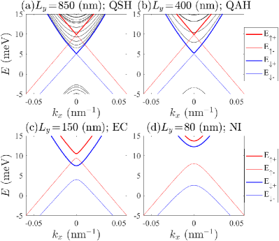
Figure 1: (Color online) Energy bands for the Floquet Hamiltonian of the HgTe/(Hg,Cd)Te with different size $L_{y}$ under open boundary condition along the $y$ direction and periodic boundary conditions along the $x$ direction. (a) $L_{y}=850$ nm corresponds to quantum spin Hall (QSH). (b) $L_{y}=400$ nm corresponds to quantum anomalous Hall (QAH). (c) $L_{y}=150$ nm corresponds to edge conducting (EC). (d) $L_{y}=80$ nm corresponds to normal insulator (NI). Here, the definitions of $E_{\uparrow\pm}$ and $E_{\downarrow\pm}$ are the energies of two spin-up and spin-down edge bands under open boundary condition along the $y$ direction. Here, QSH is topological protected for both spin-up and spin-down edge states, QAH is topological protected for one of them only, and EC for none of them, although they still exist unless broken by disorder. The threshold of the energy gap for calculating the phase boundaries is 0.01 meV. The other parameters are given as $A_{0}=0.06$ nm^-1, $a_{x}=a_{y}=1$ nm, $\varphi=\pi/2$, and $\hbar\omega=150$ meV. Here, $a_{x}$ and $a_{y}$ are the lattice constants along the $x$ and $y$ directions, respectively. Notice that we have mapped the continuous model Hamiltonian (4) into the lattice Hamiltonian (the detailed derivations can be found in Appendix C).

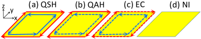
Figure 2: (Color online) Schematic diagram (or physical picture) for the four phases with the clockwise (red lines) and anticlockwise (blue lines) charge currents of the spin-up and spin-down edge states, respectively. (a) QSH state, (b) QAH state, (c) EC state, and (d) NI state. The solid red line denotes the current for the spin-up edge states, the solid blue line denotes the current for the spin-down edge states, and the dashed red and blue lines denote the currents for the spin-up and spin-down edge states possible with the disorder, respectively. It means that the dashed lines refer to states that are not protected against disorder.

In order to explore how sufficiently small system sizes can lead to Floquet phase transitions in a QSH system, we calculate the tight-binding energy spectra of a HgTe/(Hg,Cd)Te quantum well with fixed light intensity in a stripe geometry with sample width $L_{y}$ along the $y$ direction, and the system length in the $x$ direction is infinite. The energy gap opening and closing in the energy dispersions of the edge states is the most important feature of finite-size effects with fixed light intensity.

As shown in Fig. 1, we calculate the energy spectra of the HgTe/(Hg,Cd)Te with fixed light intensity $A_{0}=0.06$ nm^-1 and different width $L_{y}$ under the open boundary condition along the $y$ direction and periodic boundary conditions along the $x$ direction (the detailed derivations can be found in Appendix C). In addition, we give the detailed derivations of the tight-binding model under the open boundary condition along the $x$ direction and periodic boundary conditions along the $y$ direction in Appendix D. In Fig. 1, the red thick line indicates the upper band $E_{\uparrow+}$ of the spin-up edge states, the red thin line indicates the lower band $E_{\uparrow-}$ of the spin-up edge states, the blue thick line indicates the upper band $E_{\downarrow+}$ of the spin-down edge states, and the blue thin line indicates the lower band $E_{\downarrow-}$ of the spin-down edge states.

To illustrate the physical picture for the four phases with different system widths in Fig. 1, we provide a schematic diagram for the four phases with the clockwise (red lines) and anticlockwise (blue lines) charge currents of the spin-up and spin-down edge states, respectively, as shown in Fig. 2.

In Fig. 1(a), the system width is $L_{y}=850$ nm which is sufficiently large that there is no coupling between edge states. It is found that the energy dispersions for both spin-up and spin-down edge states are gapless and each spin state provides a charge conductance $e^{2}/h$, as shown in Fig. 2(a). This indicates that the system is in the QSH state which is time-reversal symmetry broken due to circularly polarized light; the corresponding charge conductance along the $x$ direction is $2e^{2}/h$, as shown in Fig. 2(a), with the contributions from both spin-up and spin-down charge currents flowing from higher potential to lower potential; and it is robust against the disorder.

In Fig. 1(b), the system width is decreased to $L_{y}=400$ nm, where the coupling between the spin-down edge states is strong enough to open an energy gap in the corresponding energy dispersions, while the energy dispersions of the spin-up edge states remain gapless which provides a charge conductance $e^{2}/h$. As a result, the spin-down edge states can easily be broken by the disorder. This is because the transport electrons in the spin-down edge channels can possibly be backscattered by impurities. Hence, the charge conductance along the $x$ direction in this state ranges from $e^{2}/h$ to $2e^{2}/h$ with disorder, as shown in Fig. 2(b). This state is called the QAH state Fu et al. (2014).

In Fig. 1(c), when the system width decreases to $L_{y}=150$ nm, all the energy dispersions of the edge states become gapped. Particularly, the lower band of the spin-up edge states is higher than the upper band of the spin-down edge states near the $k_{x}=0$ point. Therefore, there are always conducting edge channels near the Fermi level which is in the bulk gap. This state is called the EC state Fu et al. (2014), in which the charge currents through the edge can be killed by disorder. So the corresponding charge conductance along the $x$ direction ranges from $0$ to $2e^{2}/h$, as shown in Fig. 2(c). In Fig. 1(d), by further decreasing the system width to $L_{y}=80$ nm, there is a bulk energy gap in the energy dispersions and we get a NI state which corresponds to Fig. 2(d) and is induced by finite-size effects.

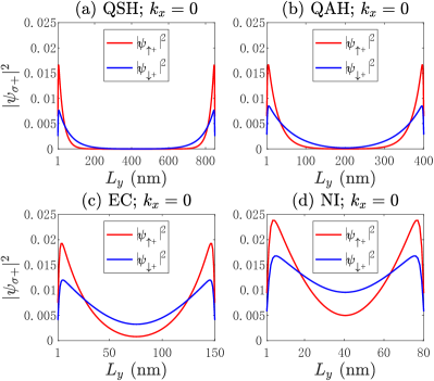
Figure 3: (Color online) Probability distributions of the edge states for the Floquet Hamiltonian of the HgTe/(Hg,Cd)Te with different size $L_{y}$ under $k_{x}=0$. The other parameters are the same as those in Fig. 1. Notice that the subscript $+$ denotes the edge states of $E_{\sigma+}$ with $\sigma=\uparrow,\downarrow$. The red solid curve denotes the probability distribution for the spin-$\uparrow$ edge state and the blue solid curve denotes the one for the spin-$\downarrow$ edge state. The density distributions of the edge states for $E_{\sigma-}$ can be found in Appendix E.

Meanwhile, along the $y$ direction, the edge states have a probability distribution in the sense of the wave function of edge states. As shown in Fig. 3, one can obtain a clear idea of how well-located edge states are forced to be mixed by changing $L_{y}$. Here, the red solid curve denotes the probability distribution for the spin-$\uparrow$ edge state and the blue solid curve denotes the one for the spin-$\downarrow$ edge state. It is indicated from Fig. 3(a) that the wave functions for both spin-$\uparrow$ and spin-$\downarrow$ edge states are well localized at the left and right edges of the system with large system width $L_{y}=850$ nm where there is no coupling between the edge states. When the system width $L_{y}$ becomes smaller and smaller, as shown in Figs. 3(b)–3(d), it is found that the edge localizations of the wave functions of the edge states get worse and worse.

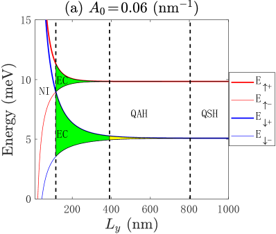
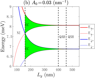
Figure 4: (Color online) Band energies $E_{\uparrow\pm}$ and $E_{\downarrow\pm}$ at the zero momentum point $k_{x}=0$ as a function of the size $L_{y}$ with fixed (a) $A_{0}=0.06$ nm^-1 and (b) $A_{0}=0.03$ nm^-1 under the open boundary condition along the $y$ direction and periodic boundary conditions along the $x$ direction. The threshold of the energy gap for calculating the phase boundaries is $0.01$ meV. The other parameters are the same as those in Fig. 1.

We furthermore investigate phase crossover due to adjusting the finite system width, with light intensity fixed. In Fig. 4, the definitions of $E_{\uparrow\pm}$ and $E_{\downarrow\pm}$ are the energies of two spin-up and spin-down edge bands at the zero momentum point $k_{x}=0$ under the open boundary condition along the $y$ direction. Meanwhile, the red thick line indicates the upper band $E_{\uparrow+}$ of the spin-up edge states, the red thin line indicates the lower band $E_{\uparrow-}$ of the spin-up edge states, the blue thick line indicates the upper band $E_{\downarrow+}$ of the spin-down edge states, and the blue thin line indicates the lower band $E_{\downarrow-}$ of the spin-down edge states.

We calculate the energies ($E_{\uparrow\pm}$ and $E_{\downarrow\pm}$) of the spin-up and spin-down edge states at $k_{x}=0$ as a function of the system width $L_{y}$ as shown in Fig. 4(a) with the same parameters as those in Fig. 1. When $L_{y}$ is very small, the energy gap for both bulk and edge states is large and the system is insulating in the NI state. By gradually increasing the width $L_{y}$, once the lower energy band of the spin-up edge states touches the upper energy band of the spin-down edge states, the system enters into the EC state. Particularly, we notice that there is a critical point which separates the EC state from the NI state, as shown in Fig. 4. In the EC state, the lower energy band of the spin-up edge states is higher than the upper energy band of the spin-down edge states, and the energy dispersions for both spin-up and spin-down edge states are gapped. By further increasing the width $L_{y}$, the energy gap of the spin-up edge states vanishes but the energy dispersion for the spin-down edge states is still gapped. At this time, the system enters into a QAH state. When $L_{y}$ is very large, the system enters into a QSH state, where the energy dispersions for both spin-up and spin-down edge states are gapless.

Different phases are determined by the edge states and energy gaps. Here, we consider the finite-size effect on the edge states and energy gaps. However, the Chern number and Bott index are used to describe the topological properties of an infinite-size system under periodic boundary conditions both along the $x$ and $y$ directions. Therefore, for a small-size system under open boundary condition along the $y$ direction here, both the Chern number and Bott index are inapplicable. Concretely, when the system size is very small, the coupling between the edge states becomes very strong and the edge states are destroyed by opening a gap, as shown in Fig. 3(d). In addition, Ref. Zhou et al. (2008) also mentioned that the finite-size effect can destroy the quantum spin Hall effect phase without a topological index transition. Next, we will reply to the applicability of our approach to the phase transition regime. For finite small sizes, our phase transitions belong to continuous phase transitions which are in general crossovers, and we can only use the energy gaps of the edge states to determine the phase transitions quantitatively. Meanwhile, as mentioned in Ref. Fu et al. (2014), another applicable method is to calculate the transport or conductance of the finite-size system by using the Landauer-Büttiker formalism Landauer (1970); Büttiker (1988). For example, Ref. Li et al. (2011) has calculated the transport properties of a finite-size system in HgTe/CdTe quantum wells without optical pumping. We will investigate the transport properties of a finite-size Floquet system in the future.

V Overall phase diagram

In this section, we will investigate the overall phase diagram of the system.

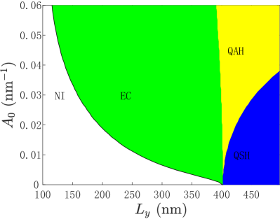
Figure 5: (Color online) Phase diagram in the system width vs. light intensity ($L_{y}$, $A_{0}$) plane under the open boundary condition along the $y$ direction and periodic boundary conditions along the $x$ direction, as determined by the long-$x$-wavelength (small-$k_{x}$) limit. There are four kinds of phase regimes, i.e., NI, EC, QAH, and QSH are shown. The white zone denotes the NI regime, the green zone denotes the EC regime, the yellow zone denotes the QAH regime, and the blue zone denotes the QAH regime. The threshold of the energy gap for calculating the phase boundaries is $0.01$ meV, which is also used as a criterion of the energy gap opening. The other parameters are the same as those in Fig. 1.

Based on the energy gap for spin-up and spin-down edge states, we plot the whole phase diagram with two tunable parameters: light intensity $A_{0}$ and system width $L_{y}$ as shown in Fig. 5. There are four kinds of phase regimes, i.e., NI, EC, QAH, and QSH, as shown in Fig. 5. An important feature is that each transport regime has its own permitted width range with fixed light intensity. For example, the width for the EC state is in the range from $116$ to $391$ nm with fixed $A_{0}=0.06$ nm^-1. The permitted width range for different transport states is important because it can help us to find the desired transport regime by choosing an appropriate device width and intensity of light.

VI Summary

Even though Floquet engineering had been extensively used to engineer various topological phases that are elusive in the static regime, our proposal instead engineers QAH and other phases in a realistic QSH setup that takes into account the hybridization effects due to the finite size of the realistic samples. We numerically investigate the light-induced topological phases and finite-size topological phase crossovers in a QSH system with high-frequency pumping optics, taking the HgTe quantum well as the paradigmatic realistic model. We find that the coupling of edge states depends on both the system width and the light intensity. Furthermore, we can get four different topological transport regimes by choosing the proper width and light intensity. Since the intensity of light can easily be continuously tuned in experiments, our proposal that uses circularly polarized light instead of magnetic doping provides a feasible route towards realizing QAH states in experiments.

With state-of-the-art nanofabrication, it is possible to engineer realistic quantum materials to reduce its size in the length scale presented in our figures. For example, in Ref. Qiu et al. (2022), it is reported that the quantum anomalous Hall (QAH) devices can be fabricated as miniaturized with channel widths down to 600 nm in six quintuple layers of Cr_0.12(Bi_0.26Sb_0.62)₂Te₃ film which were epitaxially deposited onto GaAs (111) substrates. Furthermore, they measured the longitudinal and transverse resistivities in four devices with a channel width of 0.6, 1.5, 3, and 5 $\mu$m Qiu et al. (2022). Meanwhile, Ref. Zhou et al. (2022) demonstrates that the QAH effect persists in a Hall bar device with width 72 nm in three quintuple layers of Cr-doped (Bi,Sb)₂Te₃, four quintuple layers of (Bi,Sb)₂Te₃, and three quintuple layers of Cr-doped (Bi,Sb)₂Te₃ Zhao et al. (2020, 2022), and they measured the transverse resistance and longitudinal resistance in Hall bar devices with widths from 300 nm to 10 $\mu$m. Technologically, first, by using photolithography, the samples can be patterned into a Hall bar with width 10 $\mu$m Qiu et al. (2022); Zhou et al. (2022). Then by using another experimental technology, i.e., electron-beam lithography, the realization of the QAH bar devices with widths from 10 $\mu$m down to 72 nm are further fabricated Zhou et al. (2022).

Appendix A Expressions for ${\cal H}_{0,0}$, ${\cal H}_{0,-1}$, and ${\cal H}_{0,1}$

The motivation for Appendix A is to show the concrete analytical expressions for ${\cal H}_{0,0}$, ${\cal H}_{0,-1}$, and ${\cal H}_{0,1}$ in the Floquet Hamiltonian (3) of the main text. The concrete analytical expressions for ${\cal H}_{0,0}$, ${\cal H}_{0,-1}$, and ${\cal H}_{0,1}$ in the Floquet Hamiltonian (3) are given as

$${\cal H}_{0,0} \!=\![C-D(A_{0}^{2}+k_{x}^{2}+k_{y}^{2})]\tau_{0}\otimes\sigma_{0}+Ak_{x}\tau_{z}\otimes\sigma_{x}+[M-B(A_{0}^{2}+k_{x}^{2}+k_{y}^{2})]\tau_{0}\otimes\sigma_{z}+Ak_{y}\tau_{0}\otimes\sigma_{y}$$

$$\!=\!{\cal H}({\bf k})-DA_{0}^{2}\tau_{0}\otimes\sigma_{0}-BA_{0}^{2}\tau_{0}\otimes\sigma_{z},$$ (7)

$$\!{\cal H}_{0,-1} \!=\!iDA_{0}(k_{x}\!+\!e^{-i\varphi}k_{y})\tau_{0}\otimes\sigma_{0}\!+\!iBA_{0}(k_{x}\!+\!e^{-i\varphi}k_{y})\tau_{0}\otimes\sigma_{z}\!-\!\frac{i}{2}AA_{0}\tau_{z}\otimes\sigma_{x}\!-\!\frac{i}{2}AA_{0}e^{-i\varphi}\tau_{0}\otimes\sigma_{y},$$ (8)

$$\!{\cal H}_{0,1} \!=\!\!-\!iDA_{0}(k_{x}\!+\!e^{i\varphi}k_{y})\tau_{0}\otimes\sigma_{0}\!-\!iBA_{0}(k_{x}\!+\!e^{i\varphi}k_{y})\tau_{0}\otimes\sigma_{z}\!+\!\frac{i}{2}AA_{0}\tau_{z}\otimes\sigma_{x}\!+\!\frac{i}{2}AA_{0}e^{i\varphi}\tau_{0}\otimes\sigma_{y}.$$ (9)

Appendix B Time-reversal symmetry

The motivation for Appendix B is to prove that when $\varphi=0$, the Floquet Hamiltonian (4) in the main text still satisfies the time-reversal symmetry. However, when $\varphi\neq 0$, the time-reversal symmetry of the Hamiltonian (4) is broken.

The Floquet Hamiltonian (4) under time-reversal transformation becomes

$$~{}~{}{\cal T}{\cal H}^{(F)}({\bf k}){\cal T}^{-1}$$

$$\!=\!i\tau_{y}\otimes\sigma_{0}{\cal K}\left[-D(A_{0}^{2}+k^{2})\tau_{0}\otimes\sigma_{0}+A(k_{x}\tau_{z}\otimes\sigma_{x}+k_{y}\tau_{0}\otimes\sigma_{y})+(\!M\!-\!BA_{0}^{2}\!-\!Bk^{2})\tau_{0}\otimes\sigma_{z}\right]{\cal K}^{-1}(i\tau_{y}\otimes\sigma_{0})^{-1}$$

$$\!-\!\frac{A_{0}^{2}\sin\varphi}{\hbar\omega}i\tau_{y}\otimes\sigma_{0}{\cal K}\left[2AB(k_{x}\tau_{0}\otimes\sigma_{x}+k_{y}\tau_{z}\otimes\sigma_{y})+A^{2}\tau_{z}\otimes\sigma_{z}\right]{\cal K}^{-1}(i\tau_{y}\otimes\sigma_{0})^{-1}$$

$$\!=\!-D(A_{0}^{2}+k^{2})\tau_{0}\otimes\sigma_{0}-A(k_{x}\tau_{z}\otimes\sigma_{x}+k_{y}\tau_{0}\otimes\sigma_{y})+(\!M\!-\!BA_{0}^{2}\!-\!Bk^{2})\tau_{0}\otimes\sigma_{z}$$

$$\!-\!\frac{A_{0}^{2}\sin\varphi}{\hbar\omega}\left[2AB(k_{x}\tau_{0}\otimes\sigma_{x}+k_{y}\tau_{z}\otimes\sigma_{y})-A^{2}\tau_{z}\otimes\sigma_{z}\right]$$

$$\!=\!{\cal H}^{(F)}(-{\bf k})\!-\!\frac{2A_{0}^{2}\sin\varphi}{\hbar\omega}\left[2AB(k_{x}\tau_{0}\otimes\sigma_{x}+k_{y}\tau_{z}\otimes\sigma_{y})-A^{2}\tau_{z}\otimes\sigma_{z}\right],$$ (10)

where ${\cal T}=i\tau_{y}\otimes\sigma_{0}{\cal K}$ Michetti et al. (2012) is the time-reversal operator with the complex conjugate operator ${\cal K}$, we have ${\cal K}{\cal H}^{(F)}({\bf k}){\cal K}^{-1}={\cal H}^{(F)*}({\bf k})$, and we use

$$(i\tau_{y}\otimes\sigma_{0})(\tau_{0}\otimes\sigma_{0})(i\tau_{y}\otimes\sigma_{0})^{-1}=\tau_{0}\otimes\sigma_{0},$$ (11)

$$(i\tau_{y}\otimes\sigma_{0})(\tau_{z}\otimes\sigma_{x})(i\tau_{y}\otimes\sigma_{0})^{-1}=-\tau_{z}\otimes\sigma_{x},$$ (12)

$$(i\tau_{y}\otimes\sigma_{0})(K\tau_{0}\otimes\sigma_{y}K^{-1})(i\tau_{y}\otimes\sigma_{0})^{-1}=-\tau_{0}\otimes\sigma_{y},$$ (13)

$$(i\tau_{y}\otimes\sigma_{0})(\tau_{0}\otimes\sigma_{z})(i\tau_{y}\otimes\sigma_{0})^{-1}=\tau_{0}\otimes\sigma_{z},$$ (14)

$$(i\tau_{y}\otimes\sigma_{0})(\tau_{0}\otimes\sigma_{x})(i\tau_{y}\otimes\sigma_{0})^{-1}=\tau_{0}\otimes\sigma_{x},$$ (15)

$$(i\tau_{y}\otimes\sigma_{0})(K\tau_{z}\otimes\sigma_{y}K^{-1})(i\tau_{y}\otimes\sigma_{0})^{-1}=\tau_{z}\otimes\sigma_{y},$$ (16)

$$(i\tau_{y}\otimes\sigma_{0})(\tau_{z}\otimes\sigma_{z})(i\tau_{y}\otimes\sigma_{0})^{-1}=-\tau_{z}\otimes\sigma_{z}.$$ (17)

As a result of Eq. (B), if $\varphi=0$, we have ${\cal T}{\cal H}^{(F)}({\bf k}){\cal T}^{-1}={\cal H}^{(F)}(-{\bf k})$ which shows a time-reversal symmetry. However, for $\varphi\neq 0$, Eq. (B) shows that the time-reversal symmetry is broken.

Appendix C Tight-binding model under the open boundary condition along the $y$ direction and periodic boundary conditions along the $x$ direction

The motivation of Appendix C is to derive the analytical expression of the tight-binding model Hamiltonian under the open boundary condition along the $y$ direction and periodic boundary conditions along the $x$ direction for the further numerical calculations in the main text.

In a lattice, one makes the following replacements Shen (2012):

$$k_{j}\rightarrow\frac{1}{a_{j}}\sin(k_{j}a_{j}),$$ (18)

$$k_{j}^{2}\rightarrow\frac{2}{a_{j}^{2}}[1-\cos(k_{j}a_{j})],$$ (19)

where $j=x,y,z$, $a_{j}$ is the lattice constant along the $j$ direction, $\sin(k_{j}a_{j})=\frac{e^{ik_{j}a_{j}}-e^{-ik_{j}a_{j}}}{2i}$, and $\cos(k_{j}a_{j})=\frac{e^{ik_{j}a_{j}}+e^{-ik_{j}a_{j}}}{2}$,

$$k^{2}\rightarrow\frac{2}{a_{x}^{2}}[1-\cos(k_{x}a_{x})]+\frac{2}{a_{y}^{2}}[1-\cos(k_{y}a_{y})],$$ (20)

where $k^{2}=k_{x}^{2}+k_{y}^{2}$. In this way, the hopping terms in the lattice model only exist between the nearest-neighbor sites. With this mapping, one obtains the following tight-binding model with high-frequency pumping in the basis $(c_{{\bf k},+,\uparrow},c_{{\bf k},-,\uparrow},c_{{\bf k},+,\downarrow},c_{{\bf k},-,\downarrow})^{T}$ as

$$\!{\cal H}^{(F)}({\bf k})\!=\!\left(\begin{array}[]{cccc}h_{\uparrow}({\bf k})&0\\ 0&h_{\downarrow}({\bf k})\end{array}\right),$$ (23)

where

$$h_{\uparrow}({\bf k}) \!=\!\!-\!D\left\{A_{0}^{2}\!+\!\frac{2}{a_{x}^{2}}[1\!-\!\cos(k_{x}a_{x})]\!+\!\frac{2}{a_{y}^{2}}[1\!-\!\cos(k_{y}a_{y})]\right\}\sigma_{0}$$

$$\!+\!\left\{M\!-\!B\left[A_{0}^{2}\!+\!\frac{2}{a_{x}^{2}}[1\!-\!\cos(k_{x}a_{x})]\!+\!\frac{2}{a_{y}^{2}}[1\!-\!\cos(k_{y}a_{y})]\right]\!-\!\frac{A_{0}^{2}A^{2}\sin\varphi}{\hbar\omega}\right\}\sigma_{z}$$

$$\!+\!\left(\!1\!-\!\frac{2A_{0}^{2}B\sin\varphi}{\hbar\omega}\!\right)A\left[\frac{1}{a_{x}}\sin(k_{x}a_{x})\!-\!\frac{i}{a_{y}}\sin(k_{y}a_{y})\right]\sigma_{+}$$

$$\!+\!\left(\!1\!-\!\frac{2A_{0}^{2}B\sin\varphi}{\hbar\omega}\!\right)A\left[\frac{1}{a_{x}}\sin(k_{x}a_{x})\!+\!\frac{i}{a_{y}}\sin(k_{y}a_{y})\right]\sigma_{-},$$ (24)

$$h_{\downarrow}({\bf k}) \!=\!\!-\!D\left\{A_{0}^{2}\!+\!\frac{2}{a_{x}^{2}}[1\!-\!\cos(k_{x}a_{x})]\!+\!\frac{2}{a_{y}^{2}}[1\!-\!\cos(k_{y}a_{y})]\right\}\sigma_{0}$$

$$\!+\!\left\{M\!-\!B\left[A_{0}^{2}\!+\!\frac{2}{a_{x}^{2}}[1\!-\!\cos(k_{x}a_{x})]\!+\!\frac{2}{a_{y}^{2}}[1\!-\!\cos(k_{y}a_{y})]\right]\!+\!\frac{A_{0}^{2}A^{2}\sin\varphi}{\hbar\omega}\right\}\sigma_{z}$$

$$\!-\!\left(\!1\!+\!\frac{2A_{0}^{2}B\sin\varphi}{\hbar\omega}\!\right)A\left[\frac{1}{a_{x}}\sin(k_{x}a_{x})\!+\!\frac{i}{a_{y}}\sin(k_{y}a_{y})\right]\sigma_{+}$$

$$\!-\!\left(\!1\!+\!\frac{2A_{0}^{2}B\sin\varphi}{\hbar\omega}\!\right)A\left[\frac{1}{a_{x}}\sin(k_{x}a_{x})\!-\!\frac{i}{a_{y}}\sin(k_{y}a_{y})\right]\sigma_{-}.$$ (25)

Performing the Fourier transformation, one obtains

$$c_{{\bf k},s,\sigma} =\frac{1}{\sqrt{N_{y}}}\sum_{k_{x},j_{y}}^{N_{y}}e^{-ik_{y}j_{y}a_{y}}c_{k_{x},j_{y},s,\sigma},$$ (26)

$$c_{{\bf k},s,\sigma}^{\dagger} =\frac{1}{\sqrt{N_{y}}}\sum_{k_{x},j_{y}}^{N_{y}}e^{ik_{y}j_{y}a_{y}}c_{k_{x},j_{y},s,\sigma}^{\dagger}.$$ (27)

$$C_{{\bf k},\sigma} =\begin{pmatrix}c_{{\bf k},+,\sigma}\\ c_{{\bf k},-,\sigma}\end{pmatrix}=\frac{1}{\sqrt{N_{y}}}\sum_{k_{x},j_{y}}^{N_{y}}e^{-ik_{y}j_{y}a_{y}}C_{k_{x},j_{y},\sigma},$$ (28)

$$C_{{\bf k},\sigma}^{\dagger} =\begin{pmatrix}c_{{\bf k},+,\sigma}^{\dagger}&c_{{\bf k},-,\sigma}^{\dagger}\end{pmatrix}=\frac{1}{\sqrt{N_{y}}}\sum_{k_{x},j_{y}}^{N_{y}}e^{ik_{y}j_{y}a_{y}}C_{k_{x},j_{y},\sigma}^{\dagger}.$$ (29)

$$~{}~{}\sum_{{\bf k},s}C_{{\bf k},\uparrow}^{\dagger}\left[h_{\uparrow}({\bf k})\right]C_{{\bf k},\uparrow}$$

$$\!=\!\!-\!D\sum_{k_{x},j_{y}}\!\left[\!A_{0}^{2}\!+\!\frac{2}{a_{x}^{2}}\!+\!\frac{2}{a_{y}^{2}}\!-\!\frac{2}{a_{x}^{2}}\cos(k_{x}a_{x})\!\right]\!C_{k_{x},j_{y},\uparrow}^{\dagger}\sigma_{0}C_{k_{x},j_{y},\uparrow}\!+\!\frac{D}{a_{y}^{2}}\sum_{k_{x},j_{y}}\!\left[\!C_{k_{x},j_{y},\uparrow}^{\dagger}\sigma_{0}C_{k_{x},j_{y}+1,\uparrow}\!+\!{\rm h.c.}\!\right]\!$$

$$\!+\!\sum_{k_{x},j_{y}}\!\left[\!M\!-\!BA_{0}^{2}\!-\!\frac{2B}{a_{x}^{2}}\!-\!\frac{2B}{a_{y}^{2}}\!+\!\frac{2B}{a_{x}^{2}}\cos(k_{x}a_{x})\!-\!\frac{A_{0}^{2}A^{2}\sin\varphi}{\hbar\omega}\!\right]\!C_{k_{x},j_{y},\uparrow}^{\dagger}\sigma_{z}C_{k_{x},j_{y},\uparrow}\!+\!\frac{B}{a_{y}^{2}}\sum_{k_{x},j_{y}}\!\left[\!C_{k_{x},j_{y},\uparrow}^{\dagger}\!\sigma_{z}\!C_{k_{x},j_{y}+1,\uparrow}\!+\!{\rm h.c.}\!\right]\!$$

$$\!+\!\left(\!1\!-\!\frac{2A_{0}^{2}B\sin\varphi}{\hbar\omega}\!\right)\frac{A}{a_{x}}\sum_{k_{x},j_{y}}\sin(k_{x}a_{x})\!\left[\!C_{k_{x},j_{y},\uparrow}^{\dagger}(\sigma_{+}+\sigma_{-})C_{k_{x},j_{y},\uparrow}\!\right]\!$$

$$\!+\!\left(\!1\!-\!\frac{2A_{0}^{2}B\sin\varphi}{\hbar\omega}\!\right)\frac{A}{2a_{y}}\sum_{k_{x},j_{y}}\!\left[\!C_{k_{x},j_{y},\uparrow}^{\dagger}(\sigma_{-}-\sigma_{+})C_{k_{x},j_{y}+1,\uparrow}\!+\!C_{k_{x},j_{y}+1,\uparrow}^{\dagger}(\sigma_{+}-\sigma_{-})C_{k_{x},j_{y},\uparrow}\!\right],$$ (30)

where

$$C_{k_{x},j_{y},\uparrow}^{\dagger}(\sigma_{-}-\sigma_{+})C_{k_{x},j_{y}+1,\uparrow}$$

$$=\begin{pmatrix}c_{k_{x},+,j_{y},\uparrow}^{\dagger}&c_{k_{x},-,j_{y},\uparrow}^{\dagger}\end{pmatrix}\begin{pmatrix}0&-1\\ 1&0\end{pmatrix}\begin{pmatrix}c_{k_{x},+,j_{y}+1,\uparrow}\\ c_{k_{x},-,j_{y}+1,\uparrow}\end{pmatrix}=\begin{pmatrix}c_{k_{x},-,j_{y},\uparrow}^{\dagger}&-c_{k_{x},+,j_{y},\uparrow}^{\dagger}\end{pmatrix}\begin{pmatrix}c_{k_{x},+,j_{y}+1,\uparrow}\\ c_{k_{x},-,j_{y}+1,\uparrow}\end{pmatrix}$$

$$=c_{k_{x},-,j_{y},\uparrow}^{\dagger}c_{k_{x},+,j_{y}+1,\uparrow}-c_{k_{x},+,j_{y},\uparrow}^{\dagger}c_{k_{x},-,j_{y}+1,\uparrow},$$ (31)

$$C_{k_{x},j_{y},\uparrow}^{\dagger}(\sigma_{+}-\sigma_{-})C_{k_{x},j_{y}+1,\uparrow}$$

$$=\begin{pmatrix}c_{k_{x},+,j_{y},\uparrow}^{\dagger}&c_{k_{x},-,j_{y},\uparrow}^{\dagger}\end{pmatrix}\begin{pmatrix}0&1\\ -1&0\end{pmatrix}\begin{pmatrix}c_{k_{x},+,j_{y}+1,\uparrow}\\ c_{k_{x},-,j_{y}+1,\uparrow}\end{pmatrix}=\begin{pmatrix}-c_{k_{x},-,j_{y},\uparrow}^{\dagger}&c_{k_{x},+,j_{y},\uparrow}^{\dagger}\end{pmatrix}\begin{pmatrix}c_{k_{x},+,j_{y}+1,\uparrow}\\ c_{k_{x},-,j_{y}+1,\uparrow}\end{pmatrix}$$

$$=-c_{k_{x},-,j_{y},\uparrow}^{\dagger}c_{k_{x},+,j_{y}+1,\uparrow}+c_{k_{x},+,j_{y},\uparrow}^{\dagger}c_{k_{x},-,j_{y}+1,\uparrow}=c_{k_{x},+,j_{y},\uparrow}^{\dagger}c_{k_{x},-,j_{y}+1,\uparrow}-c_{k_{x},-,j_{y},\uparrow}^{\dagger}c_{k_{x},+,j_{y}+1,\uparrow}$$

$$=(c_{k_{x},-,j_{y},\uparrow}^{\dagger}c_{k_{x},+,j_{y}+1,\uparrow}-c_{k_{x},+,j_{y},\uparrow}^{\dagger}c_{k_{x},-,j_{y}+1,\uparrow})^{\dagger}.$$ (32)

Therefore, we have

$$~{}~{}\sum_{{\bf k},s}C_{{\bf k},\uparrow}^{\dagger}\left[h_{\uparrow}({\bf k})\right]C_{{\bf k},\uparrow}$$

$$\!=\!\!-\!D\sum_{k_{x},j_{y}}\!\left[\!A_{0}^{2}\!+\!\frac{2}{a_{x}^{2}}\!+\!\frac{2}{a_{y}^{2}}\!-\!\frac{2}{a_{x}^{2}}\cos(k_{x}a_{x})\!\right]\!C_{k_{x},j_{y},\uparrow}^{\dagger}\sigma_{0}C_{k_{x},j_{y},\uparrow}\!+\!\frac{D}{a_{y}^{2}}\sum_{k_{x},j_{y}}\!\left[\!C_{k_{x},j_{y},\uparrow}^{\dagger}\sigma_{0}C_{k_{x},j_{y}+1,\uparrow}\!+\!{\rm h.c.}\!\right]\!$$

$$\!+\!\sum_{k_{x},j_{y}}\!\left[\!M\!-\!BA_{0}^{2}\!-\!\frac{2B}{a_{x}^{2}}\!-\!\frac{2B}{a_{y}^{2}}\!+\!\frac{2B}{a_{x}^{2}}\cos(k_{x}a_{x})\!-\!\frac{A_{0}^{2}A^{2}\sin\varphi}{\hbar\omega}\!\right]\!C_{k_{x},j_{y},\uparrow}^{\dagger}\sigma_{z}C_{k_{x},j_{y},\uparrow}\!+\!\frac{B}{a_{y}^{2}}\sum_{k_{x},j_{y}}\!\left[\!C_{k_{x},j_{y},\uparrow}^{\dagger}\!\sigma_{z}\!C_{k_{x},j_{y}+1,\uparrow}\!+\!{\rm h.c.}\!\right]\!$$

$$\!+\!\left(\!1\!-\!\frac{2A_{0}^{2}B\sin\varphi}{\hbar\omega}\!\right)\frac{A}{a_{x}}\sum_{k_{x},j_{y}}\sin(k_{x}a_{x})\!\left[\!C_{k_{x},j_{y},\uparrow}^{\dagger}(\sigma_{+}+\sigma_{-})C_{k_{x},j_{y},\uparrow}\!\right]\!$$

$$\!+\!\left(\!1\!-\!\frac{2A_{0}^{2}B\sin\varphi}{\hbar\omega}\!\right)\frac{A}{2a_{y}}\sum_{k_{x},j_{y}}\!\left[\!C_{k_{x},j_{y},\uparrow}^{\dagger}(\sigma_{-}-\sigma_{+})C_{k_{x},j_{y}+1,\uparrow}\!+\!{\rm h.c.}\!\right].$$ (33)

$$~{}~{}\sum_{{\bf k},s}C_{{\bf k},\downarrow}^{\dagger}\left[h_{\downarrow}({\bf k})\right]C_{{\bf k},\downarrow}$$

$$\!=\!\!-\!D\sum_{k_{x},j_{y}}\!\left[\!A_{0}^{2}\!+\!\frac{2}{a_{x}^{2}}\!+\!\frac{2}{a_{y}^{2}}\!-\!\frac{2}{a_{x}^{2}}\cos(k_{x}a_{x})\!\right]\!C_{k_{x},j_{y},\uparrow}^{\dagger}\sigma_{0}C_{k_{x},j_{y},\uparrow}\!+\!\frac{D}{a_{y}^{2}}\sum_{k_{x},j_{y}}\!\left[\!C_{k_{x},j_{y},\uparrow}^{\dagger}\sigma_{0}C_{k_{x},j_{y}+1,\uparrow}\!+\!{\rm h.c.}\!\right]\!$$

$$\!+\!\sum_{k_{x},j_{y}}\!\left[\!M\!-\!BA_{0}^{2}\!-\!\frac{2B}{a_{x}^{2}}\!-\!\frac{2B}{a_{y}^{2}}\!+\!\frac{2B}{a_{x}^{2}}\cos(k_{x}a_{x})\!+\!\frac{A_{0}^{2}A^{2}\sin\varphi}{\hbar\omega}\!\right]\!C_{k_{x},j_{y},\uparrow}^{\dagger}\sigma_{z}C_{k_{x},j_{y},\uparrow}\!+\!\frac{B}{a_{y}^{2}}\sum_{k_{x},j_{y}}\!\left[\!C_{k_{x},j_{y},\uparrow}^{\dagger}\!\sigma_{z}\!C_{k_{x},j_{y}+1,\uparrow}\!+\!{\rm h.c.}\!\right]\!$$

$$\!-\!\left(\!1\!+\!\frac{2A_{0}^{2}B\sin\varphi}{\hbar\omega}\!\right)\frac{A}{a_{x}}\sum_{k_{x},j_{y}}\sin(k_{x}a_{x})\!\left[\!C_{k_{x},j_{y},\uparrow}^{\dagger}(\sigma_{+}+\sigma_{-})C_{k_{x},j_{y},\uparrow}\!\right]\!$$

$$\!-\!\left(\!1\!+\!\frac{2A_{0}^{2}B\sin\varphi}{\hbar\omega}\!\right)\frac{A}{2a_{y}}\sum_{k_{x},j_{y}}\!\left[\!C_{k_{x},j_{y},\uparrow}^{\dagger}(\sigma_{+}-\sigma_{-})C_{k_{x},j_{y}+1,\uparrow}\!+\!{\rm h.c.}\!\right].$$ (34)

Therefore, the tight-binding Hamiltonian under $x$ periodic boundary conditions (PBCs) and $y$ open boundary conditions (OBCs) in the basis $(C_{k_{x},1,\uparrow},C_{k_{x},1,\downarrow},C_{k_{x},2,\uparrow},C_{k_{x},2,\downarrow},\cdots,C_{k_{x},N_{y},\uparrow},C_{k_{x},N_{y},\downarrow})^{T}$ is given by

$${\cal H}_{y-OBC}^{(F)}(k_{x})=\begin{pmatrix}h&T&0&\cdots&0\\ T^{\dagger}&h&T&\cdots&0\\ 0&T^{\dagger}&h&\ddots&\vdots\\ \vdots&\ddots&\ddots&\ddots&T\\ 0&\cdots&0&T^{\dagger}&h\end{pmatrix}_{(4N_{y})\times(4N_{y})},$$ (35)

where

$$h\!=\!\begin{pmatrix}\!h_{\uparrow}&0\\ 0&h_{\downarrow}\!\end{pmatrix},$$ (36)

$$h_{\uparrow}\!=\!E_{0}\sigma_{0}\!+\!\Delta_{\uparrow}\sigma_{z}\!+\!\Gamma_{\uparrow}(\!\sigma_{+}\!+\!\sigma_{-}\!)\!=\!E_{0}\sigma_{0}\!+\!\Delta_{\uparrow}\sigma_{z}\!+\!\Gamma_{\uparrow}\sigma_{x},~{}~{}h_{\downarrow}\!=\!E_{0}\sigma_{0}\!+\!\Delta_{\downarrow}\sigma_{z}\!+\!\Gamma_{\downarrow}(\!\sigma_{+}\!+\!\sigma_{-}\!)\!=\!E_{0}\sigma_{0}\!+\!\Delta_{\downarrow}\sigma_{z}\!+\!\Gamma_{\downarrow}\sigma_{x},$$ (37)

$$E_{0}\!=\!-\!D\!\left[\!A_{0}^{2}\!+\!\frac{2}{a_{x}^{2}}\!+\!\frac{2}{a_{y}^{2}}\!-\!\frac{2}{a_{x}^{2}}\cos(k_{x}a_{x})\!\right]\!=\!-DA_{0}^{2}\!-\!\frac{2D}{a_{x}^{2}}\!-\!\frac{2D}{a_{y}^{2}}\!+\!\frac{2D}{a_{x}^{2}}\cos(k_{x}a_{x}),$$ (38)

$$\Delta_{\uparrow}\!=\!M\!-\!BA_{0}^{2}\!-\!\frac{2B}{a_{x}^{2}}\!-\!\frac{2B}{a_{y}^{2}}\!+\!\frac{2B}{a_{x}^{2}}\cos(k_{x}a_{x})\!-\!\frac{A_{0}^{2}A^{2}\sin\varphi}{\hbar\omega},~{}~{}\Delta_{\downarrow}\!=\!M\!-\!BA_{0}^{2}\!-\!\frac{2B}{a_{x}^{2}}\!-\!\frac{2B}{a_{y}^{2}}\!+\!\frac{2B}{a_{x}^{2}}\cos(k_{x}a_{x})\!+\!\frac{A_{0}^{2}A^{2}\sin\varphi}{\hbar\omega},$$ (39)

$$\Gamma_{\uparrow}\!=\!\left(\!1\!-\!\frac{2A_{0}^{2}B\sin\varphi}{\hbar\omega}\!\right)\frac{A}{a_{x}}\sin(k_{x}a_{x}),~{}~{}\Gamma_{\downarrow}\!=\!-\left(\!1\!+\!\frac{2A_{0}^{2}B\sin\varphi}{\hbar\omega}\!\right)\frac{A}{a_{x}}\sin(k_{x}a_{x}),$$ (40)

$$T\!=\!\begin{pmatrix}\!T_{\uparrow}&0\\ 0&T_{\downarrow}\!\end{pmatrix}\!,~{}~{}T^{\dagger}\!=\!\begin{pmatrix}\!T_{\uparrow}^{\dagger}&0\\ 0&T_{\downarrow}^{\dagger}\!\end{pmatrix}\!,$$ (41)

$$T_{\uparrow}\!=\!\frac{D}{a_{y}^{2}}\sigma_{0}\!+\!\frac{B}{a_{y}^{2}}\sigma_{z}\!+\!\left(\!1\!-\!\frac{2A_{0}^{2}B\sin\varphi}{\hbar\omega}\!\right)\frac{A}{2a_{y}}(\sigma_{-}-\sigma_{+}),~{}~{}T^{\dagger}_{\uparrow}\!=\!\frac{D}{a_{y}^{2}}\sigma_{0}\!+\!\frac{B}{a_{y}^{2}}\sigma_{z}\!+\!\left(\!1\!-\!\frac{2A_{0}^{2}B\sin\varphi}{\hbar\omega}\!\right)\frac{A}{2a_{y}}(\sigma_{+}-\sigma_{-}),$$ (42)

$$T_{\downarrow}\!=\!\frac{D}{a_{y}^{2}}\sigma_{0}\!+\!\frac{B}{a_{y}^{2}}\sigma_{z}\!-\!\left(\!1\!+\!\frac{2A_{0}^{2}B\sin\varphi}{\hbar\omega}\!\right)\frac{A}{2a_{y}}(\sigma_{-}-\sigma_{+}),~{}~{}T^{\dagger}_{\downarrow}\!=\!\frac{D}{a_{y}^{2}}\sigma_{0}\!+\!\frac{B}{a_{y}^{2}}\sigma_{z}\!-\!\left(\!1\!+\!\frac{2A_{0}^{2}B\sin\varphi}{\hbar\omega}\!\right)\frac{A}{2a_{y}}(\sigma_{+}-\sigma_{-}),$$ (43)

where we use $\sigma_{+}\!+\!\sigma_{-}=\sigma_{x}$, and $\sigma_{\pm}=(\sigma_{x}\pm i\sigma_{y})/2$ are the spin-raising and spin-lowering operators, i.e.,

$$\sigma_{+}\!=\!\begin{pmatrix}0&1\\ 0&0\end{pmatrix},~{}~{}\sigma_{-}\!=\!\begin{pmatrix}0&0\\ 1&0\end{pmatrix}.$$ (44)

In addition, we can also get the tight-binding Hamiltonian with pseudo-spin-$\uparrow$ under $x$-PBCs and $y$-OBCs in the basis $(C_{k_{x},1,\uparrow},C_{k_{x},2,\uparrow},\cdots,C_{k_{x},N_{y},\uparrow})^{T}$ as

$${\cal H}_{y-OBC}^{(F)\uparrow}(k_{x})=\begin{pmatrix}h_{\uparrow}&T_{\uparrow}&0&\cdots&0\\ T_{\uparrow}^{\dagger}&h_{\uparrow}&T_{\uparrow}&\cdots&0\\ 0&T_{\uparrow}^{\dagger}&h_{\uparrow}&\ddots&\vdots\\ \vdots&\ddots&\ddots&\ddots&T_{\uparrow}\\ 0&\cdots&0&T_{\uparrow}^{\dagger}&h_{\uparrow}\end{pmatrix}_{(2N_{y})\times(2N_{y})},$$ (45)

where

$$h_{\uparrow}\!=\!E_{0}\sigma_{0}\!+\!\Delta_{\uparrow}\sigma_{z}\!+\!\Gamma_{\uparrow}(\!\sigma_{+}\!+\!\sigma_{-}\!)\!=\!E_{0}\sigma_{0}\!+\!\Delta_{\uparrow}\sigma_{z}\!+\!\Gamma_{\uparrow}\sigma_{x},$$ (46)

$$T_{\uparrow}\!=\!\frac{D}{a_{y}^{2}}\sigma_{0}\!+\!\frac{B}{a_{y}^{2}}\sigma_{z}\!+\!\left(\!1\!-\!\frac{2A_{0}^{2}B\sin\varphi}{\hbar\omega}\!\right)\frac{A}{2a_{y}}(\sigma_{-}-\sigma_{+}),~{}~{}T^{\dagger}_{\uparrow}\!=\!\frac{D}{a_{y}^{2}}\sigma_{0}\!+\!\frac{B}{a_{y}^{2}}\sigma_{z}\!+\!\left(\!1\!-\!\frac{2A_{0}^{2}B\sin\varphi}{\hbar\omega}\!\right)\frac{A}{2a_{y}}(\sigma_{+}-\sigma_{-}).$$ (47)

Further, we can get the tight-binding Hamiltonian with pseudo-spin-$\downarrow$ under $x$-PBCs and $y$-OBCs in the basis $(C_{k_{x},1,\downarrow},C_{k_{x},2,\downarrow},\cdots,C_{k_{x},N_{y},\downarrow})^{T}$ as

$${\cal H}_{y-OBC}^{(F)\downarrow}(k_{x})=\begin{pmatrix}h_{\downarrow}&T_{\downarrow}&0&\cdots&0\\ T_{\downarrow}^{\dagger}&h_{\downarrow}&T_{\downarrow}&\cdots&0\\ 0&T_{\downarrow}^{\dagger}&h_{\downarrow}&\ddots&\vdots\\ \vdots&\ddots&\ddots&\ddots&T_{\downarrow}\\ 0&\cdots&0&T_{\downarrow}^{\dagger}&h_{\downarrow}\end{pmatrix}_{(2N_{y})\times(2N_{y})},$$ (48)

where

$$h_{\downarrow}\!=\!E_{0}\sigma_{0}\!+\!\Delta_{\downarrow}\sigma_{z}\!+\!\Gamma_{\downarrow}(\!\sigma_{+}\!+\!\sigma_{-}\!)\!=\!E_{0}\sigma_{0}\!+\!\Delta_{\downarrow}\sigma_{z}\!+\!\Gamma_{\downarrow}\sigma_{x},$$ (49)

$$T_{\downarrow}\!=\!\frac{D}{a_{y}^{2}}\sigma_{0}\!+\!\frac{B}{a_{y}^{2}}\sigma_{z}\!-\!\left(\!1\!+\!\frac{2A_{0}^{2}B\sin\varphi}{\hbar\omega}\!\right)\frac{A}{2a_{y}}(\sigma_{-}-\sigma_{+}),~{}~{}T^{\dagger}_{\downarrow}\!=\!\frac{D}{a_{y}^{2}}\sigma_{0}\!+\!\frac{B}{a_{y}^{2}}\sigma_{z}\!-\!\left(\!1\!+\!\frac{2A_{0}^{2}B\sin\varphi}{\hbar\omega}\!\right)\frac{A}{2a_{y}}(\sigma_{+}-\sigma_{-}).$$ (50)

Appendix D Tight-binding model under the open boundary condition along the $x$ direction and periodic boundary conditions along the $y$ direction

The motivation for Appendix D is to derive the analytical expression for the tight-binding model Hamiltonian under the open boundary condition along the $x$ direction and periodic boundary conditions along the $y$ direction as a comparison to Appendix C.

In a lattice, one makes the following replacements Shen (2012):

$$k_{j}\rightarrow\frac{1}{a_{j}}\sin(k_{j}a_{j}),$$ (51)

$$k_{j}^{2}\rightarrow\frac{2}{a_{j}^{2}}[1-\cos(k_{j}a_{j})],$$ (52)

where $j=x,y,z$, $a_{j}$ is the lattice constant along the $j$ direction, $\sin(k_{j}a_{j})=\frac{e^{ik_{j}a_{j}}-e^{-ik_{j}a_{j}}}{2i}$, and $\cos(k_{j}a_{j})=\frac{e^{ik_{j}a_{j}}+e^{-ik_{j}a_{j}}}{2}$,

$$k^{2}=k_{x}^{2}+k_{y}^{2}\rightarrow\frac{2}{a_{x}^{2}}[1-\cos(k_{x}a_{x})]+\frac{2}{a_{y}^{2}}[1-\cos(k_{y}a_{y})].$$ (53)

In this way, the hopping terms in the lattice model only exist between the nearest-neighbor sites. With this mapping, one obtains the following tight-binding model with high-frequency pumping in the basis $(c_{{\bf k},+,\uparrow},c_{{\bf k},-,\uparrow},c_{{\bf k},+,\downarrow},c_{{\bf k},-,\downarrow})^{T}$ as

$$\!{\cal H}^{(F)}({\bf k})\!=\!\left(\begin{array}[]{cccc}h_{\uparrow}({\bf k})&0\\ 0&h_{\downarrow}({\bf k})\end{array}\right),$$ (56)

where

$$h_{\uparrow}({\bf k}) \!=\!\!-\!D\left\{A_{0}^{2}\!+\!\frac{2}{a_{x}^{2}}[1\!-\!\cos(k_{x}a_{x})]\!+\!\frac{2}{a_{y}^{2}}[1\!-\!\cos(k_{y}a_{y})]\right\}\sigma_{0}$$

$$\!+\!\left\{M\!-\!B\left[A_{0}^{2}\!+\!\frac{2}{a_{x}^{2}}[1\!-\!\cos(k_{x}a_{x})]\!+\!\frac{2}{a_{y}^{2}}[1\!-\!\cos(k_{y}a_{y})]\right]\!-\!\frac{A_{0}^{2}A^{2}\sin\varphi}{\hbar\omega}\right\}\sigma_{z}$$

$$\!+\!\left(\!1\!-\!\frac{2A_{0}^{2}B\sin\varphi}{\hbar\omega}\!\right)A\left[\frac{1}{a_{x}}\sin(k_{x}a_{x})\!-\!\frac{i}{a_{y}}\sin(k_{y}a_{y})\right]\sigma_{+}$$

$$\!+\!\left(\!1\!-\!\frac{2A_{0}^{2}B\sin\varphi}{\hbar\omega}\!\right)A\left[\frac{1}{a_{x}}\sin(k_{x}a_{x})\!+\!\frac{i}{a_{y}}\sin(k_{y}a_{y})\right]\sigma_{-},$$ (57)

$$h_{\downarrow}({\bf k}) \!=\!\!-\!D\left\{A_{0}^{2}\!+\!\frac{2}{a_{x}^{2}}[1\!-\!\cos(k_{x}a_{x})]\!+\!\frac{2}{a_{y}^{2}}[1\!-\!\cos(k_{y}a_{y})]\right\}\sigma_{0}$$

$$\!+\!\left\{M\!-\!B\left[A_{0}^{2}\!+\!\frac{2}{a_{x}^{2}}[1\!-\!\cos(k_{x}a_{x})]\!+\!\frac{2}{a_{y}^{2}}[1\!-\!\cos(k_{y}a_{y})]\right]\!+\!\frac{A_{0}^{2}A^{2}\sin\varphi}{\hbar\omega}\right\}\sigma_{z}$$

$$\!-\!\left(\!1\!+\!\frac{2A_{0}^{2}B\sin\varphi}{\hbar\omega}\!\right)A\left[\frac{1}{a_{x}}\sin(k_{x}a_{x})\!+\!\frac{i}{a_{y}}\sin(k_{y}a_{y})\right]\sigma_{+}$$

$$\!-\!\left(\!1\!+\!\frac{2A_{0}^{2}B\sin\varphi}{\hbar\omega}\!\right)A\left[\frac{1}{a_{x}}\sin(k_{x}a_{x})\!-\!\frac{i}{a_{y}}\sin(k_{y}a_{y})\right]\sigma_{-}.$$ (58)

Performing the Fourier transformation, one obtains

$$c_{{\bf k},s,\sigma} =\frac{1}{\sqrt{N_{x}}}\sum_{j_{x},k_{y}}^{N_{x}}e^{-ik_{x}j_{x}a_{x}}c_{j_{x},k_{y},s,\sigma},$$ (59)

$$c_{{\bf k},s,\sigma}^{\dagger} =\frac{1}{\sqrt{N_{x}}}\sum_{j_{x},k_{y}}^{N_{x}}e^{ik_{x}j_{x}a_{x}}c_{j_{x},k_{y},s,\sigma}^{\dagger}.$$ (60)

$$C_{{\bf k},\sigma} =\begin{pmatrix}c_{{\bf k},+,\sigma}\\ c_{{\bf k},-,\sigma}\end{pmatrix}=\frac{1}{\sqrt{N_{x}}}\sum_{j_{x},k_{y}}^{N_{x}}e^{-ik_{x}j_{x}a_{x}}C_{j_{x},k_{y},\sigma},$$ (61)

$$C_{{\bf k},\sigma}^{\dagger} =\begin{pmatrix}c_{{\bf k},+,\sigma}^{\dagger}&c_{{\bf k},-,\sigma}^{\dagger}\end{pmatrix}=\frac{1}{\sqrt{N_{x}}}\sum_{j_{x},k_{y}}^{N_{x}}e^{ik_{x}j_{x}a_{x}}C_{j_{x},k_{y},\sigma}^{\dagger}.$$ (62)

$$~{}~{}\sum_{{\bf k},s}C_{{\bf k},\uparrow}^{\dagger}\left[h_{\uparrow}({\bf k})\right]C_{{\bf k},\uparrow}$$

$$\!=\!\!-\!D\sum_{j_{x},k_{y}}\!\left[\!A_{0}^{2}\!+\!\frac{2}{a_{x}^{2}}\!+\!\frac{2}{a_{y}^{2}}\!-\!\frac{2}{a_{y}^{2}}\cos(k_{y}a_{y})\!\right]\!C_{j_{x},k_{y},\uparrow}^{\dagger}\sigma_{0}C_{j_{x},k_{y},\uparrow}\!+\!\frac{D}{a_{x}^{2}}\sum_{j_{x},k_{y}}\!\left[\!C_{j_{x},k_{y},\uparrow}^{\dagger}\sigma_{0}C_{j_{x}+1,k_{y},\uparrow}\!+\!{\rm h.c.}\!\right]\!$$

$$\!+\!\sum_{j_{x},k_{y}}\!\left[\!M\!-\!BA_{0}^{2}\!-\!\frac{2B}{a_{x}^{2}}\!-\!\frac{2B}{a_{y}^{2}}\!+\!\frac{2B}{a_{y}^{2}}\cos(k_{y}a_{y})\!-\!\frac{A_{0}^{2}A^{2}\sin\varphi}{\hbar\omega}\!\right]\!C_{j_{x},k_{y},\uparrow}^{\dagger}\sigma_{z}C_{j_{x},k_{y},\uparrow}\!+\!\frac{B}{a_{x}^{2}}\sum_{j_{x},k_{y}}\!\left[\!C_{j_{x},k_{y},\uparrow}^{\dagger}\!\sigma_{z}\!C_{j_{x}+1,k_{y},\uparrow}\!+\!{\rm h.c.}\!\right]\!$$

$$\!+\!\left(\!1\!-\!\frac{2A_{0}^{2}B\sin\varphi}{\hbar\omega}\!\right)\frac{A}{a_{y}}\sum_{j_{x},k_{y}}\sin(k_{y}a_{y})\!\left[\!C_{j_{x},k_{y},\uparrow}^{\dagger}(-i\sigma_{+}+i\sigma_{-})C_{j_{x},k_{y},\uparrow}\!\right]\!$$

$$\!+\!\left(\!1\!-\!\frac{2A_{0}^{2}B\sin\varphi}{\hbar\omega}\!\right)\frac{A}{2a_{x}}\sum_{j_{x},k_{y}}\!\left[\!-iC_{j_{x},k_{y},\uparrow}^{\dagger}(\sigma_{+}+\sigma_{-})C_{j_{x}+1,k_{y},\uparrow}\!+\!{\rm h.c.}\!\right].$$ (63)

$$~{}~{}\sum_{{\bf k},s}C_{{\bf k},\downarrow}^{\dagger}\left[h_{\downarrow}({\bf k})\right]C_{{\bf k},\downarrow}$$

$$\!=\!\!-\!D\sum_{j_{x},k_{y}}\!\left[\!A_{0}^{2}\!+\!\frac{2}{a_{x}^{2}}\!+\!\frac{2}{a_{y}^{2}}\!-\!\frac{2}{a_{y}^{2}}\cos(k_{y}a_{y})\!\right]\!C_{j_{x},k_{y},\uparrow}^{\dagger}\sigma_{0}C_{j_{x},k_{y},\uparrow}\!+\!\frac{D}{a_{x}^{2}}\sum_{j_{x},k_{y}}\!\left[\!C_{j_{x},k_{y},\uparrow}^{\dagger}\sigma_{0}C_{j_{x}+1,k_{y},\uparrow}\!+\!{\rm h.c.}\!\right]\!$$

$$\!+\!\sum_{j_{x},k_{y}}\!\left[\!M\!-\!BA_{0}^{2}\!-\!\frac{2B}{a_{x}^{2}}\!-\!\frac{2B}{a_{y}^{2}}\!+\!\frac{2B}{a_{y}^{2}}\cos(k_{y}a_{y})\!+\!\frac{A_{0}^{2}A^{2}\sin\varphi}{\hbar\omega}\!\right]\!C_{j_{x},k_{y},\uparrow}^{\dagger}\sigma_{z}C_{j_{x},k_{y},\uparrow}\!+\!\frac{B}{a_{x}^{2}}\sum_{j_{x},k_{y}}\!\left[\!C_{j_{x},k_{y},\uparrow}^{\dagger}\!\sigma_{z}\!C_{j_{x}+1,k_{y},\uparrow}\!+\!{\rm h.c.}\!\right]\!$$

$$\!-\!\left(\!1\!+\!\frac{2A_{0}^{2}B\sin\varphi}{\hbar\omega}\!\right)\frac{A}{a_{y}}\sum_{j_{x},k_{y}}\sin(k_{y}a_{y})\!\left[\!C_{j_{x},k_{y},\uparrow}^{\dagger}(i\sigma_{+}-i\sigma_{-})C_{j_{x},k_{y},\uparrow}\!\right]\!$$

$$\!-\!\left(\!1\!+\!\frac{2A_{0}^{2}B\sin\varphi}{\hbar\omega}\!\right)\frac{A}{2a_{x}}\sum_{j_{x},k_{y}}\!\left[\!-iC_{j_{x},k_{y},\uparrow}^{\dagger}(\sigma_{+}+\sigma_{-})C_{j_{x}+1,k_{y},\uparrow}\!+\!{\rm h.c.}\!\right].$$ (64)

Therefore, the tight-binding Hamiltonian under $y$-PBCs and $x$-OBCs in the basis $(C_{1,k_{y},\uparrow},C_{1,k_{y},\downarrow},C_{2,k_{y},\uparrow},C_{2,k_{y},\downarrow},\cdots,C_{N_{x},k_{y},\uparrow},C_{N_{x},k_{y},\downarrow})^{T}$ is given by

$${\cal H}_{x-OBC}^{(F)}(k_{y})=\begin{pmatrix}h&T&0&\cdots&0\\ T^{\dagger}&h&T&\cdots&0\\ 0&T^{\dagger}&h&\ddots&\vdots\\ \vdots&\ddots&\ddots&\ddots&T\\ 0&\cdots&0&T^{\dagger}&h\end{pmatrix}_{(4N_{x})\times(4N_{x})},$$ (65)

where

$$h\!=\!\begin{pmatrix}\!h_{\uparrow}&0\\ 0&h_{\downarrow}\!\end{pmatrix},$$ (66)

$$h_{\uparrow}\!=\!E_{0}\sigma_{0}\!+\!\Delta_{\uparrow}\sigma_{z}\!+\!\Gamma_{\uparrow}(\!-i\sigma_{+}\!+\!i\sigma_{-}\!)\!=\!E_{0}\sigma_{0}\!+\!\Delta_{\uparrow}\sigma_{z}\!+\!\Gamma_{\uparrow}\sigma_{y},~{}~{}h_{\downarrow}\!=\!E_{0}\sigma_{0}\!+\!\Delta_{\downarrow}\sigma_{z}\!+\!\Gamma_{\downarrow}(\!i\sigma_{+}\!-\!i\sigma_{-}\!)\!=\!E_{0}\sigma_{0}\!+\!\Delta_{\downarrow}\sigma_{z}\!-\!\Gamma_{\downarrow}\sigma_{y},$$ (67)

$$E_{0}=\!\!-DA_{0}^{2}\!-\!\frac{2D}{a_{x}^{2}}\!-\!\frac{2D}{a_{y}^{2}}\!+\!\frac{2D}{a_{y}^{2}}\cos(k_{y}a_{y}),$$ (68)

$$\Delta_{\uparrow}=M\!-\!BA_{0}^{2}\!-\!\frac{2B}{a_{x}^{2}}\!-\!\frac{2B}{a_{y}^{2}}\!+\!\frac{2B}{a_{y}^{2}}\cos(k_{y}a_{y})\!-\!\frac{A_{0}^{2}A^{2}\sin\varphi}{\hbar\omega},~{}~{}\Delta_{\downarrow}=M\!-\!BA_{0}^{2}\!-\!\frac{2B}{a_{x}^{2}}\!-\!\frac{2B}{a_{y}^{2}}\!+\!\frac{2B}{a_{y}^{2}}\cos(k_{y}a_{y})\!+\!\frac{A_{0}^{2}A^{2}\sin\varphi}{\hbar\omega},$$ (69)

$$\Gamma_{\uparrow}=\left(\!1\!-\!\frac{2A_{0}^{2}B\sin\varphi}{\hbar\omega}\!\right)\frac{A}{a_{y}}\sin(k_{y}a_{y}),~{}~{}\Gamma_{\downarrow}=-\left(\!1\!+\!\frac{2A_{0}^{2}B\sin\varphi}{\hbar\omega}\!\right)\frac{A}{a_{y}}\sin(k_{y}a_{y}),$$ (70)

$$T\!=\!\begin{pmatrix}\!T_{\uparrow}&0\\ 0&T_{\downarrow}\!\end{pmatrix}\!,~{}~{}T^{\dagger}\!=\!\begin{pmatrix}\!T_{\uparrow}^{\dagger}&0\\ 0&T_{\downarrow}^{\dagger}\!\end{pmatrix}\!,$$ (71)

$$T_{\uparrow}\!=\!\frac{D}{a_{x}^{2}}\sigma_{0}\!+\!\frac{B}{a_{x}^{2}}\sigma_{z}\!+\!\left(\!1\!-\!\frac{2A_{0}^{2}B\sin\varphi}{\hbar\omega}\!\right)\frac{(-iA)}{2a_{x}}(\sigma_{+}+\sigma_{-}),~{}~{}T^{\dagger}_{\uparrow}\!=\!\frac{D}{a_{x}^{2}}\sigma_{0}\!+\!\frac{B}{a_{x}^{2}}\sigma_{z}\!+\!\left(\!1\!-\!\frac{2A_{0}^{2}B\sin\varphi}{\hbar\omega}\!\right)\frac{iA}{2a_{x}}(\sigma_{+}+\sigma_{-}),$$ (72)

$$T_{\downarrow}\!=\!\frac{D}{a_{x}^{2}}\sigma_{0}\!+\!\frac{B}{a_{x}^{2}}\sigma_{z}\!-\!\left(\!1\!+\!\frac{2A_{0}^{2}B\sin\varphi}{\hbar\omega}\!\right)\frac{(-iA)}{2a_{x}}(\sigma_{+}+\sigma_{-}),~{}~{}T^{\dagger}_{\downarrow}\!=\!\frac{D}{a_{x}^{2}}\sigma_{0}\!+\!\frac{B}{a_{x}^{2}}\sigma_{z}\!-\!\left(\!1\!+\!\frac{2A_{0}^{2}B\sin\varphi}{\hbar\omega}\!\right)\frac{iA}{2a_{x}}(\sigma_{+}+\sigma_{-}),$$ (73)

where we use $\sigma_{+}\!+\!\sigma_{-}=\sigma_{x}$.

In addition, we can also get the tight-binding Hamiltonian with pseudo-spin-$\uparrow$ under $y$-PBCs and $x$-OBCs in the basis $(C_{1,k_{y},\uparrow},C_{2,k_{y},\uparrow},\cdots,C_{N_{x},k_{y},\uparrow})^{T}$ as

$${\cal H}_{x-OBC}^{(F)\uparrow}(k_{y})=\begin{pmatrix}h_{\uparrow}&T_{\uparrow}&0&\cdots&0\\ T_{\uparrow}^{\dagger}&h_{\uparrow}&T_{\uparrow}&\cdots&0\\ 0&T_{\uparrow}^{\dagger}&h_{\uparrow}&\ddots&\vdots\\ \vdots&\ddots&\ddots&\ddots&T_{\uparrow}\\ 0&\cdots&0&T_{\uparrow}^{\dagger}&h_{\uparrow}\end{pmatrix}_{(2N_{x})\times(2N_{x})},$$ (74)

where

$$h_{\uparrow}\!=\!E_{0}\sigma_{0}\!+\!\Delta_{\uparrow}\sigma_{z}\!+\!\Gamma_{\uparrow}(\!-i\sigma_{+}\!+\!i\sigma_{-}\!)\!=\!E_{0}\sigma_{0}\!+\!\Delta_{\uparrow}\sigma_{z}\!-\!i\Gamma_{\uparrow}(\!\sigma_{+}\!-\!\sigma_{-}\!)\!=\!E_{0}\sigma_{0}\!+\!\Delta_{\uparrow}\sigma_{z}\!+\!\Gamma_{\uparrow}\sigma_{y},$$ (75)

$$T_{\uparrow}\!=\!\frac{D}{a_{x}^{2}}\sigma_{0}\!+\!\frac{B}{a_{x}^{2}}\sigma_{z}\!+\!\left(\!1\!-\!\frac{2A_{0}^{2}B\sin\varphi}{\hbar\omega}\!\right)\frac{(-iA)}{2a_{x}}(\sigma_{+}+\sigma_{-}),~{}~{}T^{\dagger}_{\uparrow}\!=\!\frac{D}{a_{x}^{2}}\sigma_{0}\!+\!\frac{B}{a_{x}^{2}}\sigma_{z}\!+\!\left(\!1\!-\!\frac{2A_{0}^{2}B\sin\varphi}{\hbar\omega}\!\right)\frac{iA}{2a_{x}}(\sigma_{+}+\sigma_{-}).$$ (76)

Further, we can get the tight-binding Hamiltonian with pseudo-spin-$\downarrow$ under $y$-PBCs and $x$-OBCs in the basis $(C_{1,k_{y},\downarrow},C_{2,k_{y},\downarrow},\cdots,C_{N_{x},k_{y},\downarrow})^{T}$ as

$${\cal H}_{x-OBC}^{(F)\downarrow}(k_{y})=\begin{pmatrix}h_{\downarrow}&T_{\downarrow}&0&\cdots&0\\ T_{\downarrow}^{\dagger}&h_{\downarrow}&T_{\downarrow}&\cdots&0\\ 0&T_{\downarrow}^{\dagger}&h_{\downarrow}&\ddots&\vdots\\ \vdots&\ddots&\ddots&\ddots&T_{\downarrow}\\ 0&\cdots&0&T_{\downarrow}^{\dagger}&h_{\downarrow}\end{pmatrix}_{(2N_{x})\times(2N_{x})},$$ (77)

where

$$h_{\downarrow}\!=\!E_{0}\sigma_{0}\!+\!\Delta_{\downarrow}\sigma_{z}\!+\!\Gamma_{\downarrow}(\!i\sigma_{+}\!-\!i\sigma_{-}\!)\!=\!E_{0}\sigma_{0}\!+\!\Delta_{\downarrow}\sigma_{z}\!+\!i\Gamma_{\downarrow}(\!\sigma_{+}\!-\!\sigma_{-}\!)\!=\!E_{0}\sigma_{0}\!+\!\Delta_{\downarrow}\sigma_{z}\!-\!\Gamma_{\downarrow}\sigma_{y},$$ (78)

$$T_{\downarrow}\!=\!\frac{D}{a_{x}^{2}}\sigma_{0}\!+\!\frac{B}{a_{x}^{2}}\sigma_{z}\!-\!\left(\!1\!+\!\frac{2A_{0}^{2}B\sin\varphi}{\hbar\omega}\!\right)\frac{(-iA)}{2a_{x}}(\sigma_{+}+\sigma_{-}),~{}~{}T^{\dagger}_{\downarrow}\!=\!\frac{D}{a_{x}^{2}}\sigma_{0}\!+\!\frac{B}{a_{x}^{2}}\sigma_{z}\!-\!\left(\!1\!+\!\frac{2A_{0}^{2}B\sin\varphi}{\hbar\omega}\!\right)\frac{iA}{2a_{x}}(\sigma_{+}+\sigma_{-}).$$ (79)

Appendix E Probability distributions of the edge states for $E_{\sigma-}$

The motivation for Appendix E is to give the probability distributions of the edge states for $E_{\sigma-}$ as supplemental material for Fig. 3 in the main text.

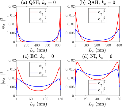
Figure 6: (Color online) Probability distributions of the edge states for the Floquet Hamiltonian of the HgTe/(Hg,Cd)Te with different sizes $L_{y}$ under $k_{x}=0$. The other parameters are the same as those in Fig. 1. Notice that the subscript $-$ denotes the edge states of $E_{\sigma-}$ with $\sigma=\uparrow,\downarrow$.

It is indicated in Fig. 6 that the probability distributions of the edge states for the $-$ bands $E_{\sigma-}$ have similar properties as those for the $+$ bands $E_{\sigma+}$ with changing system size $L_{y}$.

References

• Kane and Mele (2005a) C. L. Kane and E. J. Mele, “${Z}_{2}$ topological order and the quantum spin hall effect,” Phys. Rev. Lett. 95, 146802 (2005a).
• Kane and Mele (2005b) Charles L Kane and Eugene J Mele, “Quantum spin hall effect in graphene,” Physical review letters 95, 226801 (2005b).
• Abergel (2018) David Abergel, “Hot quantum spin hall effect,” Nature Physics 14, 108–108 (2018).
• Bernevig et al. (2006) B Andrei Bernevig, Taylor L Hughes,  and Shou-Cheng Zhang, “Quantum spin hall effect and topological phase transition in hgte quantum wells,” science 314, 1757–1761 (2006).
• Konig et al. (2007) Markus Konig, Steffen Wiedmann, Christoph Brune, Andreas Roth, Hartmut Buhmann, Laurens W Molenkamp, Xiao-Liang Qi,  and Shou-Cheng Zhang, “Quantum spin hall insulator state in hgte quantum wells,” Science 318, 766–770 (2007).
• König et al. (2008) Markus König, Hartmut Buhmann, Laurens W. Molenkamp, Taylor Hughes, Chao-Xing Liu, Xiao-Liang Qi,  and Shou-Cheng Zhang, “The quantum spin hall effect: theory and experiment,” Journal of the Physical Society of Japan 77, 031007 (2008).
• Prodan (2009) Emil Prodan, “Robustness of the spin-chern number,” Physical Review B 80, 125327 (2009).
• Qi et al. (2008) Xiao-Liang Qi, Taylor L Hughes,  and Shou-Cheng Zhang, “Topological field theory of time-reversal invariant insulators,” Physical Review B 78, 195424 (2008).
• Yu et al. (2011) Rui Yu, Xiao Liang Qi, Andrei Bernevig, Zhong Fang,  and Xi Dai, “Equivalent expression of z 2 topological invariant for band insulators using the non-abelian berry connection,” Physical Review B 84, 075119 (2011).
• Lee and Ye (2015) Ching Hua Lee and Peng Ye, “Free-fermion entanglement spectrum through wannier interpolation,” Physical Review B 91, 085119 (2015).
• Zhou et al. (2008) Bin Zhou, Hai-Zhou Lu, Rui-Lin Chu, Shun-Qing Shen,  and Qian Niu, “Finite size effects on helical edge states in a quantum spin-hall system,” Physical review letters 101, 246807 (2008).
• Liu et al. (2010) Chao-Xing Liu, HaiJun Zhang, Binghai Yan, Xiao-Liang Qi, Thomas Frauenheim, Xi Dai, Zhong Fang,  and Shou-Cheng Zhang, “Oscillatory crossover from two-dimensional to three-dimensional topological insulators,” Phys. Rev. B 81, 041307 (2010).
• Fu et al. (2014) Hua-Hua Fu, Jing-Tao Lü,  and Jin-Hua Gao, “Finite-size effects in the quantum anomalous hall system,” Physical Review B 89, 205431 (2014).
• Li et al. (2009) Jian Li, Rui-Lin Chu, Jainendra K Jain,  and Shun-Qing Shen, “Topological anderson insulator,” Physical review letters 102, 136806 (2009).
• Jiang et al. (2009) Hua Jiang, Lei Wang, Qing-feng Sun,  and XC Xie, “Numerical study of the topological anderson insulator in hgte/cdte quantum wells,” Physical Review B 80, 165316 (2009).
• Groth et al. (2009) CW Groth, M Wimmer, AR Akhmerov, J Tworzydło,  and CWJ Beenakker, “Theory of the topological anderson insulator,” Physical review letters 103, 196805 (2009).
• Xing et al. (2011) Yanxia Xing, Lei Zhang,  and Jian Wang, “Topological anderson insulator phenomena,” Physical Review B 84, 035110 (2011).
• Li et al. (2011) Wei Li, Jiadong Zang,  and Yongjin Jiang, “Size effects on transport properties in topological anderson insulators,” Physical Review B 84, 033409 (2011).
• Ning et al. (2022) Zhen Ning, Baobing Zheng, Dong-Hui Xu,  and Rui Wang, “Photoinduced quantum anomalous hall states in the topological anderson insulator,” Physical Review B 105, 035103 (2022).
• Calvo et al. (2015) Hernan Laureano Calvo, LEF Foa Torres, Pablo Matías Perez-Piskunow, Carlos Antonio Balseiro,  and Gonzalo Usaj, “Floquet interface states in illuminated three-dimensional topological insulators,” Physical Review B 91, 241404 (2015).
• Zhu et al. (2014) Hua-Xin Zhu, Tong-Tong Wang, Jin-Song Gao, Shuai Li, Ya-Jun Sun,  and Gui-Lin Liu, “Floquet topological insulator in the bhz model with the polarized optical field,” Chinese Physics Letters 31, 030503 (2014).
• Qin et al. (2022a) Fang Qin, Rui Chen,  and Hai-Zhou Lu, “Phase transitions in intrinsic magnetic topological insulator with high-frequency pumping,” Journal of Physics: Condensed Matter 34, 225001 (2022a).
• Liu et al. (2021) Xiaoyu Liu, Peizhe Tang, Hannes Hübener, Umberto De Giovannini, Wenhui Duan,  and Angel Rubio, “Floquet engineering of magnetism in topological insulator thin films,” arXiv preprint arXiv:2106.06977  (2021).
• Li et al. (2010) Huichao Li, L Sheng, DN Sheng,  and DY Xing, “Chern number of thin films of the topological insulator bi2se3,” Physical Review B 82, 165104 (2010).
• Dabiri et al. (2021) S Sajad Dabiri, Hosein Cheraghchi,  and Ali Sadeghi, “Light-induced topological phases in thin films of magnetically doped topological insulators,” Physical Review B 103, 205130 (2021).
• Dabiri and Cheraghchi (2021) S Sajad Dabiri and Hosein Cheraghchi, “Engineering of topological phases in driven thin topological insulators: Structure inversion asymmetry effect,” Physical Review B 104, 245121 (2021).
• Pervishko et al. (2018) Anastasiia A Pervishko, Dmitry Yudin,  and Ivan A Shelykh, “Impact of high-frequency pumping on anomalous finite-size effects in three-dimensional topological insulators,” Physical Review B 97, 075420 (2018).
• Zhu et al. (2022) Tongshuai Zhu, Huaiqiang Wang,  and Haijun Zhang, “Floquet engineering of magnetic topological insulator mnbi2te4 films,” arXiv preprint arXiv:2210.12457  (2022).
• Haldane (1988) F Duncan M Haldane, “Model for a quantum hall effect without landau levels: Condensed-matter realization of the" parity anomaly",” Physical review letters 61, 2015 (1988).
• Chang et al. (2013) Cui-Zu Chang, Jinsong Zhang, Xiao Feng, Jie Shen, Zuocheng Zhang, Minghua Guo, Kang Li, Yunbo Ou, Pang Wei, Li-Li Wang, et al., “Experimental observation of the quantum anomalous hall effect in a magnetic topological insulator,” Science 340, 167–170 (2013).
• Yu et al. (2010) Rui Yu, Wei Zhang, Hai-Jun Zhang, Shou-Cheng Zhang, Xi Dai,  and Zhong Fang, “Quantized anomalous hall effect in magnetic topological insulators,” science 329, 61–64 (2010).
• Linder et al. (2009) Jacob Linder, Takehito Yokoyama,  and Asle Sudbø, “Anomalous finite size effects on surface states in the topological insulator bi 2 se 3,” Physical review B 80, 205401 (2009).
• Lu et al. (2013) Hai-Zhou Lu, An Zhao,  and Shun-Qing Shen, “Quantum transport in magnetic topological insulator thin films,” Physical review letters 111, 146802 (2013).
• Lu et al. (2010) Hai-Zhou Lu, Wen-Yu Shan, Wang Yao, Qian Niu,  and Shun-Qing Shen, “Massive dirac fermions and spin physics in an ultrathin film of topological insulator,” Physical review B 81, 115407 (2010).
• Shan et al. (2010) Wen-Yu Shan, Hai-Zhou Lu,  and Shun-Qing Shen, “Effective continuous model for surface states and thin films of three-dimensional topological insulators,” New Journal of Physics 12, 043048 (2010).
• Titum et al. (2015) Paraj Titum, Netanel H Lindner, Mikael C Rechtsman,  and Gil Refael, “Disorder-induced floquet topological insulators,” Physical review letters 114, 056801 (2015).
• Lee and Song (2021) Ching Hua Lee and Justin CW Song, “Quenched topological boundary modes can persist in a trivial system,” Communications Physics 4, 1–8 (2021).
• Li et al. (2018) Linhu Li, Ching Hua Lee,  and Jiangbin Gong, “Realistic floquet semimetal with exotic topological linkages between arbitrarily many nodal loops,” Physical review letters 121, 036401 (2018).
• Lee et al. (2018) Ching Hua Lee, Wen Wei Ho, Bo Yang, Jiangbin Gong,  and Zlatko Papić, “Floquet mechanism for non-abelian fractional quantum hall states,” Physical review letters 121, 237401 (2018).
• Yap et al. (2018) Han Hoe Yap, Longwen Zhou, Ching Hua Lee,  and Jiangbin Gong, “Photoinduced half-integer quantized conductance plateaus in topological-insulator/superconductor heterostructures,” Physical Review B 97, 165142 (2018).
• Chan et al. (2016) Ching-Kit Chan, Yun-Tak Oh, Jung Hoon Han,  and Patrick A Lee, “Type-ii weyl cone transitions in driven semimetals,” Physical Review B 94, 121106 (2016).
• Bonasera et al. (2022) F. Bonasera, S.-B. Zhang, L. Privitera,  and F. M. D. Pellegrino, “Tunable interface states between floquet-weyl semimetals,” Phys. Rev. B 106, 195115 (2022).
• Oka and Aoki (2009) Takashi Oka and Hideo Aoki, “Photovoltaic hall effect in graphene,” Physical Review B 79, 081406 (2009).
• Sato et al. (2019) SA Sato, JW McIver, M Nuske, P Tang, G Jotzu, B Schulte, H Hübener, U De Giovannini, L Mathey, MA Sentef, et al., “Microscopic theory for the light-induced anomalous hall effect in graphene,” Physical Review B 99, 214302 (2019).
• McIver et al. (2020) James W McIver, Benedikt Schulte, F-U Stein, Toru Matsuyama, Gregor Jotzu, Guido Meier,  and Andrea Cavalleri, “Light-induced anomalous hall effect in graphene,” Nature physics 16, 38–41 (2020).
• Sentef et al. (2015) MA Sentef, M Claassen, AF Kemper, B Moritz, T Oka, JK Freericks,  and TP Devereaux, “Theory of floquet band formation and local pseudospin textures in pump-probe photoemission of graphene,” Nature communications 6, 7047 (2015).
• Broers and Mathey (2022) Lukas Broers and Ludwig Mathey, “Detecting light-induced floquet band gaps of graphene via trarpes,” Physical Review Research 4, 013057 (2022).
• Candussio et al. (2022) S Candussio, S Bernreuter, T Rockinger, K Watanabe, T Taniguchi, J Eroms, IA Dmitriev, D Weiss,  and SD Ganichev, “Terahertz radiation induced circular hall effect in graphene,” Physical Review B 105, 155416 (2022).
• Qin et al. (2022b) Tao Qin, Pengfei Zhang,  and Guoao Yang, “Nondiagonal disorder enhanced topological properties of graphene with laser irradiation,” Physical Review B 105, 184203 (2022b).
• Cupo et al. (2021) Andrew Cupo, Emilio Cobanera, James D Whitfield, Chandrasekhar Ramanathan,  and Lorenza Viola, “Floquet graphene antidot lattices,” Physical Review B 104, 174304 (2021).
• Assi et al. (2021) IA Assi, JPF LeBlanc, Martin Rodriguez-Vega, Hocine Bahlouli,  and Michael Vogl, “Floquet engineering and nonequilibrium topological maps in twisted trilayer graphene,” Physical Review B 104, 195429 (2021).
• Luo (2021) Ma Luo, “Tuning of a bilayer graphene heterostructure by horizontally incident circular polarized light,” Physical Review B 103, 195422 (2021).
• Schüler et al. (2020) Michael Schüler, Umberto De Giovannini, Hannes Hübener, Angel Rubio, Michael A Sentef, Thomas P Devereaux,  and Philipp Werner, “How circular dichroism in time-and angle-resolved photoemission can be used to spectroscopically detect transient topological states in graphene,” Physical Review X 10, 041013 (2020).
• Topp et al. (2019) Gabriel E. Topp, Gregor Jotzu, James W. McIver, Lede Xian, Angel Rubio,  and Michael A. Sentef, “Topological floquet engineering of twisted bilayer graphene,” Phys. Rev. Research 1, 023031 (2019).
• Rodriguez-Vega et al. (2020) Martin Rodriguez-Vega, Michael Vogl,  and Gregory A Fiete, “Floquet engineering of twisted double bilayer graphene,” Physical Review Research 2, 033494 (2020).
• Li et al. (2020) Yantao Li, HA Fertig,  and Babak Seradjeh, “Floquet-engineered topological flat bands in irradiated twisted bilayer graphene,” Physical Review Research 2, 043275 (2020).
• Berdakin et al. (2021) Matías Berdakin, Esteban A Rodríguez-Mena,  and Luis EF Foa Torres, “Spin-polarized tunable photocurrents,” Nano Letters 21, 3177–3183 (2021).
• Dal Lago et al. (2017) Virginia Dal Lago, E Suárez Morell,  and LEF Foa Torres, “One-way transport in laser-illuminated bilayer graphene: A floquet isolator,” Physical Review B 96, 235409 (2017).
• Huamán et al. (2021) A Huamán, LEF Foa Torres, CA Balseiro,  and Gonzalo Usaj, “Quantum hall edge states under periodic driving: A floquet induced chirality switch,” Physical Review Research 3, 013201 (2021).
• Rothe et al. (2010) DG Rothe, RW Reinthaler, CX Liu, LW Molenkamp, SC Zhang,  and EM Hankiewicz, “Fingerprint of different spin-orbit terms for spin transport in hgte quantum wells,” New Journal of Physics 12, 065012 (2010).
• Qi et al. (2006) Xiao-Liang Qi, Yong-Shi Wu,  and Shou-Cheng Zhang, “Topological quantization of the spin hall effect in two-dimensional paramagnetic semiconductors,” Physical Review B 74, 085308 (2006).
• Qi and Zhang (2011) Xiao-Liang Qi and Shou-Cheng Zhang, “Topological insulators and superconductors,” Reviews of Modern Physics 83, 1057–1110 (2011).
• Chen et al. (2019) Rui Chen, Chui-Zhen Chen, Bin Zhou,  and Dong-Hui Xu, “Finite-size effects in non-hermitian topological systems,” Physical Review B 99, 155431 (2019).
• Trevisan et al. (2022) Thaís V. Trevisan, Pablo Villar Arribi, Olle Heinonen, Robert-Jan Slager,  and Peter P. Orth, “Bicircular light floquet engineering of magnetic symmetry and topology and its application to the dirac semimetal ${\mathrm{cd}}_{3}{\mathrm{as}}_{2}$,” Physical review letters 128, 066602 (2022).
• Chen et al. (2018a) Rui Chen, Bin Zhou,  and Dong-Hui Xu, “Floquet weyl semimetals in light-irradiated type-ii and hybrid line-node semimetals,” Physical Review B 97, 155152 (2018a).
• Chen et al. (2018b) Rui Chen, Dong-Hui Xu,  and Bin Zhou, “Floquet topological insulator phase in a weyl semimetal thin film with disorder,” Physical Review B 98, 235159 (2018b).
• Du et al. (2022) Xiu-Li Du, Rui Chen, Rui Wang,  and Dong-Hui Xu, “Weyl nodes with higher-order topology in an optically driven nodal-line semimetal,” Physical Review B 105, L081102 (2022).
• Wang et al. (2022) Zi-Ming Wang, Rui Wang, Jin-Hua Sun, Ting-Yong Chen,  and Dong-Hui Xu, “Floquet weyl semimetal phases in light-irradiated higher-order topological dirac semimetals,” arXiv preprint arXiv:2210.01012  (2022).
• Jangjan and Hosseini (2020) Milad Jangjan and Mir Vahid Hosseini, “Floquet engineering of topological metal states and hybridization of edge states with bulk states in dimerized two-leg ladders,” Scientific Reports 10, 14256 (2020).
• Jangjan and Hosseini (2021) Milad Jangjan and Mir Vahid Hosseini, “Topological phase transition between a normal insulator and a topological metal state in a quasi-one-dimensional system,” Scientific reports 11, 12966 (2021).
• Michetti et al. (2012) P Michetti, PH Penteado, JC Egues,  and P Recher, “Helical edge states in multiple topological mass domains,” Semiconductor Science and Technology 27, 124007 (2012).
• Yang et al. (2011) Yunyou Yang, Zhong Xu, L Sheng, Baigeng Wang, DY Xing,  and DN Sheng, “Time-reversal-symmetry-broken quantum spin hall effect,” Physical review letters 107, 066602 (2011).
• Chen et al. (2017) Rui Chen, Dong-Hui Xu,  and Bin Zhou, “Disorder-induced topological phase transitions on lieb lattices,” Physical Review B 96, 205304 (2017).
• Landauer (1970) Rolf Landauer, “Electrical resistance of disordered one-dimensional lattices,” Philosophical magazine 21, 863–867 (1970).
• Büttiker (1988) Markus Büttiker, “Absence of backscattering in the quantum hall effect in multiprobe conductors,” Physical Review B 38, 9375 (1988).
• Qiu et al. (2022) Gang Qiu, Peng Zhang, Peng Deng, Su Kong Chong, Lixuan Tai, Christopher Eckberg,  and Kang L Wang, “Mesoscopic transport of quantum anomalous hall effect in the submicron size regime,” Physical Review Letters 128, 217704 (2022).
• Zhou et al. (2022) Ling-Jie Zhou, Ruobing Mei, Yi-Fan Zhao, Ruoxi Zhang, Deyi Zhuo, Zi-Jie Yan, Wei Yuan, Morteza Kayyalha, Moses HW Chan, Chao-Xing Liu, et al., “Confinement-induced chiral edge channel interaction in quantum anomalous hall insulators,” arXiv preprint arXiv:2207.08371  (2022).
• Zhao et al. (2020) Yi-Fan Zhao, Ruoxi Zhang, Ruobing Mei, Ling-Jie Zhou, Hemian Yi, Ya-Qi Zhang, Jiabin Yu, Run Xiao, Ke Wang, Nitin Samarth, et al., “Tuning the chern number in quantum anomalous hall insulators,” Nature 588, 419–423 (2020).
• Zhao et al. (2022) Yi-Fan Zhao, Ruoxi Zhang, Ling-Jie Zhou, Ruobing Mei, Zi-Jie Yan, Moses HW Chan, Chao-Xing Liu,  and Cui-Zu Chang, “Zero magnetic field plateau phase transition in higher chern number quantum anomalous hall insulators,” Physical Review Letters 128, 216801 (2022).
• Shen (2012) Shun-Qing Shen, Topological insulators, Vol. 174 (Springer-Verlag Berlin Heidelberg, 2012).