Global impact of emerging internetwork fields on the low solar atmosphere

Abstract

Small-scale, newly emerging internetwork (IN) magnetic fields are considered a viable source of energy and mass for the solar chromosphere and possibly the corona. Multiple studies show that single events of flux emergence can indeed locally heat the low solar atmosphere through interactions of the upward propagating magnetic loops and the preexisting ambient field lines. However, the global impact of the newly emerging IN fields on the solar atmosphere is still unknown. In this letter we study the spatio-temporal evolution of IN bipolar flux features and analyze their impact on the energetics and dynamics of the quiet Sun (QS) atmosphere. We use high resolution, multi-wavelength, coordinated observations obtained with the Interface Region Imaging Spectrograph (IRIS), Hinode and the Atmospheric Imaging Assembly (AIA) to identify emerging IN magnetic fields and follow their evolution. Our observational results suggest that only the largest IN bipoles are capable of heating locally the low solar atmosphere, while the global contribution of these bipoles appears to be marginal. However, the total number of bipoles detected and their impact estimated in this work is limited by the sensitivity level, spatial resolution, and duration of our observations. To detect smaller and weaker IN fields that would maintain the basal flux, and examine their contribution to the chromospheric heating, we will need higher resolution, higher sensitivity and longer time series obtained with current and next-generation ground- and space-based telescopes.

1 Introduction

Internetwork (IN) magnetic fields are dynamic magnetic structures that populate the interior of supergranular cells (Livingston & Harvey, 1975; Smithson, 1975). They are spread all over the Sun (Wang et al., 1995), maintain the photospheric network (Gošić et al., 2014), and may hold a significant fraction of the total magnetic energy stored at the solar surface (Trujillo Bueno et al., 2004). For these reasons IN fields are considered to be the main building blocks of the quiet Sun (QS) magnetism (see Bellot Rubio & Orozco Suárez 2019 for a review).

Recent Hinode observations showed that IN fields mainly appear in the form of magnetic bipoles in the photosphere (Gošić et al., 2022), likely generated by small-scale surface dynamo (Rempel, 2014). According to some numerical models (Isobe et al., 2008; Amari et al., 2015; Moreno-Insertis et al., 2018), and observations (e.g., Martínez González & Bellot Rubio, 2009; Martínez González et al, 2010; Gošić et al., 2021), these fields may upon appearance in the photosphere rise through the lower atmospheric layers, and locally heat the chromosphere and transition region.

Considering the magnetic and energy budget of IN fields, it is therefore important to determine the global contribution of the emerging IN fields to the dynamics and energetics of the chromosphere and the atmospheric layers above. This open question has not yet been addressed in detail, using high resolution observations that simultaneously cover the solar atmosphere from the photospheric to coronal heights. The main reason for this was the lack of suitable observations and the need for sophisticated analysis that allows to identify footpoints of magnetic loops, and determine their history in a reliable way. Such observations at the photospheric level are provided by the Narrowband Filter Imager (NFI; Tsuneta et al., 2008) aboard the Hinode satellite (Kosugi et al., 2007), and at the chromospheric/transition region and coronal levels by the Interface Region Imaging Spectrograph (IRIS; De Pontieu et al., 2014) and the Atmospheric Imaging Assembly (AIA; Lemen et al., 2012) onboard the Solar Dynamics Observatory (SDO; Pesnell et al., 2012). Furthermore, to understand the impact of newly emerging IN fields on the chromospheric energy balance, one would need to determine the thermodynamic properties from chromospheric lines, considering the non-local thermodynamic equilibrium (non-LTE) radiative transfer. Diagnosing chromospheric conditions requires inversion codes that are typically slow and difficult to use. In this work we will take advantage of a new approach that solves these issues through a combination of machine learning and classical inversion techniques to speed up and facilitate the recovery of thermodynamical information from the solar spectra (e.g., Sainz Dalda et al., 2019).

The main goal in this letter is to establish the global impact of the newly emerging IN fields on the lower solar atmosphere. We address this open question by employing coordinated, multi-wavelength IRIS, Hinode and SDO observations. These instruments allow us to study the spatio-temporal evolution of the QS fields at high spatial, spectral, and temporal resolution, while observing the solar atmosphere from the photosphere up to the transition region and corona.

The observations used in this paper are described in Section 2. The identification, classification and tracking of IN bipolar flux features is explained in Section 3. Section 4 provides the results, while conclusions are given in Section 5.

2 Observations and data processing

The observations used in this work were obtained on 2013 March 23. IRIS measurements start at 07:09:49 UT and end at 12:05:37 UT. Hinode data set covers this interval from 08:04:38 UT to 10:59:36 UT. The observations show the spatial and temporal evolution of a QS region at the disk center.

IRIS data set is a medium-sit-and-stare raster, taking spectra in the near ultraviolet (NUV) band in the wavelength range from 2790 Å to 2835 Å. The NUV spectroscopic measurements sample the solar atmosphere from the photosphere to the upper chromosphere. The spectra are recorded every 5 seconds along a slit length of $60$″. Slit-jaw images (pixel size is $0\farcs 16$) were taken using the C II 1330 Å (SJI 1330), Si IV 1400 Å (SJI 1400), Mg II k 2796 Å (SJI 2796), and Mg II h wing at 2832 Å (SJI 2832) filters, compensating for the solar rotation. The cadence of the slit-jaw images are 18 s, 15 s, 15 s, and 89 s, respectively. The IRIS data were corrected for dark current, flat-field, geometric distortion, and scattered light (Wülser et al., 2018).

Using the IRIS² inversion code (Sainz Dalda et al., 2019) we derived the thermodynamical properties of the observed QS atmosphere as a function of the optical depth. The code employs the k-means clustering method to build a database of the representative IRIS Mg II h and k spectral profiles (RP) and the corresponding atmospheric models. These RPs were inverted with the STiC code (de la Cruz Rodríguez et al., 2016, 2019). For each observed Mg II h and k pair, IRIS² assigns the model atmosphere resulting from the inversion of the closest RP to the observed profiles.

The NFI was employed in shutterless mode to obtain the full Stokes vector in the photospheric Fe I 5250 Å line at 2 wavelength positions from the line center. These observations provide circular and linear polarization maps, showing photospheric activity of the vertical (loop footpoints) and horizontal (loop tops) components of magnetic fields, respectively. After the data reduction process and co-alignment of Hinode and IRIS observations, the effective field of view (FOV) was reduced to $35\arcsec\times 60\arcsec$ (the pixel size is $0\farcs 16$), which is sufficient to capture the evolution of at least two supergranular cells for two hours and 40 minutes at a cadence of $\sim 60$ s. This allows us to track the temporal evolution of IN fields in a magnetogram sequence that considerably exceeds the mean lifetime of IN magnetic structures on granular scales. Magnetograms $M$ were calculated in the standard way using the Stokes $I$ and $V$ filtergrams:

$$M=\frac{1}{2}\left(\frac{V_{\text{blue}}}{I_{\text{blue}}}-\frac{V_{\text{red}}}{I_{\text{red}}}\right),$$ (1)

where “blue” indicates the measurements in the blue wing of the line and “red” in the red wing. The linear polarization maps $\rm LP$ are computed as ${\rm LP}=\sum_{i=1}^{2}\sqrt{Q(\lambda_{i})^{2}+U(\lambda_{i})^{2}}/I(\lambda_{i})/2$. All magnetogram and LP maps were smoothed using a $3\times 3$ Gaussian-type spatial kernel to reduce the noise, and the five-minute oscillations were removed from the maps by applying a subsonic filter (Title et al., 1989; Straus et al., 1992).

Figure 1: From left to right: Hinode/NFI magnetograms and linear polarization maps, IRIS SJI 1400 and IRIS SJI 2796 slit-jaw images. The detected bipoles are enclosed with contours of different colors. Regions 1, 2, and 3 (red ellipses) show the largest emerging cluster of magnetic elements, one small-scale IN loop, and a NW patch that originate from a previously emerged IN bipolar system. The animation of this figure runs from $\Delta t$=0:00:00 to $\Delta t$=2:36:45.
(An animation of this figure is available.)

We also make use of the Helioseismic and Magnetic Imager (HMI; Scherrer et al., 2012) and AIA observations. This allows us to determine the evolution of the observed QS region before the IRIS and Hinode observations started and to examine emission at coronal heights.

The alignment of the datasets was carried out by compensating for solar rotation and scaling all images to match the IRIS pixel size. All IRIS, Hinode and SDO sequences were interpolated in time applying the nearest neighbor method of interpolation to match the cadence of the SJI 2796 images (15 s). Images are then aligned comparing prominent network (NW) features and bright points in IRIS SJI 2832 images with the Hinode intensity filtergrams and AIA 1600 Å channel.

3 Identification and tracking of internetwork bipoles

To detect IN magnetic bipoles (loops and clusters) and separate them from the unipolar fields (isolated flux concentrations), we first identified all individual magnetic features in the magnetograms and LP maps. We consider loops to represent two circular polarization patches (positive and negative polarity footpoints) moving away from each other, while flux clusters consist of two or more patches that emerge within a short time interval in a relatively small area.

Using the YAFTA code and the downhill identification method (Welsch & Longcope, 2003), we automatically tracked all the detected flux patches to determine their spatio-temporal evolution. This process includes identifications of all merging, fragmentation and cancellation events that magnetic patches may undergo during their lifetimes. In this way, we can determine the history of every detected magnetic feature. Real features in the magnetograms are separated from the background signal by setting a flux density threshold to $2\sigma$ (10 Mx cm^-2). This allows as to detect more faint magnetic elements, considering all of them to be real if their minimum size is at least 4 pixels and they live two frames or more. Magnetic features that appear and disappear in situ and are visible in only one frame are discarded. The reason is that those flux patches may just represent intrinsic flux fluctuations around the threshold level.

The appearance of loop footpoints and clusters in the photosphere is preceded by LP signal between footpoints that move away from each other. Therefore, magnetic bipoles are identified by searching for all LP signals (loop tops) that are followed by pairs of opposite-polarity flux features that appear in situ (loop footpoints). To be selected, these footpoints have to appear within 6 minutes after the first one becomes visible in a magnetogram, and they have to move away from each other. Although clusters bring numerous magnetic patches to the solar surface, they follow the same pattern of the spatio-temporal evolution as loops, i.e., flux features move away from each other with respect to their common center of appearance. Usually, there are multiple LP patches within clusters. The tracking and identification of IN bipoles in this work is similar to the method described in Gošić et al. (2022), the main difference being that here we use the NFI LP maps instead of extrapolations of the magnetic field lines to identify the loop tops.

For the strongest flux patches visible in the first frame, we cannot determine their history from the NFI magnetograms. Thus, we used HMI data to determine if they appear as unipolar or bipolar structures. This is important because the strongest magnetic elements may have a considerable impact on the lower solar atmosphere. Since HMI is not sensitive to the weakest IN patches, we classified as bipoles only those flux patches that are clearly resolved and appear in situ, following the expected pattern of flux emergence.

Figure 2: Temperature spatio-temporal map from the IRIS² inversions at $\log_{10}\tau_{500}=-5.8$. The white boxes indicate locations and times when the emerging IN bipoles were under the IRIS slit.

Figure 3: From left to right: Hinode/NFI magnetogram, AIA 304 Å, AIA 171 Å, and AIA 193 Å images. The detected IN bipoles are enclosed with contours having different colors. Regions 1, 2, and 3 marked with the red ellipses show the same as in Figure 1. The animation of this figure runs from $\Delta t$=0:00:00 to $\Delta t$=2:36:45.
(An animation of this figure is available.)

4 Results

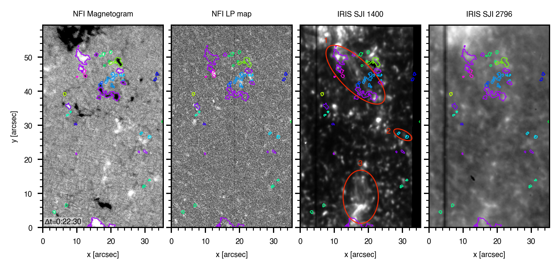
Using HMI and Hinode/NFI magnetograms we identified and tracked the spatio-temporal evolution of individual magnetic elements representing footpoints of $161$ bipolar structures (IN loops and clusters of magnetic elements). This translates into an emergence rate of $\sim 0.038$ bipoles per hour and arcsec², which is in agreement with the results reported by Gošić et al. (2022). If we take into account the total area occupied by the footpoints, only $2\%$ of the available FOV at any given time is covered by bipolar IN fields. Note that this ratio depends on spatial resolution, magnetic sensitivity, and intrinsic fluctuations of the total instantaneous unsigned IN flux (e.g., Gošić et al., 2022). The two largest bipoles whose footpoints are visible in the first NFI magnetogram are identified employing HMI data. They are marked in Figure 1 with violet contours inside the encircled region 1 (red ellipse) and at the bottom of the FOV at $(x,y)=(16\arcsec,0\arcsec)$. By the time Hinode/NFI started to observe, most of the footpoints of the two clusters either transformed into NW features or canceled with the opposite polarity NW elements. The tracking results can be evaluated with the animation accompanying Figure 1, which shows all the magnetic bipoles (left panel) detected in our Hinode/NFI magnetograms. Flux patches belonging to the same bipole have the same colors. The corresponding contours are overplotted on the LP maps, SJI 1400 and SJI 2796 images, from left to right, respectively.

To detect chromospheric activity related to the newly emerging IN fields, we used SJI 1400 and 2796 images. As can be seen from Figure 1 and the accompanying movie, the strongest emission in both filtergram sequences is co-spatial with strong magnetic elements, i.e., large clusters and the positive- and negative- polarity NW elements centered at $(x,y)=(16\arcsec,0\arcsec)$ and $(x,y)=(10\arcsec,56\arcsec)$, respectively. The rest of the FOV is overwhelmed by bright features. We determined that $\sim 90\%$ of the detected bipoles overlap with IRIS brightenings in SJI 1400 that are identified considering all the pixels with the signal above a threshold level of 60 counts per pixel, as in Gošić et al. (2018). We remind the reader that the SJI 1400 filter is sensitive to emission from the transition region Si IV 1394/1403 Å lines and continuum formed in the upper photosphere/lower chromosphere. Therefore, most of the SJI 1400 bright patches in the QS regions are formed in the chromosphere due to upward propagating acoustic waves in non-magnetic environment (Martínez-Sykora et al., 2015). When we apply a subsonic filter to remove those short-lived (two minutes) bright grains, the overlap between the IN bipoles and IRIS SJI 1400 brightenings drops to $\sim 60\%$, suggesting that many small-scale IN loops and clusters do not perturb the chromospheric layers.

By visual inspection of IRIS SJI features above the detected bipoles, we determined that the bipoles are either embedded in regions with already ongoing activities in the chromosphere or the overlapping IRIS SJI 1400 brightenings ($\sim 60\%$) above them do not seem to be different from the background activity (for example the loop inside region 2 in the SJI 1400 panel in Figures 1 and 3). This scenario applies to all other clusters, except for the strongest clusters (regions 1 and 3). The southern positive polarity magnetic element ($(x,y)=(16\arcsec,0\arcsec)$) locally impacts the chromosphere through interactions with the surrounding opposite-polarity flux features. Numerous dynamic and episodic bright loops and grains can be seen around this footpoint, probably energized by reconnection of the magnetic field lines of the footpoint and the surrounding flux patches.

The cluster within region 1 exhibits the temporal and spatial evolution similar to the cluster described in Gošić et al. (2021). The footpoints expanded with time and started interacting with the negative polarity NW patches in the north. Eventually the region produced a surge-like event around $\Delta t$=00:25:30, (onset at $\Delta t$=00:22:30), which is expected to be observed when new and preexisting fields reconnect (Guglielmino et al., 2018; Nóbrega-Siverio et al., 2017).

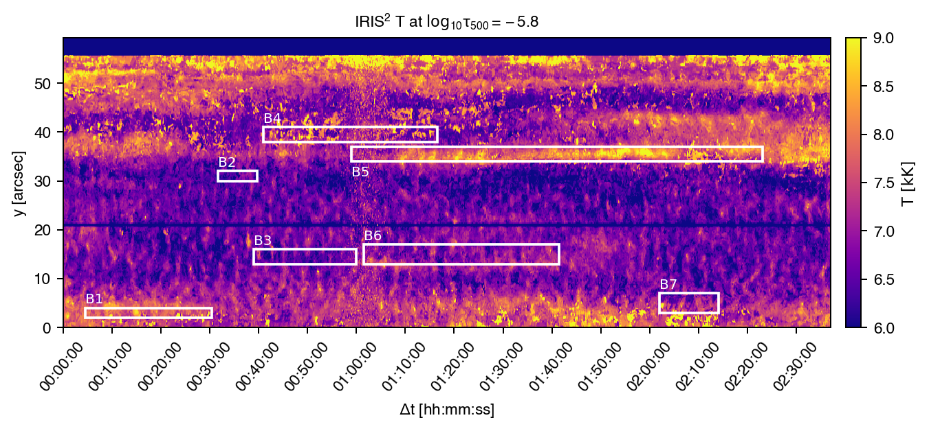
Figure 2 shows the temperature map derived from IRIS² inversions. The IRIS slit covered seven emerging bipoles. Five of them are embedded in the background activity and do not perturb the chromosphere. They do not produce any excess emission neither in the IRIS NUV nor FUV spectral lines. The bipole labeled as B4, is co-spatial with increased temperature, but this is likely due to cancellation with the opposite polarity magnetic features in its vicinity (Gošić et al., 2018). Only a few bipoles can be associated with the chromospheric activity. For example, the negative polarity footpoint (B5), clearly shows an increase of the chromospheric temperature. This magnetic element eventually becomes an NW element. Bipole B1 emerges next to an ongoing cancellation event (hence a higher temperature before the bipole emerged), with which the positive footpoint starts interacting and eventually completely disappears. This cancellation maintained an increased temperature in that region for the next 26 minutes. Another intriguing event is B2 loop that shows a slight temperature increase towards the end of the white box. This is probably the result of an upward propagating wave because we do not see any activity above the footpoints in the filtered IRIS slit-jaw images. In addition, this is a small, short-lived loop (8 minutes), so it is unlikely that in such a short time this loop can reach the chromosphere.

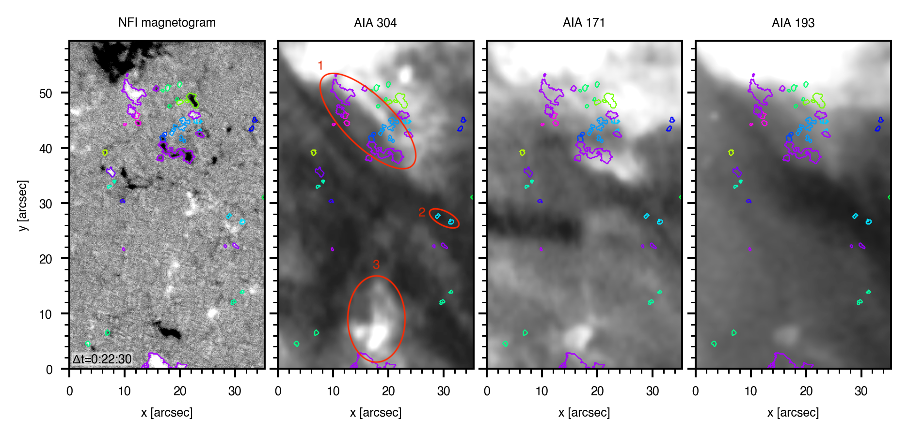
Very limited activity in the lower solar atmosphere within the observed QS region is also apparent in the AIA filtergrams displayed in Fig 3. The AIA 304 Å, 171 Å and 193 Å channels show the chromospheric (304 Å) and coronal (171 Å and 193 Å) activity inside regions 1 and 3. The rest of the FOV looks very quiet with some long loops extended across the FOV that originate in an active region in the north (not visible in the Hinode and IRIS observations).

5 Conclusions

In this work we used Hinode/NFI, IRIS and SDO/AIA observations to detect newly emerging IN bipoles in the solar photosphere and estimate the global and direct contribution of emerging fields on the chromospheric dynamics and energetics. Our results suggest that the majority ($\sim 98\%$ based on the SJI 1400 activity) of bipolar IN structures do not have enough magnetic buoyancy nor live long enough to rise through the solar atmosphere and directly affect the solar chromosphere and beyond. This result should be understood as a minimum. More active QS regions may generate stronger emerging fields capable of rising through the solar atmosphere. Also, our statistics could have been different had we identified more bipoles under the slit, which will be possible in future with multislit instrument such as MUSE (De Pontieu et al., 2020). In the meantime, if we consider only the bipoles under the slit, despite of the small sample, then $40\%$ of the loops may heat the chromosphere either through reconnection with the overlying magnetic fields or through cancellation with the surrounding flux patches.

Based on our observations, only the strongest three detected bipoles produced local temperature increase in the chromosphere. They are also capable of generating surge-like phenomena through reconnection of their magnetic field lines with the preexisting fields. We conclude that newly emerging IN bipoles, at the sensitivity levels and spatial resolution of Hinode/NFI magnetograms, cannot globally maintain the chromospheric heating in a direct way through interaction with the ambient overlying magnetic fields. We either do not see a lot of evidence of heating, except for larger events, or the large events are too sporadic in space and time to considerably support the chromospheric heating. It would be interesting to study longer-duration events to increase the statistical sample that can be studied under the slit. We also note that our analysis has been focused on detecting changes in emission or chromospheric temperature as a result of the detected emergence of IN magnetic elements. We did not investigate a scenario in which the continual emergence of undetected or undetectable IN elements leads to a steady heating of the atmosphere or continuous background emission. The results presented in this letter also do not exclude a possibility that the footpoints of IN bipoles may possibly contribute to the chromospheric heating indirectly through other mechanisms such as magneto-acoustic waves and shocks, braiding of the magnetic field lines, swirls or cancellations with the opposite polarity fields in the intergranular lanes.

To better understand the smallest and weakest QS fields, we will need long duration observations with higher spatial resolution and sensitivity. Such observations are, for example, achievable with the Daniel K. Inouye Solar Telescope (DKIST; Elmore et al., 2014), and from space with the Solar Orbiter’s Polarimetric and Helioseismic Imager (Solanki et al., 2020). These instruments may detect and resolve fields that are not accessible to the currently available telescopes, but they may be continuously emerging and contributing directly to heating through interaction with preexisting fields.

A key aspect of this issue is also to study which processes determine whether emerging IN fields rise through the solar atmosphere and transfer mass and energy. This will be investigated in detail in our future work using radiative MHD Bifrost simulations (Gudiksen et al. 2011; see also Hansteen et al. 2022, in prep.).

References

- Amari et al. (2015) Amari T., Luciani J.-F., Aly J.-J. 2015, Nature, 522, 188
- Bellot Rubio & Orozco Suárez (2019) Bellot Rubio, L. R., & Orozco Suárez, D. 2019, Living Rev. Sol. Phys.,16, 1
- de la Cruz Rodríguez et al. (2016) de la Cruz Rodríguez, J., Leenaarts, J. & Asensio Ramos, A. 2016, ApJ, 830, L30
- de la Cruz Rodríguez et al. (2019) de la Cruz Rodríguez, J., Leenaarts, J., Danilović, S., & Uitenbroek, H. 2019, , 623, A74, 2019, A&A, 623, A74
- De Pontieu et al. (2014) De Pontieu B., Title A. M., Lemen J. R., et al. 2014, Sol. Phys., The Interface Region Imaging Spectrograph (IRIS)
- De Pontieu et al. (2020) De Pontieu, B., Martínez-Sykora, J., Testa, P., et al. 2020, ApJ, 888, 3. doi:10.3847/1538-4357/ab5b03
- Elmore et al. (2014) Elmore D. F., Rimmele T., Casini R., et al. 2014, in Ground- based and Airborne Instrumentation for Astronomy V, vol. 9147 of Proc. SPIE, 914707
- Gošić et al. (2014) Gošić, M., Bellot Rubio, L.R., Orozco Suárez, D., Katsukawa, Y., and del Toro Iniesta, J.C. 2014, ApJ, 797, 49
- Gošić et al. (2018) Gošić, M., de la Cruz Rodríguez, J., De Pontieu, B., Bellot Rubio, L. R., et al. 2018, ApJ, 857, 48
- Gošić et al. (2021) Gošić, M., De Pontieu, B., Bellot Rubio, L. R., et al. 2021, ApJ, 911, 41
- Gošić et al. (2022) Gošić, M., Bellot Rubio, L. R., Cheung, M. C. M., et al. 2022, ApJ, 925, 188
- Gudiksen et al. (2011) Gudiksen, B. V., Carlsson, M., Hansteen, V. H., et al. 2011, A&A, 531, A154
- Guglielmino et al. (2018) Guglielmino, S. L., Zuccarello, F., Young, P. R., Murabito, M., & Romano, P. 2018, ApJ, 856, 127
- Isobe et al. (2008) Isobe, H., Proctor, M. R. E., & Weiss, N. O. 2008, ApJ, 679, L57
- Kosugi et al. (2007) Kosugi, T., Matsuzaki, K., Sakao, T., et al. 2007, Sol. Phys., 243, 3
- Lemen et al. (2012) Lemen, J. R., Title, A.M., David J.A., et al. 2012, Sol. Phys., 275, 17
- Livingston & Harvey (1975) Livingston, W. C., & Harvey, J. 1975, BAAS, 7, 346
- Martínez González et al (2010) Martínez González, M. J., Manso Sainz, R., Asensio Ramos, A., Bellot Rubio, L.R. 2010, ApJ, 714, L94
- Martínez González & Bellot Rubio (2009) Martínez González, M. J., & Bellot Rubio, L. R. 2009, ApJ, 700, 1391
- Martínez-Sykora et al. (2015) Martínez-Sykora, J., Rouppe van der Voort, L., Carlsson, M., et al. 2015, ApJ, 803, 44
- Moreno-Insertis et al. (2018) Moreno-Insertis, F., Martínez-Sykora, J., Hansteen, V. H., & Muñoz, D. 2018, ApJ, 859, L26
- Nóbrega-Siverio et al. (2017) Nóbrega-Siverio, D., Martínez-Sykora, J., Moreno-Insertis, F., & Rouppe van der Voort, L. 2017, ApJ, 850, 153
- Pesnell et al. (2012) Pesnell, W.D.,Thompson, B.J., & Chamberlin, P.C. 2012, Sol. Phys., 275, 3
- Rempel (2014) Rempel, M. 2014, ApJ, 789, 132
- Sainz Dalda et al. (2019) Sainz Dalda, A., de la Cruz Rodríguez, J., De Pontieu B., & Gošić, M. 2019, ApJ, 875, L18
- Scherrer et al. (2012) Scherrer, P. H., Schou, J., Bush, R. I. et al. 2012, Sol. Phys., 275, 207
- Smithson (1975) Smithson, R. C. 1975, BAAS, 7, 346
- Solanki et al. (2020) Solanki, S. K., del Toro Iniesta, J. C., Woch, J., et al. 2020, A&A, 642, A11
- Straus et al. (1992) Straus, T., Deubner, F.-L., & Fleck, B. 1992, A&A, 256, 652
- Title et al. (1989) Title, A. M., Tarbell, T. D., Topka, K. P., et al. 1989, ApJ, 336, 475
- Trujillo Bueno et al. (2004) Trujillo Bueno, J., Shchukina, N., & Asensio Ramos, A. 2004, Nature, 430, 326
- Tsuneta et al. (2008) Tsuneta, S., Ichimoto, K., & Katsukawa, Y. 2008, Sol. Phys., 249, 167
- Wang et al. (1995) Wang, J., Wang, H., & Tang, F. et al. 1995, Sol. Phys., 160, 277
- Welsch & Longcope (2003) Welsch, B. T., & Longcope, D. W. 2003, ApJ, 588, 620
- Wülser et al. (2018) Wülser, J.-P., Jaeggli, S., De Pontieu, B., et al. 2018, Sol. Phys., 293, 149