Interpretable Few-shot Learning with Online Attribute Selection

Abstract

Few-shot learning (FSL) is a challenging learning problem in which only a few samples are available for each class. Decision interpretation is more important in few-shot classification since there is a greater chance of error than in traditional classification. However, most of the previous FSL methods are black-box models. In this paper, we propose an inherently interpretable model for FSL based on human-friendly attributes. Moreover, we propose an online attribute selection mechanism that can effectively filter out irrelevant attributes in each episode. The attribute selection mechanism improves the accuracy and helps with interpretability by reducing the number of participated attributes in each episode. We propose a mechanism that automatically detects the episodes where the pool of human-friendly attributes are not adequate, and compensates by engaging learned unknown attributes. We demonstrate that the proposed method achieves results on par with black-box few-shot-learning models on four widely used datasets.

1 Introduction

In recent years, deep learning has been able to achieve impressive success in computer vision tasks including object recognition. This success heavily relies on the availability of abundant labeled examples. However, accessing sufficient data is not always possible due to the limitation and challenges in data collection and annotation. Therefore, a new learning paradigm known as few-shot learning (FSL) has been considered in which the model has to generalize to novel classes with just a few training instances [31].

FSL models are first trained on a set of base classes with abundant samples, preparing to classify novel classes with just a few examples where the base and novel classes are completely disjoint. This models human generalization ability that can effectively transfer the insight obtained from prior knowledge to future tasks with limited amount of supervision [18]. Each standard few-shot classification task is called an episode. In each episode, N distinct classes are sampled from novel classes. For each of them, K instances are sampled to form a labeled training set known as support set and an unlabeled query set which the model has to classify correctly [25]. This setting is known as N-way K-shot.

Recently, few-shot learning models have been able to achieve remarkable performance. However, they usually neglect decision interpretability. As their decision can not be interpreted by human, they are considered to be black-box models. In recent years, using black-box models in real world has drawn growing concerns. Since few-shot learning is an intrinsic challenging task with a higher chance of error compared to traditional classification, decision interpretation is more critical in this problem. Decision interpretation can be achieved by performing post-hoc analysis approaches after training a model. However, these methods add an additional step to the process. Moreover, choosing the most appropriate post-hoc interpretability approach is a challenge. Alternatively, we can design implicit interpretable models that their decision can be interpreted during inference without requiring any additional step. Since decision interpretation is usually easier in these models compared to applying post-hoc models, non-expert users may prefer them.

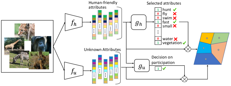
Figure 1: Few-shot classification using our framework. Top: The process of predicting and selecting relevant human-friendly attributes for the current episode. Bottom: The process of predicting unknown attributes and deciding whether the unknown attributes should participate in the current episode or not.

In this paper, we propose an inherently interpretable FSL model by focusing on human-friendly attributes. At the core of the proposed method is interpretability and the ability to trace back decisions to human-friendly attributes. We believe that in many real-world scenarios if a task can be solved along the human-friendly dimensions (attributes), then that should be the preferred way compared to black-box approaches, and equally important is to have a mechanism to detect and deal with novel tasks where the attributes are not adequate. We assume that there exists a large pool of attributes in the same way that we assume there exists a large pool of tasks (base classes) for FSL. The challenges, however, are 1) how to effectively use attributes to do novel tasks in an interpretable way 2) how to know when a novel task cannot be properly done using the available pool of attributes and 3) what to do in such circumstances. We have proposed a solution for each of the three questions. To the best of our knowledge, our work is the first to address these issues in a unified framework. Contributions of this paper are as follows:

1) We propose a mechanism for FSL based on human-friendly attributes. It does not require attribute labels during inference. 2) Not all attributes might be relevant to the task at each episode of few-shot learning. Therefore, we proposed an online attribute selection mechanism that improves interpretability and few-shot classification accuracy by filtering out irrelevant attributes in each episode. 3) We propose a mechanism that detects the episodes where the pool of known attributes are not adequate for the novel task and compensates them by engaging unknown attributes. Unknown attributes are learned to complement the human-friendly attributes without overlapping them by minimizing mutual information during training. This prevents the overlap between human-friendly attributes and unknown attributes from hurting the possibility of human test-time intervention on human-friendly attributes. Figure 1 shows the process of learning and selecting relevant attributes in an episode of 5-way 1-shot setting. Black-box FSL models are more free to concentrate solely on attaining high accuracy. Despite this, the proposed interpretable method performs on par with four previously state-of-the-art black-box FSL models on four widely used datasets.

2 Related Work

Few-shot learning approaches can be roughly grouped into two main categories, optimization-based methods [21, 2] and metric-based approaches [25, 23]. Optimization-based approaches aim at learning a base network that can be adapted to a target task in a few gradient steps [4]. On the other hand, metric-based approaches attempt to learn a unified metric space across different tasks in which each task could be solved using a similarity or distance measure or by using a simple classifier. In this category, MatchingNet [28] utilizes a memory module to effectively leverage the information in each task and performs one-shot classification using cosine metric. ProtoNet [24] learns an embedding space in which the samples of each class could be clustered around the corresponding class-specific prototype. RelationNet [26] attempt to learn a network to measure the similarity between few-shot pairs. The proposed framework lies in the second category and follows ProtoNet. However, unlike this method and all of the above-mentioned approaches that lack interpretability, the decision of our framework can be interpreted by human since it targets attribute space as a human-friendly metric space.

Research in few-shot learning with interpretability in mind has been scarce. There has been several prior work that considered utilizing attention module in representation learning that leads to achieving post-hoc interpretability. RENet [13] employs self-correlation module to extract structural patterns and cross-correlation module to produce co-attention between images. SARN [11] proposes a self-attention relation network that learns non-local information and improves extracted features. Different from the above-mentioned approaches, COMET [4] attempts to propose an intrinsic interpretable FSL model by learning along human interpretable concepts. However, COMET has a number of limitation: it requires concept annotations at pixel-level. It requires such fine-grained annotations not only for base classes but also for test samples. Moreover, it requires all the concepts to be present in each sample and shared among all images. In contrast, our method does not require concept annotations at test time. It requires only concept annotations in the form of binary attributes. Annotations are required only for training classes also known as base classes. Moreover, each attribute can be present or absent in some images. Therefore, it makes our framework applicable to a wider range of scenarios.

Relation to Concept Bottleneck Models: Recently, semantic attributes have been used to learn models that bring the possibility of human interaction and achieve interpretability. Concept Bottleneck Models (CBMs) [15] are the main approaches in this direction that aligns an intermediate layer of a neural network with attributes which subsequently are used to predict the output. The proposed method follows the idea of concept bottleneck models with a focus on extending them to few-shot classification setting since base structure is not compatible with FSL. Moreover, we argue that an interpretation based on all the available attributes may not be advantageous particularly if the number of attributes are high. Also, not all of the attributes are relevant to the task at each episode. Therefore, we propose an attribute selection mechanism to filter out irrelevant attributes in each episode.

Relation to Zero-shot Learning: Zero-Shot Learning (ZSL) utilizes semantic information to compensate unavailability of training instances for unseen classes and serve a bridge to transfer the knowledge from seen classes to unseen ones [32]. Similar to zero-shot learning, we also leverage human-friendly attributes. However, in ZSL attributes are used to account for the lack of training samples in novel classes, rather than interpretibility. Moreover, zero-shot learning uses the attributes for both its training and testing classes to achieve knowledge transferability, but we use attributes just for training classes known as base classes in few-shot learning problem.

Using attribute supervision in Few-shot Learning: Semantic attributes have also been utilized in Few-shot learning. In [27], Tokmakov and et. al employed attributes to improve the compositionality of image representation. Dual TriNet [7] learns an autoencoder framework and leverages semantic attributes to augment visual features for few-shot classification. AGAM [10] learns an attribute-guided attention module to learn more discriminative features by focusing on important channels and regions. Although these methods also leverage semantic information similar to our method, they have used attributes mainly to augment the visual information to achieve higher classification accuracy without any interpretability consideration whatsoever. Although post-hoc saliency approaches can be applied to any of these models, these explanation methods are exposed to the risk of providing unreliable interpretation [1]. This is in contrast to our proposed method where interpretability is at core and the attributes act as bottleneck to ensure decisions can be traced back to human-friendly attributes.

3 Proposed Method

Suppose that we are given a labeled dataset $\mathcal{D}^{b}={\{(x_{i},y_{i})\}}_{i=1}^{N_{b}}$ for base classes $\mathcal{Y}_{b}$ with sufficient images for each class, and a limited number of labeled samples for novel classes $\mathcal{Y}_{n}$ known as support set $\mathcal{S}_{n}={\{(x_{i},y_{i})\}}_{i=1}^{N_{s}}$ where ${\mathcal{Y}_{b}}\cap{\mathcal{Y}_{n}}={\emptyset}$. The goal is to predict the label of a query set $\mathcal{Q}_{n}={\{(x_{i},y_{i})\}}_{i=1}^{N_{q}}$ which also belongs to novel classes ${\mathcal{Y}_{n}}$. It is assumed that each image $x_{i}$ in $\mathcal{D}^{b}$ is associated with a binary attribute vector $a_{i}\in\mathbb{R}^{A}$ that specifies the properties related to the object in the image. These attributes help achieve interpretability.

Our interpretable attribute-based model consists of an attribute predictor $f_{h}$ that attempts to map each image to corresponding human-friendly attribute vector and attribute selector $g_{h}$ that selects the most relevant human-friendly attributes for each episode of few-shot classification. To further improve accuracy, we enable leveraging additional attributes (unknown attributes) by training an unknown attribute predictor $f_{u}$, and an unknown attribute participation detector $g_{u}$ that decides whether unknown attributes should participate in the current episode or not. The process is shown in Fig 1 for a 5-way 1-shot episode. The proposed framework is trained on the images of base classes. Then, it is used to perform few shot classification on novel classes in target space.

3.1 Attribute Predictor Network

In this subsection, we explain the human-friendly attribute predictor network $f_{h}$. This network acts as a feature extractor for few-shot classification. The conventional feature extractors designed for few-shot classification usually just focus on learning some features to achieve a high accuracy, neglecting the interpretability of the learned features and the decision made by using those features. Therefore, we target the attribute space as a meaningful embedding space for few-shot classification and train $f_{h}$ to predict attributes for each image.

The attribute predictor network $f_{h}$ attempts to map each image ${x_{i}}$ to corresponding attribute vector $a_{i}$ by predicting $\hat{a}_{i}$:

$$\hat{a}_{i}=f_{h}(x_{i})$$ (1)

We define the loss function for attribute prediction as a sample-wise weighted binary cross entropy between the actual attribute values and the predicted values:

$$l_{att}=-\sum_{x_{i}\in\mathcal{D}^{b}}\sum_{j=1}^{A}w_{x_{i}}^{j}[a_{x_{i}}^{j}\log{\hat{a}_{x_{i}}^{j}}+(1-a_{x_{i}}^{j})\log{(1-\hat{a}_{x_{i}}^{j})]}$$ (2)

where $w_{x_{i}}^{j}$ is the weight associated with the loss imposed by the $j^{th}$ attribute of image $x_{i}$ and is equal to $1/n_{x_{i}}^{j}$ where $n_{x_{i}}^{j}=|\{a_{x_{i}}^{k}\in a_{x_{i}}|a_{x_{i}}^{k}=a_{x_{i}}^{j}\}|$. Intuitively, $n_{x_{i}}^{j}$ is the number of attributes that are present (absent) in $x_{i}$, if $j^{th}$ attribute is present (absent) in $x_{i}$. Since the majority of the attributes are usually absent (equal to 0) in each image, utilizing standard binary cross entropy results in a bias toward predicting the value of the attributes as 0. Therefore, instead of considering equal weights for different attributes of each sample, the loss value for each present attribute is normalized by the total number attributes that are present in that sample. Likewise, the loss related to the absent attributes are normalized by the total number of absent attributes in that sample. By considering this weighted binary cross entropy, the weight of the minority class is increased.

After training on the images of base classes using $l_{att}$ in Eq. 2, the attribute predictor network can be used to predict the attributes of novel images and perform few-shot classification in attribute space. A class-specific prototype $c$ is calculated in the attribute space for each class $y$ by averaging the attributes of the support set:

$$\hat{c}_{y}=\frac{1}{|S_{y}|}\sum\limits_{x_{i}\in{S_{y}}}\hat{a}_{x_{i}}$$ (3)

where $|S_{y}|$ is the number of images in the support set of the class $y$. To specify the class of a query image $x_{q}$, the distance of its predicted attributes $\hat{a_{x_{q}}}$ is calculated from the class-specific prototypes. This distance is used to measure the probability of the query image belonging to each class. Therefore, the probability of assigning the query image $x_{q}$ to the class $y$ is estimated as:

$$p(y|x_{q})=\frac{exp(-d(\hat{a}_{x_{q}},\hat{c}_{y}))}{\sum_{y^{\prime}\in{\mathcal{Y}_{s}}}exp(-d(\hat{a}_{x_{q}},\hat{c}_{y^{\prime}}))}$$ (4)

where $d(.)$ is a distance function.

Although the probability of assigning an image to one class can be interpreted in terms of the difference between the predicted attributes of query image and the prototypes of novel classes, in fact this interpretation may not be advantageous since the number of attributes is usually high. Moreover, some attributes may not be relevant to the classes of individual episodes of few-shot classification. Therefore, employing all attributes may degrade the classification accuracy.

To tackle the above problems, an attribute selector network is proposed in the next sub-section that will be employed to select relevant attributes in each episode of few-shot recognition.

3.2 Attribute Selector Network

After training the attribute predictor network $f_{h}$, the weights of $f_{h}$ are frozen and a selector network $g_{h}$ is trained to select useful attributes for few-shot classification. To mimic few-shot recognition tasks during training of this network, the images of base classes are sampled in the form of episodes. In each episode, N classes are randomly selected from the base classes. For each of these classes, a support set $\mathcal{S}_{b}$ consists of K instances and another subset serving as the query set $\mathcal{Q}_{b}$ are sampled.

The attribute predictor network exploits the attributes of the support set to select relevant attributes for classification of the query set. The presence or absence of each attribute is modeled by a categorical distribution with two possible values of either 0 or 1. Therefore, the number of categorical distributions will be equal to the number of attributes. In each episode, by sampling from these categorical distributions, a binary state vector is obtained which determines which attributes should be used in that episode.

In each episode, the attribute vectors for the support set of each class are averaged to obtain the prototype of each class. Then, these prototypes are fed to $g_{h}$ that consists of a Bi-LSTM followed by a feed-forward network. The Bi-LSTM will effectively aggregate the information from the attribute prototypes of all classes and provides unified features for them. The last hidden state of the forward and backward LSTMs are concatenated and passed through a feed-forward network with sigmoid activation function in the final layer to produce the probabilities of the Bernoulli categorical distributions. The output is a vector with a dimension equal to the number of attributes where the $i^{th}$ element denoted as $\pi_{i}$, represents the probability of the $i^{th}$ attribute being selected. Clearly, the probability of the same attribute being disregarded is $1-\pi_{i}$.

While the output for the binary-trial of each categorical distribution can be determined by sampling, it is a non-differentiable operation. To tackle this problem, we use Gumbel Softmax estimator [12, 17] that enables a differentiable sampling process from categorical distributions using reparameterization trick [14, 20]. Therefore, the output value that specifies whether the $i^{th}$ attribute is selected or not is determined as:

$$s^{(i)}=\\ \frac{\exp{((\log\pi_{i}+\gamma_{i})/\tau)}}{\exp{((\log\pi_{i}+\gamma_{i})/\tau)}+\exp{((\log\pi_{i^{\prime}}+\gamma_{i^{\prime}})/\tau)}}$$ (5)

where $\pi_{i^{\prime}}$ = $1-\pi_{i}$, $\gamma_{i}$ and $\gamma_{i^{\prime}}$ are two Gumbel noises sampled from standard Gumbel distribution. Furthermore, $\tau$ is a temperature parameter determining the degree of discreteness. When $\tau\rightarrow 0$, the output becomes discrete. During training, we use Gumbel Softmax estimator to specify the states of embedding spaces (i.e. selected attributes). During inference, we simply select the binary value with higher probability as the state of each embedding space (i.e. no Gumbel Softmax sampling).

The state vector $s$ is used as the weight vector to scale the dimensions of the attribute space. Therefore, following Eq. 4, the probability of assigning the query image $x_{q}$ to the class $y$ is estimated as

$$p(y|x_{q})=\frac{exp(-d(s\odot{\hat{a}_{x_{q}}},s\odot{\hat{c}_{y}}))}{\sum_{y^{\prime}\in{\mathcal{Y}_{s}}}exp(-d(s\odot{\hat{a}_{x_{q}}},s\odot{\hat{c}_{y^{\prime}}}))}$$ (6)

where $\odot{}$ denotes the element-wise product operation. When $s_{i}$ is 1, the $i^{th}$ attribute is active and the distance along the corresponding dimension will affect the class membership probabilities calculated in the episode. Similarly when the state is 0, the attribute will not influence the classification. Therefore, only the relevant attributes selected in each episode are used in the classification.

The loss term for few-shot classification to train $g_{h}$ is formulated as:

$$l_{cls}=-\sum_{x_{q}\in\mathcal{Q}_{b}}\log p(y_{x_{q}}|x_{q})$$ (7)

The probabilities used in $l_{cls}$ are computed using Eq. 6. Although the attribute selection mechanism can improve interpretability by decreasing the number of attributes participating in the few-shot recognition, this reduction is not guaranteed. Therefore, we also use $l_{1}$ norm of the binary states vector $s$ to further control and reduce the number of selected attributes in each episode. The final objective function to train $g_{h}$ is:

$$l_{sel}=\alpha l_{cls}+\eta l_{1}$$ (8)

where the hyperparameters $\alpha$ and $\eta$ specify the weights of the loss terms.

3.3 Unknown Attribute Participation

Human-friendly attributes may not always be able to properly perform few-shot learning due to their insufficiency and lack of quality. To address such situations and close the performance gap, we propose a method that allows trading interpretability for accuracy. We aim to improve accuracy by introducing unknown attributes $\bar{a}$ to be used additional to the human-friendly attributes for few-shot classification. The new attributes are called unknown since they are not human-friendly; we learn them during training.

In each episode, we attempt to balance the interpretability and accuracy by automatically deciding whether the unknown attributes should be involved or not. This is achieved by training a network $g_{u}$ that receives the human-friendly and unknown attributes and makes the above decision. $g_{u}$ aims to detect when the human-friendly attributes are not adequate and adding unknown attributes would be most effective.

To learn unknown attributes suitable for few-shot classification, we train a network $f_{u}$ with the same structure as $f_{h}$ using the objective function $l_{cls}$ shown in Eq. 7 . The probability in Eq. 7 is calculated by Eq. 4. The trained network $f_{u}$ is then used to extract embedding features acting as unknown attributes for each sample.

Although training $f_{u}$ using $l_{cls}$ can results in obtaining unknown attributes suitable for few-shot classification, they may have some overlap with human-friendly attributes. This overlap hurts the possibility of human test-time intervention on human-friendly attributes. Therefore, we also consider minimizing the mutual information I between the learned human-friendly attributes $\hat{a}$ and unknown attributes $\bar{a}$ during training $f_{u}$:

$$\min_{f_{u}}I(\bar{a},\hat{a})$$ (9)

However, due to unavailability of a direct general-purpose procedure for optimizing the above problem in a high dimensional space, we leverage the mutual information neural estimator presented in [3] and consider the following minimax problem:

$$l_{MI}=\min_{f_{u}}\max_{f_{I}}\mathbb{E}[f_{I}(\bar{a},\hat{a})]-log(\mathbb{E}[exp(f_{I}(\bar{a},\hat{a}))])$$ (10)

where $f_{I}$ is an auxiliary network used to estimate the mutual information by solving the interior maximization problem. The final objective function to train the $f_{u}$ is:

$$l_{fake}=l_{cls}+\lambda l_{MI}$$ (11)

where $\lambda$ controls the mutual information minimization term. The total number of unknown attributes is the same as the total number of human-friendly attributes.

Table 1: Results on CUB and aPY with 5-way setting. Mean accuracy with 95% confidence interval over 600 episodes sampled from novel classes is reported.

Method CUB aPY 1-shot 3-shot 5-shot 1-shot 3-shot 5-shot MatchingNet 60.3 $\pm$ 1 71.0 $\pm$ 0.8 74.2 $\pm$ 0.6 40.6 $\pm$ 0.7 53.3 $\pm$ 0.7 56.1 $\pm$ 0.7 MAML 55.6 $\pm$ 1 63.4 $\pm$ 0.9 66.4 $\pm$ 0.8 40.7 $\pm$ 0.7 48.2 $\pm$ 0.7 49.4 $\pm$ 0.6 RelationNet 60.3 $\pm$ 0.9 69.0 $\pm$ 0.7 72.1 $\pm$ 0.7 38.1 $\pm$ 0.7 46.7 $\pm$ 0.6 52.3 $\pm$ 0.7 ProtoNet 53.8 $\pm$ 0.9 67.1 $\pm$ 0.7 71.4 $\pm$ 0.8 41.9 $\pm$ 0.8 51.0 $\pm$ 0.7 56 $\pm$ 0.7 Ours 56.3 $\pm$ 0.9 66.7 $\pm$ 0.8 71.4 $\pm$ 0.8 40.6 $\pm$ 0.7 46.9 $\pm$ 0.7 53.5 $\pm$ 0.7

The final loss function for the proposed model with $g_{u}$ is similar to Eq. 8 where $l_{1}$ is the output of $g_{u}$ and $\beta$ is the corresponding hyper-parameter. Moreover, $l_{cls}$ is calculated in the mixed space of unknown attributes and human-friendly attributes. The human-friendly attributes and unknown attributes are concatenated to construct this mixed space. For each sample, the output value of $g_{u}$, which is a scalar, is used as the weight for each of the unknown attributes and the binary weight vector returned by $g_{h}$ is used to weight the human-friendly attributes. Detailed explanations on training $g_{u}$ as well as achieving unknown attributes are provided in supplementary materials. It is noteworthy that the recent few-shot learning methods including MetaBaseline [6] and NegMargin [16] can be adapted to achieve unknown attributes. We leave this for future work.

4 Experiments and Evaluation

Table 2: Results on SUN and AWA with 5-way setting. Mean accuracy with 95% confidence interval over 600 episodes sampled from novel classes are reported.

Method SUN AWA 1-shot 3-shot 5-shot 1-shot 3-shot 5-shot MatchingNet 63.2 $\pm$ 1 74.1 $\pm$ 0.8 78.3 $\pm$ 0.8 45.1 $\pm$ 0.9 54.4 $\pm$ 0.7 59.9 $\pm$ 0.7 MAML 60.6 $\pm$ 1 68.6 $\pm$ 0.9 70.3 $\pm$ 0.9 35.1 $\pm$ 0.8 44.1 $\pm$ 0.8 46.9 $\pm$ 0.7 RelationNet 62.9 $\pm$ 0.9 72.7 $\pm$ 0.8 77.7 $\pm$ 0.8 44.6 $\pm$ 0.8 52.9 $\pm$ 0.7 56.1 $\pm$ 0.7 ProtoNet 63.7 $\pm$ 0.9 75.6 $\pm$ 0.7 78.6 $\pm$ 0.7 44.5 $\pm$ 0.8 53.3 $\pm$ 0.8 59.1 $\pm$ 0.7 Ours 61.4 $\pm$ 1 72.2 $\pm$ 0.9 76.5 $\pm$ 0.7 42.6 $\pm$ 0.7 51.5 $\pm$ 0.8 56.1 $\pm$ 0.7

In this section, we first describe the datasets, experimental settings and implementation details. Then we present the results of the proposed interpretable method and compare it with a number of previously state-of-the-art black-box FSL methods.

4.1 Experimental Setup

Datasets and experimental settings: We conduct experiments on four popular computer vision datasets with available attributes including Caltech-UCSD Birds-200-2011 (CUB) [29], Animals with Attributes (AWA) [30], SUN Attributes (SUN) [19] and Attribute Pascal and Yahoo (aPY) [8]. The statistics of these datasets and their setup are provided in supplementary materials.

The experiments are performed on three widely used 5-way 1-shot, 5-way 3-shot and 5-way 5-shot settings. For each class, a query set consists of 16 samples is constructed in each episode for CUB, AWA and aPY. For SUN, the query set contains 10 samples due the lower number of instances in each class. In each experiment, we report the mean accuracy with 95% confidence interval over 600 episodes sampled from novel classes which is widely used as performance measure of FSL approaches.

Implementation Details: As the attribute predictor network, we use a four blocks convolutional neural network similar to Conv-4 [23] which is one of the most adopted backbone networks for FSL. In the original network, each block consists of a 3 × 3 convolution with 64 filters, followed by a batch normalization layer, a Relu non-linearity and a 2 × 2 max pooling layer. However, we change the number of filters to achieve feature maps with the number of channels equal to the total number of attributes in the final block. The Conv-4 is followed by a global average pooling. Then the features are fed to a linear layer with tanh activation function for its more symmetric properties and a wider output range compared to sigmoid activation function. The output is then normalized to have a range of [0,1], compatible with binary cross entropy. The attribute selector network consists of a one layer Bi-LSTM with 100 features in the hidden state, followed by a one-layer perceptron with sigmoid activation function. The Gumbel softmax sampler then uses the output of the selector network. In all experiments, $\alpha$ is set to 1 and the value of $\eta$ is specified in each subsection. More details regarding our implementation are available in supplementary materials.

4.2 Performance comparison

As discussed previously, attributes act as bottleneck in our method to ensure decisions can be traced back to human-friendly attributes. We seek to maximize the accuracy but within the interpretability constraint mentioned above. For the above reason, it is not expected that the proposed method always outperforms black-box methods and we do not claim that an interpretable method should necessarily beat black-box models. Despite this, the proposed method achieved results that are competitive with the previously state-of-the-art FSL methods including MatchingNet [28], MAML [9], RelationNet [26] and ProtoNet [24]. Arguably, these are seminal works in the area of FSL. The results are presented in Tables 1 and 2. To have a fair comparison, all the methods are implemented using the same backbone network. Note that we did not use unknown attributes in this experiment. Moreover, the L1 norm is not applied on the output of $g_{h}$ (i.e. $\eta=0$).

We evaluate the effectiveness of the attribute selector in the next subsection and provide the attribute predictor network performance evaluation in supplementary materials.

4.3 Attribute selector evaluation

The attribute selector network aims to select a subset of the most relevant attributes in each few-shot episode. In this section, we examine the effectiveness of the attribute selector network by comparing it with a base model that does not do attribute selection. Similar to the previous section, we do not leverage unknown attributes in this experiment. The base model consists of just $f_{h}$ and performs few-shot learning using Eq. 4. Therefore, all attributes participate in few-shot classification. The results of these experiments are presented in the first column of Tables 3, 4, 5, 6. We also examine the effect of the ($l_{1}$) loss by examining different values of $\eta$ selected from the values [$0$,$10^{-5}$, $10^{-4}$, $10^{-3}$]. $\eta=0$ correspond to the proposed model without the ($l_{1}$) loss. We provided the average number of selected attributes in addition to the mean accuracy. Compared to the baseline model, the proposed method has reduced the number of attributes by 48, 38.4, 27.4 and 42% while improving the accuracy by an average of 2.8, 1.8, 1.2 and 0.4% on CUB, aPY, SUN and AWA datasets, respectively. Increasing $\eta$ significantly reduces the average number of selected attributes at the cost of only a slight drop in accuracy. For example, increasing $\eta$ from 0 to $10^{-3}$ reduces the average number of selected attributes by 62, 23, 33, and 33% on CUB, aPY, SUN and AWA datasets, respectively, while hindering the accuracy by only 1.17, 1.14 , 0.5%, and in the case of AWA the accuracy actually improved by 0.66%. Furthermore, the number of selected attributes decreases when the size of the support set is reduced from K=5 to 1. This is an interesting behavior that demonstrates how the proposed method attempts to avoid the overfitting problem by choosing fewer attributes. We provide qualitative examples regarding attribute selection mechanism in supplementary materials.

Table 3: Evaluating the impact of attribute selector network on CUB in terms of average accuracy and number of attributes. The base model does not have $g_{h}$. The total number of attributes is 312 for this dataset.

Setting Base $\eta$ $0$ $10^{-5}$ $10^{-4}$ $10^{-3}$ 1-shot Acc 52.4 56.3 56.6 55.9 55 # Att 312 97.1 93.5 80.6 44.1 3-shot Acc 64.1 66.7 66.8 66.3 65.7 # Att 312 170.6 154.7 133.4 67.1 5-shot Acc 69.5 71.4 71.4 73.5 70.2 # Att 312 219.1 186.5 148.9 73

Table 4: Evaluating the impact of attribute selector network on aPY in terms of average accuracy and number of attributes. The base model does not have $g_{h}$. The total number of attributes is 64 for this dataset.

Setting Base $\eta$ $0$ $10^{-5}$ $10^{-4}$ $10^{-3}$ 1-shot Acc 40.0 40.6 40.8 40.8 39.9 # Att 64 36.4 34.2 30 25.8 3-shot Acc 45.2 46.9 46.4 46.3 46 # Att 64 38.5 37.5 34.1 32.6 5-shot Acc 50.3 53.5 52 52 51.7 # Att 64 43.4 39.1 35.9 33

Table 5: Evaluating the impact of attribute selector network on SUN in terms of average accuracy and number of attributes. The base model does not have $g_{h}$. The total number of attributes is 102 for this dataset.

Setting Base $\eta$ $0$ $10^{-5}$ $10^{-4}$ $10^{-3}$ 1-shot Acc 60.4 61.4 59.6 60.3 60.3 # Att 102 53.48 50.7 50.4 38.4 3-shot Acc 72.0 72.2 72.8 72.9 72.3 # Att 102 82.4 80.7 77 51.9 5-shot Acc 74.1 76.5 76 75.4 76 # Att 102 86.2 83.9 81.2 58

Table 6: Evaluating the impact of attribute selector network on AWA in terms of average accuracy and number of attributes. The base model does not have $g_{h}$. The total number of attributes is 85 for this dataset.

Setting Base $\eta$ $0$ $10^{-5}$ $10^{-4}$ $10^{-3}$ 1-shot Acc 41.8 42.6 42.6 43.5 42.7 # Att 85 39.8 38.7 38.2 29.5 3-shot Acc 51.8 51.5 52.3 51.2 53.3 # Att 85 52.3 51.9 46.7 35.3 5-shot Acc 55.3 56.1 55.9 56 56.2 # Att 85 55.7 50.7 48.1 34

Table 7: Evaluating the effectiveness of the proposed $g_{u}$ on AWA and CUB datasets in 5-way 1-shot setting.

Dataset CUB10% CUB AWA10% AWA $\beta$ 1.75 1.7 - 0.7 0.8 - 0.3 0.4 - 0.03 0.04 - % of human-friendly episodes 28.3 74.8 100 50.3 84 100 35.5 69.3 100 48 89.3 100 Accuracy with $g_{u}$ 58.6 52 48.1 60.5 57.5 56.3 40.8 38.3 36.3 45.2 43.1 42.6

4.4 Closing the Accuracy Gap

Looking at Table 1 and 2, it can be seen that among the four datasets, the biggest performance gap between the proposed method and the bests black-box method is on CUB and AWA. This could be because the attributes or their quality are not adequate to distinguish the classes. In this section, we provide the results of incorporating unknown attributes as disused in Section 3.3.

The results of this experiment on CUB and AWA in 5-way 1-shot setting are shown in Table 7. To further evaluate how well the proposed approach can compensate for accuracy when the attributes are incomplete, we also report the results on two new versions of CUB and AWA with only 10% of the attributes randomly selected, namely CUB10% and AWA10%, respectively. $\beta$ controls the proportion of human-friendly episodes among all 600 sampled episodes of novel classes. We report the results of the models trained with two different values of $\beta$ on each dataset. We consider $\{1.7,1.75\}$, $\{0.7,0.8\}$, $\{0.3,0.4\}$ and $\{0.03,0.04\}$ for CUB10%, CUB, AWA10% and AWA, respectively.

On the AWA dataset, by using $g_{u}$ we were able to get closer to the accuracy of the best black-box model (45.1%) by improving the accuracy from 42.6 to 43.1, and yet making interpretable decisions in 89.3% of the episodes. For a smaller value of $\beta$, the proposed approach surpassed the best model by achieving an accuracy of 45.2% while 48% episodes still were handled by only human-friendly attributes. On the CUB dataset, we were able to improve the accuracy from 56.3 to 60.5 and consequently not only close the gap but also outperform the best black-box model while making interpretable decisions in more than half of the episodes. Finally, it can be seen that the accuracy promotion by utilizing unknown attributes is more significant when the number of human friendly attributes is decreased to 10% in AWA10% and CUB10% datasets.

4.5 Preferability of human-friendly attributes over unknown attributes

As seen in the previous subsection, the performance of the framework can be improved by utilizing unknown attributes when the known attributes are incomplete. Even in the episodes that the model leverages unknown attributes, the entire package is still interpretable since unknown attributes can be explained using saliency methods such as Grad-CAM [22]. Examples of Grad-Cam visualization for different unknown attributes of CUB and AWA datasets are provided in supplementary materials. Interestingly, the unknown attributes desire visually fine-grained attributes including body parts that can very well complement abstract known attributes.

Although the utilized saliency explanation can reveal useful information about what the model has focused on for the final decision, there is no guarantee regarding the reliability of the explanation [1] and sometimes they can be misleading. This is a limitation of such approaches; it is not a phenomenon specific to our unknown attribute learning paradigm. Therefore, all the black-box models that utilize similar post-hoc interpretability approaches are facing the same challenge. Even if we assume this kind of explanation is reliable, it is often difficult to interpret the explanation in the direction of the model’s decision, especially for fine-grained classification tasks. For example, Figure 2 shows the Grad-CAM of an unknown attribute for a support set and a query sample on the CUB dataset. Although saliancy maps provide spacial localization, it is not apparent what exactly the model has focused on in that region; is it beak shape, beak color, eye color? On the other hand, the proposed method was able to successfully recognize the human-friendly attributes that are useful for classification of the query sample including white eye, black forehead, and black crown. This highlights the advantages of the proposed method over attempting to produce post-hoc explanations for a black-box model.

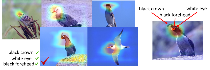
Figure 2: The Grad-cam visualization of an unknown attribute for a support set (left) and a query example (right) on CUB dataset. While heatmaps provide spacial localisation, they fail to indicate what exactly the model has focused on in a region. Is it beak shape, beak color, eye color? The human-friendly attributes detected by the proposed method can very well address this shortcoming.

4.6 Human Intervention

In this subsection, we consider the capability of our framework in enabling interaction with human by performing intervention on misclassified query samples. We report the performance on AWA and CUB datasets in 5-way 1-shot setting with respect to intervening 5% and 10% of human-friendly attributes selected by $g_{h}$ in each episode. We consider intervention on the framework performing in joint attributes space (With unknown attributes) and when only human-friendly attributes are used (Without unknown attributes). Note that in this experiment, there is no real-world human interaction. Instead, we rely on ground-truth annotations to simulate intervention and assume that real-world human intervention would be consistent with the ground-truth annotations. In summary, the intervention improved the performance in all settings, obtaining an average improvement of 2.8% and 2.65% on CUB and AWA, respectively. The promotion was more significant with a higher ratio of intervention ($10\%$) in all cases and in human-friendly attribute space compared to joint attribute space. More details of the intervention process and the complete results are provided in supplementary materials.

5 Conclusion

In this paper, we proposed an inherently interpretable few-shot learning method based on human-friendly attributes. During inference, the proposed method does not need the attributes. Attributes are extracted from input. Moreover, an attribute selection mechanism was proposed to filter out irrelevant attributes in each few-shot learning episode which in turn improves the accuracy. The proposed interpretable method achieved results on par with the previously state-of-the-art black-box few-shot learning methods. We also proposed a method that aimed to close the accuracy gap with the black-box models by automatically detecting the episodes that can benefit the most from unknown learned attributes. We demonstrated that this approach is effective in closing the performance gap while delivering interpretable FSL classification in a substantial number of episodes.

Appendix A Appendix

A.1 Datasets and Settings Description

CUB is a fine-grained dataset containing 11,768 images from 200 bird classes. For each image, 312 binary attributes are provided in this dataset. Following the protocol proposed by [5], we divide the dataset into the same 100 base classes, 50 validation and 50 novel classes. AWA consists of 37,322 animal images from 50 different categories, with 85-dimensional class-level attribute vectors. We use the first 30 categories as base classes, the next 10 classes as validation and the last 10 categories as novel classes. SUN is a fine-grained scene dataset with 14340 images from 717 different classes. Each image is provided with 102 attribute. For each attribute, a continuous value in range of [0,1] is calculated by averaging the votes of three annotators. We round each value to achieve binary attributes. Furthermore, we divide this dataset into 580 base classes, 65 validation and 72 novel classes. aPY is a course-grained dataset containing 15,339 images from 32 classes, 20 Pascal and 12 Yahoo classes. All Yahoo classes are used as novel ones and 15 Pascal classes are used as base classes. The remaining 5 Pascal classes are used as validation categories. Each image in this dataset is provided with 64 attributes.

A.2 Additional Implementation Details

We apply data augmentation including color jittering and random horizontal flipping. Furthermore, the input size of 84 × 84 is used for all datasets. Both attribute predictor network and attribute selector network are trained using Adam optimizer with a learning rate equal to $10^{-3}$.

The attribute predictor network $f_{h}$ is trained for 100 epochs with mini batch size of 128 on all datasets. After each epoch, the attribute prediction performance on the samples of validation classes is measured. Then, the model with the best performance on validation classes is selected as the final network.

The attribute selector network $g_{h}$ is trained for 200,000 episodes, evaluated on 600 sampled episodes of validation classes every 500 episodes. The model achieving the best performance on the validation episodes will be the final network. The temperature parameter of Gumbel Softmax estimator ($\tau$) in $g_{h}$ is initialized to 4, halved every 12500 episodes during training until reaching to 0.5.

We set $\alpha$ equal to 1 in all experiments. Since there are just two hyper-parameters in the objective function of Eq. 8, we keep $\alpha$ fixed and change the other ($\gamma$) to tune the impact of their corresponding loss terms in the objective function. Moreover, we report the results of our framework with various values of $\gamma$ selected from [$0$,$10^{-5}$, $10^{-4}$, $10^{-3}$]. These numbers are picked to cover a wide range of reduction rate in the average percentage of participated attributes in episodes and selected based on the performance of the framework on validation classes.

Input: $f_{u}$ and $f_{I}$ with their initialized weights $\theta_{f_{u}}$ and $\theta_{f_{I}}$, trained $f_{h}$

for $E_{1}$ episodes do

       Draw $N$ samples ($S$) from $N_{b}$

       Obtain human-friendly attributes for $S$ using $f_{h}$: $\hat{A}_{S}=\{\hat{a}_{x}|x\in S\}$

       Obtain unknown attributes for $S$ using $f_{u}$: $\bar{A}_{S}=\{\bar{a}_{x}|x\in S\}$

      

      for $E_{2}$ episodes do

             Draw $N$ samples ($S^{\prime}$) from $N_{b}$

             Obtain unknown attributes for $S^{\prime}$ using $f_{u}$: $\bar{A}_{S^{\prime}}=\{\bar{a}_{x}|x\in S^{\prime}\}$

             Calculate the lower-bound: $l_{MI}(\theta_{f_{I}})=\frac{1}{N}\sum_{i=1}^{N}f_{I}({\bar{A}_{S}}^{i},{\hat{A}_{S}}^{i})-\log(\frac{1}{N}\sum_{i=1}^{N}e^{f_{I}({\bar{A}_{S^{\prime}}}^{i},{\hat{A}_{S}}^{i})})$

             Update $\theta_{f_{I}}$ using $Adam(-l_{MI}(\theta_{f_{I}}))$

            

       end for

      

      Draw $N$ samples ($S^{\prime\prime}$) from $N_{b}$

       Obtain unknown attributes for $S^{\prime\prime}$ using $f_{u}$: $\bar{A}_{S^{\prime\prime}}=\{\bar{a}_{x}|x\in S^{\prime\prime\}}$

       Calculate loss: $l_{MI}(\theta_{f_{u}})=\frac{1}{N}\sum_{i=1}^{N}f_{I}({\bar{A}_{S}}^{i},{\hat{A}_{S}}^{i})-\log(\frac{1}{N}\sum_{i=1}^{N}e^{f_{I}({\bar{A}_{S^{\prime\prime}}}^{i},{\hat{A}_{S}}^{i})})$

       Update $\theta_{f_{u}}$ using $Adam(l_{cls}+\lambda l_{MI}(\theta_{f_{u}}))$

      

end for

Algorithm 1 Training $f_{u}$ to learn unknown attributes

A.3 Details of Learning Unknown Attributes and Training $g_{u}$

To learn unknown attributes for classes, we use the same structure as $f_{h}$ for $f_{u}$. $f_{I}$ is an MLP with two hidden layers, both with a dimension of 50 and ReLU activation function. The input is the concatenation of human-friendly attributes and the output of $f_{u}$ that is used as unknown attributes, and the output is the estimated mutual information. The networks $f_{u}$ and $f_{I}$ are trained simultaneously using the algorithm shown in Algorithm 1. In this algorithm, $E_{1}$ and $E_{2}$ are set to 200,000 and 10, respectively. Furthermore, $\lambda$ is to 2. The network is trained using Adam optimizer with a learning rate equal to $10^{-2}$, evaluated on 600 episodes sampled from validation classes every 500 episodes. The network with highest performance on validation episodes is used to extract embedding features acting as unknown attributes for each sample. Examples of Grad-Cam visualization for different unknown attributes of CUB and AWA datasets are shown in Fig 3.

To train $g_{u}$, the weights of our trained framework including $f_{h}$ and $g_{h}$ as well as $f_{u}$ are frozen and we just train $g_{u}$ which has a structure similar to the attribute selector network $g_{h}$ with the difference that this network will decide on the participation of the unknown attributes in each episode. Therefore, its output will be a scalar value. Similar to $g_{h}$, the input of $g_{u}$ is the prototypes of all classes participated in current episode with the difference that each prototype is calculated in the mixed space of unknown attributes and human-friendly attributes.

For each sample, the human-friendly attributes and unknown attributes are stacked to construct this mixed space. Then, the binary weight vector returned by $g_{h}$ is used as the weights of human-friendly attributes. Similarly, the output scalar value of $g_{u}$ is used as the weight for each of the unknown attributes.

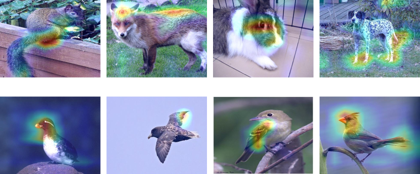
Figure 3: The Grad-cam visualization of four different unknown attributes on AWA dataset (top) and CUB dataset (bottom).

A.4 Attribute predictor network performance

In this section, we evaluate the accuracy of the attribute predictor network. For each sample, the predicted attribute vector $s$ is compared with the ground-truth and an attribute accuracy is calculated for each sample. The mean and standard deviation of the attribute accuracy of individual samples in novel classes are reported in the last column of Table 8. Since the number of attributes present in each sample is usually much less than the number of absent attributes, we also report the mean accuracy of predicting present and absent attributes separately to assure that the model is not biased toward predicting the absence of the attributes due to the imbalanced nature of the attributes. The results are reported in the first two column of Table 8. The results shows that the resulting models perform fairly well on predicting both present and absent attributes which demonstrates the effectiveness of the sample-wise weighted loss function in Eq. 2. Using the original CE loss instead of the sample-wise weighted loss function, almost all attributes were predicted as 0 (i.e. absent). For the aPY dataset, there is a 20% gap between the accuracy of predicting absent and present attributes. This can be due to the weak relation between the base classes and novel classes in aPY so that the model has not been able to effectively transfer the knowledge learned on predicting present attributes of base classes to novel classes. In aPY, base classes are from Pascal and novel classes are from Yahoo classes as described in supplementary materials.

On average, the attribute predictor network is around 80% accurate. This results demonstrates that less than perfect attribute predictors when incorporated into the proposed FSL method, can provide competitive FSL results. This can be attributed to the better generalization of higher level attributes to novel classes which is previously reported in [4] too.

Table 8: Performance of $f_{h}$ in predicting attributes of novel classes. The mean and standard deviation of the attribute prediction accuracy are reported. The accuracy of predicting absent attributes (AB), present attributes (PR) and the overall accuracy (OV) are reported separately.

Dataset	AB	PR	OV
CUB	76.7 $\pm$ 0.7	78.8 $\pm$ 1.5	76.9 $\pm$ 0.7
aPY	85.9 $\pm$ 0.6	62.2 $\pm$ 2.4	82.9 $\pm$ 0.6
SUN	85.2 $\pm$ 0.5	80.1 $\pm$ 1.9	84.9 $\pm$ 0.4
AWA	77.4 $\pm$ 0.6	71.4 $\pm$ 1.1	74.9 $\pm$ 0.7

A.5 Quality of the selected attributes using the online attribute selection mechanism

In Fig 4, we have shown the attributes selected in two real episodes with 5-way 1-shot setting on AWA dataset. In this experiment, to better evaluate the quality of the selected attributes, we have increased the loss term $l_{1}$ and set its weight to 0.01. It can be seen that the selected attributes very well relevant and address the differences between images, implying the effectiveness of the online attribute selection mechanism.

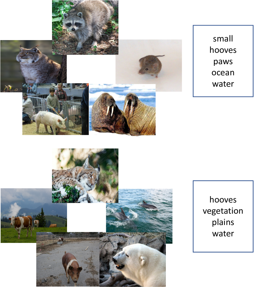
Figure 4: Qualitative examples: The attributes selected by online attribute selection mechanism for two 5-way 1-shot episodes on AWA dataset when $\gamma=0.01$. The selected attributes very well address the differences between images.

A.6 Human Intervention

In conventional concept bottleneck models (CBM), a human can interact with the model by identifying incorrect predicted concepts for miclassified instances and rectify them to see how the final decision will change. This type of intervention is appropriate for CBM since it employs a parametric model for classification on top of the concept bottleneck layer. However, since our model uses a non-parametric approach in its classification phase and its decision also relies on the predicted concepts of the model for other instances (support set), correcting the concept prediction just for the query sample can not reflect the actual effect of the concept in updating final decision. Therefore, we design and present a new form of intervention applicable to our FSL model.

To intervene an arbitrary attribute of a misclassified query instance, the user will observe this sample and the prototypes of different classes in the current episode and decides on the prototype most similar to the query instance in terms of the selected attribute. Then, the query will be moved toward the prototype but only along the dimension corresponding to the attribute in decision space. Since the decision space is the same as the attribute space in our model, the user rectifies the predicted distance between query instance and the prototypes in terms of the attribute that is being intervened.

There is no real-world human interaction in this experience. Instead, we rely on ground-truth annotations to simulate intervention and assume that real-world human intervention would be consistent with the ground-truth annotations. Therefore, to rectify the distance between a misclassified query sample and the prototypes, the prototype with the ground-truth attribute value same as the query sample is identified and the query sample is moved toward this prototype by setting its attribute value equal to the predicted attribute value for the identified prototype in the decision space. If there is more than one prototype with the same ground-truth attribute value, the predictions for all of them are averaged and will be used as the attribute value of the query sample.

We do intervention on the framework performing in joint attributes space (with unknown attributes) and when only human-friendly attributes are used (without unknown attributes). 600 episodes are sampled from novel classes and average accuracy before and after intervention with two intervention ratio (5% and 10%) are reported. It should be noted that in this experiment, unknown attributes are employed in all 600 episodes when evaluating intervention in joint attributes space. The results of this experiment are presented in Table 9.

Table 9: Intervention on AWA and CUB in 5-way 1-shot setting. We report the performance with respect to intervening 5% ($r=5\%$) and 10% ($r=10\%$) of human-friendly attributes selected by $g_{h}$ in each episode. Intervention is performed on misclassified query samples. The performance of the model without any intervention ($r=0\%$) for each setting is also reported for comparison.

Setting CUB AWA $r=0\%$ $r=5\%$ $r=10\%$ $r=0\%$ $r=5\%$ $r=10\%$ With unknown attributes 63.9 65.6 66.7 46.4 47.8 48.9 Without unknown attributes 56.3 59 60.3 42.6 45.2 46.7

References

- [1] Julius Adebayo, Justin Gilmer, Michael Muelly, Ian Goodfellow, Moritz Hardt, and Been Kim. Sanity checks for saliency maps. Advances in neural information processing systems, 31, 2018.
- [2] Antreas Antoniou, Harrison Edwards, and Amos Storkey. How to train your MAML. In International Conference on Learning Representations, 2019.
- [3] Mohamed Ishmael Belghazi, Aristide Baratin, Sai Rajeshwar, Sherjil Ozair, Yoshua Bengio, Aaron Courville, and Devon Hjelm. Mutual information neural estimation. In Jennifer Dy and Andreas Krause, editors, Proceedings of the 35th International Conference on Machine Learning, volume 80 of Proceedings of Machine Learning Research, pages 531–540. PMLR, 10–15 Jul 2018.
- [4] Kaidi Cao, Maria Brbic, and Jure Leskovec. Concept learners for few-shot learning. In International Conference on Learning Representations, 2021.
- [5] Wei-Yu Chen, Yen-Cheng Liu, Zsolt Kira, Yu-Chiang Frank Wang, and Jia-Bin Huang. A closer look at few-shot classification. In International Conference on Learning Representations, 2019.
- [6] Yinbo Chen, Zhuang Liu, Huijuan Xu, Trevor Darrell, and Xiaolong Wang. Meta-baseline: Exploring simple meta-learning for few-shot learning. In Proceedings of the IEEE/CVF International Conference on Computer Vision, pages 9062–9071, 2021.
- [7] Zitian Chen, Yanwei Fu, Yinda Zhang, Yu-Gang Jiang, Xiangyang Xue, and Leonid Sigal. Multi-level semantic feature augmentation for one-shot learning. IEEE Transactions on Image Processing, 28(9):4594–4605, 2019.
- [8] Ali Farhadi, Ian Endres, Derek Hoiem, and David Forsyth. Describing objects by their attributes. In 2009 IEEE Conference on Computer Vision and Pattern Recognition, pages 1778–1785, 2009.
- [9] Chelsea Finn, Pieter Abbeel, and Sergey Levine. Model-agnostic meta-learning for fast adaptation of deep networks. In International conference on machine learning, pages 1126–1135. PMLR, 2017.
- [10] Siteng Huang, Min Zhang, Yachen Kang, and Donglin Wang. Attributes-guided and pure-visual attention alignment for few-shot recognition. In Proceedings of the AAAI Conference on Artificial Intelligence, volume 35, pages 7840–7847, 2021.
- [11] Binyuan Hui, Pengfei Zhu, Qinghua Hu, and Qilong Wang. Self-attention relation network for few-shot learning. In 2019 IEEE International Conference on Multimedia & Expo Workshops (ICMEW), pages 198–203, 2019.
- [12] Eric Jang, Shixiang Gu, and Ben Poole. Categorical reparameterization with gumbel-softmax. In International Conference on Learning Representations, 2017.
- [13] Dahyun Kang, Heeseung Kwon, Juhong Min, and Minsu Cho. Relational embedding for few-shot classification. In Proceedings of the IEEE/CVF International Conference on Computer Vision, pages 8822–8833, 2021.
- [14] Diederik P. Kingma and Max Welling. Auto-encoding variational bayes. In International Conference on Learning Representations, 2014.
- [15] Pang Wei Koh, Thao Nguyen, Yew Siang Tang, Stephen Mussmann, Emma Pierson, Been Kim, and Percy Liang. Concept bottleneck models. In International Conference on Machine Learning, pages 5338–5348. PMLR, 2020.
- [16] Bin Liu, Yue Cao, Yutong Lin, Qi Li, Zheng Zhang, Mingsheng Long, and Han Hu. Negative margin matters: Understanding margin in few-shot classification. In Computer Vision–ECCV 2020: 16th European Conference, Glasgow, UK, August 23–28, 2020, Proceedings, Part IV 16, pages 438–455. Springer, 2020.
- [17] Chris J. Maddison, Andriy Mnih, and Yee Whye Teh. The concrete distribution: A continuous relaxation of discrete random variables. In International Conference on Learning Representations, 2017.
- [18] Puneet Mangla, Nupur Kumari, Abhishek Sinha, Mayank Singh, Balaji Krishnamurthy, and Vineeth N Balasubramanian. Charting the right manifold: Manifold mixup for few-shot learning. In Proceedings of the IEEE/CVF winter conference on applications of computer vision, pages 2218–2227, 2020.
- [19] Genevieve Patterson and James Hays. SUN attribute database: Discovering, annotating, and recognizing scene attributes. In Proceedings of the IEEE Computer Society Conference on Computer Vision and Pattern Recognition, pages 2751–2758, 2012.
- [20] Danilo Jimenez Rezende, Shakir Mohamed, and Daan Wierstra. Stochastic backpropagation and approximate inference in deep generative models. In Eric P. Xing and Tony Jebara, editors, Proceedings of the 31st International Conference on Machine Learning, volume 32 of Proceedings of Machine Learning Research, pages 1278–1286, Bejing, China, 22–24 Jun 2014. PMLR.
- [21] Andrei A. Rusu, Dushyant Rao, Jakub Sygnowski, Oriol Vinyals, Razvan Pascanu, Simon Osindero, and Raia Hadsell. Meta-learning with latent embedding optimization. CoRR, abs/1807.05960, 2018.
- [22] Ramprasaath R Selvaraju, Michael Cogswell, Abhishek Das, Ramakrishna Vedantam, Devi Parikh, and Dhruv Batra. Grad-cam: Visual explanations from deep networks via gradient-based localization. In Proceedings of the IEEE international conference on computer vision, pages 618–626, 2017.
- [23] Jake Snell, Kevin Swersky, and Richard Zemel. Prototypical networks for few-shot learning. In I. Guyon, U. V. Luxburg, S. Bengio, H. Wallach, R. Fergus, S. Vishwanathan, and R. Garnett, editors, Advances in Neural Information Processing Systems, volume 30. Curran Associates, Inc., 2017.
- [24] Jake Snell, Kevin Swersky, and Richard Zemel. Prototypical networks for few-shot learning. Advances in neural information processing systems, 30, 2017.
- [25] Flood Sung, Yongxin Yang, Li Zhang, Tao Xiang, Philip H.S. Torr, and Timothy M. Hospedales. Learning to compare: Relation network for few-shot learning. In Proceedings of the IEEE Conference on Computer Vision and Pattern Recognition (CVPR), June 2018.
- [26] Flood Sung, Yongxin Yang, Li Zhang, Tao Xiang, Philip HS Torr, and Timothy M Hospedales. Learning to compare: Relation network for few-shot learning. In Proceedings of the IEEE conference on computer vision and pattern recognition, pages 1199–1208, 2018.
- [27] Pavel Tokmakov, Yu-Xiong Wang, and Martial Hebert. Learning compositional representations for few-shot recognition. In Proceedings of the IEEE/CVF International Conference on Computer Vision, pages 6372–6381, 2019.
- [28] Oriol Vinyals, Charles Blundell, Timothy Lillicrap, Daan Wierstra, et al. Matching networks for one shot learning. Advances in neural information processing systems, 29, 2016.
- [29] C. Wah, S. Branson, P. Welinder, P. Perona, and S. Belongie. The Caltech-UCSD Birds-200-2011 Dataset. Technical Report CNS-TR-2011-001, California Institute of Technology, 2011.
- [30] Yongqin Xian, Christoph H. Lampert, Bernt Schiele, and Zeynep Akata. Zero-shot learning—a comprehensive evaluation of the good, the bad and the ugly. IEEE Transactions on Pattern Analysis and Machine Intelligence, 41(9):2251–2265, 2019.
- [31] Mohammad Reza Zarei and Majid Komeili. Interpretable concept-based prototypical networks for few-shot learning. In 2022 IEEE International Conference on Image Processing (ICIP), pages 4078–4082, 2022.
- [32] Mohammad Reza Zarei, Mohammad Taheri, and Yang Long. Kernelized distance learning for zero-shot recognition. Information Sciences, 580:801–818, 2021.