$IRIS^{2+}$: A comprehensive database of stratified thermodynamic models in the low solar atmosphere.

Abstract

Our knowledge of the low solar atmosphere, i.e., the photosphere and chromosphere, is based on the knowledge gained from the observations and the theoretical and numerical modeling of these layers. In this sense, the thermodynamical and magnetic semi-empirical models of the solar atmosphere have significantly contributed to the advance in the understanding of the physics of the Sun. In the past, many of these models have been used as a reference that helps us to, e.g., constrain the theoretical and numerical modeling, or to verify the goodness of physical parameters obtained from the inversion of the spectral lines. Nevertheless, semi-empirical models are quite limited by the assumptions that are inherent to the approach and do not necessarily provide an accurate view of the instantaneous and local thermodynamic conditions in the solar atmosphere. In this work, we provide an extensive collection of thermodynamic model atmospheres for active regions (ARs) obtained from the simultaneous inversion of 6 lines sensitive to changes in the thermodynamical conditions in the chromosphere, and another 6 lines sensitive to changes in the thermodynamical conditions in the photospere. These inversions were made using 320 representative profiles (RP) obtained by clustering the profiles in the umbra, penumbra, pore-like, plage, and surrounding quiet-sun in 126 active regions. Due to the simultaneous inversion of the selected lines, the resulting representative model atmosphere (RMA) samples the thermodynamics from the bottom of the photosphere to the top of the chromosphere. As a result, this database, named $IRIS^{2+}$ and formed by $40,320$ RP-RMA pairs, represents the most comprehensive collection of stratified-in-optical-depth thermodynamic models of the low solar atmosphere.

1 Introduction

Modern astrophysics started when we were able to derive physical information - beyond morphological and phenomenological behavior - from the objects we observed in the sky. We can establish the last half of the $19^{th}$ century as the birth of what we now call astrophysics. Two critical techniques were needed: spectroscopy and photography, i.e.: the capability to record the light coming from the Sun (or any other object in the sky) as a function of wavelength. The comparison of data thus obtained with similar data obtained in the laboratory has led to great progress in understanding the physical conditions on stars. Key to the interpretation of these new measurements was the development of models that led to a greater understanding of matter, i.e., the atomic model, and light, more precisely, electromagnetic radiation. A quintessential example of this synergy between experiments, techniques and theory is the discovery of the magnetic field in the Sun(spots), inferred through the Zeeman effect in the spectral lines observed on sunspots by Hale (1908). Since then, many advances, both theoretical and technological have improved our knowledge about the matter, the electromagnetic radiation, and the physics of the objects observed in the sky.

The study of the Sun has played a prominent role in the knowledge we now have about stars, and in the development of the techniques and ideas needed to gain that knowledge. Thanks to its proximity, we are able to resolve many structures on its surface (photosphere), and the rest of the solar atmosphere, i.e., the chromosphere (Rutten, 2007; Cauzzi et al., 2008; Wedemeyer et al., 2016; Carlsson et al., 2019), transition region, and the corona. Current instrumentation allows us to recover in great detail the physical conditions of solar structures as small as $100~{}km$, with a temporal cadence of a few seconds, and with a high sensitivity both in the magnetic field ($\delta|B|<10~{}G$) and in other derived thermodynamic parameters (e.g., $\delta T<50~{}K$).

There are two main ways to gain knowledge about the solar atmosphere. Forward modeling involves numerical models of the thermodynamic (or magnetothermodynamic) structure and comparing the synthetic spectral lines or profiles obtained by solving the radiative transfer equation (RTE) with solar observations. This method is not unique as it starts with an initial guess at the thermodynamic parameters and assumptions about the dominant physical processes. The second method recovers a model atmosphere from iteratively fitting synthetic profiles - obtained by solving the RTE from a initial guess model atmosphere and slight subsequent modifications - until a best fit is found between the observed profile and the synthetic profile. This approach is also not unique as it sensitively depends on the initial guess and could suffer from common issues with least-square fitting such as local minima in the loss function. Because of that, we (should) say that the recovered model atmosphere is compatible with the observed profile, and therefore that these physical conditions may occur in the solar atmosphere. This last tool is called the inversion of spectro(polarimetric) data.

While neither method provides a unique solution, both can provide valuable insight into the physical conditions and processes that dominate the solar atmosphere. For both methods it is important to have an accurate knowledge of the model of the solar atmosphere. In the forward modeling, this knowledge comes from the physics recovered from previous observations and by the theoretical considerations of the problem (e.g., hydrostatic equilibrium, ambipolar difusion, Khomenko et al. 2014; Martínez-Sykora et al. 2020), which help us constrain the physical conditions considered in the model. For the inversion, the feasibility of the initial guess model used to start the inversion is critical, as well as the theoretical considerations made while solving the RTE (e.g., statistical equilibrium, non-local thermodynamic equilibrium, partial frequency distribution, e.g., Leenaarts et al. 2013), and the atom model used to synthesize the spectral lines. In fact, the theoretical considerations should be similar in both cases, since both methods try to reproduce the observables we detect, i.e., the spectral line profiles. Both methods suffer from computational and algorithmic limitations, whether it is the inclusion of the effects of multi-fluid interactions (forward modeling, see Wargnier et al. 2022) or the calculation of 3D radiative transfer in chromospheric lines (inversions, see Sukhorukov & Leenaarts 2017; Bjørgen et al. 2019).

In this paper, we focus on providing a collection of thermodynamic model atmospheres for active regions (ARs). We consider an active region as the non-exclusive combination of umbra, pores or pore-like structures, penumbra, plage and the neighboring quiet Sun. There are many solar atmosphere models available, most of them are particularly devoted to one solar feature, e.g., the HSRA quiet-sun model (Gingerich et al., 1971), a hot sunspot model (Collados et al., 1994), a penumbra model (del Toro Iniesta et al., 1994), or a plage model (Model1004 Fontenla et al., 2009). Some of these models are considered as the standard model for their corresponding features. In the case of the inversions, these models are mostly used as initial guess models. The results presented in this paper complement these models by providing a set of $40,320$ representative model atmosphere (RMA) and their corresponding RPs, which are labeled with the feature where they were observed, e.g. “plage”, their location on the solar disk, and the recording date. Therefore, a more diverse set of models and profile are given, and they can be used to constrain numerical models, as initial model guesses for inversions, or for the synthesis of profiles at different wavelengths.

In Section 2 we detail the main characteristics of the IRIS data that we have used in our study, which spectral lines we have selected for the inversions, and where in the solar atmosphere these lines are sensitive to changes in the thermodynamic conditions. We explain how we have selected the different areas in the AR data, i.e. umbra, pore-like, penumbra, plage, and surrounding quiet Sun. We justify the need to cluster these data and how we treated the spectral lines to be simultaneously inverted. In Section 3 we show the results of the inversions, i.e. the fit between the observed profiles and the synthetic profile provide by the inversion, as well as the model recovered from that inversion. As a result, we present a database of synthetic RPs and RMAs in the low solar atmosphere. This data base is called $IRIS^{2+}$, since it represents an extension - in terms of the optical depth where the models are now more accurate - to $IRIS^{2}$. In Section 4 we discuss the confidence and the usability of $IRIS^{2+}$ database.

2 Data

The most critical part of this project is likely to select a set of data that represents properly the variety of active regions in the Sun. As we have already mentioned, by active region we understand the non-exclusive combination of plage, umbra, pore, and/or penumbra with surrounding quiet Sun (which may or may not be affected by the neighboring active region). Thus, an IRIS data set containing spectra from a region that combines only quiet sun and a plage region is considered in this selection as an active region. This relaxed definition does not diminish the goal of this study: to have a comprehensive collection of RPs and RMAs that characterizes the thermodynamics of the main elements of the ARs. To this aim, we have selected 126 IRIS data sets located at different positions on the solar disk, observed with different exposure times, and containing different active regions observed in the time range from July 2013 (the beginning of the IRIS mission) to 2021. Figure 1 shows the distribution of the selected ARs with respect the observing date (left panel), the location on the solar disk given by $\mu=cos(\theta)$, with $\theta$ the heliocentric angle (center panel), and the exposure times (right panel). The size of the field of view (FoV) was $128\times 130~{}arcsec^{2}$ for 104 data sets, $128\times 175~{}arcsec^{2}$ for 14 data sets, $140\times 175~{}arcsec^{2}$ for 3 data sets, $112\times 124~{}arcsec^{2}$ for 3 data sets, $64\times 175~{}arcsec^{2}$ for 1 data set, and $64\times 124~{}arcsec^{2}$ for 1 data set.

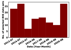
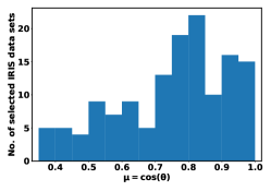
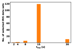
Figure 1: Distribution of the selected data in the $IRIS^{2+}$ database with respect the observation date (left), the position in the solar disk given by $\mu=cos(\theta)$ - with $\theta$ the heliocentric angle (middle), and the exposure time (right).

2.1 Selection of spectral lines

IRIS	Fe I	Ni II	C I	Fe I	Mg II h	Mg II UV3&2	Mg II k	Fe I	Mg II UV1	Ti II
linelist	2827.33	2815.18	2810.58	2809.15	2803.53	2798.85&.72	2796.35	2793.22	2791.60	2785.46
v36_00 & v38_00		✓		✓	✓	✓	✓	✓	✓
v36_01 & v38_01		✓			✓	✓	✓
v36_02 & v38_02		✓				✓	✓
v36_03 & v38_03	✓	✓			✓	✓	✓	✓	✓
v36_04 & v38_04	✓	✓	✓	✓	✓	✓	✓	✓	✓	✓
v40_00					✓	✓	✓			✓
v40_02					✓		✓
v40_09	✓	✓	✓	✓	✓	✓	✓	✓	✓	✓

Table 1: Availability of the spectral lines (in Å) considered in the $IRIS^{2+}$ for each observation IRIS linelist. The C II 1334 & 1335 Å lines, not included in the table, are always included in any IRIS linelist, therefore, they are always considered by $IRIS^{2+}$.

Another important issue is the selection of the photospheric spectral lines. We have tried different combinations of photospheric lines located in the near ultra-violet (NUV) spectral range observed by IRIS. The bottom panel in Figure 2 shows the full spectrum taken by IRIS in its NUV channel. In the top panel of this figure, an average profile of the quiet sun observed at the center of the solar disk is shown. The selected photospheric lines are indicated by vertical lines (orange in the bottom, black in the top panel), while the chromospheric lines, i.e. the Mg II h&k lines and the Mg II UV triplet lines, are similarly indicated in violet. The full spectrum along the slit that is shown in the bottom panel of this figure is intended to help the comparison with the IRIS linelist images that illustrate the combination of spectral ranges selected in an IRIS observation. Because of these linelists (which are used for telemetry reasons, i.e., to minimize the data volume that is downlinked), we have to take into account the availability of the selected lines in the different IRIS observation setups or linelists. Table 1 shows which selected lines are available in the IRIS linelists. Note that in our study, in addition to the lines observed in the NUV channel, we also consider the C II 1334 & 1335 Å lines recorded in the far ultraviolet (FUV) channel.

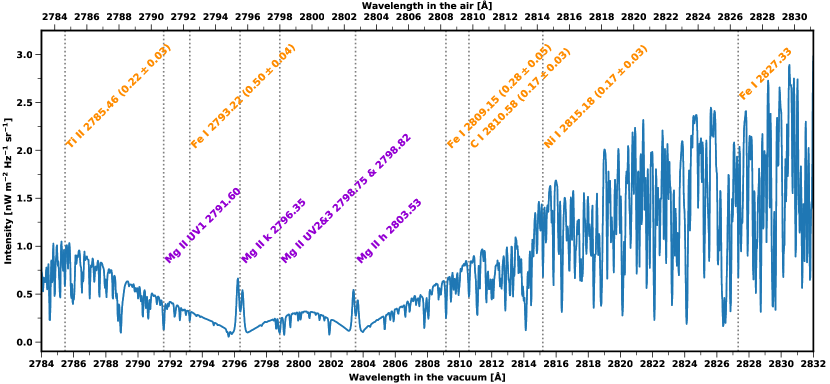
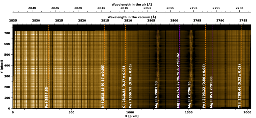
Figure 2: Top: The photospheric (orange) and chromospheric (violet) selected lines in the spectral range observed by IRIS around the Mg II h&k lines. The values in parenthesis indicate the approximate height (in $Mm$) for an optical depth of 1, and the uncertainty associated with the fact that the formation occurs in a corrugated layer, as obtained by Pereira et al. (2013). Bottom: The spectrum as seen on the detector is shown for a better comparison with the IRIS linelist files, e.g. v36_01, which show all the spectral ranges selected for a given observation. Note that wavelength increases towards the left in this panel.

The selection of the photospheric lines is intended to recover as accurately as possible the variation of thermodynamics from the bottom to the top of the photosphere. This information is derived from the response function (RF, Mein, 1971; Landi Degl’Innocenti & Landi Degl’Innocenti, 1981) of the intensity profiles to a variation in a given physical parameter, and from the height at which the optical depth is above 1, as obtained by Pereira et al. (2013). For all the photospheric lines in the panels of Figure 2 - except Fe I 2827.33 Å- the height is provided in $Mm$. including the range of heights that maps velocities in the model to observed line shifts, associated with the fact that the line formation occurs in a corrugated layer. The height estimates are based on the synthesis of these lines using a modified version of the RH code (Uitenbroek, 2001; Pereira & Uitenbroek, 2015) on a 3D radiative MHD numerical simulation obtained by the Bifrost code (Gudiksen et al., 2011) . The RFs of the intensity (for a multi-line RP in the database) to the variation of the temperature is shown in the left panel in Figure 3. Note that the optical depth range where a spectral line is sensitive to the variation of a physical parameter is slightly different for different solar features (e.g., umbra, penumbra, filament, plage), and it is also different for the various physical parameters (temperature, electron density, LOS velocity, microturbulence). The right panel in Figure 3 shows the optical depth ranges where the selected lines in the $IRIS^{2+}$ are roughly sensitive to changes in the temperature. As mentioned above, these ranges summarize the general behavior of the selected lines for most of the observed solar features in the database. They should be understood as a reference of where the lines are mostly sensitive to changes in the thermodynamics.

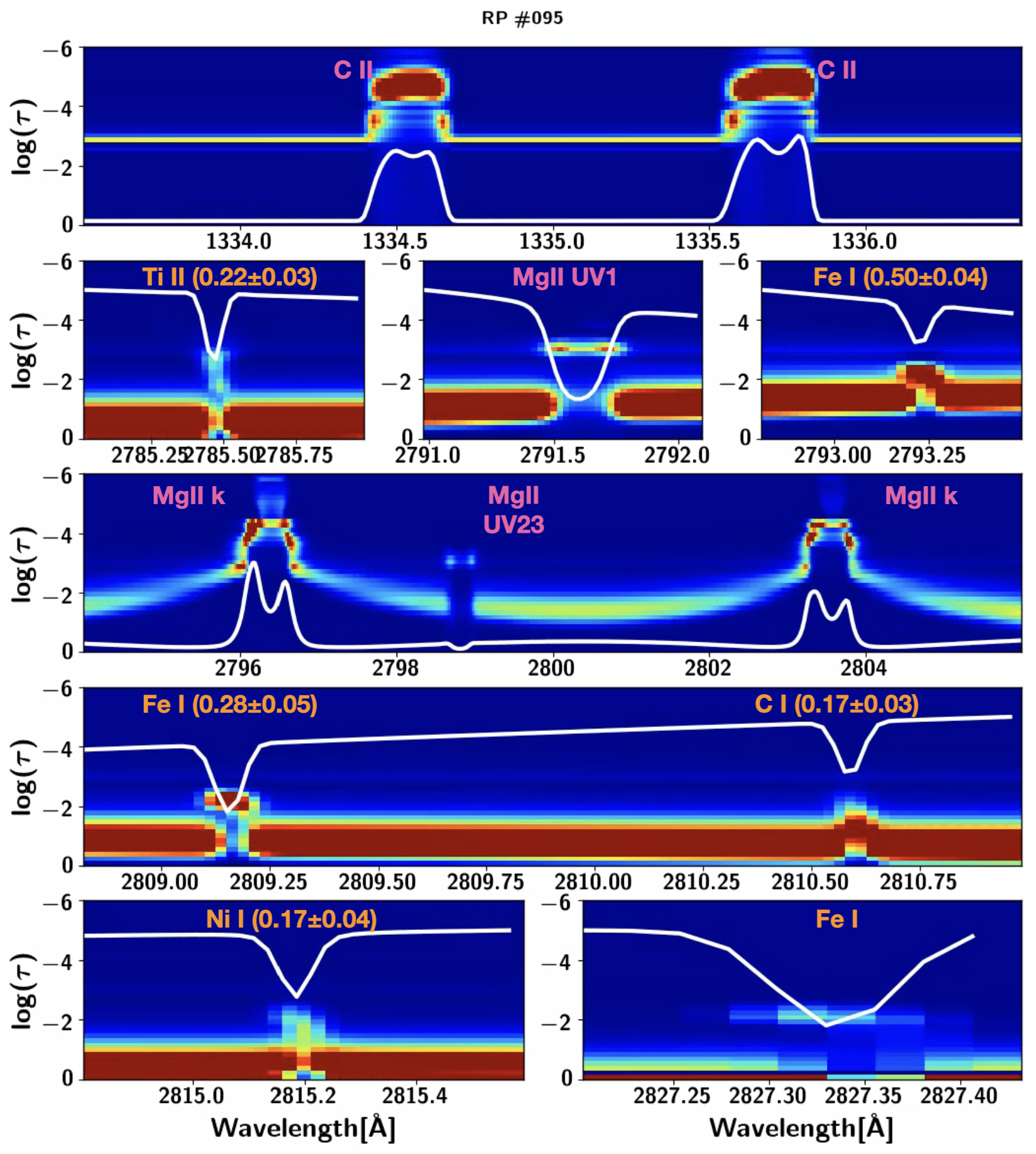
Figure 3: Left: Response function (RF) of the intensity to variations of $T$ of the selected lines in the $IRIS^{2}$ database. The spectral lines (white) are shown as a reference. Right: the optical depth ranges where these lines are on average sensitive to changes of $T$ for the solar features included in the $IRIS^{2+}$ database. Note that these ranges may slightly vary for each solar feature and for the other physical parameters in the database. The values under the lines are given in Å. The values between parenthesis are given in $Mm$. See Figure 2 for details.

2.2 Multi-line representative profiles

Now that we have selected a set of spectral lines that is sensitive to the thermodynamics from the top of the chromosphere to the bottom of the photosphere, the next steps is to prepare them for clustering. The need for clustering our data is due to the computational resources needed to recover the physical information encoded in the spectral lines, specifically when we are working with the C II 1334 & 1335 Å and the Mg II h&k lines. As we have already mentioned the inversion of the latter requires consideration of non-LTE and partial frequency redistribution of the scattered photons. Therefore, we follow the same approach introduced by Sainz Dalda et al. (2019), which was extended by Woods et al. (2021) for the multi-line case of C II 1334 & 1335 Å lines and Mg II h&k (including Mg II UV2&3 lines), and more recently by Sainz Dalda & De Pontieu (2022a) for the multi-line case of C II 1334 & 1335 Å lines, Mg II h&k and all the Mg II UV triplet lines. Now, in addition to the set of chromospheric lines used by the latter authors we include 6 photospheric lines. Because we are now simultaneously considering lines sensitive to the thermodynamics at different optical depths we may have RPs which share the same chomospheric physical conditions but different photosperic thermodynamic conditions, or the other way around. In other words, identical chromospheric profiles may be associated with photospheric profiles that are quite different, or vice versa. We must consider this degeneracy between the chromospheric set of lines and the photospheric set of lines when clustering them. Thus, compared to inversions that are based on fewer lines, we need to consider a larger number of clusters and RPs to capture properly that degeneracy. We have determined that 320 clusters per data set are able to represent properly most of the data sets considered in our study within the hardware limitations we have.

In this investigation, since we are interested in obtaining thermodynamic models for the ARs we have stratified the data before clustering. That means, we have first identified those locations where the profiles belong to the umbra (or pore), the penumbra, the plage, and the quiet Sun. These four regions are determined by using different intensity thresholds in the reconstructed intensity map at $2810.58~{}$Åof the data set to be clustered. The 3 first panels in the top row of Figure 4 show the intensity spectroheliogram or map for an AR at Mg II k, Ti 2 2785.46 Å and at 2832.04 Å (photospheric continuum) respectively. The fourth panel shows the areas identified as umbra, penumbra, plage, and quiet sun. Once these areas are determined, we impose the number of clusters for each region to be clustered. The number of clusters for each region is based on the average area covered by these regions and the variability of different physical conditions in these areas. For instance, the quiet Sun occupies more area in most of the data selected compared to the penumbra. On the other hand, the physical conditions are likely more variable in the latter, although that is not necessary true in the chromosphere. We have attempted to find a trade-off between the hardware limitations (to consider at most 320 RPs per data set) and to recover a meaningful representation of the physics of the selected areas in each data set. The number of clusters for the umbra, penumbra, plage and quiet-sun are 30, 50, 80, 160 respectively. If there is no umbra, i.e., no umbra has been detected under the threshold level established, then the features detected are usually pores, orphan-penumbras, or naked-sunspots. In this case, the number of clusters for the penumbra are incremented up to 80, and the associated RPs are labeled as ’pore-like’. If there is neither umbra nor penumbra, the number of clusters for the plage and quiet Sun are 144 and 176 respectively. In total, the $IRIS^{2+}$ database has $2,280$ RPs associated with the umbra, $800$ RPs with the pore-like features, $3,800$ RPs with the penumbra, $12,640$ with plage, and $20,800$ RPs with quiet Sun. To cluster the original IRIS profiles we created a joint-profile by cropping the selected lines and concatenating them together. These new profiles are scaled between 0 and 1, then they are clustered with the number of clusters determined by the criteria mentioned above. After the clusters are defined, we calculated the RPs (centroids) as the average of the original profiles, i.e. un-cropped, and associated with the elements (labels) of each cluster. At this point, the RPs preserve the original spectral sampling and the original spectral range of the selected lines. They are ready for the inversion.

2.3 Inversion of the Multi-Line Representative Profiles

We have used the multi-atom STockholm inversion Code (STiC de la Cruz Rodríguez et al., 2016, 2019) to invert the RPs of our selected data. STiC is an MPI-parallel non-LTE inversion code that utilises a modified version of RH (Uitenbroek, 2001) to solve the atomic population densities assuming statistical equilibrium and plane-parallel geometry and it allows including partial frequency redistribution effects of scattered photons (Leenaarts et al., 2012). The radiative transport equation is solved using cubic Bezier solvers (de la Cruz Rodríguez & Piskunov, 2013). The inversion engine of STiC includes an equation of state extracted from the SME code (Piskunov & Valenti, 2017).

An important step in the multi-line inversion is needed to properly handle the strong intensity differences between the various lines. This is particularly important for the C II 1334 & 1335 Å lines since their intensity is much than the Mg II h&k, the Mg II UV triplet lines, and the nearby photospheric lines. Therefore, for the inversion we must scale them with respect to the other lines. We have also considered this between the Mg II UV2&3 lines with respect to the Mg II h&k lines, and the photospheric lines with respect to the Mg II h&k lines. The strategy is as follows: we calculate the most frequent value of the intensity in a spectroheliogram map in the Mg II h&k $k_{3}$, and we scale or weight the C II 1334 & 1335 Å lines to that value. That means, we try to scale the C II 1334 & 1335 Å lines to the same relative intensity level as the Mg II h&k lines. Note that a somewhat similar strategy was used by Sainz Dalda & De Pontieu (2022a). However, in that case, because the authors were investigating the thermodynamics of the chromosphere during the maximum of a X1.0-class flare, the ratio between the maximum intensity in the Mg II h&k lines and the C II 1334 & 1335 Å lines varies from $\approx 100$ in the non-flaring region to just $\approx 10$ in the ribbons, both in the same FoV or dataset. Therefore, the authors decided to stratify the data considering different populations of profiles with different intensity. As a consequence, different weights for the C II 1334 & 1335 Å lines with respect to the Mg II h&k lines were used for different regions in a data set.The need for this scaling (or weighting) is due the different behavior of the lines in different solar features, with the most extreme differences occurring between the non-flaring and flaring regions. The data sets considered in this study do not have such a strong variation of intensity between the C II 1334 & 1335 Å and Mg II h&k lines in different regions within the same field of view. Therefore, only one weight is used for the C II 1334 & 1335 Å lines for the full data set. For the Mg II UV1 line, the Mg II UV2&3 lines, and the photospheric lines we used a slightly different strategy. For these lines we obtained the weights with respect to the Mg II h&k lines in an empirical fashion, after we verified that using the strategy of the most frequent value of the Mg II h&k $k_{3}$ map did not provide a significant advantage. In other words, we found that for these lines, on average, the relative intensity with respect to that of the Mg II h&k lines for different data sets has a small standard deviation. Thus, for the sake of simplicity, we have used the same combination of weights (with respect to Mg II h&k) for these lines. For a dataset, STiC only accepts a wavelength-dependent noise and weight for all the profiles. For simplicity, the noise is the same averaged noise (standard deviation in a spectral range) at all the wavelengths, while the different weights are given for different spectral positions (usuallly ranges or windows). That means, we use an unique value of the $w_{i}/\sigma$ per data set in the merit function used to quantify the quality of the fit between the observed $I(\lambda_{i})^{obs}$, and the inverted profile $I(\lambda_{i},\mathbf{M})^{syn}$, that is:

$$\chi^{2}=\frac{1}{\nu}\sum_{i=0}^{q}{(I(\lambda_{i})^{obs}-I(\lambda_{i},\mathbf{M})^{syn})^{2}\frac{w_{i}^{2}}{\sigma_{i}^{2}}}$$ (1)

with $i=0,...,q$ the sampled wavelengths, $w_{i}$ their weights, $\sigma_{i}$ the uncertainties of the observation (e.g. photon noise), and $\nu$ the number of spectral samples. Note that we assume, for simplicity, that $\sigma_{i}$ is the same for all $i$, as mentioned above. We have used 3 cycles with different number of nodes for the physical variables in the model. These values are detailed in the table 2. We used the FALC quiet-sun model (Fontenla et al., 1993) as the initial guess model for all the inversions.

No. Cycle	1	2	3
$T$	4	7	9
$v_{turb}$	2	4	8
$v_{los}$	2	4	8

Table 2: Number of nodes in each cycle for the thermodynamics variables considered during the inversions.

3 Results

Figures 4 and 5 show the inversion of a multi-line RP in the penumbra and the outer part of the plage of the NOAA 12681, respectively, both on 2017-09-26 at 05:09:50UT. In addition to the observed RP (in fuchsia) and its corresponding inverted, synthetic RP (best fit obtained by STiC, in black), the temperature ($T$), line-of-sight velocity ($v_{los}$), the velocity of turbulent motions or micro-turbulence ($v_{turb}$), and the logarithm of the electron density ($n_{e}$) are shown in the last row of these figures. The rest position of the lines is indicated with a vertical dashed line. The inset plots in the fourth row show the core of the Mg II h&k and Mg II UV2&3 lines.

As a result of the strategy presented in this article, we have an indexed, labeled, relational data base. Thus, each inverted synthetic RP has an associated representative model atmosphere (RMA), and the following meta-data: the IRIS filename and the solar feature (“umbra”, “penumbra”, “pore-like”, “plage”, and “quiet-sun”) where the RP was clustered, the position on the Sun of the original observed profiles associated with the RP’s cluster, the exposure time, and the observation time. Because information is attached to the RP-RMA pair in $IRIS^{2+}$  one can search for RMAs for a given solar feature (e.g. ’plage’), at a given time in the solar cycle (e.g. ’2014-01-01’ $<$ date_obs $<$ ’2014-05-31’), and at given position on the Sun. Figure 6 shows the case of a search of the RMAs for all the solar features located at $0.65<\mu<0.70$. As one would expect, the RMAs show, for a given physical parameter, some variation both within the same solar feature (e.g., the $v_{turb}$ for the RMAs in the plage), and between solar features (e.g umbra versus penumbra). In this example search, only 2 umbras (30 RMA/umbra) and 2 penumbras (50 RMA/penumbra) were observed and included in the data base. In fact, these 2 umbras and 2 penumbras observations belong to the same AR, and for that reason the dispersion between the RMAs for the different physical variables is rather small in these solar features. Several plages and "quiet-sun" belonging to different ARs are however found in this search, and for that reason their associated RMAs show a larger variability. We remind the reader that the term "quiet-sun" here refers to regions within an active region that are not plage, umbra, pores, or penumbra. It is not evident that such regions are, in fact, identical to quiet Sun regions that are not part of an active region. This is because the overlying large-scale magnetic field topology and the associated canopy can impact the chromosphere of these regions, which are at the photospheric level perhaps more quiet-Sun like.

The quality of the inversion is not always easy to evaluate from the $\chi^{2}$ value in the profiles of $IRIS^{2+}$. This is because of the behavior of the Euclidean distance when applied to problems with high dimensions, which is the case of our profiles. In many cases, a bad fit in the core of the Mg II h&k lines penalizes too much the value of $\chi^{2}$ (see section 3 of Sainz Dalda & De Pontieu 2022b for a more detailed discussion). In addition, we are now using multiple lines. That increases the possibility of having a bad $\chi^{2}$ value when one or a few lines are badly fitted, but the rest are well fitted. Of course, when all the lines are well fitted, the $\chi^{2}$ is good (i.e., low). The question is what to do when several lines are well fitted and others are not (i.e., with a resulting high value for $\chi^{2}$). As we will discuss later, that is not a big problem, since we have verified that in a large majority the profiles are well fitted. Even for the minority of RPs where some lines are badly fitted, there are usually several other lines that are well fitted.

Figure 4: First row: Spectroheliogram map for Mg II h&k $k_{3}$, the Ti I 2785.46 Å, the photospheric continuum at 2832.04 Å, and a map of the various types of regions that were identified (see text). The other rows are results from an inversion for the location marked with a white cross in the “Selected areas” map in the right of the top row. From the second to the sixth row, from left to right, the observed (dotted-solid in fuchsia) and the inverted profile (black) for the C II 1334 & 1335 Å lines, Ti I 2785.46 Å, Mg II UV1  Fe I 2793.22 Å, Mg II h&k lines - including Mg II UV2&3-, Fe I 2809.15 Å, C I 2810.58 Å, Ni I 2815.18 Å, and Fe I 2827.33 Å. The bottom row shows the temperature ($T$, orange), the logarithm of the electron density ($n_{e}$, violet), velocity of turbulent motions or micro-turbulent ($v_{turb}$, green) and the line-of-sight ($v_{los}$, blue). Both the inverted profile and the representative model atmosphere (RMA) are included in the $IRIS^{2+}$, and they are both labeled as penumbra in the database.

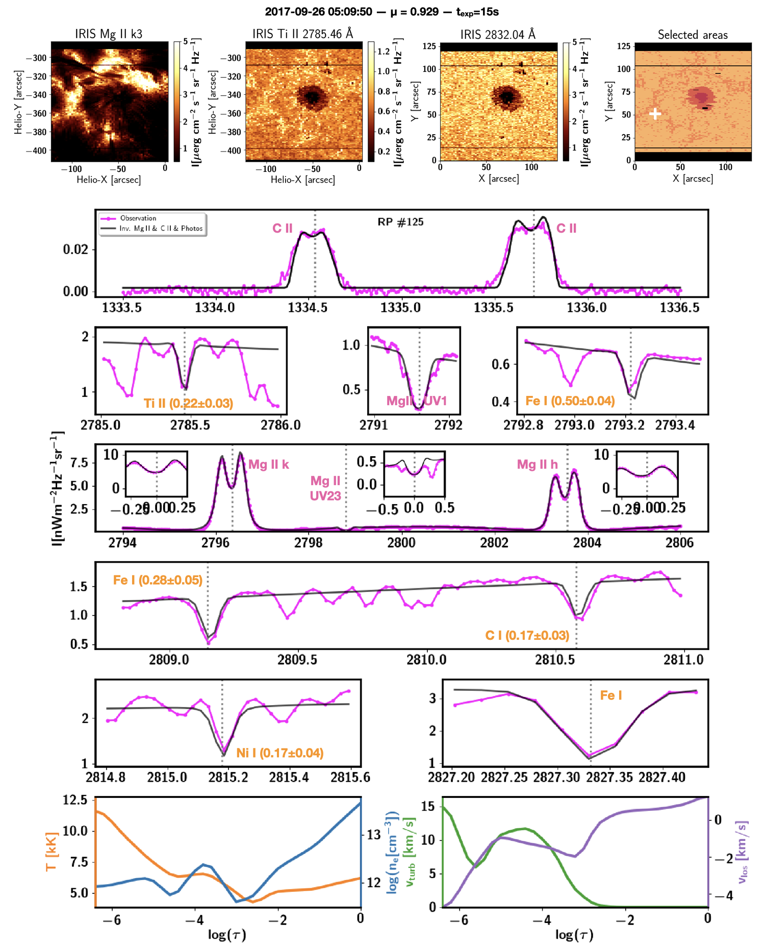
Figure 5: Same as Figure 4 for a multi-line RP and RMA in the outer plage (marked with a white cross in the “Selected areas" panel). Both the inverted profile and eh representative model atmosphere (RMA) are included in the $IRIS^{2+}$, and they are both labeled as ’plage’ in the database.

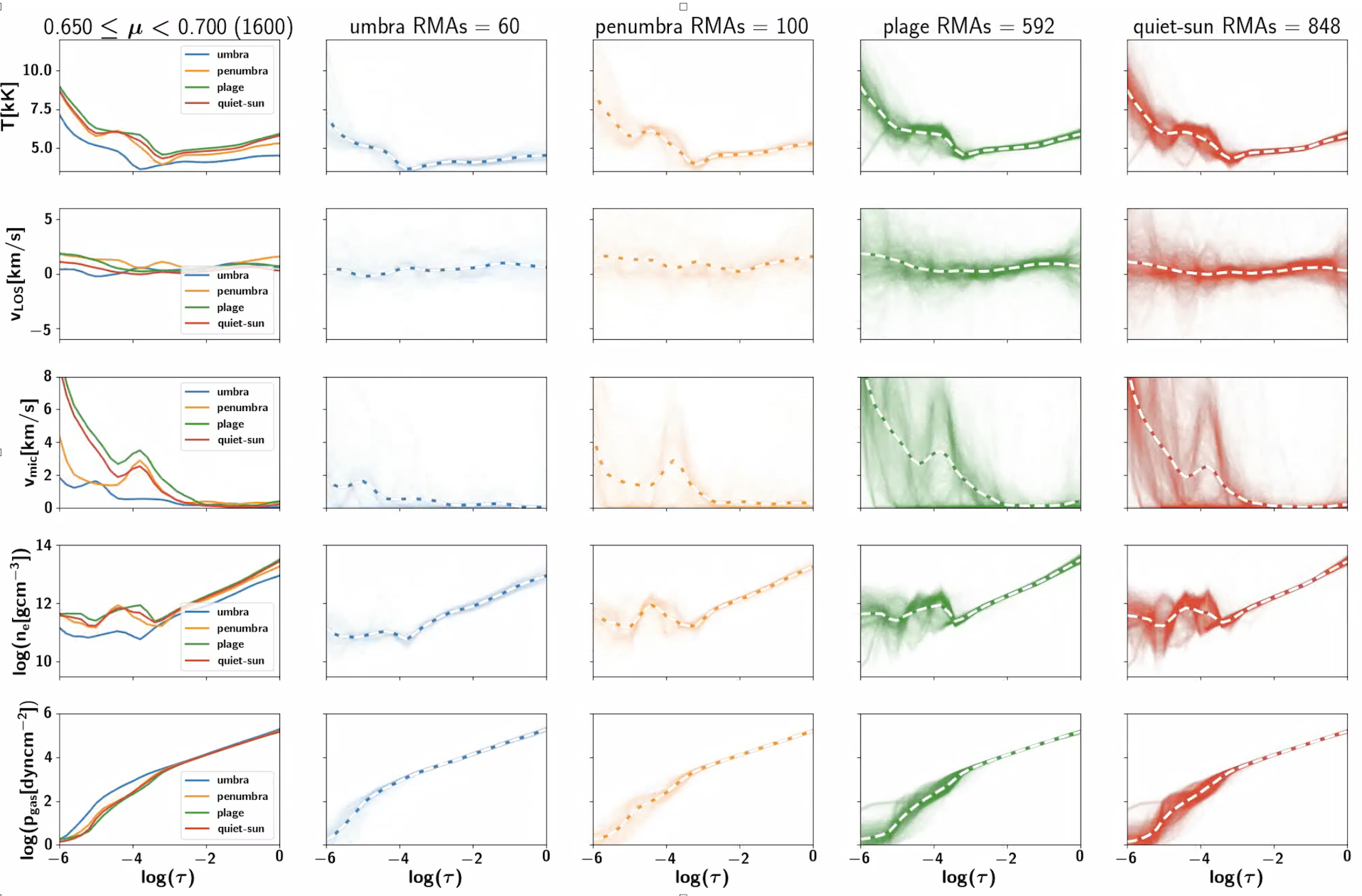
Figure 6: Using $IRIS^{2+}$ data base to find and visualize the different models of umbra, penumbra, plage and quiet-sun at a given interval of $\mu=cos(\theta)$, with $\theta$ the heliocentric angle.

4 Discussion

In the example of the $IRIS^{2+}$ data base shown in Figure 4, the inverted profiles fit the observed profiles very well. Therefore, we can be confident with the representative model atmosphere (RMA) obtained, and because the fit is very good for all the lines, the uncertainty of the physical values should be rather small at all the optical depth ranges shown in the right panel of Figure 3, i.e., where the RFs are large. What if one or more lines are not fitting well the observed profile? A very picky reader might consider that is the case, for instance, for the lines Fe I 2793.22 Å, Fe I 2809.15 Å, C I 2810.58 Å, and Ni I 2815.18 Å. In this case, the reader should consider the values at the optical depths $-3<$ $log(\tau)$$<-1$ with some caution, since only Fe I 2827.33 Åis fitting the observed profile very well. Which impact do the lines that do not fit the observations well have in the $IRIS^{2+}$? Strictly speaking, none. The $IRIS^{2+}$ database is a relational data base between model atmospheres and their synthetic profiles. The physics encoded in the latter are strictly due to the values in the model atmosphere and the considerations made to solve the radiative transfer equation. Practically speaking, it has an impact if the fits were consistently bad - which is not the case.

The $IRIS^{2}$ can be used in different ways: as a set of reference model atmospheres and profiles for the various types of features within ARs; as constraints for numerical models; as a look-up table for speeding inversions problems; or as a source atmosphere to synthesize spectral lines both in the chromosphere and the photosphere, including full-Stokes polarimetric profiles by considering magnetic field information. In all these cases, we want to have a better representation of the thermodynamics in the low solar atmosphere, and in that sense the better the fits are, the better that representation is. However, those synthetics profiles that show some poorer fits with respect to the observed RP very likely still occur in the solar atmosphere. Therefore, since a very large number of the inversions calculated to build the $IRIS^{2+}$ data base are showing very good fits, we consider this database likely the most accurate comprehensive set of stratified-depth models and profiles in the chromosphere and the photosphere.

5 Conclusions

Thanks to the extraordinary multi-line capabilities of IRIS, we have created a database of 40,320 synthetic representative profiles and their corresponding representative model atmospheres that convey the essential thermodynamic information of active regions from the bottom of the photosphere to the top of the chromosphere.

Thanks to the state-of-the-art multi-line multi-atom STiC inversion code, we have been able to recover the physical information encoded in 6 chromospheric lines and 6 photospheric lines. Using the well-known k-means technique we have clustered multi-line IRIS spectral data. This helps us to overcome the task of inverting all the profiles considered in this work, which would require very significant computational resources ($\approx 242,000~{}CPU-hours$).

$IRIS^{2+}$ is an unique data base, obtained systematically from an unprecedented combination of a large number spectral lines sensitive to the thermodynamics in the low solar atmosphere. We will continue maximizing the observational capabilities of IRIS, considering more lines and applying improved inversion methods and advance machine learning techniques. $IRIS^{2+}$ has a high potential to be used in different ways to gain knowledge in the low solar atmosphere. $IRIS^{2+}$, as well as $IRIS^{2}$ already is, will be available to the public in different formats, both for IDL and Python. We encourage the community to exploit $IRIS^{2+}$ to solve the physics of the ARs.

References

- Bjørgen et al. (2019) Bjørgen, J. P., Leenaarts, J., Rempel, M., et al. 2019, A&A, 631, A33
- Carlsson et al. (2019) Carlsson, M., De Pontieu, B., & Hansteen, V. H. 2019, ARA&A, 57, 189
- Cauzzi et al. (2008) Cauzzi, G., Reardon, K. P., Uitenbroek, H., et al. 2008, A&A, 480, 515
- Collados et al. (1994) Collados, M., Martinez Pillet, V., Ruiz Cobo, B., del Toro Iniesta, J. C., & Vazquez, M. 1994, A&A, 291, 622
- de la Cruz Rodríguez et al. (2016) de la Cruz Rodríguez, J., Leenaarts, J., & Asensio Ramos, A. 2016, ApJ, 830, L30
- de la Cruz Rodríguez et al. (2019) de la Cruz Rodríguez, J., Leenaarts, J., Danilovic, S., & Uitenbroek, H. 2019, A&A, 623, A74
- de la Cruz Rodríguez & Piskunov (2013) de la Cruz Rodríguez, J., & Piskunov, N. 2013, ApJ, 764, 33
- del Toro Iniesta & Ruiz Cobo (2016) del Toro Iniesta, J. C., & Ruiz Cobo, B. 2016, Living Reviews in Solar Physics, 13, 4
- del Toro Iniesta et al. (1994) del Toro Iniesta, J. C., Tarbell, T. D., & Ruiz Cobo, B. 1994, ApJ, 436, 400
- Fontenla et al. (1993) Fontenla, J. M., Avrett, E. H., & Loeser, R. 1993, ApJ, 406, 319
- Fontenla et al. (2009) Fontenla, J. M., Curdt, W., Haberreiter, M., Harder, J., & Tian, H. 2009, ApJ, 707, 482
- Gingerich et al. (1971) Gingerich, O., Noyes, R. W., Kalkofen, W., & Cuny, Y. 1971, Sol. Phys., 18, 347
- Gudiksen et al. (2011) Gudiksen, B. V., Carlsson, M., Hansteen, V. H., et al. 2011, A&A, 531, A154
- Hale (1908) Hale, G. E. 1908, PASP, 20, 220
- Khomenko et al. (2014) Khomenko, E., Collados, M., Díaz, A., & Vitas, N. 2014, Physics of Plasmas, 21, 092901
- Landi Degl’Innocenti & Landi Degl’Innocenti (1981) Landi Degl’Innocenti, E., & Landi Degl’Innocenti, M. 1981, Nuovo Cimento B Serie, 62B, 1
- Leenaarts et al. (2012) Leenaarts, J., Pereira, T., & Uitenbroek, H. 2012, A&A, 543, A109
- Leenaarts et al. (2013) Leenaarts, J., Pereira, T. M. D., Carlsson, M., Uitenbroek, H., & De Pontieu, B. 2013, ApJ, 772, 89
- Martínez-Sykora et al. (2020) Martínez-Sykora, J., Leenaarts, J., De Pontieu, B., et al. 2020, ApJ, 889, 95
- Mein (1971) Mein, P. 1971, Sol. Phys., 20, 3
- Pereira et al. (2013) Pereira, T. M. D., Leenaarts, J., De Pontieu, B., Carlsson, M., & Uitenbroek, H. 2013, ApJ, 778, 143
- Pereira & Uitenbroek (2015) Pereira, T. M. D., & Uitenbroek, H. 2015, A&A, 574, A3
- Piskunov & Valenti (2017) Piskunov, N., & Valenti, J. A. 2017, A&A, 597, A16
- Rutten (2007) Rutten, R. J. 2007, in Astronomical Society of the Pacific Conference Series, Vol. 368, The Physics of Chromospheric Plasmas, ed. P. Heinzel, I. Dorotovič, & R. J. Rutten, 27
- Sainz Dalda et al. (2019) Sainz Dalda, A., de la Cruz Rodríguez, J., De Pontieu, B., & Gošić, M. 2019, ApJ, 875, L18
- Sainz Dalda & De Pontieu (2022a) Sainz Dalda, A., & De Pontieu, B. 2022a, submitted
- Sainz Dalda & De Pontieu (2022b) —. 2022b, submitted
- Sukhorukov & Leenaarts (2017) Sukhorukov, A. V., & Leenaarts, J. 2017, A&A, 597, A46
- Uitenbroek (2001) Uitenbroek, H. 2001, ApJ, 557, 389
- Wargnier et al. (2022) Wargnier, Q. M., Martinez-Sykora, J., Hansteen, V. H., & De Pontieu, B. 2022, arXiv e-prints, arXiv:2211.02157
- Wedemeyer et al. (2016) Wedemeyer, S., Bastian, T., Brajša, R., et al. 2016, Space Sci. Rev., 200, 1
- Woods et al. (2021) Woods, M. M., Sainz Dalda, A., & De Pontieu, B. 2021, ApJ, 922, 137