Comparative Learning: A Sample Complexity Theory for Two Hypothesis Classes

Abstract

In many learning theory problems, a central role is played by a hypothesis class: we might assume that the data is labeled according to a hypothesis in the class (usually referred to as the realizable setting), or we might evaluate the learned model by comparing it with the best hypothesis in the class (the agnostic setting). Taking a step beyond these classic setups that involve only a single hypothesis class, we study a variety of problems that involve two hypothesis classes simultaneously.

We introduce comparative learning as a combination of the realizable and agnostic settings in PAC learning: given two binary hypothesis classes $S$ and $B$, we assume that the data is labeled according to a hypothesis in the source class $S$ and require the learned model to achieve an accuracy comparable to the best hypothesis in the benchmark class $B$. Even when both $S$ and $B$ have infinite VC dimensions, comparative learning can still have a small sample complexity. We show that the sample complexity of comparative learning is characterized by the mutual VC dimension ${\mathsf{VC}}(S,B)$ which we define to be the maximum size of a subset shattered by both $S$ and $B$. We also show a similar result in the online setting, where we give a regret characterization in terms of the analogous mutual Littlestone dimension ${\mathsf{Ldim}}(S,B)$. These results also hold for partial hypotheses.

We additionally show that the insights necessary to characterize the sample complexity of comparative learning can be applied to other tasks involving two hypothesis classes. In particular, we characterize the sample complexity of realizable multiaccuracy and multicalibration using the mutual fat-shattering dimension, an analogue of the mutual VC dimension for real-valued hypotheses. This not only solves an open problem proposed by Hu, Peale, Reingold (2022), but also leads to independently interesting results extending classic ones about regression, boosting, and covering number to our two-hypothesis-class setting.

1 Introduction

The seminal theoretical framework of PAC learning [Valiant, 1984] provides a formalization of machine learning that allows for rigorous theoretical analysis. In PAC learning, a learning algorithm (learner) receives individual/label pairs $(x,y)\in X\times\{-1,1\}$ as input data, drawn i.i.d. from an unknown distribution $\mu$. The learner’s goal is to output a model $f:X\rightarrow\{-1,1\}$ that assigns each individual in $X$ a binary label. The performance of the model $f$ is measured by its classification error,

$${\mathsf{error}}(f):={\Pr}_{(x,y)\sim\mu}[f(x)\neq y].$$

Because the classification error is evaluated over the entire distribution $\mu$, a good learner must go beyond simply memorizing the individuals and labels seen in the input data and be able to correctly predict the labels of unseen individuals as well. This can be a difficult task, and to make it possible to achieve a meaningfully small error given a limited amount of input data, additional assumptions or relaxations are needed. This leads to two standard settings of PAC learning: realizable and agnostic learning. In realizable learning, we assume that all data points are labeled according to an unknown hypothesis $h:X\rightarrow\{-1,1\}$, i.e., $y=h(x)$ for every data point $(x,y)$ drawn from $\mu$, and we assume that $h$ belongs to a hypothesis class $H$ known to the learner. Under this assumption, realizable learning requires the output model $f$ to achieve a low classification error (${\mathsf{error}}(f)\leq\varepsilon$) with large probability. In agnostic learning there is also a hypothesis class $H$ known to the learner, but it does not impose any assumption on the data. Instead, we aim for a relaxed goal specified by $H$: achieving ${\mathsf{error}}(f)\leq\inf_{h\in H}{\mathsf{error}}(h)+\varepsilon$ with large probability.

At a high level, both realizable and agnostic learning involve the introduction of a hypothesis class $H$, but $H$ plays a very different role in each setting. In realizable learning, $H$ constrains the potential source hypotheses that might determine the ground-truth labeling of the data. In contrast, agnostic learning places no assumptions on the ground-truth labeling, but instead uses $H$ as a benchmark class and only requires the learner to perform well compared to the best benchmark hypothesis in $H$. Thus, realizable and agnostic learning highlight two natural ways to simplify a learning task: constrain the potential hypotheses that the ground-truth labeling is generated from, or constrain the set of hypotheses that the output model is compared against.

Our work originates from the observation that these two ways of simplifying a learning task need not be mutually exclusive. Instead, they can be treated as two “knobs” that can be simultaneously adjusted to create new hybrid learning tasks. For any two hypothesis classes $S$ and $B$, we can define a learning task by letting them play the two roles of $H$ in the realizable and agnostic settings, respectively. That is, we assume that there exists a source hypothesis $s\in S$ such that $y=s(x)$ for every data point $(x,y)$ drawn from $\mu$, and we aim for achieving, with large probability, an error comparable to the best benchmark hypothesis $b\in B$: ${\mathsf{error}}(f)\leq\min_{b\in B}{\mathsf{error}}(b)+\varepsilon$. We term this hybrid notion comparative learning.

Our research reveals that the notion of comparative learning is far more insightful than just a thought experiment: it serves as an unexplored playground for the study of sample complexity, and the new connections we establish to characterize the sample complexity of comparative learning can be fruitfully applied to open questions about existing learning tasks. Here, “sample complexity” refers to one of the key characteristics of every learning task: the minimum number of data points needed by a learner to solve the task. VC theory provides a thorough understanding of the sample complexity of classic PAC learning in both the realizable and agnostic settings: in both cases it is characterized by the VC dimension of the hypothesis class $H$, defined as the maximum size of a subset of $X$ on which all possible labelings of the individuals can be realized by some hypothesis in $H$ (we say a set is shattered by $H$ when this condition holds; see Section 2 for the exact definition) [Vapnik and Chervonenkis, 1971, Blumer et al., 1989, Linial et al., 1991]. Since then, understanding the sample complexity of a wide variety of new and existing learning tasks has remained an exciting area of research. These tasks include online learning [Littlestone, 1988, Ben-David et al., 2009, Alon et al., 2021, Filmus et al., 2022], reliable and useful learning [Rivest and Sloan, 1989, Kivinen, 1989, 1995, 1990], statistical query learning [Kearns, 1993, Blum et al., 1994], learning real-valued hypotheses [Kearns and Schapire, 1994, Alon et al., 1993, Bartlett et al., 1996], multiclass learning [Ben-David et al., 1995, Brukhim et al., 2022], learning partial hypotheses [Long, 2001, Alon et al., 2022], active learning [Balcan et al., 2009, 2010, Kane et al., 2017, Hopkins et al., 2020c, b, a], property testing [Goldreich et al., 1996, Kearns and Ron, 2000, Blais et al., 2021], differentially private learning [Alon et al., 2019, Bun et al., 2020, Ghazi et al., 2021, Sivakumar et al., 2021, Jung et al., 2020, Golowich, 2021], bounded-memory learning [Gonen et al., 2020], and online learning in the smoothed analysis model [Haghtalab et al., 2020, 2022]. A commonality of these learning tasks is that each of them only explicitly involves a single hypothesis class, and thus the sample complexity is studied in terms of complexity measures of single hypothesis classes, such as the VC dimension, the Littlestone dimension, the statistical query dimension, the fat-shattering dimension, and the DS dimension. To tightly characterize the sample complexity of comparative learning where a pair of hypothesis classes $S$ and $B$ are involved, it is not sufficient to apply existing complexity measures to $S$ and $B$ separately (see Section 1.1 for a more detailed discussion). Instead, we must create new notions that measure the complexity of the interaction between the two classes. We show that the correct way to measure the complexity of this interaction in comparative learning is to look at the subsets of $X$ that $S$ and $B$ both shatter, and we define the mutual VC dimension, ${\mathsf{VC}}(S,B)$, to be the maximum size of such subsets. We show that the mutual VC dimension gives both upper and lower bounds on the sample complexity of comparative learning. Similarly, in an online analogue of comparative learning, we define the mutual Littlestone dimension and prove upper and lower regret bounds.

Our sample complexity characterization for comparative learning turns out to be a powerful tool for studying the sample complexity of other tasks involving two hypothesis classes. In fact, our interest in comparative learning is derived in part from open questions related to the sample complexity of realizable multiaccuracy (MA) and multicalibration (MC) [Hébert-Johnson et al., 2018, Kim et al., 2019, Hu et al., 2022b]. In these tasks, the hypothesis class $H$ plays the same role as in realizable learning, while the classification error ${\mathsf{error}}(f)$ is replaced with an alternative error measure ${\textnormal{MA-error}}_{D}(f)$ or ${\textnormal{MC-error}}_{D}(f)$ specified by an additional hypothesis class $D$ that is sometimes called the distinguisher class. For example, the multiaccuracy error ${\textnormal{MA-error}}_{D}(f)$ is defined as follows:

$${\textnormal{MA-error}}_{D}(f):={\sup}_{d\in D}|{\mathbb{E}}_{(x,y)\sim\mu}[(f(x)-y)d(x)]|,$$

where the supremum is over all the distingushers $d:X\rightarrow[-1,1]$ in the distinguisher class $D$. As demonstrated by Hu, Peale, and Reingold [2022b], the freedom in choosing the class $D$ allows the error to adapt to different goals that may arise in practice.

The introduction of the distinguisher class $D$ makes sample complexity characterization challenging because the characterization needs to depend on both the class $H$ in realizable learning and the additional distinguisher class $D$. Hu, Peale, and Reingold [2022b] give a sample complexity characterization for realizable multiaccuracy using a particular metric entropy defined for every pair $(H,D)$ (see Section 1.2 for more details), but their characterization is in the distribution-specific setting where the marginal distribution $\mu|_{X}$ of $x$ in a pair $(x,y)$ generated from the data distribution $\mu$ is fixed and known to the learner. In contrast, the VC dimension characterization for PAC learning is in the distribution-free setting where the learner has no explicit knowledge about $\mu|_{X}$ and must perform well for every $\mu|_{X}$. The sample complexity characterization for realizable multiaccuracy in the distribution-free setting is left as an open question by Hu, Peale, and Reingold [2022b].

In this work, we answer this open question by characterizing the sample complexity of realizable multiaccuracy and multicalibration in the distribution-free setting using the mutual fat-shattering dimension, which we define similarly to the mutual VC dimension but for two real-valued hypothesis classes. Our results on comparative learning turn out to be especially useful for obtaining this characterization because there is an intimate relationship between achieving the comparative learning goal ${\mathsf{error}}(f)\leq\min_{b\in B}{\mathsf{error}}(b)+\varepsilon$ and achieving a low multiaccuracy (or multicalibration) error: ${\textnormal{MA-error}}_{B}(f)\leq\varepsilon$. Here, the benchmark class $B$ in comparative learning plays the role of the distinguisher class $D$ in multiaccuracy and multicalibration. This relationship has been observed by Hébert-Johnson, Kim, Reingold, and Rothblum [2018] and Gopalan, Kalai, Reingold, Sharan, and Wieder [2022b] in a single-hypothesis-class setting, i.e., without the assumption that the labels from the data distribution are generated according to a hypothesis in a pre-specified source class. We generalize this relationship to our two-hypothesis-class setting by showing a reduction from realizable multiaccuracy and multicalibration to comparative learning while preserving the interaction between the source and distinguisher/benchmark classes. This reduction leads to a number of new learning tasks that also involve a pair of hypothesis classes. Specifically, the reduction is accomplished via an intermediate task which we call correlation maximization, and we show that with some adaptation the reduction also allows us to efficiently boost a weak comparative learner to a strong one. Once we achieve multiaccuracy and multicalibration, we apply the omnipredictor result by Gopalan, Kalai, Reingold, Sharan, and Wieder [2022b] to solve comparative regression, an analogue of comparative learning but with real-valued hypotheses and general convex and Lipschitz loss functions. We believe that there is a rich collection of learning tasks where two or more hypothesis classes may interact in interesting ways, and our work is just a small step towards a better understanding of a tiny fraction of these tasks.

1.1 Sample Complexity of Comparative Learning

As mentioned earlier, VC theory has provided a thorough understanding of the sample complexities of both realizable and agnostic learning.

For any binary hypothesis class $H$, VC theory characterizes the sample complexity of realizable and agnostic learning using the VC dimension ${\mathsf{VC}}(H)$ of the hypothesis class $H$, a combinatorial quantity with a simple definition: the maximum size of a subset of $X$ shattered by $H$ (see Section 2 for exact definition) [Vapnik and Chervonenkis, 1971, Blumer et al., 1989, Linial et al., 1991]. Moreover, the optimal sample complexity in both the realizable and agnostic settings can be achieved by a simple algorithm: the empirical risk minimization algorithm (ERM), which outputs the hypothesis in $H$ with the minimum empirical error on the input data points.

Because our notion of comparative learning combines these two settings, it would seem natural to use techniques from VC theory to understand its sample complexity as well. Compared to realizable learning for $S$, comparative learning for $(S,B)$ has a relaxed goal (specified by the benchmark class $B$), and thus any learner solving realizable learning for $S$ also solves comparative learning for $(S,B)$. This gives us a sample complexity upper bound in terms of ${\mathsf{VC}}(S)$ for comparative learning. Similarly, any learner solving agnostic learning for $B$ also solves comparative learning for $(S,B)$ because comparative learning only makes additional assumptions on data (specified by the source class $S$), so we get another sample complexity upper bound in terms of ${\mathsf{VC}}(B)$.

However, perhaps surprisingly, these sample complexity upper bounds provided by the classic VC theory are not optimal. Even when ${\mathsf{VC}}(S)$ and ${\mathsf{VC}}(B)$ are both infinite, comparative learning may still have a finite sample complexity. Imagine that the domain $X$ of individuals is partitioned into two large subsets $X_{1}$ and $X_{2}$. Suppose the source class $S$ consists of all binary hypotheses $s:X\rightarrow\{-1,1\}$ satisfying $s(x)=1$ for every $x\in X_{1}$, and the benchmark class $B$ consists of all binary hypotheses $b:X\rightarrow\{-1,1\}$ satisfying $b(x)=1$ for every $x\in X_{2}$. Both ${\mathsf{VC}}(S)$ and ${\mathsf{VC}}(B)$ can be large and even infinite, but comparative learning in this case requires no data points: the learner can simply output the model $f$ that maps every $x\in X$ to $1$ because no benchmark hypothesis in $B$ can achieve a smaller error than $f$ when the data points $(x,y)\sim\mu$ satisfy $y=s(x)$ for a source hypothesis $s\in S$ (see Figure 1). Beyond demonstrating that comparative learning may require far fewer samples than what our initial naïve upper bound might suggest, this example also shows that the standard empirical risk minimization (ERM) algorithm used for PAC learning does not give us the optimal sample complexity for comparative learning. Assume that the source hypothesis $s\in S$ maps every $x\in X$ to $1$ and $\mu$ is the uniform distribution over $X\times\{1\}$. In this case $\min_{b\in B}{\mathsf{error}}(b)=0$ and thus comparative learning requires a low classification error ${\mathsf{error}}(f)\leq\varepsilon$ with large probability. We have shown that this requirement can be achieved without any input data points, but the ERM algorithm cannot achieve this requirement in general unless there are many input data points: there can be many hypotheses in $S$ and $B$ that achieve zero empirical error on the input data points, but when the data points are few, most of such hypotheses do not achieve low classification error over the entire distribution $\mu$ (see Figure 2).

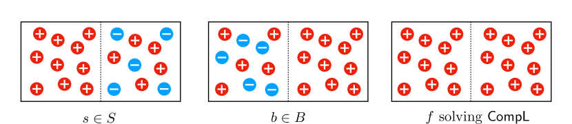
Figure 1: An example where comparative learning requires no data points when ${\mathsf{VC}}(S)$ and ${\mathsf{VC}}(B)$ are both infinite. The left two images show examples of hypotheses in $S$ and $B$, both of which are very complex, but on disjoint portions of the domain. In this case, a learner that always outputs the model $f$ in the rightmost image solves comparative learning because $f$ always achieves smaller or equal error compared to any benchmark hypothesis $b\in B$ when the ground-truth labelling is generated by a source hypothesis $s\in S$. See in-text description for more details.

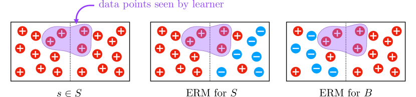
Figure 2: Empirical risk minimization (ERM) may fail to give us optimal sample complexity in the same setting as Figure 1, where $S$ and $B$ are both very complex, but on disjoint domains. When the source hypothesis $s\in S$ is the constant function shown in the left image, the right two images show examples of output models of ERM when run on $S$ and $B$. Neither model is guaranteed to achieve the low error required by comparative learning. See in-text description for more details.

The example above shows that the VC dimensions ${\mathsf{VC}}(S)$ and ${\mathsf{VC}}(B)$ alone are not informative enough to characterize the sample complexity of comparative learning. These VC dimensions only tell us the complexity of $S$ and $B$ separately, but we also need to know the complexity of their interaction. We measure the complexity of this interaction by defining the mutual VC dimension ${\mathsf{VC}}(S,B)$ to be the maximum size of a subset of $X$ shattered by both $S$ and $B$, and we give a tight characterization for the sample complexity of comparative learning in terms of ${\mathsf{VC}}(S,B)$.

As discussed earlier, new ideas are needed to prove this sample complexity characterization. In particular, we need to design a learner that is different from the ERM algorithm. Our technique is based on an interesting connection to learning partial binary hypotheses, a learning task considered first by Bartlett and Long [1995], Long [2001] and studied more systematically in a recent work by Alon, Hanneke, Holzman, and Moran [2022]. A partial binary hypothesis is a function $h:X\rightarrow\{-1,1,*\}$ that may assign some individuals $x\in X$ the undefined label $h(x)=*$. The notion of partial hypotheses is motivated in previous work either as an intermediate step towards understanding real-valued hypotheses or as a way to describe data-dependent assumptions that could not be captured by the standard PAC learning model. In this work, we show that partial hypotheses have yet another application and can be used to express the interaction between a source hypothesis $s\in S$ and a benchmark hypothesis $b\in B$ in comparative learning: we construct an agreement hypothesis ${\mathbf{a}}_{s,b}$ which is a partial hypothesis assigning the undefined label $*$ to an individual $x$ whenever $s(x)$ is different from $b(x)$, and giving the same label to $x$ as $s$ and $b$ if $s(x)$ equals $b(x)$. We show that comparative learning for $(S,B)$ can be reduced to agnostically learning the class ${\mathbf{A}}_{S,B}$ which consists of all the partial hypotheses ${\mathbf{a}}_{s,b}$ for $s\in S$ and $b\in B$, and conversely, we show that realizable learning for ${\mathbf{A}}_{S,B}$ reduces to comparative learning for $(S,B)$. Our sample complexity characterization for comparative learning then follows immediately from the results by Alon et al. [2022] for learning partial hypotheses. Moreover, our characterization holds even when the source hypotheses and benchmark hypotheses themselves are partial. We also show that this connection between comparative learning and learning the agreement hypotheses ${\mathbf{a}}_{s,b}$ extends to the online setting, allowing us to show a regret characterization for comparative online learning.

Our definition of the mutual VC dimension is clearly symmetric: ${\mathsf{VC}}(S,B)={\mathsf{VC}}(B,S)$, and thus our sample complexity characterization for comparative learning reveals an intriguing phenomenon which we call sample complexity duality: comparative learning for $(S,B)$ and comparative learning for $(B,S)$ always have similar sample complexities. In other words, swapping the roles of the source class and the benchmark class does not change the sample complexity by much. Previously, Hu, Peale, and Reingold [2022b] show that this phenomenon holds for realizable multiaccuracy in the distribution-specific setting, drawing an insightful connection to a long-standing open question in convex geometry: the metric entropy duality conjecture [Pietsch, 1972, Bourgain et al., 1989, Artstein et al., 2004b, a, Milman, 2007]. Our sample complexity characterizations imply that sample complexity duality also holds in the distribution-free setting for realizable multiaccuracy as well as multicalibration. We also show that sample complexity duality does not hold for many learning tasks that we consider, including distribution-specific comparative learning, distribution-specific realizable multicalibration, correlation maximization, and comparative regression. In Table 1 we list whether sample complexity duality holds in general for every two-class learning task we consider in this paper in both the distribution-specific and distribution-free settings.

	Distribution-specific	Distribution-free
Comparative learning	no	yes
Correlation maximization	no	no
Realizable multiaccuracy	yes* [Hu et al., 2022b]	yes
Realizable multicalibration	no	yes
Comparative regression	no	no

Table 1: Duality (yes) VS non-duality (no). *The sample complexity duality result in [Hu et al., 2022b] for distribution-specific multiaccuracy assumes that all hypotheses are total.

1.2 Multiaccuracy and Multicalibration

A direct motivation of our work is a recent paper by Hu, Peale, and Reingold [2022b] that studies a learning task called multiaccuracy, which was introduced by Hébert-Johnson, Kim, Reingold, and Rothblum [2018] and Kim, Ghorbani, and Zou [2019] originally as a notion of multi-group fairness. In multiaccuracy, the learned model (presumably making predictions about people) is required to be accurate in expectation when conditioned on each sub-community in a rich class (possibly defined based on demographic groups and their intersections). This ensures that the predictions made by the model are not systematically biased in any of the sub-communities.

Taking a broad perspective beyond fairness, Hu, Peale, and Reingold [2022b] view multiaccuracy as providing a general, meaningful, and flexible performance measure for prediction models, and study PAC learning with the usual classification error replaced by this new performance measure from multiaccuracy. To be specific, let us consider a real-valued source hypothesis class $S$ consisting of source hypotheses $s:X\rightarrow[-1,1]$. We use $S$ to replace the binary hypothesis class $H$ in realizable learning and assume that every input data point $(x,y)\in X\times[-1,1]$ is generated i.i.d. from a distribution $\mu$ satisfying ${\mathbb{E}}_{(x,y)\sim\mu}[y|x]=s(x)$ for an unknown $s\in S$. Suppose a learner which tries to learn $s$ given the input data points produces an output model $f:X\rightarrow[-1,1]$. This is a more general setting than binary classification because we allow $f(x)$ and $s(x)$ to take any value in the interval $[-1,1]$, and accordingly, let us use the $\ell_{1}$ error ${\ell_{1}\textnormal{-error}}(f):={\mathbb{E}}_{x\sim\mu|_{X}}[|f(x)-s(x)|]$ as a generalization of the classification error (as in, e.g., [Bartlett et al., 1996]). The multiaccuracy error of $f$ is defined to be

$${\textnormal{MA-error}}_{\mu,B}(f):={\sup}_{b\in B}|{\mathbb{E}}_{(x,y)\sim\mu}[(f(x)-y)b(x)]|,$$ (1)

where $B$ is a distinguisher class consisting of distinguishers $b:X\rightarrow[-1,1]$. Here we use $B$ (rather than $D$) to denote the distinguisher class because a key idea we use in our work is to relate the distinguisher class to the benchmark class in comparative learning. Due to our assumption ${\mathbb{E}}_{(x,y)\sim\mu}[y|x]=s(x)$, the multiaccuracy error can be written equivalently as

$${\textnormal{MA-error}}_{\mu,B}(f)={\sup}_{b\in B}|{\mathbb{E}}_{x\sim\mu|_{X}}[(f(x)-s(x))b(x)]|.$$

The multiaccuracy error is a generalization and relaxation of the $\ell_{1}$ error in that if we choose the distinguisher class $B$ to contain all distinguishers $b:X\rightarrow[-1,1]$, then the two errors are equal: ${\textnormal{MA-error}}_{B}(f)={\ell_{1}\textnormal{-error}}(f)$. The multiaccuracy error can become a more suitable performance measure than the $\ell_{1}$ error if we customize $B$ to reflect the goal we want to achieve: we can choose $B$ to consist of indicator functions of demographic groups to achieve a fairness goal, and we can also choose $B$ to specifically catch serious errors that we want to avoid (see Hu, Peale, and Reingold [2022b] for more discussions).

The sample complexity of achieving a small ${\ell_{1}\textnormal{-error}}(f)$ has been studied by Kearns and Schapire [1994], Alon et al. [1993] and Bartlett et al. [1996], who give a characterization in the distribution-free setting using the fat-shattering dimension of the source class $S$, defined as the maximum size of a subset of $X$ fat-shattered by $S$ (see Section 2.1 for a precise definition). Their results are further improved by Bartlett and Long [1995, 1998] and Li et al. [2000]. For a general distinguisher class $B$, the sample complexity of achieving a small ${\textnormal{MA-error}}_{B}(f)$ depends on both classes $S$ and $B$, and thus it becomes more challenging to characterize. In the distribution-specific setting where $\mu|_{X}$ is fixed and known to the learner, Hu, Peale, and Reingold [2022b] characterize the sample complexity of achieving ${\textnormal{MA-error}}_{B}(f)\leq\varepsilon$ using $\log N_{\mu|_{X},B}(S,\Theta(\varepsilon))$: the metric entropy of $S$ w.r.t. the dual Minkowski norm defined based on $B$ and $\mu|_{X}$. They also give an equivalent characterization using $\log N_{\mu|_{X},S}(B,\Theta(\varepsilon))$ with the roles of $S$ and $B$ swapped. In the distribution-free setting where $\mu|_{X}$ is not known to the learner, they only give a sample complexity characterization when $S$ contains all functions $s:X\rightarrow[-1,1]$ using the fat-shattering dimension of $B$, and they leave the case of a general source class $S$ as an open question. In this work, we answer this open question by giving a sample complexity characterization for arbitrary $S$ and $B$ in the distribution-free setting using the mutual fat-shattering dimension of $(S,B)$, which we define to be the largest size of a subset of $X$ fat-shattered by both $S$ and $B$.

To prove this sample complexity characterization for distribution-free realizable multiaccuracy, we need a lower and an upper bound on the sample complexity. While we prove the lower bound using relatively standard techniques, the upper bound is much more challenging to prove. We prove the upper bound by reducing multiaccuracy for $(S,B)$ to comparative learning for multiple pairs of binary hypothesis classes $(S^{\prime},B^{\prime})$ with ${\mathsf{VC}}(S^{\prime},B^{\prime})$ bounded in terms of the mutual fat-shattering dimension of $(S,B)$. We implement this reduction via an intermediate task which we call correlation maximization, and the main challenge here is that our learner $L$ solving comparative learning for $(S^{\prime},B^{\prime})$ is limited by the source class $S^{\prime}$ and can only handle data points realizable by a binary hypothesis in $S^{\prime}$. Therefore, we must carefully transform the data points from multiaccuracy to ones acceptable by the comparative learner $L$. We implement this transformation by combining a rejection sampling technique with a non-uniform covering type of technique used in a recent work by Hopkins et al. [2022]. The difference between the real-valued class $B$ and the binary class $B^{\prime}$ also poses a challenge, which we solve by taking multiple choices of $B^{\prime}$ and show that, roughly speaking, the convex hull of the chosen $B^{\prime}$ approximately includes $B$.

Our characterization using the mutual fat-shattering dimension holds not only for multiaccuracy, but also for a related task called multicalibration [Hébert-Johnson, Kim, Reingold, and Rothblum, 2018]. Here, we replace MA-error by the multicalibration error:

$${\textnormal{MC-error}}_{\mu,B}(f):={} \sup_{b\in B}\sum_{v\in V}|{\mathbb{E}}_{(x,y)\sim\mu}[(f(x)-y)b(x){\mathbf{1}}(f(x)=v)]|$$

$$={} \sup_{b\in B}\sum_{v\in V}|{\mathbb{E}}_{x\sim\mu|_{X}}[(f(x)-s(x))b(x){\mathbf{1}}(f(x)=v)]|,$$ (2)

where $V$ is the range of $f$ which we require to be countable. Multicalibration provides a strong guarantee: Gopalan, Kalai, Reingold, Sharan, and Wieder [2022b] show that it implies a notion called omnipredictors, allowing us to use our multicalibration results to show a sample complexity upper bound for comparative regression.

Our results imply that multiaccuracy and multicalibration share the same sample complexity characterization in the distribution-free realizable setting. In comparison, we show that this is not the case in the distribution-specific setting where there is a strong sample complexity separation between them (Remark C.1). This strong separation only appears in our two-hypothesis-class setting: if the source class $S$ contains all hypotheses $s:X\rightarrow[-1,1]$, then realizable multiaccuracy and multicalibration share the same sample complexity characterization (the metric entropy of $B$ in the distribution-specific setting, and the fat-shattering dimension of $B$ in the distribution-free setting).

1.3 Our Contributions

Below we summarize the main contributions of our paper.

Comparative Learning.

We introduce the task of comparative learning (Definition 3.1) by combining realizable learning and agnostic learning. Specifically, we define comparative learning for any pair of hypothesis classes $S$ and $B$ each consisting of partial binary hypotheses $h:X\rightarrow\{-1,1,*\}$ (denoted by $S,B\subseteq\{-1,1,*\}^{X}$). As in realizable learning, we assume the learner receives data points $(x,y)\in X\times\{-1,1\}$ generated i.i.d. from a distribution $\mu$ satisfying $\Pr_{(x,y)\sim\mu}[s(x)=y]=1$ for a source hypothesis $s\in S$ (in particular, $\Pr_{(x,y)\sim\mu}[s(x)=*]=0$). As in agnostic learning, we require the learner to output a model $f:X\rightarrow\{-1,1\}$ satisfying

$${\Pr}_{(x,y)\sim\mu}[f(x)\neq y]\leq{\inf}_{b\in B}{\Pr}_{(x,y)\sim\mu}[b(x)\neq y]+\varepsilon$$ (3)

with probability at least $1-\delta$.

We characterize the sample complexity of comparative learning, denoted by $\#{\mathsf{CompL}}(S,B,\varepsilon,\delta)$, using the mutual VC dimension ${\mathsf{VC}}(S,B)$ which we define as the largest size of a subset $X^{\prime}\subseteq X$ shattered by both $S$ and $B$ (see Section 2.1 for the formal definition of shattering). In Theorem 3.1, assuming $\varepsilon,\delta\in(0,1/4)$ and ${\mathsf{VC}}(S,B)\geq 2$, we show a sample complexity upper bound of

$$\#{\mathsf{CompL}}(S,B,\varepsilon,\delta)\leq O\left(\frac{{\mathsf{VC}}(S,B)}{\varepsilon^{2}}\log^{2}\left(\frac{{\mathsf{VC}}(S,B)}{\varepsilon}\right)+\frac{1}{\varepsilon^{2}}\log\left(\frac{1}{\delta}\right)\right),$$ (4)

and a lower bound of

$$\#{\mathsf{CompL}}(S,B,\varepsilon,\delta)\geq\Omega\left(\frac{{\mathsf{VC}}(S,B)}{\varepsilon}+\frac{1}{\varepsilon}\log\left(\frac{1}{\delta}\right)\right).$$ (5)

These bounds imply that the sample complexity of comparative learning is finite if and only if the mutual VC dimension ${\mathsf{VC}}(S,B)$ is finite. We show a similar sample complexity characterization for a learning task involving an arbitrary number of hypothesis classes in Appendix A.

Correlation Maximization.

As an intermediate step towards characterizing the sample complexity of realizable multiaccuracy and multicalbration, we extend comparative learning to real-valued hypothesis classes by introducing correlation maximization (Definition 4.1). Here, the hypothesis classes $S$ and $B$ can contain any partial real-valued hypotheses $h:X\rightarrow[-1,1]\cup\{*\}$ (denoted by $S,B\subseteq([-1,1]\cup\{*\})^{X}$), and every data point $(x,y)\in X\times[-1,1]$ can have a label $y$ taking any value in $[-1,1]$. We assume that the data points are drawn i.i.d. from a distribution $\mu$ over $X\times[-1,1]$ satisfying ${\mathbb{E}}_{(x,y)\sim\mu}[y|x]=s(x)$ for a source hypothesis $s\in S$, and we require the output model $f:X\to\{-1,1\}$ to satisfy

$${\mathbb{E}}_{(x,y)\sim\mu}[yf(x)]\geq{\sup}_{b\in B}{\mathbb{E}}_{(x,y)\sim\mu}[y{\,\diamondsuit\,}b(x)]-\varepsilon$$

with probability at least $1-\delta$. Here, we define the generalized product $u_{1}{\,\diamondsuit\,}u_{2}$ for $u_{1}\in{\mathbb{R}}$ and $u_{2}\in[-1,1]\cup\{*\}$ such that $u_{1}{\,\diamondsuit\,}u_{2}=u_{1}u_{2}$ if $u_{2}\in[-1,1]$, and $u_{1}{\,\diamondsuit\,}u_{2}=-|u_{1}|$ if $u_{2}=*$. The requirement that the output model $f:X\to\{-1,1\}$ produces binary values $f(x)\in\{-1,1\}$ rather than real values $f(x)\in[-1,1]$ is naturally satisfied by our learners for correlation maximization, but it is not essential to any of our results related to correlation maximization. In the special case where $S$ and $B$ are both binary, correlation maximization and comparative learning become equivalent for values of $\varepsilon$ differing by exactly a factor of $2$, i.e., the goal (3) of comparative learning can be equivalently written as

$${\mathbb{E}}_{(x,y)\sim\mu}[yf(x)]\geq{\sup}_{b\in B}{\Pr}_{(x,y)\sim\mu}[y{\,\diamondsuit\,}b(x)]-2\varepsilon.$$

We give an upper bound on the sample complexity of correlation maximization using the mutual fat-shattering dimension ${\mathsf{fat}}_{\eta}(S,B)$ which we define as the largest size of a subset $X^{\prime}\subseteq X$ that is $\eta$-fat shattered by both $S$ and $B$ (see Section 2.1 for the definition of fat shattering). In Theorem 4.2, assuming $\varepsilon,\delta\in(0,1/2)$, we show that the sample complexity of correlation maximization is upper bounded by

$$O\left(\frac{{\mathsf{fat}}_{\varepsilon/5}(S,B)}{\varepsilon^{4}}\log^{2}\left(\frac{{\mathsf{fat}}_{\varepsilon/5}(S,B)}{\varepsilon}\right)\log\left(\frac{1}{\varepsilon}\right)+\frac{1}{\varepsilon^{4}}\log\left(\frac{1}{\varepsilon}\right)\log\left(\frac{1}{\delta}\right)\right).$$

We also consider a deterministic-label setting, which is a special case of correlation maximization where the data distribution $\mu$ satisfies $\Pr_{(x,y)\sim\mu}[y=s(x)]=1$ for a source class $s\in S$. In this case, we prove the following improved sample complexity upper bound (Theorem 4.9):

$$O\left(\frac{{\mathsf{fat}}_{\varepsilon/5}(S,B)}{\varepsilon^{2}}\log^{2}\left(\frac{{\mathsf{fat}}_{\varepsilon/5}(S,B)}{\varepsilon}\right)+\frac{1}{\varepsilon^{2}}\log\left(\frac{1}{\varepsilon\delta}\right)\right).$$

We also show that the mutual fat-shattering dimension does not in general give a lower bound for the sample complexity of correlation maximization. This is because sample complexity duality does not hold for correlation maximization (see Section C.2). In Theorem 4.2 we state a refined sample complexity upper bound for correlation maximization and we leave it as an open question to determine whether there is a matching lower bound (see 4.1).

Realizable Multiaccuracy and Multicalibration.

We study multiaccuracy and multicalibration in the same setting as in [Hu et al., 2022b] with a focus on the distribution-free realizable setting (Definitions 5.1 and 5.2). As in correlation maximization, the classes $S,B\subseteq([-1,1]\cup\{*\})^{X}$ can contain any partial real-valued hypotheses $h:X\to[-1,1]\cup\{*\}$, and we assume that the data distribution $\mu$ satisfies ${\mathbb{E}}_{(x,y)\sim\mu}[y|x]=s(x)$ for a source hypothesis $s\in S$. The goal is to output a model $f:X\to[-1,1]$ such that ${\textnormal{MA-error}}_{\mu,B}(f)\leq\varepsilon$ (in multiaccuracy) or ${\textnormal{MC-error}}_{\mu,B}(f)\leq\varepsilon$ (in multicalibration) with probability at least $1-\delta$, where we generalize the definitions of ${\textnormal{MA-error}}_{\mu,B}$ and ${\textnormal{MC-error}}_{\mu,B}$ to partial hypothesis classes $B$. In Theorems 5.1 and 5.3, assuming $\varepsilon,\delta\in(0,1/2)$, we show the following lower and upper bounds on the sample complexity of realizable multiaccuracy and multicalibration (denoted by $\#{\mathsf{MA}}(S,B,\varepsilon,\delta)$ and $\#{\mathsf{MC}}(S,B,\varepsilon,\delta)$, respectively):

$$\Omega\left({\mathsf{fat}}_{\sqrt{3\varepsilon}}(S,B)\right)-1$$

$$\leq{} \#{\mathsf{MA}}(S,B,\varepsilon,\delta)$$

$$\leq{} \#{\mathsf{MC}}(S,B,\varepsilon,\delta)$$

$$\leq{} O\left(\frac{{\mathsf{fat}}_{\varepsilon/7}(S,B)}{\varepsilon^{6}}\log^{2}\left(\frac{{\mathsf{fat}}_{\varepsilon/7}(S,B)}{\varepsilon}\right)\log\left(\frac{1}{\varepsilon}\right)+\frac{1}{\varepsilon^{6}}\log\left(\frac{1}{\varepsilon}\right)\log\left(\frac{1}{\varepsilon\delta}\right)\right).$$ (6)

This implies that the sample complexity of realizable multiaccuracy and multicalibration is finite for every $\varepsilon>0$ if and only if ${\mathsf{fat}}_{\eta}(S,B)$ is finite for every $\eta>0$. Also, the sample complexity is polynomial in $1/\varepsilon$ if and only if ${\mathsf{fat}}_{\eta}(S,B)$ is polynomial in $1/\eta$. This answers an open question in [Hu et al., 2022b]. We also show an improved sample complexity upper bound in Theorem 5.2 for the special case where $S$ is binary.

Our sample complexity upper and lower bounds stated in Theorems 5.1 and 5.3 are actually stronger, and they use a finer definition of the mutual fat-shattering dimension. Specifically, if we define ${\mathsf{fat}}_{\eta_{1},\eta_{2}}(S,B)$ to be the largest size of a subset $X^{\prime}\subseteq X$ that is $\eta_{1}$-fat shattered by $S$ and $\eta_{2}$-fat shattered by $B$, then $\#{\mathsf{MA}}(S,B,\varepsilon,\delta)$ and $\#{\mathsf{MC}}(S,B,\varepsilon,\delta)$ are both finite if ${\mathsf{fat}}_{\eta_{1},\eta_{2}}(S,B)$ is finite for some $\eta_{1},\eta_{2}$ satisfying $2\eta_{1}+4\eta_{2}<\varepsilon$, and $\#{\mathsf{MA}}(S,B,\varepsilon,\delta)$ and $\#{\mathsf{MC}}(S,B,\varepsilon,\delta)$ are both infinite if ${\mathsf{fat}}_{\eta_{1},\eta_{2}}(S,B)$ is infinite for some $\eta_{1},\eta_{2}$ satisfying $\eta_{1}\eta_{2}>2\varepsilon$. An open question is whether this gap can be closed to provide an exact characterization of the finiteness of $\#{\mathsf{MA}}(S,B,\varepsilon,\delta)$ and $\#{\mathsf{MC}}(S,B,\varepsilon,\delta)$ for every choice of $(S,B,\varepsilon,\delta)$.

Covering Number Bound.

The sample complexity characterization for distribution-specific realizable multiaccuracy in [Hu et al., 2022b] is in terms of a covering number defined for every pair of total hypothesis classes $(S,B)$. A consequence of our sample complexity characterization for distribution-free realizable multiaccuracy and multicalibration is an upper bound on this covering number in terms of the mutual fat-shattering dimension of $(S,B)$. This can be viewed as a generalization of a classic upper bound on the covering number of a binary hypothesis class $H$ in terms of its VC dimension. Interestingly, our covering number upper bounds in the two-hypothesis-class setting hold despite the fact that a corresponding uniform convergence bound does not hold. See Remark 5.1 for more details.

Boosting.

Analogous to the weak agnostic learning task considered by Kalai et al. [2008] and Feldman [2010], we introduce weak comparative learning (Definition 6.1), where the goal (3) of comparative learning is relaxed to

$${\Pr}_{(x,y)\sim\mu}[f(x)\neq y]\leq 1/2-\gamma,$$

under the additional assumption that

$${\inf}_{b\in B}{\Pr}_{(x,y)\sim\mu}[b(x)\neq y]\leq 1/2-\alpha.$$

Here, $\alpha,\gamma\in(0,1/2)$ are parameters of the weak comparative learning task. Extending results in [Feldman, 2010], we show an efficient boosting algorithm that solves (strong) comparative learning given oracle access to a learner solving weak comparative learning (Theorem 6.1). This result also applies to correlation maximization for real-valued $S$ and $B$ in the deterministic-label setting.

Comparative Regression.

We define comparative regression by allowing the classes $S$ and $B$ in comparative learning to be real-valued and replacing the classification error $\Pr_{(x,y)\sim\mu}[f(x)\neq y]$ with the expected loss ${\mathbb{E}}_{(x,y)\sim\mu}[\ell(y,f(x))]$ for a general loss function $\ell$. Specifically, we take a partial hypothesis class $S\subseteq([-1,1]\cup\{*\})^{X}$ as the source class, and for simplicity, we take a total hypothesis class $B\subseteq[-1,1]^{X}$ as the benchmark class. Given a loss function $\ell:[-1,1]\times[-1,1]\to{\mathbb{R}}$, we define the comparative regression task as follows. We assume that the data distribution $\mu$ over $X\times[-1,1]$ satisfies ${\mathbb{E}}_{(x,y)\sim\mu}[y|x]=s(x)$ for a source hypothesis $s\in S$, and the goal is to output a model $f:X\to[-1,1]$ such that the following holds with probability at least $1-\delta$:

$${\mathbb{E}}_{(x,y)\sim\mu}[\ell(y,f(x))]\leq{\inf}_{b\in B}{\mathbb{E}}_{(x,y)\sim\mu}[\ell(y,b(x))]+\varepsilon.$$

As an application of our sample complexity characterization for realizable multicalibration and the omnipredictors result by Gopalan et al. [2022b], in Theorem 7.1, we give a sample complexity upper bound in terms of ${\mathsf{fat}}_{\eta}(S,B)$ for a special case of comparative regression (Definition 7.1) where we assume that the label $y$ in each data point is binary and the loss function $\ell$ is convex and Lipschitz. We leave the study of other interesting settings of comparative regression to future work.

Comparative Online Learning.

We extend our notion of comparative learning to the online setting, where we assume that the data points $(x,y)$ are given sequentially, and the learner is required to predict the label of the individual $x$ in each data point before its true label $y$ is shown. For binary hypothesis classes $S,B\subseteq\{-1,1,*\}^{X}$, we introduce comparative online learning (Definition 8.3) where we assume that every data point $(x,y)$ satisfies $y=s(x)$ for some source hypothesis $s\in S$ and we measure the performance of the learner by its regret, defined as the number of mistakes it makes minus the minimum number of mistakes made by a benchmark hypothesis $b\in B$. The goal of comparative online learning is to ensure that the expected regret does not exceed $\varepsilon n$, where $n$ is the total number of data points given to the learner. In Section 8, we introduce the mutual Littlestone dimension $m:={\mathsf{Ldim}}(S,B)$ and show that it characterizes the smallest $\varepsilon$ achievable in comparative online learning, denoted by $\varepsilon^{*}$ (Theorem 8.4):

$$\min\left\{\frac{1}{2},\frac{m}{2n}\right\}\leq\varepsilon^{*}\leq O\left(\sqrt{\frac{m}{n}\log\frac{2m+n}{m}}\right).$$

To match the form of our other sample complexity bounds, we can fix $\varepsilon\in(0,1/2)$ and bound the smallest $n$ (denoted by $n^{*}$) for which we can ensure that the expected regret does not exceed $\varepsilon n$:

$$\frac{m}{2\varepsilon}\leq n^{*}\leq O\left(\frac{m}{\varepsilon^{2}}\log\frac{1}{\varepsilon}\right).$$

Sample Complexity Duality.

Learning tasks involving two hypothesis classes can potentially satisfy sample complexity duality, meaning that the sample complexity of the task changes minimally when we swap the roles of the two hypothesis classes. Hu et al. [2022b] show that sample complexity duality holds for distribution-specific realizable multiaccuracy, assuming that the source class $S$ and the distinguisher class $B$ are both total. Specifically, for $S,B\subseteq[-1,1]^{X},\varepsilon,\delta\in(0,1/2)$ and a distribution $\mu_{X}$ over $X$, defining $m:=\#{\mathsf{MA}}^{({\mu_{X}})}(S,B,\varepsilon/8,\delta)$ to be the sample complexity of realizable multiaccuracy with source class $S$ and distinguisher class $B$ in the distribution-specific setting where the data distribution $\mu$ satisfies $\mu|_{X}=\mu_{X}$, Hu et al. [2022b] show that

$$\#{\mathsf{MA}}^{({\mu_{X}})}(B,S,\varepsilon,\delta)\leq O\Big{(}\varepsilon^{-2}(m+\log(1/\delta))\Big{)}.$$

Results in our work imply that sample complexity duality also holds for comparative learning and realizable multiaccuracy/multicalibration in the distribution-free setting. Specifically, if we define $m:=\#{\mathsf{CompL}}(S,B,\allowbreak\varepsilon,\delta)+1$ for $\varepsilon,\delta\in(0,1/4)$ and any partial binary hypothesis classes $S,B\subseteq\{-1,1,*\}^{X}$, then the following holds by (4) and (5):

$$\#{\mathsf{CompL}}(B,S,\varepsilon,\delta)\leq O\left(\frac{m\log^{2}m}{\varepsilon}+\frac{1}{\varepsilon^{2}}\log\left(\frac{1}{\delta}\right)\right).$$

Similarly, if we define $m:=\#{\mathsf{MA}}(S,B,\varepsilon^{2}/147,\delta)+1$ for $\varepsilon,\delta\in(0,1/2)$ and any partial real-valued hypothesis classes $S,B\subseteq([-1,1]\cup\{*\})^{X}$, then the following holds because of (6):

$$\#{\mathsf{MA}}(B,S,\varepsilon,\delta)\leq O\left(\frac{m}{\varepsilon^{6}}\log^{2}\left(\frac{m}{\varepsilon}\right)\log\left(\frac{1}{\varepsilon}\right)+\frac{1}{\varepsilon^{6}}\log\left(\frac{1}{\varepsilon}\right)\log\left(\frac{1}{\delta}\right)\right),$$

and the same inequality holds after replacing $\#{\mathsf{MA}}$ with $\#{\mathsf{MC}}$. In Appendix C, we show that sample complexity duality does not hold for other learning tasks we consider in this paper, completing Table 1.

1.4 Related Work

Motivated by multi-group/sub-group fairness, many recent papers also study learning tasks involving two (or more) hypothesis classes. Multi-group agnostic learning, introduced by Blum and Lykouris [2020] and Rothblum and Yona [2021], involves a subgroup class $G$ and a benchmark class $B$, where each subgroup $g\in G$ is a subset of the individual set $X$. The goal in multi-group agnostic learning is to learn a model such that the loss experienced by each subgroup $g\in G$ is not much larger than the minimum loss for that group achievable by a benchmark $b\in B$. Tosh and Hsu [2022] show sample complexity upper bounds for multi-group agnostic learning in terms of the individual complexities of $G$ and $B$. Thus, the upper bound does not depend on the interaction of the two classes. In contrast, the individual complexities of the source and benchmark (resp. distinguisher) classes are not sufficient for our sample complexity characterizations for comparative learning (resp. realizable multiaccuracy and multicalibration). Globus-Harris, Kearns, and Roth [2022b] propose algorithms that can improve the loss on subgroups in the spirit of multi-group agnostic learning based on suggestions from auditors. A constrained loss minimization task introduced by Kearns, Neel, Roth, and Wu [2018] also involves a subgroup class and a benchmark class, but the subgroup class is used to impose (fairness) constraints on the learned model and the loss/error is evaluated over the entire population (not on each subgroup). The results in Kearns et al. [2018] assume that the complexities of both classes are bounded, whereas our sample complexity upper bounds (for different tasks) in this paper can be finite even when the complexities of both classes are infinite. Motivated by the goal of learning proxies for sensitive features that can be used to achieve fairness in downstream learning tasks, Diana, Gill, Kearns, Kenthapadi, Roth, and Sharifi-Malvajerdi [2022] consider a learning task involving three hypothesis classes: a source class, a proxy class, and a downstream class. Again, the sample complexity upper bounds in [Diana et al., 2022] are in terms of the individual complexities of these classes. Shabat, Cohen, and Mansour [2020] and Rosenberg, Bhattacharjee, Fawaz, and Jha [2022] show uniform convergence bounds for multicalibration in a two-hypothesis-class setting, but their bounds are yet again in terms of the individual complexities of the two classes and are finite only when the complexities of both classes are finite.

The notions of multiaccuracy and multicalibration can be viewed in the framework of outcome indistinguishability [Dwork, Kim, Reingold, Rothblum, and Yona, 2021, 2022]. Multicalibrated predictors have been applied to solve loss minimization for rich families of loss functions and/or under a variety of constraints, leading to the notion of omnipredictors [Gopalan, Kalai, Reingold, Sharan, and Wieder, 2022b, Hu, Livni-Navon, Reingold, and Yang, 2022a, Globus-Harris, Gupta, Jung, Kearns, Morgenstern, and Roth, 2022a]. Recently, Gopalan, Hu, Kim, Reingold, and Wieder [2022a] show that certain omnipredictors can be obtained from the weaker condition of calibrated multiaccuracy. Multicalibrated predictors can also be used for statistical inference on rich families of target distributions [Kim, Kern, Goldwasser, Kreuter, and Reingold, 2022]. The notion of multicalibration has been extended to various settings in [Jung, Lee, Pai, Roth, and Vohra, 2021, Zhao, Kim, Sahoo, Ma, and Ermon, 2021, Gopalan, Reingold, Sharan, and Wieder, 2022d, c].

Many of our results in this paper are based on sample complexity characterizations of learning partial hypotheses by Alon, Hanneke, Holzman, and Moran [2022]. Some of the key techniques used in [Alon et al., 2022] include the $1$-inclusion graph algorithm [Haussler, Littlestone, and Warmuth, 1989], sample compression schemes [Littlestone and Warmuth, 1986], sample compression generalization bounds [Graepel, Herbrich, and Shawe-Taylor, 2005], and a reduction from agnostic learning to realizable learning [David, Moran, and Yehudayoff, 2016].

1.5 Paper Organization

The remainder of the paper is organized as follows. In Section 2, we introduce basic notation and definitions that will be used throughout. In Section 3, we characterize the sample complexity of comparative learning, and in Section 4 we extend comparative learning to real-valued hypothesis classes and show a sample complexity upper bound for correlation maximization. Section 5 employs the results of Section 4 to derive upper and lower bounds for the sample complexity of realizable multiaccuracy and multicalibration. Sections 6, LABEL:, 7, LABEL: and 8 study boosting, regression, and online learning, respectively, in the comparative learning setting. Additional discussions of sample complexity duality and extensions to the comparative learning model can be found in the appendix.

2 Preliminaries

Throughout the paper, we use $X$ to denote a non-empty set and we refer to the elements in $X$ as individuals. We use the term hypothesis to refer to an arbitrary function $h:X\rightarrow{\mathbb{R}}\cup\{*\}$ assigning a label $h(x)$ to each individual $x\in X$. The label $h(x)$ can be a real number or the undefined label $*$. We say a hypothesis $h$ is total if $h(x)\neq*$ for every $x\in X$. When we do not require a hypothesis $h$ to be total, we often say $h$ is partial to emphasize that $h$ may or may not be total. We say a hypothesis $h$ is binary if $h(x)\in\{-1,1,*\}$ for every $x\in X$, and we say $h$ is real-valued if $h$ may or may not be binary.

A hypothesis class $H$ is a set consisting of hypotheses $h:X\rightarrow{\mathbb{R}}\cup\{*\}$, i.e., $H\subseteq({\mathbb{R}}\cup\{*\})^{X}$ where we use $B^{A}$ to denote the set of all functions $f:A\rightarrow B$ for any two sets $A$ and $B$. A total hypothesis class is a set $H\subseteq{\mathbb{R}}^{X}$, and a binary hypothesis class is a set $H\subseteq\{-1,1,*\}^{X}$. We say a hypothesis class $H$ is partial if it may or may not be total, and we say $H$ is real-valued if it may or may not be binary.

To avoid measurability issues, all probability distributions in this paper are assumed to be discrete, i.e., to have a countable support. For any distribution $\mu$ over $X\times{\mathbb{R}}$, we use $\mu|_{X}$ to denote the marginal distribution of $x$ with $(x,y)$ drawn from $\mu$.

2.1 VC and Fat-shattering Dimensions for Partial Hypothesis Classes

The VC dimension was introduced by Vapnik and Chervonenkis [1971] for any total binary hypothesis class. As in [Bartlett and Long, 1995] and [Alon et al., 2022], we consider a natural generalization of the VC dimension to all partial binary hypothesis classes $H\subseteq\{-1,1,*\}^{X}$ as follows. We say a subset $X^{\prime}\subseteq X$ is shattered by $H$ if for every total binary function $\xi:X^{\prime}\rightarrow\{-1,1\}$ there exists $h\in H$ such that $h(x)=\xi(x)$ for every $x\in X^{\prime}$. The VC dimension of $H$ is defined to be

$${\mathsf{VC}}(H):=\sup\{|X^{\prime}|:X^{\prime}\subseteq X,\textnormal{$X^{\prime}$ is shattered by $H$}\}.$$

An analogous notion of the VC dimension for real-valued hypothesis classes is the fat-shattering dimension introduced by Kearns and Schapire [1994]. The fat-shattering dimension was originally defined for total hypothesis classes, but it is natural to generalize it to all partial hypothesis classes in a similar fashion to the generalization of the VC dimension to partial binary classes: given a hypothesis class $H\subseteq({\mathbb{R}}\cup\{*\})^{X}$ and a margin $\eta\geq 0$, we say a subset $X^{\prime}\subseteq X$ is $\eta$-fat shattered by $H$ w.r.t. a reference function $r:X^{\prime}\rightarrow{\mathbb{R}}$ if for every total binary function $\xi:X^{\prime}\rightarrow\{-1,1\}$, there exists $h\in H$ such that for every $x\in X^{\prime}$,

$$h(x)\neq*\textnormal{ and }\xi(x)(h(x)-r(x))>\eta.$$

We sometimes omit the mention of $r$ and say $X^{\prime}$ is $\eta$-fat shattered by $H$ if such a function $r$ exists. The $\eta$-fat-shattering dimension of $H$ is defined to be

$${\mathsf{fat}}_{\eta}(H):=\sup\{|X^{\prime}|:X^{\prime}\subseteq X,\textnormal{$X^{\prime}$ is $\eta$-fat shattered by $H$}\}.$$

2.2 An Abstract Learning Task

We study a variety of learning tasks throughout the paper, and to help define each task concisely, we first define an abstract learning task ${\mathsf{Learn}}$, of which each specific task we consider is a special case.

Let $Z$ and $F$ be two non-empty sets. In the abstract learning task ${\mathsf{Learn}}$, an algorithm (learner) takes data points in $Z$ as input and it outputs a model in $F$. We choose a distribution class ${P}$ consisting of distributions $\mu$ over $Z$, and for each distribution $\mu\in{P}$, we choose a subset $F_{\mu}\subseteq F$ to be the admissible set. When the input data points are drawn i.i.d. from a distribution $\mu\in{P}$, we require the learner to output a model $f$ in the admissible set $F_{\mu}$ with large probability. Formally, for $n\in{\mathbb{Z}}_{\geq 0}$ and $\delta\in{\mathbb{R}}_{\geq 0}$, we say a (possibly inefficient and randomized) learner $L$ solves the learning task ${\mathsf{Learn}}_{n}(Z,F,{P},(F_{\mu})_{\mu\in{P}},\delta)$ if

1. $L$ takes $n$ data points $z_{1},\ldots,z_{n}\in Z$ as input;

2. $L$ outputs a model $f\in F$;

3. For any distribution $\mu\in{P}$, if the data points $z_{1},\ldots,z_{n}$ are drawn i.i.d. from $\mu$, then with probability at least $1-\delta$, the output model $f$ belongs to $F_{\mu}$. The probability is over the randomness in the data points $z_{1},\ldots,z_{n}$ and the internal randomness in learner $L$.

By a slight abuse of notation, we also use ${\mathsf{Learn}}_{n}(Z,F,{P},(F_{\mu})_{\mu\in{P}},\delta)$ to denote the set of all learners $L$ that solve the learning task. Clearly, the learner set ${\mathsf{Learn}}_{n}(Z,F,{P},(F_{\mu})_{\mu\in{P}},\delta)$ is monotone w.r.t. $n$: for any nonnegative integers $n$ and $n^{\prime}$ satisfying $n\leq n^{\prime}$, we have

$${\mathsf{Learn}}_{n}(Z,F,{P},(F_{\mu})_{\mu\in{P}},\delta)\subseteq{\mathsf{Learn}}_{n^{\prime}}(Z,F,{P},(F_{\mu})_{\mu\in{P}},\delta)$$

because when given $n^{\prime}$ data points, a learner can choose to ignore $n^{\prime}-n$ data points and only use the remaining $n$ data points. We define the sample complexity $\#{\mathsf{Learn}}(Z,F,{P},(F_{\mu})_{\mu\in{P}},\delta)$ to be the smallest $n$ for which there exists a learner in ${\mathsf{Learn}}_{n}(Z,F,{P},(F_{\mu})_{\mu\in{P}},\delta)$:

$$\#{\mathsf{Learn}}(Z,F,{P},(F_{\mu})_{\mu\in{P}},\delta):=\inf\{n\in{\mathbb{Z}}_{\geq 0}:{\mathsf{Learn}}_{n}(Z,F,{P},(F_{\mu})_{\mu\in{P}},\allowbreak\delta)\neq\emptyset\}.$$ (7)

2.3 Learning Partial Binary Hypotheses

We define realizable learning and agnostic learning for any partial binary hypothesis class $H$ as special cases of the abstract learning task ${\mathsf{Learn}}$ in Section 2.2. These learning tasks have been studied by Bartlett and Long [1995], Long [2001], Alon et al. [2022], and the results in these previous works are important for many of our results throughout the paper.

Definition 2.1 (Realizable learning (${\mathsf{ReaL}}$)).

Given a partial binary hypothesis class $H\subseteq\{-1,1,*\}^{X}$, an error bound $\varepsilon\geq 0$, a failure probability bound $\delta\geq 0$, and a nonnegative integer $n$, we define ${\mathsf{ReaL}}_{n}(H,\varepsilon,\delta)$ to be ${\mathsf{Learn}}_{n}(Z,F,{P},(F_{\mu})_{\mu\in{P}},\delta)$ where $Z=X\times\{-1,1\}$, $F=\{-1,1\}^{X}$, ${P}$ consists of all distributions $\mu$ over $X\times\{-1,1\}$ satisfying $\Pr_{(x,y)\sim\mu}[h(x)=y]=1$ for some $h\in H$, and $F_{\mu}$ consists of all models $f:X\rightarrow\{-1,1\}$ satisfying

$${\Pr}_{(x,y)\sim\mu}[f(x)\neq y]\leq\varepsilon.$$

A key assumption in realizable learning is that any data distribution $\mu\in{P}$ is consistent with some hypothesis $h\in H$, i.e., $\Pr_{(x,y)\sim\mu}[h(x)=y]=1$. In particular, this implies that $\Pr_{(x,y)\sim\mu}[h(x)=*]=0$ because $y\in\{-1,1\}$ cannot be the undefined label $*$. In agnostic learning, we remove such assumptions on the data distribution:

Definition 2.2 (Agnostic learning (${\mathsf{AgnL}}$)).

Given a partial binary hypothesis class $H\subseteq\{-1,1,*\}^{X}$, an error bound $\varepsilon\geq 0$, a failure probability bound $\delta\geq 0$, and a nonnegative integer $n$, we define ${\mathsf{AgnL}}_{n}(H,\varepsilon,\delta)$ to be ${\mathsf{Learn}}_{n}(Z,F,{P},(F_{\mu})_{\mu\in{P}},\delta)$ where $Z=X\times\{-1,1\}$, $F=\{-1,1\}^{X}$, ${P}$ consists of all distributions $\mu$ over $X\times\{-1,1\}$, and $F_{\mu}$ consists of all models $f:X\rightarrow\{-1,1\}$ satisfying

$${\Pr}_{(x,y)\sim\mu}[f(x)\neq y]\leq{\inf}_{h\in H}\Pr[h(x)\neq y]+\varepsilon.$$ (8)

There is no assumption on the data distributions $\mu\in{P}$ in agnostic learning: $\mu$ can be any distribution over $X\times\{-1,1\}$. The hypothesis class $H$ is used to relax the objective in agnostic learning: instead of requiring the error $\Pr_{(x,y)\sim\mu}[f(x)\neq y]$ of the model $f$ to be at most $\varepsilon$, we compare the error of $f$ with the smallest error of a hypothesis $h\in H$ as in (8). Note that for $(x,y)\in X\times\{-1,1\}$ and $h:X\to\{-1,1,*\}$, we have $h(x)\neq y$ whenever $h(x)=*$.

For every learning task we define throughout the paper, we also implicitly define the corresponding sample complexity as in (7). For example, the sample complexity of realizable learning is

$${\#\mathsf{ReaL}}(H,\varepsilon,\delta):=\inf\{n\in{\mathbb{Z}}_{\geq 0}:{\mathsf{ReaL}}_{n}(H,\varepsilon,\delta)\neq\emptyset\}.$$

We omit the sample complexity definitions for all other learning tasks.

2.4 Other Notation

For a statement $P$, we define its indicator ${\mathbf{1}}(P)$ such that ${\mathbf{1}}(P)=1$ if $P$ is true, and ${\mathbf{1}}(P)=0$ if $P$ is false. We define ${\mathsf{sign}}:{\mathbb{R}}\rightarrow\{-1,1\}$ such that for every $u\in{\mathbb{R}}$, ${\mathsf{sign}}(u)=1$ if $u\geq 0$, and ${\mathsf{sign}}(u)=-1$ if $u<0$. For functions $f_{1}:U_{1}\to U_{2}$ and $f_{2}:U_{2}\to U_{3}$, we use $f_{2}\circ f_{1}:U_{1}\to U_{3}$ to denote their composition, i.e., $(f_{2}\circ f_{1})(u)=f_{2}(f_{1}(u))$ for every $u\in U_{1}$. We use $\log(\cdot)$ to denote the base-$2$ logarithm. For $u\in{\mathbb{R}}$, we define $\log_{+}(u):=\log(\max\{2,u\})$. For $u\in[-1,1]$, we use ${\mathsf{Ber}}^{*}(u)$ to denote the distribution over $\{-1,1\}$ with mean $u$ (by analogy with the Bernoulli distribution over $\{0,1\}$).

3 Sample Complexity of Comparative Learning

Given a source class $S\subseteq\{-1,1,*\}^{X}$ and a benchmark class $B\subseteq\{-1,1,*\}^{X}$, we formally define the task of comparative learning below by combining the distribution assumption in realizable learning and the relaxed objective in agnostic learning:

Definition 3.1 (Comparative learning (${\mathsf{CompL}}$)).

Given two binary hypothesis classes $S,B\subseteq\{-1,1,*\}^{X}$, an error bound $\varepsilon\geq 0$, a failure probability bound $\delta\geq 0$, and a nonnegative integer $n$, we define ${\mathsf{CompL}}_{n}(S,B,\varepsilon,\delta)$ to be ${\mathsf{Learn}}_{n}(Z,F,{P},(F_{\mu})_{\mu\in{P}},\delta)$ where $Z=X\times\{-1,1\}$, $F=\{-1,1\}^{X}$, ${P}$ consists of all distributions $\mu$ over $X\times\{-1,1\}$ such that $\Pr_{(x,y)\sim\mu}[s(x)=y]=1$ for some $s\in S$, and $F_{\mu}$ consists of all models $f:X\rightarrow\{-1,1\}$ such that

$${\Pr}_{(x,y)\sim\mu}[f(x)\neq y]\leq{\inf}_{b\in B}{\Pr}_{(x,y)\sim\mu}[b(x)\neq y]+\varepsilon.$$ (9)

The data distribution $\mu\in{P}$ in comparative learning is constrained to be consistent with a source hypothesis $s\in S$, i.e., $\Pr_{(x,y)\sim\mu}[s(x)=y]=1$, and the error of the output model $f$ is compared with the smallest error of a benchmark hypothesis $b\in B$ as in (9).

In this section, we characterize the sample complexity of comparative learning for every source class $S\subseteq\{-1,1,*\}^{X}$ and every benchmark class $B\subseteq\{-1,1,*\}^{X}$ by proving Theorem 3.1 below. Our characterization is based on the mutual VC dimension ${\mathsf{VC}}(S,B)$, which we define as follows:

$${\mathsf{VC}}(S,B):=\{|X^{\prime}|:X^{\prime}\subseteq X,\textnormal{$X^{\prime}$ is shattered by both $S$ and $B$}\}.$$ (10)

Theorem 3.1.

Let $S,B\subseteq\{-1,1,*\}^{X}$ be binary hypothesis classes. For any $\varepsilon,\delta\in(0,1/4)$, the sample complexity of comparative learning satisfies the following upper bound:

$$\#{\mathsf{CompL}}(S,B,\varepsilon,\delta) =O\left(\frac{{\mathsf{VC}}(S,B)}{\varepsilon^{2}}\log_{+}^{2}\left(\frac{{\mathsf{VC}}(S,B)}{\varepsilon}\right)+\frac{1}{\varepsilon^{2}}\log\left(\frac{1}{\delta}\right)\right).$$ (11)

When ${\mathsf{VC}}(S,B)\geq 2$, we have the following lower bound:

$$\#{\mathsf{CompL}}(S,B,\varepsilon,\delta) =\Omega\left(\frac{{\mathsf{VC}}(S,B)}{\varepsilon}+\frac{1}{\varepsilon}\log\left(\frac{1}{\delta}\right)\right).$$ (12)

Our proof of Theorem 3.1 is based on results by Alon et al. [2022] that characterize the sample complexity of realizable and agnostic learning for a partial hypothesis class $H\subseteq\{-1,1,*\}^{X}$:

Theorem 3.2 ([Alon et al., 2022]).

Let $H\subseteq\{-1,1,*\}^{X}$ be a binary hypothesis class. For any $\varepsilon,\delta\in(0,1/4)$, the sample complexity of agnostic learning satisfies

$${\#\mathsf{AgnL}}(H,\varepsilon,\delta) =O\left(\frac{{\mathsf{VC}}(H)}{\varepsilon^{2}}\log^{2}_{+}\left(\frac{{\mathsf{VC}}(H)}{\varepsilon}\right)+\frac{1}{\varepsilon^{2}}\log\left(\frac{1}{\delta}\right)\right).$$ (13)

When ${\mathsf{VC}}(H)\geq 2$, the sample complexity of realizable learning satisfies

$${\#\mathsf{ReaL}}(H,\varepsilon,\delta) =\Omega\left(\frac{{\mathsf{VC}}(H)}{\varepsilon}+\frac{1}{\varepsilon}\log\left(\frac{1}{\delta}\right)\right).$$ (14)

We prove the sample complexity upper bound (11) by reducing comparative learning for a pair of binary hypothesis classes $(S,B)$ to agnostic learning for a single partial hypothesis class ${\mathbf{A}}_{S,B}$ we define below.

For every pair of hypotheses $s,b:X\to\{-1,1,*\}$, we define an agreement hypothesis ${\mathbf{a}}_{s,b}:X\rightarrow\{-1,1,*\}$ by

$${\mathbf{a}}_{s,b}(x)=\begin{cases}0,&\textnormal{if }s(x)=b(x)=0;\\ 1,&\textnormal{if }s(x)=b(x)=1;\\ *,&\textnormal{otherwise.}\end{cases}$$

For every pair of hypothesis classes $S,B\subseteq\{-1,1,*\}^{X}$, we define the agreement hypothesis class ${\mathbf{A}}_{S,B}$ to be $\{{\mathbf{a}}_{s,b}:s\in S,b\in B\}\subseteq\{-1,1,*\}^{X}$.

The following claim follows immediately from the definition of ${\mathbf{a}}_{s,b}$:

Claim 3.3.

For every $(x,y)\in X\times\{-1,1\}$ and every pair of hypotheses $s,b:X\to\{-1,1,*\}$, we have ${\mathbf{a}}_{s,b}(x)=y$ if and only if $s(x)=b(x)=y$.

The following claim shows that the mutual VC dimension of $(S,B)$ is equal to the VC dimension of ${\mathbf{A}}_{S,B}$:

Claim 3.4.

Let $S,B\subseteq\{-1,1,*\}^{X}$ be binary hypothesis classes. Then ${\mathsf{VC}}({\mathbf{A}}_{S,B})={\mathsf{VC}}(S,B)$.

Proof.

A subset $X^{\prime}\subseteq X$ is shattered by both $S$ and $B$ if and only if for every $\xi:X^{\prime}\to\{-1,1\}$, there exists $s\in S$ and $b\in B$ such that

$$s(x)=b(x)=\xi(x)\text{ for every }x\in X^{\prime}.$$ (15)

Similarly, by the definition of ${\mathbf{A}}_{S,B}$, a subset $X^{\prime}\subseteq X$ is shattered by ${\mathbf{A}}_{S,B}$ if and only if for every $\xi:X^{\prime}\to\{-1,1\}$, there exists $s\in S$ and $b\in B$ such that

$${\mathbf{a}}_{s,b}(x)=\xi(x)\text{ for every }x\in X^{\prime}.$$ (16)

By 3.3, the conditions (15) and (16) are equivalent. ∎

We are now ready to state and prove the reduction that allows us to prove (11):

Lemma 3.5.

Let $S,B\subseteq\{-1,1,*\}^{X}$ be binary hypothesis classes. For any $\varepsilon,\delta\in{\mathbb{R}}_{\geq 0}$ and $n\in{\mathbb{Z}}_{\geq 0}$, we have ${\mathsf{AgnL}}_{n}({\mathbf{A}}_{S,B},\varepsilon,\delta)\subseteq{\mathsf{CompL}}_{n}(S,B,\varepsilon,\delta)$. In other words, any learner solving agnostic learning for ${\mathbf{A}}_{S,B}$ also solves comparative learning for $(S,B)$ with the same parameters $\varepsilon$ and $\delta$.

Proof.

Let $L$ be a learner in ${\mathsf{AgnL}}_{n}({\mathbf{A}}_{S,B},\varepsilon,\delta)$. For $s\in S$, let $\mu$ be a distribution over $X\times\{-1,1\}$ satisfying $\Pr_{(x,y)\sim\mu}[s(x)=y]=1$. By the guarantee of $L\in{\mathsf{AgnL}}_{n}({\mathbf{A}}_{S,B},\varepsilon,\delta)$, given $n$ data points $(x_{1},y_{1}),\ldots,(x_{n},y_{n})$ drawn i.i.d. from $\mu$, with probability at least $1-\delta$, $L$ outputs a model $f$ satisfying

$${\Pr}_{(x,y)\sim\mu}[f(x)\neq y] \leq\inf_{h\in{\mathbf{A}}_{S,B}}{\Pr}_{(x,y)\sim\mu}[h(x)\neq y]+\varepsilon$$

$$=\inf_{s^{\prime}\in S,b\in B}{\Pr}_{(x,y)\sim\mu}[{\mathbf{a}}_{s^{\prime},b}(x)\neq y]+\varepsilon {\mathbf{A}}_{S,B}$$ (by definition of )

$$\leq\inf_{b\in B}{\Pr}_{(x,y)\sim\mu}[{\mathbf{a}}_{s,b}(x)\neq y]+\varepsilon$$

$$=\inf_{b\in B}{\Pr}_{(x,y)\sim\mu}[s(x)\neq y\textnormal{ or }b(x)\neq y]+\varepsilon$$ (by 3.3)

$$=\inf_{b\in B}{\Pr}_{(x,y)\sim\mu}[b(x)\neq y]+\varepsilon. \Pr_{(x,y)\sim\mu}[s(x)=y]=1$$ (by )

This proves that $L\in{\mathsf{CompL}}_{n}(S,B,\varepsilon,\delta)$, as desired. ∎

Our upper bound (11) follows immediately from 3.4, Lemma 3.5, and (13). We defer the detailed proof to the end of the section. To prove the lower bound (12), we reduce realizable learning for ${\mathbf{A}}_{S,B}$ to comparative learning for $(S,B)$:

Lemma 3.6.

Let $S,B\subseteq\{-1,1,*\}^{X}$ be binary hypothesis classes. For any $\varepsilon,\delta\in{\mathbb{R}}_{\geq 0}$ and $n\in{\mathbb{Z}}_{\geq 0}$, we have ${\mathsf{CompL}}_{n}(S,B,\varepsilon,\delta)\subseteq{\mathsf{ReaL}}_{n}({\mathbf{A}}_{S,B},\varepsilon,\delta)$. In other words, any learner solving comparative learning for $(S,B)$ also solves realizable learning for ${\mathbf{A}}_{S,B}$ with the same parameters $\varepsilon$ and $\delta$.

Proof.

Let $L$ be a learner in ${\mathsf{CompL}}_{n}(S,B,\varepsilon,\delta)$. Let $\mu$ be a distribution over $X\times\{-1,1\}$ satisfying

$${\Pr}_{(x,y)\sim\mu}[h(x)=y]=1\text{ for some }h\in{\mathbf{A}}_{S,B}.$$ (17)

By the definition of ${\mathbf{A}}_{S,B}$, our assumption (17) implies that ${\Pr}_{(x,y)\sim\mu}[{\mathbf{a}}_{s,b}(x)=y]=1$ for some $s\in S$ and $b\in B$. By 3.3, we have ${\Pr}_{(x,y)\sim\mu}[s(x)=y]={\Pr}_{(x,y)\sim\mu}[b(x)=y]=1$.

By the guarantee of $L\in{\mathsf{CompL}}_{n}(S,B,\varepsilon,\delta)$, given $n$ data points $(x_{1},y_{1}),\ldots,(x_{n},y_{n})$ drawn i.i.d. from $\mu$, with probability at least $1-\delta$, $L$ outputs a model $f$ satisfying

$${\Pr}_{(x,y)\sim\mu}[f(x)\neq y]\leq\inf_{b^{\prime}\in B}{\Pr}_{(x,y)\sim\mu}[b^{\prime}(x)\neq y]+\varepsilon=\varepsilon,$$

where the last equation holds because $\Pr_{(x,y)\sim\mu}[b(x)=y]=1$. The inequality above implies $L\in{\mathsf{ReaL}}_{n}({\mathbf{A}}_{S,B},\varepsilon,\delta)$, as desired. ∎

Proof of Theorem 3.1.

Define $m:={\mathsf{VC}}(S,B)$. By 3.4, we have $m={\mathsf{VC}}({\mathbf{A}}_{S,B})$. Our upper bound (11) holds because

$$\#{\mathsf{CompL}}(S,B,\varepsilon,\delta) \leq{\#\mathsf{AgnL}}({\mathbf{A}}_{S,B},\varepsilon,\delta)$$ (by Lemma 3.5)

$$\leq O\left(\frac{m}{\varepsilon^{2}}\log^{2}_{+}\left(\frac{m}{\varepsilon}\right)+\frac{1}{\varepsilon^{2}}\log\left(\frac{1}{\delta}\right)\right).$$ (by (13))

Our lower bound (12) holds because

$$\#{\mathsf{CompL}}(S,B,\varepsilon,\delta) \geq{\#\mathsf{ReaL}}({\mathbf{A}}_{S,B},\varepsilon,\delta)$$ (by Lemma 3.6)

$$\geq\Omega\left(\frac{m}{\varepsilon}+\frac{1}{\varepsilon}\log\left(\frac{1}{\delta}\right)\right).$$ (by (14))

∎

4 Sample Complexity of Correlation Maximization

As we define in Section 3, the comparative learning task ${\mathsf{CompL}}$ requires the hypothesis classes $S$ and $B$ to be binary. Here we introduce a natural generalization of ${\mathsf{CompL}}$ to real-valued hypothesis classes $S,B\subseteq([-1,1]\cup\{*\})^{X}$ which we call correlation maximization.

We first generalize the product $u_{1}u_{2}$ of two real numbers $u_{1},u_{2}\in{\mathbb{R}}$ to the case where $u_{2}$ may be the undefined label $*$. Specifically, for $u_{1}\in{\mathbb{R}}$ and $u_{2}\in[-1,1]\cup\{*\}$, we define their generalized product $u_{1}{\,\diamondsuit\,}u_{2}$ to be

$$u_{1}{\,\diamondsuit\,}u_{2}:=\begin{cases}u_{1}u_{2},&\textnormal{if }u_{2}\in[-1,1],\\ -|u_{1}|,&\textnormal{if }u_{2}=*.\end{cases}$$

The idea behind the definition is that when $u_{2}=*$, we treat $u_{2}$ as being an unknown number $u^{\prime}$ in $[-1,1]$ and define the product $u_{1}{\,\diamondsuit\,}u_{2}$ to be the smallest possible value of $u_{1}u^{\prime}$, i.e., $u_{1}{\,\diamondsuit\,}u_{2}=\inf_{u^{\prime}\in[-1,1]}u_{1}u^{\prime}=-|u_{1}|$.

This generalized product allows us to rewrite the goal (9) of comparative learning. For any $y\in\{-1,1\}$ and $u\in\{-1,1,*\}$, it is easy to verify that

$${\mathbf{1}}(y\neq u)=\frac{1}{2}(1-y{\,\diamondsuit\,}u).$$ (18)

Therefore, the goal (9) of comparative learning can be equivalently written as

$${\mathbb{E}}_{(x,y)\sim\mu}[yf(x)]\geq{\sup}_{b\in B}{\mathbb{E}}_{(x,y)\sim\mu}[y{\,\diamondsuit\,}b(x)]-2\varepsilon.$$

This reformulation is meaningful even when we relax $B$ to be a real-valued hypothesis class $B\subseteq([-1,1]\cup\{*\})^{X}$. If we also relax the source class $S$, we obtain the definition of correlation maximization:

Definition 4.1 (Correlation maximization (${\mathsf{CorM}}$)).

Given two real-valued hypothesis classes $S,B\subseteq([-1,1]\cup\{*\})^{X}$, an error bound $\varepsilon\geq 0$, a failure probability bound $\delta\geq 0$, and a nonnegative integer $n$, we define ${\mathsf{CorM}}_{n}(S,B,\varepsilon,\delta)$ to be ${\mathsf{Learn}}_{n}(Z,F,{P},(F_{\mu})_{\mu\in{P}},\delta)$ with $Z,F,{P},F_{\mu}$ chosen as follows. We choose $Z=X\times[-1,1]$ and $F=\{-1,1\}^{X}$. The distribution class ${P}$ consists of all distributions $\mu$ over $X\times[-1,1]$ satisfying the following property:

$$\text{there exists $s\in S$ such that ${\Pr}_{x\sim\mu|_{X}}[s(x)\neq*]=1$ and ${\mathbb{E}}_{(x,y)\sim\mu}[y|x]=s(x)$}.$$ (19)

The admissible set $F_{\mu}$ consists of all models $f:X\rightarrow\{-1,1\}$ satisfying

$${\mathbb{E}}_{(x,y)\sim\mu}[yf(x)]\geq{\sup}_{b\in B}{\mathbb{E}}_{(x,y)\sim\mu}[y{\,\diamondsuit\,}b(x)]-\varepsilon.$$

The name “correlation maximization” comes from viewing ${\mathbb{E}}_{(x,y)\sim\mu}[yf(x)]$ as the (uncentered) correlation between random variables $y$ and $f(x)$. In correlation maximization, any data distribution $\mu\in{P}$ needs to satisfy ${\mathbb{E}}_{(x,y)\sim\mu}[y|x]=s(x)$ for a source hypothesis $s\in S$. This restricts the conditional expectation of $y$ given $x$, but we allow the conditional distribution of $y$ given $x$ to be otherwise unrestricted. That is, when conditioned on $x\in X$ being fixed, the label $y\in[-1,1]$ could be deterministically equal to $s(x)$, but $y$ could be also be random as long as it has conditional expectation $s(x)$. This makes the task challenging, and when we design learners for correlation maximization, we find it helpful to first consider the simpler task where $y=s(x)$ holds deterministically given $x\in X$:

Definition 4.2 (Deterministic-label Correlation Maximization (${\mathsf{DCorM}}$)).

We define ${\mathsf{DCorM}}_{n}(S,B,\allowbreak\varepsilon,\delta)$ in the same way as we define ${\mathsf{CorM}}_{n}(S,B,\varepsilon,\delta)$ in Definition 4.1, except that we replace (19) with the stronger assumption

$$\text{there exists $s\in S$ such that ${\Pr}_{(x,y)\sim\mu}[s(x)=y]=1$}.$$ (20)

In this section, we show a sample complexity upper bound for correlation maximization for any source class $S\subseteq([-1,1]\cup\{*\})^{X}$ and benchmark class $B\subseteq([-1,1]\cup\{*\})^{X}$. Since $S$ and $B$ may no longer be binary, we cannot apply the mutual VC dimension as a way to characterize their complexity. Instead, we turn to a classic generalization of the VC dimension for real-valued hypotheses, the fat-shattering dimension (see Section 2.1 for definition). Our upper bound is in terms of the mutual fat-shattering dimension defined as follows, which generalizes the mutual VC dimension to real-valued hypothesis classes.

Given a pair of real-valued hypothesis classes $S,B\subseteq([-1,1]\cup\{*\})^{X}$ and a margin $\eta\in{\mathbb{R}}_{\geq 0}$, we define the mutual fat-shattering dimension ${\mathsf{fat}}_{\eta}(S,B)$ as follows:

$${\mathsf{fat}}_{\eta}(S,B):=\sup\{|X^{\prime}|:X^{\prime}\subseteq X,\textnormal{$X^{\prime}$ is $\eta$-fat shattered by both $S$ and $B$}\}.$$ (21)

In other words, ${\mathsf{fat}}_{\eta}(S,B)$ is the largest size of a subset $X^{\prime}\subseteq X$ such that $X^{\prime}$ is $\eta$-fat shattered by $S$ w.r.t. a function $r_{1}:X^{\prime}\rightarrow{\mathbb{R}}$ and $X^{\prime}$ is $\eta$-fat shattered by $B$ w.r.t. a function $r_{2}:X^{\prime}\rightarrow{\mathbb{R}}$ (recall the definition of fat shattering in Section 2.1).

Another equivalent way to define the mutual fat-shattering dimension for real-valued hypothesis classes $S,B\subseteq([-1,1]\cup\{*\})^{X}$ is by transforming them into binary classes and using the mutual VC dimension after the transformation. These transformations are also crucial in our proof of the sample complexity upper bound for correlation maximization in this section. Given a real-valued hypothesis $h:X\rightarrow[-1,1]\cup\{*\}$, a reference function $r:X\rightarrow{\mathbb{R}}$, and a margin $\eta\in{\mathbb{R}}_{\geq 0}$, we define a binary hypothesis $h_{\eta}^{({r})}:X\rightarrow\{-1,1,*\}$ such that

$$h_{\eta}^{({r})}(x)=\begin{cases}1,&\textnormal{if }h(x)\neq*\textnormal{ and }h(x)>r(x)+\eta;\\ -1,&\textnormal{if }h(x)\neq*\textnormal{ and }h(x)<r(x)-\eta;\\ *,&\textnormal{otherwise}.\end{cases}$$

Given a real-valued hypothesis class $H\subseteq([-1,1]\cup\{*\})^{X}$, we define the binary hypothesis class $H_{\eta}^{({r})}\subseteq\{-1,1,*\}^{X}$ as

$$H_{\eta}^{({r})}=\{h_{\eta}^{({r})}:h\in H\}.$$

We can now transform any real-valued hypothesis class $H\subseteq([-1,1]\cup\{*\})^{X}$ into a binary hypothesis class $H_{\eta}^{({r})}$ for every choice of $\eta\in{\mathbb{R}}_{\geq 0}$ and $r:X\rightarrow{\mathbb{R}}$. This allows us to measure the complexity of a pair of real-valued hypothesis classes $S,B\subseteq([-1,1]\cup\{*\})^{X}$ using the mutual VC dimensions ${\mathsf{VC}}(S_{\eta_{1}}^{({r_{1}})},B_{\eta_{2}}^{({r_{2}})})$ of the binary hypothesis classes $S_{\eta_{1}}^{({r_{1}})},B_{\eta_{2}}^{({r_{2}})}$ for various choices of $\eta_{1},\eta_{2},r_{1},r_{2}$. The following claim shows that the mutual fat-shattering dimension ${\mathsf{fat}}_{\eta}(S,B)$ can be defined equivalently in this way.

Claim 4.1.

Let $S,B\subseteq([-1,1]\cup\{*\})^{X}$ be real-valued hypothesis classes. For every $\eta\in{\mathbb{R}}_{\geq 0}$, ${\mathsf{fat}}_{\eta}(S,B)=\sup_{r_{1},r_{2}}{\mathsf{VC}}(S_{\eta}^{({r_{1}})},B_{\eta}^{({r_{2}})})$, where the supremum is over all function pairs $r_{1},r_{2}:X\rightarrow{\mathbb{R}}$.

The claim follows from the fact that a subset $X^{\prime}\subseteq X$ is $\eta$-fat shattered by $S$ if and only if $X^{\prime}$ is shattered by the binary hypothesis class $S_{\eta}^{({r})}$ for some $r:X\to{\mathbb{R}}$, and the same holds with $S$ replaced by $B$.

Before we state our sample complexity upper bound for correlation maximization in Theorem 4.2, we make some additional definitions to simplify the statement. Let $h:X\rightarrow[-1,1]\cup\{*\}$ be a real-valued hypothesis and $H\subseteq([-1,1]\cup\{*\})^{X}$ be a real-valued hypothesis class. For every real number $\theta\in{\mathbb{R}}$, we use $h_{\eta}^{({\theta})}$ and $H_{\eta}^{({\theta})}$ to denote $h_{\eta}^{({r})}$ and $H_{\eta}^{({r})}$ with the reference function $r:X\rightarrow{\mathbb{R}}$ being the constant function satisfying $r(x)=\theta$ for every $x\in X$.

Theorem 4.2.

Let $S,B\subseteq([-1,1]\cup\{*\})^{X}$ be real-valued hypothesis classes. For $\eta_{1},\eta_{2},\beta,\delta\in(0,1/2)$, defining $m:=\sup_{\theta\in{\mathbb{R}}}{\mathsf{VC}}(S_{\eta_{1}}^{({0})},B_{\eta_{2}}^{({\theta})})$, we have

$${\#\mathsf{CorM}}(S,B,\beta+2\eta_{1}+2\eta_{2},\delta)$$

$$\leq{} O\left(\frac{m}{\beta^{4}}\log^{2}_{+}\left(\frac{m}{\beta}\right)\log\left(\frac{1}{\eta_{1}}\right)+\frac{1}{\beta^{4}}\log\left(\frac{1}{\eta_{1}}\right)\log\left(\frac{1}{\delta}\right)+\frac{1}{\beta^{2}}\log\left(\frac{1}{\eta_{2}}\right)\right).$$

Moreover, for every $\varepsilon\in(0,1/2)$, choosing $\beta=\eta_{1}=\eta_{2}=\varepsilon/5$, we have $m\leq{\mathsf{fat}}_{\varepsilon/5}(S,B)$ and

$${\#\mathsf{CorM}}(S,B,\varepsilon,\delta)\leq O\left(\frac{m}{\varepsilon^{4}}\log^{2}_{+}\left(\frac{m}{\varepsilon}\right)\log\left(\frac{1}{\varepsilon}\right)+\frac{1}{\varepsilon^{4}}\log\left(\frac{1}{\varepsilon}\right)\log\left(\frac{1}{\delta}\right)\right).$$

It remains an open question whether there is a sample complexity lower bound that matches Theorem 4.2, although our sample complexity characterization for multiaccuracy and multicalibration in Section 5 does not rely on such a lower bound. Qualitatively, Theorem 4.2 implies that ${\#\mathsf{CorM}}(S,B,\beta+2\eta_{1}+2\eta_{2},\delta)$ is finite if $\sup_{\theta\in{\mathbb{R}}}{\mathsf{VC}}(S_{\eta_{1}}^{({0})},B_{\eta_{2}}^{({\theta})})$ is finite. We thus propose the following question about a qualitative lower bound:

Open Question 4.1.

Let $S,B\subseteq([-1,1]\cup\{*\})^{X}$ be real-valued hypothesis classes. Suppose ${\mathsf{VC}}(S_{\eta_{1}}^{({0})},B_{\eta_{2}}^{({\theta})})$ is infinite for some $\eta_{1},\eta_{2}>0$ and $\theta\in{\mathbb{R}}$. Does this imply that ${\#\mathsf{CorM}}(S,B,\varepsilon,\delta)$ is infinite for some $\varepsilon,\delta>0$?

We devote the remaining of the section to proving Theorem 4.2. The main idea is to reduce correlation maximization for $(S,B)$ to comparative learning for $(S_{\eta_{1}}^{({0})},B_{\eta_{2}}^{({\theta})})$ for suitable choices of $\theta\in{\mathbb{R}}$. In order to transform the data points drawn according to a real-valued source hypothesis $s\in S$ into data points generated from a binary source hypothesis in $S_{\eta_{1}}^{({0})}$, we start with the simpler deterministic-label setting (Definition 4.2) and apply a rejection sampling procedure. We then reduce the general setting to the deterministic-label setting using a “non-uniform covering” type technique inspired by Hopkins et al. [2022]. Once we transform the data points, we apply our learner for comparative learning to get a model achieving a small error (or equivalently, a large correlation) compared to the binary benchmark hypotheses in $B_{\eta_{2}}^{({\theta})}$. To translate this into a comparison with the real-valued benchmark hypotheses in $B$, we show that, roughly speaking, $B$ is approximately included in the convex hull of $\bigcup_{\theta}B_{\eta_{2}}^{({\theta})}$ for a sufficiently rich collection of $\theta$’s. We implement these ideas in full detail in the following three subsections, starting with the simpler special case using deterministic labels and binary benchmarks and building to the general case.

4.1 Deterministic Labels and Binary Benchmarks

We start with the special case of deterministic-label correlation maximization (Definition 4.2) with the assumption that the benchmark class $B$ is binary.

Theorem 4.3.

Let $S\subseteq([-1,1]\cup\{*\})^{X}$ be a real-valued hypothesis class and $B\subseteq\{-1,1,*\}^{X}$ be a binary hypothesis class. For $\eta\geq 0,\varepsilon,\delta\in(0,1/2)$, defining $m:={\mathsf{VC}}(S_{\eta}^{({0})},B)$, we have

$${\#\mathsf{DCorM}}(S,B,\varepsilon+2\eta,\delta)\leq O\left(\frac{m}{\varepsilon^{2}}\log^{2}_{+}\left(\frac{m}{\varepsilon}\right)+\frac{1}{\varepsilon^{2}}\log\left(\frac{1}{\delta}\right)\right).$$

To prove Theorem 4.3, we design a learner (Algorithm 1) and show that it solves ${\mathsf{DCorM}}$ with the desired sample complexity in the lemma below:

Lemma 4.4.

Let $S\subseteq([-1,1]\cup\{*\})^{X}$ be a real-valued hypothesis class and $B\subseteq\{-1,1,*\}^{X}$ be a binary hypothesis class. Suppose the parameters of Algorithm 1 satisfy $\eta\geq 0,\varepsilon,\delta\in(0,1/2),n\geq\sup_{\varepsilon^{\prime}\geq\varepsilon}\frac{\varepsilon^{\prime}}{\varepsilon}\#{\mathsf{CompL}}(S_{\eta}^{({0})},B,\varepsilon^{\prime}/4,\delta/2)$ and $n\geq C\varepsilon^{-1}\log(1/\delta)$ for a sufficiently large absolute constant $C>0$. Then, Algorithm 1 belongs to ${\mathsf{DCorM}}_{n}(S,B,\varepsilon+2\eta,\delta)$.

Parameters : $S\subseteq([-1,1]\cup\{*\})^{X},B\subseteq\{-1,1,*\}^{X},n\in{\mathbb{Z}}_{\geq 0},\varepsilon,\eta,\delta\in{\mathbb{R}}_{\geq 0}$.

Input : data points $(x_{1},y_{1}),\ldots,(x_{n},y_{n})\in X\times[-1,1]$.

Output : model $f:X\rightarrow\{-1,1\}$.

1 Initialize $\Psi$ to be an empty dataset;

2 for $i=1,\ldots,n$ do

3       if $|y_{i}|>\eta$ then

4             With probability $|y_{i}|$, add the data point $(x_{i},{\mathsf{sign}}(y_{i}))$ into $\Psi$;

5            

6       end if

7      

8 end for

9 Let $n^{\prime}$ be the number of data points in $\Psi$;

Invoke comparative learner $L\in{\mathsf{CompL}}_{n^{\prime}}(S_{\eta}^{({0})},B,\varepsilon n/(4n^{\prime}),\delta/2)$ on $\Psi$ to obtain $f:X\rightarrow\{-1,1\}$;

  /* If $n^{\prime}=0$, choose an arbitrary $f:X\rightarrow\{-1,1\}$. */

10 return $f$;

Algorithm 1 Deterministic-label correlation maximization for $(S,B)$ with binary $B$.

Theorem 4.3 follows from Lemma 4.4 and Theorem 3.1:

Proof of Theorem 4.3.

Since $\#{\mathsf{CompL}}(S_{\eta}^{({0})},B,\varepsilon^{\prime\prime},\delta)=0$ whenever $\varepsilon^{\prime\prime}>1$, by Theorem 3.1, for every $\varepsilon^{\prime}\geq\varepsilon$,

$$\#{\mathsf{CompL}}(S_{\eta}^{({0})},B,\varepsilon^{\prime}/4,\delta/2)=O\left(\frac{m}{(\varepsilon^{\prime})^{2}}\log^{2}_{+}\left(\frac{m}{\varepsilon}\right)+\frac{1}{(\varepsilon^{\prime})^{2}}\log\left(\frac{1}{\delta}\right)\right),$$

which implies that

$$\sup_{\varepsilon^{\prime}\geq\varepsilon}\frac{\varepsilon^{\prime}}{\varepsilon}\#{\mathsf{CompL}}(S_{\eta}^{({0})},B,\varepsilon^{\prime}/4,\delta/2)=O\left(\frac{m}{\varepsilon^{2}}\log^{2}_{+}\left(\frac{m}{\varepsilon}\right)+\frac{1}{\varepsilon^{2}}\log\left(\frac{1}{\delta}\right)\right).$$

By Lemma 4.4, there exists $n=O\left(\frac{m}{\varepsilon^{2}}\log^{2}_{+}\left(\frac{m}{\varepsilon}\right)+\frac{1}{\varepsilon^{2}}\log\left(\frac{1}{\delta}\right)\right)$ such that ${\mathsf{DCorM}}_{n}(S,B,\varepsilon+2\eta,\delta)\neq\emptyset$, as desired. ∎

Before we prove Lemma 4.4, we first discuss the idea behind Algorithm 1. The key idea is to reduce the correlation maximization task (${\mathsf{DCorM}}$) for $(S,B)$ to the comparative learning task (${\mathsf{CompL}}$) for $(S_{\eta}^{({0})},B)$. In particular, we need to transform the input data points for ${\mathsf{DCorM}}$ to valid input data points for ${\mathsf{CompL}}$. Each data point $(x,y)$ in ${\mathsf{DCorM}}$ is generated i.i.d. from a distribution $\mu$ satisfying $\Pr_{(x,y)\sim\mu}[s(x)=y]=1$ for some real-valued hypothesis $s\in S$, and the label $y=s(x)$ may take any value in $[-1,1]$. However, the label $y$ needs to be binary in any data point $(x,y)$ for ${\mathsf{CompL}}$. Thus for every data point $(x,y)$ in ${\mathsf{DCorM}}$, we want to replace it by $(x,{\mathsf{sign}}(y))$. If we directly use the data points $(x,{\mathsf{sign}}(y))$ as the input for ${\mathsf{CompL}}$, we would get a model $f:X\rightarrow\{-1,1\}$ such that $\Pr_{(x,y)\sim\mu}[f(x)\neq{\mathsf{sign}}(y)]$ is small, or equivalently (by (18)),

$${\mathbb{E}}_{(x,y)\sim\mu}[{\mathsf{sign}}(y)f(x)]={\mathbb{E}}_{x\sim\mu|_{X}}[{\mathsf{sign}}(s(x))f(x)]$$ (22)

is large (note that $\Pr_{(x,y)\sim\mu}[s(x)=y]=1$). However, our goal in ${\mathsf{DCorM}}$ is to maximize

$${\mathbb{E}}_{(x,y)\sim\mu}[yf(x)]={\mathbb{E}}_{x\sim\mu|_{X}}[s(x)f(x)].$$ (23)

To relate (22) and (23), we note that $|s(x)|{\mathsf{sign}}(s(x))=s(x)$, and thus

$${\mathbb{E}}_{x\sim\mu|_{X}}[|s(x)|{\mathsf{sign}}(s(x))f(x)]={\mathbb{E}}_{x\sim\mu|_{X}}[s(x)f(x)].$$

Therefore, if we construct a new distribution $\mu^{\prime}$ so that $\frac{\mu^{\prime}|_{X}(x)}{\mu|_{X}(x)}\propto|s(x)|$, where $\mu|_{X}(x),\mu^{\prime}|_{X}(x)$ are the probability mass on $x\in X$ from $\mu|_{X}$ and $\mu^{\prime}|_{X}$, respectively, then by the equation above, we have

$${\mathbb{E}}_{x\sim\mu^{\prime}|_{X}}[{\mathsf{sign}}(s(x))f(x)]=C\,{\mathbb{E}}_{x\sim\mu|_{X}}[s(x)f(x)]$$

for a constant $C$ independent of $f$. This means that if we replace the distribution $\mu|_{X}$ in (22) with the new distribution $\mu^{\prime}|_{X}$, we get the desired (23) up to scaling.

Algorithm 1 uses a natural rejection sampling procedure to generate the new data points $(x,{\mathsf{sign}}(s(x)))$ with $x$ drawn from $\mu^{\prime}|_{X}$: for every data point $(x,y)$ drawn from $\mu$, we remove the data point with probability $1-|y|=1-|s(x)|$, and replace the data point by $(x,{\mathsf{sign}}(y))$ with the remaining probability $|y|=|s(x)|$. More precisely, Algorithm 1 makes a slight adjustment: when $|y|\leq\eta$, we remove the example with probability $1$ instead of $1-|y|$. We show that the change to $\mu^{\prime}|_{X}$ caused by this adjustment is insignificant for our purposes, and the adjustment ensures that each remaining data point $(x,{\mathsf{sign}}(y))$ satisfies ${\mathsf{sign}}(y)=s_{\eta}^{({0})}(x)$, i.e., $(x,{\mathsf{sign}}(y))$ is a valid data point in the comparative learning task for source hypothesis $s_{\eta}^{({0})}\in S_{\eta}^{({0})}$.

We are now ready to prove Lemma 4.4. We first analyze the distribution of the new data points in $\Psi$ generated from the rejection sampling procedure at Lines 1-1 in Algorithm 1. Let $\mu$ be a distribution over $X\times[-1,1]$ such that $\Pr_{(x,y)\sim\mu}[s(x)=y]=1$ for some $s\in S$. For a chosen parameter $\eta\in{\mathbb{R}}_{\geq 0}$ in Algorithm 1, let $\nu$ be the joint distribution of $(x,y,u)\in X\times[-1,1]\times\{0,1\}$ where $(x,y)\sim\mu$ and

$$\Pr[u=1|x,y]=\begin{cases}0,&\textnormal{if }|y|\leq\eta;\\ |y|,&\textnormal{otherwise.}\end{cases}$$ (24)

Let $\mu^{\prime}$ denote the conditional distribution of $(x,{\mathsf{sign}}(y))\in X\times\{-1,1\}$ given $u=1$ for $(x,y,u)\sim\nu$. The following claim follows directly from the description of Algorithm 1:

Claim 4.5.

Let the distributions $\mu,\nu,\mu^{\prime}$ be defined as above. Assume that the input data points $(x_{i},y_{i})_{i=1}^{n}$ to Algorithm 1 are generated i.i.d. from $\mu$. For every $i=1,\ldots,n$, let $u_{i}$ denote the indicator for the event that a new data point is added to $\Psi$ in the $i$-th iteration of the $\mathbf{for}$ loop at Lines 1-1. Then $(x_{i},y_{i},u_{i})_{i=1}^{n}$ are distributed independently according to $\nu$. Also, when conditioned on $n^{\prime}$, the data points in $\Psi$ at Algorithm 1 are distributed independently according to $\mu^{\prime}$.

Define $\tilde{s}:X\rightarrow[-1,1]\cup\{*\}$ such that

$$\tilde{s}(x)=\begin{cases}0,&\textnormal{if }s(x)\neq*\textnormal{ and }|s(x)|\leq\eta;\\ s(x),&\textnormal{otherwise}.\end{cases}$$ (25)

Since $\Pr_{(x,y)\sim\mu}[s(x)=y]=1$, equations (24) and (25) imply that

$$\Pr_{(x,y,u)\sim\nu}[u=1|x,y]=|\tilde{s}(x)|,$$ (26)

and thus $$\Pr_{(x,y,u)\sim\nu}[u=1]={\mathbb{E}}_{x\sim\mu|_{X}}|\tilde{s}(x)|.$$ (27)

(Note that $(x,y,u)$ generated from $\nu$ satisfies $s(x)\neq*$, or equivalently, $\tilde{s}(x)\neq*$ with probability $1$.) The following claim allows us to evaluate expectations over the distribution $\mu^{\prime}$:

Claim 4.6.

Let $\mu,\mu^{\prime},s,\tilde{s}$ be defined as above. Assuming ${\mathbb{E}}_{x\sim\mu|_{X}}|\tilde{s}(x)|>0$, for every bounded function $g:X\times\{-1,1\}\rightarrow{\mathbb{R}}$, we have

$${\mathbb{E}}_{(x,y)\sim\mu^{\prime}}[g(x,y)]=\frac{1}{{\mathbb{E}}_{x\sim\mu|_{X}}|\tilde{s}(x)|}{\mathbb{E}}_{x\sim\mu|_{X}}\Big{[}g\Big{(}x,{\mathsf{sign}}(s(x))\Big{)}|\tilde{s}(x)|\Big{]}.$$ (28)

Proof.

By the definition of $\mu^{\prime}$,

$${\mathbb{E}}_{(x,y)\sim\mu^{\prime}}[g(x,y)]=\frac{{\mathbb{E}}_{(x,y,u)\sim\nu}[g(x,{\mathsf{sign}}(y)){\mathbf{1}}(u=1)]}{\Pr_{(x,y,u)\sim\nu}[u=1]}.$$ (29)

Moreover,

$${\mathbb{E}}_{(x,y,u)\sim\nu}[g(x,{\mathsf{sign}}(y)){\mathbf{1}}(u=1)] ={\mathbb{E}}_{(x,y)\sim\mu}[g(x,{\mathsf{sign}}(y)){\Pr}_{(x,y,u)\sim\nu}[u=1|x,y]]$$

$$={\mathbb{E}}_{(x,y)\sim\mu}[g(x,{\mathsf{sign}}(y))|\tilde{s}(x)|]$$ (by (26))

$$={\mathbb{E}}_{x\sim\mu|_{X}}[g(x,{\mathsf{sign}}(s(x)))|\tilde{s}(x)|]. \Pr_{(x,y)\sim\mu}[s(x)=y]=1$$ (by )

Plugging this equation and (27) into (29), we get (28). ∎

Using 4.6, we prove two helper claims 4.7 and 4.8. 4.7 shows that the distribution $\mu^{\prime}$ satisfies the realizability assumption for the comparative learning task for $(S_{\eta}^{({0})},B)$. 4.8 allows us to relate the guarantees of correlation maximization on $\mu$ and $\mu^{\prime}$.

Claim 4.7.

Let $\eta,\mu,\mu^{\prime},s,\tilde{s}$ be defined as above. Assume ${\mathbb{E}}_{x\sim\mu|_{X}}|\tilde{s}(x)|>0$. Then, $\Pr_{(x,y)\sim\mu^{\prime}}[s_{\eta}^{({0})}(x)=y]=1.$

Proof.

Plugging $g(x,y)={\mathbf{1}}(s_{\eta}^{({0})}(x)=y)$ into (28), it suffices to prove that

$${\mathbb{E}}_{x\sim\mu|_{X}}\left[{\mathbf{1}}\left(s_{\eta}^{({0})}(x)={\mathsf{sign}}(s(x))\right)|\tilde{s}(x)|\right]={\mathbb{E}}_{x\sim\mu|_{X}}|\tilde{s}(x)|.$$

This holds because by the definition of $s_{\eta}^{({0})}$ and $\tilde{s}$, we have $s_{\eta}^{({0})}(x)={\mathsf{sign}}(s(x))$ whenever $\tilde{s}(x)\notin\{0,*\}$. ∎

Recall from the beginning of the section that for $u_{1}\in{\mathbb{R}}$ and $u_{2}\in[-1,1]\cup\{*\}$, we define their generalized product $u_{1}{\,\diamondsuit\,}u_{2}$ to be

$$u_{1}{\,\diamondsuit\,}u_{2}:=\begin{cases}u_{1}u_{2},&\textnormal{if }u_{2}\in[-1,1],\\ -|u_{1}|,&\textnormal{if }u_{2}=*.\end{cases}$$

Claim 4.8.

Let $\mu,\mu^{\prime},\tilde{s}$ be defined as above. Assume ${\mathbb{E}}_{x\sim\mu|_{X}}|\tilde{s}(x)|>0$. Then for every $b:X\rightarrow[-1,1]\cup\{*\}$,

$${\mathbb{E}}_{(x,y)\sim\mu^{\prime}}[y{\,\diamondsuit\,}b(x)]=\frac{1}{{\mathbb{E}}_{x\sim\mu|_{X}}|\tilde{s}(x)|}{\mathbb{E}}_{x\sim\mu|_{X}}[\tilde{s}(x){\,\diamondsuit\,}b(x)].$$

Proof.

Plugging $g(x,y)=y{\,\diamondsuit\,}b(x)$ into (28), we get

$${\mathbb{E}}_{(x,y)\sim\mu^{\prime}}[y{\,\diamondsuit\,}b(x)]=\frac{1}{{\mathbb{E}}_{x\sim\mu|_{X}}|\tilde{s}(x)|}{\mathbb{E}}_{x\sim\mu|_{X}}[({\mathsf{sign}}(s(x)){\,\diamondsuit\,}b(x))|\tilde{s}(x)|].$$

It is clear that ${\mathsf{sign}}(s(x))={\mathsf{sign}}(\tilde{s}(x))$ whenever $\tilde{s}(x)\notin\{0,*\}$. It is then easy to verify that $({\mathsf{sign}}(s(x)){\,\diamondsuit\,}\allowbreak b(x))|\tilde{s}(x)|=\tilde{s}(x){\,\diamondsuit\,}b(x)$ holds regardless of whether $b(x)=*$, assuming $\tilde{s}(x)\neq*$. Plugging this into the equation above completes the proof. ∎

We are now ready to prove Lemma 4.4.

Proof of Lemma 4.4.

We first show that ${\mathsf{CompL}}_{n^{\prime}}(S_{\eta}^{({0})},B,\varepsilon n/(4n^{\prime}),\delta/2)\neq\emptyset$ whenever Algorithm 1 is executed (assuming $n^{\prime}>0$). Define $\varepsilon^{\prime}=\varepsilon n/n^{\prime}$. It is clear that $n^{\prime}\leq n$, so $\varepsilon^{\prime}\geq\varepsilon$. By our assumption,

$$n\geq\frac{\varepsilon^{\prime}}{\varepsilon}\#{\mathsf{CompL}}(S_{\eta}^{({0})},B,\varepsilon^{\prime}/4,\delta/2).$$

Plugging $\varepsilon^{\prime}=\varepsilon n/n^{\prime}$ into the inequality above, we get $n^{\prime}\geq\#{\mathsf{CompL}}(S_{\eta}^{({0})},B,\varepsilon n/(4n^{\prime}),\delta/2)$. This implies that ${\mathsf{CompL}}_{n^{\prime}}(S_{\eta}^{({0})},B,\varepsilon n/(4n^{\prime}),\delta/2)\neq\emptyset$ as desired.

It remains to show that when the input data points of Algorithm 1 are generated i.i.d. from a distribution $\mu$ satisfying $\Pr_{(x,y)\sim\mu}[s(x)=y]=1$ for some $s\in S$, with probability at least $1-\delta$, the output model $f$ satisfies

$${\mathbb{E}}_{(x,y)\sim\mu}[yf(x)]\geq{\sup}_{b\in B}{\mathbb{E}}_{(x,y)\sim\mu}[y{\,\diamondsuit\,}b(x)]-\varepsilon-2\eta.$$ (30)

Since $\Pr_{(x,y)\sim\mu}[s(x)=y]=1$, (30) is equivalent to

$${\mathbb{E}}_{x\sim\mu|_{X}}[s(x)f(x)]\geq{\sup}_{b\in B}{\mathbb{E}}_{x\sim\mu|_{X}}[s(x){\,\diamondsuit\,}b(x)]-\varepsilon-2\eta.$$

Define $\tilde{s}:X\to[-1,1]\cup\{*\}$ as in (25). Since $|s(x)-\tilde{s}(x)|\leq\eta$ whenever $s(x)\neq*$, a sufficient condition for the inequality above is

$${\mathbb{E}}_{x\sim\mu|_{X}}[\tilde{s}(x)f(x)]\geq{\sup}_{b\in B}{\mathbb{E}}_{x\sim\mu|_{X}}[\tilde{s}(x){\,\diamondsuit\,}b(x)]-\varepsilon.$$ (31)

Define $\rho:={\mathbb{E}}_{x\sim\mu|_{X}}|\tilde{s}(x)|$. It is clear that ${\mathbb{E}}_{x\sim\mu|_{X}}[\tilde{s}(x)f(x)]$ and ${\mathbb{E}}_{x\sim\mu|_{X}}[\tilde{s}(x){\,\diamondsuit\,}b(x)]$ both lie in the interval $[-\rho,\rho]$ for every $b\in B$, so (31) holds trivially if $\rho\leq\varepsilon/2$. We thus assume $\rho\geq\varepsilon/2$ without loss of generality.

By 4.8, (31) is equivalent to

$${\mathbb{E}}_{(x,y)\sim\mu^{\prime}}[yf(x)]\geq{\sup}_{b\in B}{\mathbb{E}}_{(x,y)\sim\mu^{\prime}}[y{\,\diamondsuit\,}b(x)]-\varepsilon/\rho.$$ (32)

It thus suffices to show that (32) holds with probability at least $1-\delta$.

By the multiplicative Chernoff bound and our assumptions that $\rho\geq\varepsilon/2$ and $n\geq\frac{C}{\varepsilon}\log(1/\delta)$ for a sufficiently large absolute constant $C>0$, with probability at least $1-\delta/2$, we have

$$n^{\prime}=\sum_{i=1}^{n}u_{i}\geq\rho n/2,$$ (33)

where $u_{i}\in\{0,1\}$ is defined in 4.5 and satisfies $\Pr[u_{i}=1]=\rho$ by (27). By 4.5, 4.7, and the guarantee of $L\in{\mathsf{CompL}}_{n^{\prime}}(S_{\eta}^{({0})},\allowbreak B,\varepsilon n^{({1})}/(4n^{\prime}),\delta/2)$ at Algorithm 1, with probability at least $1-\delta/2$,

$${\Pr}_{(x,y)\sim\mu^{\prime}}[f(x)\neq y]\leq{\inf}_{b\in B}{\Pr}_{(x,y)\sim\mu^{\prime}}[b(x)\neq y]+\varepsilon n/(4n^{\prime}),$$

or equivalently (by (18)),

$${\mathbb{E}}_{(x,y)\sim\mu^{\prime}}[yf(x)]\geq{\sup}_{b\in B}{\mathbb{E}}_{(x,y)\sim\mu^{\prime}}[y{\,\diamondsuit\,}b(x)]-\varepsilon n/(2n^{\prime}).$$ (34)

By the union bound, with probability at least $1-\delta$, (33) and (34) both hold, in which case (32) holds by plugging (33) into (34). ∎

4.2 Deterministic Labels with Real-Valued Benchmarks

Now we prove a sample complexity upper bound for deterministic-label correlation maximization without the assumption that the benchmark class $B$ is binary:

Theorem 4.9.

Let $S,B\subseteq([-1,1]\cup\{*\})^{X}$ be real-valued hypothesis classes. For $\eta_{1}\geq 0,\eta_{2},\beta\in(0,1/2)$, defining $m:=\sup_{\theta\in{\mathbb{R}}}{\mathsf{VC}}(S_{\eta_{1}}^{({0})},B_{\eta_{2}}^{({\theta})})$, we have

$${\#\mathsf{DCorM}}(S,B,\beta+2\eta_{1}+2\eta_{2},\delta)\leq{}O\left(\frac{m}{\beta^{2}}\log^{2}_{+}\left(\frac{m}{\beta}\right)+\frac{1}{\beta^{2}}\log\left(\frac{1}{\eta_{2}\delta}\right)\right).$$

Moreover, for $\varepsilon\in(0,1/2)$, choosing $\beta=\eta_{1}=\eta_{2}=\varepsilon/5$, we have $m\leq{\mathsf{fat}}_{\varepsilon/5}(S,B)$ and

$${\#\mathsf{DCorM}}(S,B,\varepsilon,\delta)\leq O\left(\frac{m}{\varepsilon^{2}}\log^{2}_{+}\left(\frac{m}{\varepsilon}\right)+\frac{1}{\varepsilon^{2}}\log\left(\frac{1}{\varepsilon\delta}\right)\right).$$

We prove Theorem 4.9 using Algorithm 2 and the following lemma:

Lemma 4.10.

Let $S,B\subseteq([-1,1]\cup\{*\})^{X}$ be real-valued hypothesis classes. Suppose the parameters of Algorithm 2 satisfy $\eta_{1}\geq 0,\varepsilon_{1},\eta_{2},\delta\in(0,1/2),n^{({1})}\geq C(\varepsilon_{1}+\eta_{2})^{-1}\log(1/\delta)$, and $n^{({2})}\geq C\varepsilon_{2}^{-2}\log(1/\eta_{2}\delta)$ for $\varepsilon_{2}\in(0,1)$ and a sufficiently large absolute constant $C>0$. Suppose we choose $t$ to be the maximum integer satisfying $(2t+1)\eta_{2}<1$ in Algorithm 2. Assume in addition that

$$n^{({1})}\geq{\sup}_{\theta\in{\mathbb{R}}}{\sup}_{\varepsilon^{\prime}\geq\varepsilon_{1}}\#{\mathsf{CompL}}(S_{\eta_{1}}^{({0})},B_{\eta_{2}}^{({\theta})},\varepsilon^{\prime}/4,\delta/4).$$

Then Algorithm 2 belongs to ${\mathsf{DCorM}}_{n}(S,B,\varepsilon_{1}+\varepsilon_{2}+2\eta_{1}+2\eta_{2},\delta)$, where $n=n^{({1})}+n^{({2})}$.

Parameters : $S,B\subseteq([-1,1]\cup\{*\})^{X}$, $n,n^{({1})},n^{({2})}\in{\mathbb{Z}}_{>0}$ satisfying $n=n^{({1})}+n^{({2})}$, $t\in{\mathbb{Z}}_{\geq 0},\eta_{1},\eta_{2},\varepsilon_{1},\delta\in{\mathbb{R}}_{\geq 0}$.

Input : data points $(x_{1},y_{1}),\ldots,(x_{n},y_{n})\in X\times[-1,1]$.

Output : model $f^{*}:X\rightarrow\{-1,1\}$.

1 Partition the input data points into two datasets: $\Psi^{({1})}=\left(\left(x_{i}^{({1})},y_{i}^{({1})}\right)\right)_{i=1}^{n^{({1})}}$ and $\Psi^{({2})}=\left(\left(x_{i}^{({2})},y_{i}^{({2})}\right)\right)_{i=1}^{n^{({2})}}$;

2 Initialize $\Psi$ to be an empty dataset;

3 for $i=1,\ldots,n^{({1})}$ do

4       if $|y_{i}^{({1})}|>\eta_{1}$ then

5             With probability $|y_{i}^{({1})}|$, add the data point $(x_{i}^{({1})},{\mathsf{sign}}(y_{i}^{({1})}))$ into $\Psi$;

6            

7       end if

8      

9 end for

10Let $n^{\prime}$ be the number of data points in $\Psi$;

11 for $j=-t,\ldots,t$ do

12       Invoke learner in ${\mathsf{CompL}}_{n^{\prime}}(S_{\eta_{1}}^{({0})},B_{\eta_{2}}^{({2\eta_{2}j})},\varepsilon_{1}n^{({1})}/(4n^{\prime}),\delta/4)$ on $\Psi$ to obtain $f_{j}:X\rightarrow\{-1,1\}$;

13      

14 end for

15Define $f_{t+1},f_{-t-1}:X\to\{-1,1\}$ to be constant functions: $f_{t+1}(x)=1$ and $f_{-t-1}(x)=-1$ for every $x\in X$;

16 return $f^{*}$ that maximizes $Q_{f}:=\frac{1}{n^{({2})}}\sum_{i=1}^{n^{({2})}}y_{i}^{({2})}f(x_{i}^{({2})})$ over $f\in\{f_{-t-1},\ldots,f_{t+1}\}$;

Algorithm 2 Deterministic-label correlation maximization for $(S,B)$

We first prove Theorem 4.9 using Lemma 4.10 and then prove Lemma 4.10 after that.

Proof of Theorem 4.9.

We choose $\varepsilon_{1}=\varepsilon_{2}=\beta/2$ in Lemma 4.10. Using the same argument as in the proof of Theorem 4.3, we have

$${\sup}_{\theta\in{\mathbb{R}}}{\sup}_{\varepsilon^{\prime}\geq\varepsilon_{1}}\#{\mathsf{CompL}}(S_{\eta_{1}}^{({0})},B_{\eta_{2}}^{({\theta})},\varepsilon^{\prime}/4,\delta/4)=O\left(\frac{m}{\beta^{2}}\log^{2}_{+}\left(\frac{m}{\beta}\right)+\frac{1}{\beta^{2}}\log\left(\frac{1}{\delta}\right)\right).$$

Therefore, there exist

$$n^{({1})} =O\left(\frac{m}{\beta^{2}}\log^{2}_{+}\left(\frac{m}{\beta}\right)+\frac{1}{\beta^{2}}\log\left(\frac{1}{\delta}\right)\right)\textnormal{ and }$$

$$n^{({2})} =O\left(\frac{1}{\beta^{2}}\log\left(\frac{1}{\eta_{2}\delta}\right)\right)$$

that satisfy the requirement of Lemma 4.10, which implies that ${\mathsf{DCorM}}_{n}(S,B,\beta+2\eta_{1}+2\eta_{2},\delta)\neq\emptyset$ for

$$n=n^{({1})}+n^{({2})}=O\left(\frac{m}{\beta^{2}}\log^{2}_{+}\left(\frac{m}{\beta}\right)+\frac{1}{\beta^{2}}\log\left(\frac{1}{\eta_{2}\delta}\right)\right).$$

The fact that $m\leq{\mathsf{fat}}_{\varepsilon/5}(S,B)$ when $\eta_{1}=\eta_{2}=\varepsilon/5$ follows from 4.1. ∎

Now we prove Lemma 4.10 by analyzing Algorithm 2. Algorithm 2 is very similar to Algorithm 1; the key difference is that Algorithm 2 transforms the real-valued benchmark class $B$ into binary classes $B_{\eta_{2}}^{({2\eta_{2}j})}$ for $j=-t,\ldots,t$. Thus, our proof of Lemma 4.10 focuses on relating the class $B$ to the classes $B_{\eta_{2}}^{({2\eta_{2}j})}$. The following claim shows that any benchmark $b\in B$ can be approximately expressed as a particular linear combination of benchmarks in $B_{\eta_{2}}^{({2\eta_{2}j})}$.

Claim 4.11.

Let $b:X\to[-1,1]\cup\{*\}$ be a real-valued hypothesis. Consider a fixed $x\in X$ that satisfies $b(x)\neq*$. For $\eta_{2}\in(0,1/2)$, let $t$ denote the maximum integer satisfying $(2t+1)\eta_{2}<1$. For every $j=-t,\ldots,t$, define $p_{j}\in[-1,1]$ such that $p_{j}=b_{\eta_{2}}^{({2\eta_{2}j})}(x)$ if $b_{\eta_{2}}^{({2\eta_{2}j})}(x)\neq*$ and $p_{j}$ can be an arbitrary value in $[-1,1]$ if $b_{\eta_{2}}^{({2\eta_{2}j})}(x)=*$. Then,

$$\left|b(x)-\eta_{2}\sum_{j=-t}^{t}p_{j}\right|\leq 2\eta_{2}.$$

Proof.

We first show that

$$b(x)-\eta_{2}\sum_{j=-t}^{t}p_{j}\leq 2\eta_{2}.$$ (35)

Since $p_{j}\geq-1$ for every $j=-t,\ldots,t$, the inequality above is trivial if $b(x)\leq(-2t-1)\eta_{2}$. We thus assume $b(x)>(-2t-1)\eta_{2}$. Now for some $j^{\prime}\in\{-t,\ldots,t+1\}$, we have $b(x)\in((2j^{\prime}-1)\eta_{2},(2j^{\prime}+1)\eta_{2}]$, and by the definition of $p_{j}$ and $b_{\eta_{2}}^{({2\eta_{2}j})}$, we have $p_{j}=b_{\eta_{2}}^{({2\eta_{2}j})}(x)=1$ for $j=-t,\ldots,j^{\prime}-1$. Therefore,

$$\sum_{j=-t}^{t}p_{j}=\sum_{j=-t}^{j^{\prime}-1}p_{j}+\sum_{j=j^{\prime}}^{t}p_{j}=(t+j^{\prime})+\sum_{j=j^{\prime}}^{t}p_{j}\geq(t+j^{\prime})-(t+1-j^{\prime})=2j^{\prime}-1.$$

Inequality (35) follows by the inequality above and the fact $b(x)\leq(2j^{\prime}+1)\eta_{2}$. The other direction $b(x)-\eta_{2}\sum_{j=-t}^{t}p_{j}\geq-2\eta_{2}$ can be proved similarly. ∎

Using 4.11, we prove the following claim relating the maximum correlation achievable by a benchmark $b\in B$ to the maximum correlation achievable by a benchmark $b^{\prime}\in\bigcup_{j=-t}^{t}B_{\eta_{2}}^{({2\eta_{2}j})}$.

Claim 4.12.

Let $B\subseteq([-1,1]\cup\{*\})^{X}$ be a real-valued hypothesis class. For $\eta_{2}\in(0,1/2)$, let $t$ denote the maximum integer satisfying $(2t+1)\eta_{2}<1$. Let $s:X\to[-1,1]\cup\{*\}$ be a hypothesis (not necessarily in $S$) and $\mu_{X}$ be a distribution over $X$ satisfying $\Pr_{x\sim\mu_{X}}[s(x)=*]=0$. Then,

$$\max\left\{0,{\sup}_{j=-t,\ldots,t}{\sup}_{b^{\prime}\in B_{\eta_{2}}^{({2\eta_{2}j})}}{\mathbb{E}}_{x\sim\mu_{X}}[s(x){\,\diamondsuit\,}b^{\prime}(x)]\right\}\geq{\sup}_{b\in B}{\mathbb{E}}_{x\sim\mu_{X}}[s(x){\,\diamondsuit\,}b(x)]-2\eta_{2}.$$

Proof.

Let us fix an arbitrary $b\in B$. We first show that for every $x\in X$ satisfying $s(x)\neq*$,

$$\eta_{2}\sum_{j=-t}^{t}s(x){\,\diamondsuit\,}b_{\eta_{2}}^{({2\eta_{2}j})}(x)\geq s(x){\,\diamondsuit\,}b(x)-2\eta_{2}.$$ (36)

If $b(x)=*$, then $b_{\eta_{2}}^{({2\eta_{2}j})}(x)=*$ for every $j$. In this case, inequality (36) simplifies to

$$-\eta_{2}(2t+1)|s(x)|\geq-|s(x)|-2\eta_{2},$$

which holds because $\eta_{2}(2t+1)<1$. We thus assume $b(x)\neq*$. By the definition of $\diamondsuit$, for every $j=-t,\ldots,t$, there exists $p_{j}\in[-1,1]$ such that $s(x)p_{j}=s(x){\,\diamondsuit\,}b_{\eta_{2}}^{({2\eta_{2}j})}(x)$ where we always choose $p_{j}=b_{\eta_{2}}^{({2\eta_{2}j})}(x)$ if $b_{\eta_{2}}^{({2\eta_{2}j})}(x)\neq*$. By 4.11, inequality (36) follows from the following chain:

$$\eta_{2}\sum_{j=-t}^{t}s(x){\,\diamondsuit\,}b_{\eta_{2}}^{({2\eta_{2}j})}(x)={} \eta_{2}\sum_{j=-t}^{t}s(x)p_{j}$$

$$\geq{} s(x)b(x)-2\eta_{2}|s(x)|$$

$$\geq{} s(x)b(x)-2\eta_{2}$$

$$={} s(x){\,\diamondsuit\,}b(x)-2\eta_{2}.$$

Taking expectation over $x\sim\mu_{X}$, (36) implies

$$\eta_{2}\sum_{j=-t}^{t}{\mathbb{E}}_{x\sim\mu_{X}}[s(x){\,\diamondsuit\,}b_{\eta_{2}}^{({2\eta_{2}j})}(x)]\geq{\mathbb{E}}_{x\sim\mu_{X}}[s(x){\,\diamondsuit\,}b(x)]-2\eta_{2}.$$

This means that there exists $j\in\{-t,\ldots,t\}$ satisfying

$${\mathbb{E}}_{x\sim\mu_{X}}[s(x){\,\diamondsuit\,}b_{\eta_{2}}^{({2\eta_{2}j})}(x)]\geq\frac{1}{(2t+1)\eta_{2}}({\mathbb{E}}_{x\sim\mu_{X}}[s(x){\,\diamondsuit\,}b(x)]-2\eta_{2}).$$

Since $(2t+1)\eta_{2}<1$, the inequality above implies

$$\max\left\{0,{\sup}_{j=-t,\ldots,t}{\sup}_{b^{\prime}\in B_{\eta_{2}}^{({2\eta_{2}j})}}{\mathbb{E}}_{x\sim\mu_{X}}[s(x){\,\diamondsuit\,}b^{\prime}(x)]\right\}\geq{\mathbb{E}}_{x\sim\mu_{X}}[s(x){\,\diamondsuit\,}b(x)]-2\eta_{2}.$$

The proof is completed because the above inequality holds for every $b\in B$. ∎

We are now ready to prove the following lemma showing that before Algorithm 2 returns at Algorithm 2, with large probability, at least one of the candidate models $f_{j}$ achieves a large correlation compared to the benchmarks in $B$. By 4.12, we just need to compare with the binary benchmarks in $B_{\eta_{2}}^{({2\eta_{2}j})}$, allowing us to follow the same proof as in Section 4.1.

Lemma 4.13.

In the setting of Lemma 4.10, assume that the input data points to Algorithm 2 are generated i.i.d. from a distribution $\mu$ satisfying $\Pr_{(x,y)\sim\mu}[s(x)=y]=1$ for some $s\in S$. Then with probability at least $1-\delta/2$, at Algorithm 2, there exists $j\in\{-t-1,\ldots,t+1\}$ such that

$${\mathbb{E}}_{(x,y)\sim\mu}[yf_{j}(x)]\geq{\sup}_{b\in B}{\mathbb{E}}_{(x,y)\sim\mu}[y{\,\diamondsuit\,}b(x)]-\varepsilon_{1}-2\eta_{1}-2\eta_{2}.$$ (37)

Proof.

Since $\Pr_{(x,y)\sim\mu}[s(x)=y]=1$, inequality (37) is equivalent to

$${\mathbb{E}}_{x\sim\mu|_{X}}[s(x)f_{j}(x)]\geq{\sup}_{b\in B}{\mathbb{E}}_{x\sim\mu|_{X}}[s(x){\,\diamondsuit\,}b(x)]-\varepsilon_{1}-2\eta_{1}-2\eta_{2}.$$ (38)

Define $\tilde{s}:X\to[-1,1]\cup\{*\}$ as in (25) with $\eta$ replaced by $\eta_{1}$. Since $|s(x)-\tilde{s}(x)|\leq\eta_{1}$ whenever $s(x)\neq*$, it suffices to show that with probability at least $1-\delta/2$, there exists $j\in\{-t-1,\ldots,t+1\}$ such that

$${\mathbb{E}}_{x\sim\mu|_{X}}[\tilde{s}(x)f_{j}(x)]\geq{\sup}_{b\in B}{\mathbb{E}}_{x\sim\mu|_{X}}[\tilde{s}(x){\,\diamondsuit\,}b(x)]-\varepsilon_{1}-2\eta_{2}.$$ (39)

Define $\rho:={\mathbb{E}}_{x\sim\mu|_{X}}|\tilde{s}(x)|$. It is clear that ${\mathbb{E}}_{x\sim\mu|_{X}}[\tilde{s}(x)f_{j}(x)]$ and ${\mathbb{E}}_{x\sim\mu|_{X}}[\tilde{s}(x){\,\diamondsuit\,}b(x)]$ lie in the interval $[-\rho,\rho]$ for every $j\in\{-t-1,\ldots,t+1\}$ and $b\in B$, so the inequality above holds trivially if $\rho\leq(\varepsilon_{1}+2\eta_{2})/2$. We thus assume $\rho>(\varepsilon_{1}+2\eta_{2})/2$ without loss of generality. Also, since $f_{t+1}$ and $f_{-t-1}$ are the constant $1$ and constant $-1$ functions, (39) holds trivially if its right-hand-side is negative or zero. We thus assume that the right-hand-side of (39) is positive.

By 4.12, there exists $j\in\{-t,\ldots,t\}$ such that

$${\sup}_{b^{\prime}\in B_{\eta_{2}}^{({2\eta_{2}j})}}{\mathbb{E}}_{x\sim\mu|_{X}}[\tilde{s}(x){\,\diamondsuit\,}b^{\prime}(x)]\geq{\sup}_{b\in B}{\mathbb{E}}_{x\sim\mu|_{X}}[\tilde{s}(x){\,\diamondsuit\,}b(x)]-2\eta_{2}.$$ (40)

We fix the $j$ that satisfies the inequality above. It now suffices to prove that with probability at least $1-\delta/2$,

$${\mathbb{E}}_{x\sim\mu|_{X}}[\tilde{s}(x)f_{j}(x)]\geq{\sup}_{b^{\prime}\in B_{\eta_{2}}^{({2\eta_{2}j})}}{\mathbb{E}}_{x\sim\mu|_{X}}[\tilde{s}(x){\,\diamondsuit\,}b^{\prime}(x)]-\varepsilon_{1}.$$

This is the same inequality as (31) except that we replace $(f,B,\varepsilon,\delta)$ with $(f_{j},B_{\eta_{2}}^{({2\eta_{2}j})},\varepsilon_{1},\delta/2)$, and it follows from the same argument as in the proof of Lemma 4.4. ∎

Proof of Lemma 4.10.

Suppose the input data points to Algorithm 2 are drawn i.i.d. from a distribution $\mu$ satisfying $\Pr_{(x,y)\sim\mu}[s(x)=y]=1$ for some $s\in S$. Let us consider the models $f_{-t-1},\ldots,f_{t+1}$ at Algorithm 2. By our assumptions that $t=O(1/\eta_{2})$ and $n^{({2})}\geq C\varepsilon_{2}^{-2}\log(1/(\eta_{2}\delta))$ for a sufficiently large absolute constant $C>0$, for every $f\in\{f_{-t-1},\ldots,f_{t+1}\}$, by the Chernoff bound, with probability at least $1-\delta/(4t+6)$, it holds that

$$|{\mathbb{E}}_{(x,y)\sim\mu}[yf(x)]-Q_{f}|\leq\varepsilon_{2}/2.$$ (41)

Combining this with Lemma 4.13 using the union bound, with probability at least $1-\delta$, inequality (41) holds simultaneously for all $f\in\{f_{-t-1},\ldots,f_{t+1}\}$, and there exists $f^{\prime}\in\{f_{-t-1},\ldots,f_{t+1}\}$ such that

$${\mathbb{E}}_{(x,y)\sim\mu}[yf^{\prime}(x)]\geq{\sup}_{b\in B}{\mathbb{E}}_{(x,y)\sim\mu}[y{\,\diamondsuit\,}b(x)]-\varepsilon_{1}-2\eta_{1}-2\eta_{2}.$$ (42)

Therefore, with probability at least $1-\delta$, the output model $f^{*}$ of Algorithm 2 satisfies

$${\mathbb{E}}_{(x,y)\sim\mu}[yf^{*}(x)] \geq Q_{f^{*}}-\varepsilon_{2}/2$$ (by (41))

$$\geq Q_{f^{\prime}}-\varepsilon_{2}/2 f^{*}$$ (by definition of )

$$\geq{\mathbb{E}}_{(x,y)\sim\mu}[yf^{\prime}(x)]-\varepsilon_{2}$$ (by (41))

$$\geq{\sup}_{b\in B}{\mathbb{E}}_{(x,y)\sim\mu}[y{\,\diamondsuit\,}b(x)]-\varepsilon_{1}-\varepsilon_{2}-2\eta_{1}-2\eta_{2}.$$ (by (42))

This proves that Algorithm 2 belongs to ${\mathsf{DCorM}}_{n}(S,B,\varepsilon_{1}+\varepsilon_{2}+2\eta_{1}+2\eta_{2},\delta)$, as desired. ∎

4.3 General Case of Correlation Maximization

We are now ready to consider the general case of correlation maximization without the deterministic-labels assumption and prove Theorem 4.2 stated at the beginning of Section 4.

In the general case of correlation maximization, an input data point $(x,y)$ may no longer satisfy $y=s(x)$ for the source hypothesis $s$, and thus the data point itself may not be informative enough for our learner to decide the rejection probability in the rejection sampling procedure we use in Algorithms 1 and 2. Our idea of solving this problem is to change the label $y$ in every data point and enumerate over all possibilities of the changes for all input data points $(x,y)$. We make sure that in one of the possibilities we have $y\approx s(x)$ for every data point and thus our algorithm in the deterministic-labels setting gives us a good model. We compute a model for each possibility and do a final testing step to choose an approximately best one. This idea is inspired by the non-uniform covering technique used by Hopkins et al. [2022].

In order to allow efficient enumeration over $y\in[-1,1]$, we need a discretized version of the continuous interval $[-1,1]$. To that end, for $\eta_{1}\in(0,1)$, we choose $Y\subseteq[-1,1]$ such that

1. $0\in Y$;

2. for every $u\in[-1,1]$, there exists $y\in Y$ such that $|u-y|\leq\eta_{1}$;

3. $|Y|\leq O(1/\eta_{1})$.

It is clear that there exists $Y\subseteq[-1,1]$ satisfying all the above properties (for example, take $Y$ to be the set of all integer multiples of $\eta_{1}$ in $[-1,1]$). We design a learner in Algorithm 3 using this definition of $Y$, and we prove the following lemma showing that Algorithm 3 solves correlation maximization with a desired sample complexity:

Lemma 4.14.

Let $S,B\subseteq([-1,1]\cup\{*\})^{X}$ be real-valued hypothesis classes. Suppose the parameters of Algorithm 3 satisfy $\varepsilon_{1},\eta_{1},\eta_{2},\delta\in(0,1/2)$,

$$n^{({1})} \geq\sup_{\theta\in{\mathbb{R}}}\sup_{\varepsilon^{\prime}\geq\varepsilon_{1}}\#{\mathsf{CompL}}(S_{\eta_{1}}^{({0})},B_{\eta_{2}}^{({\theta})},\varepsilon^{\prime}/4,\delta/4),$$

$$n^{({1})} \geq C(\varepsilon_{1}+\eta_{2})^{-1}\log(1/\delta),$$

$$n^{({2})} \geq C\varepsilon_{2}^{-2}(n^{({1})}\log(1/\eta_{1})+\log(1/\eta_{2}\delta))$$

for $\varepsilon_{2}\in(0,1)$ and a sufficiently large absolute constant $C>0$. Suppose in Algorithm 3 we choose $t$ to be the maximum integer satisfying $(2t+1)\eta_{2}<1$ and choose $Y\subseteq[-1,1]$ as above. Then Algorithm 3 belongs to ${\mathsf{CorM}}_{n}(S,B,\varepsilon_{1}+\varepsilon_{2}+2\eta_{1}+2\eta_{2},\delta)$ where $n=n^{({1})}+n^{({2})}$.

Parameters : $S,B\subseteq([-1,1]\cup\{*\})^{X}$, $Y\subseteq[-1,1]$, $n,n^{({1})},n^{({2})}\in{\mathbb{Z}}_{>0}$ satisfying $n=n^{({1})}+n^{({2})}$, $t\in{\mathbb{Z}}_{\geq 0},\eta_{1},\eta_{2},\varepsilon_{1},\delta\in{\mathbb{R}}_{\geq 0}$.

Input : data points $(x_{1},y_{1}),\ldots,(x_{n},y_{n})\in X\times[-1,1]$.

Output : model $f^{*}:X\rightarrow\{-1,1\}$.

1 Partition the input data points into two datasets: $\Psi^{({1})}=\left(\left(x_{i}^{({1})},y_{i}^{({1})}\right)\right)_{i=1}^{n^{({1})}}$ and $\Psi^{({2})}=\left(\left(x_{i}^{({2})},y_{i}^{({2})}\right)\right)_{i=1}^{n^{({2})}}$;

2 for ${\mathbf{y}}:=(\hat{y}_{1},\ldots,\hat{y}_{n^{({1})}})\in Y^{n^{({1})}}$ do

3       Initialize $\Psi$ to be an empty dataset;

4       for $i=1,\ldots,n^{({1})}$ do

5             With probability $|\hat{y}_{i}^{({1})}|$, add the data point $(x_{i}^{({1})},{\mathsf{sign}}(\hat{y}_{i}^{({1})}))$ into $\Psi$;

6            

7       end for

8       Let $n^{\prime}$ be the number of data points in $\Psi$;

9       for $j=-t,\ldots,t$ do

10             Invoke learner in ${\mathsf{CompL}}_{n^{\prime}}(S_{\eta_{1}}^{({0})},B_{\eta_{2}}^{({2\eta_{2}j})},\varepsilon_{1}n^{({1})}/(4n^{\prime}),\delta/4)$ on $\Psi$ to obtain $f_{{\mathbf{y}},j}:X\rightarrow\{-1,1\}$;

11            

12       end for

13      

14 end for

15 Define $f^{+},f^{-}:X\to\{-1,1\}$ to be constant functions: $f^{+}(x)=1$ and $f^{-}(x)=-1$ for every $x\in X$;

16 return $f^{*}$ that maximizes $Q_{f}:=\frac{1}{n^{({2})}}\sum_{i=1}^{n^{({2})}}y_{i}^{({2})}f(x_{i}^{({2})})$ over $f\in\{f^{+},f^{-}\}\cup\{f_{{\mathbf{y}},j}:{\mathbf{y}}\in Y^{n^{({1})}},j\in\{-t,\ldots,t\}\}$;

Algorithm 3 Correlation maximization for $(S,B)$

We first prove Theorem 4.2 using Lemma 4.14 and then prove Lemma 4.14 after that.

Proof of Theorem 4.2.

We choose $\varepsilon_{1}=\varepsilon_{2}=\beta/2$ in Lemma 4.14. Using the same argument as in the proof of Theorem 4.3, we have

$$\sup_{\theta\in{\mathbb{R}}}\sup_{\varepsilon^{\prime}\geq\varepsilon_{1}}\#{\mathsf{CompL}}(S_{\eta_{1}}^{({0})},B_{\eta_{2}}^{({\theta})},\varepsilon^{\prime}/4,\delta/4)=O\left(\frac{m}{\beta^{2}}\log^{2}_{+}\left(\frac{m}{\beta}\right)+\frac{1}{\beta^{2}}\log\left(\frac{1}{\delta}\right)\right).$$

Therefore, there exist

$$n^{({1})} =O\left(\frac{m}{\beta^{2}}\log^{2}_{+}\left(\frac{m}{\beta}\right)+\frac{1}{\beta^{2}}\log\left(\frac{1}{\delta}\right)\right)\textnormal{ and }$$

$$n^{({2})} =O\left(\frac{m}{\beta^{4}}\log^{2}_{+}\left(\frac{m}{\beta}\right)\log\left(\frac{1}{\eta_{1}}\right)+\frac{1}{\beta^{4}}\log\left(\frac{1}{\eta_{1}}\right)\log\left(\frac{1}{\delta}\right)+\frac{1}{\beta^{2}}\log\left(\frac{1}{\eta_{2}}\right)\right)$$

that satisfy the requirement of Lemma 4.14, which implies that ${\mathsf{CorM}}_{n}(S,B,\beta+2\eta_{1}+2\eta_{2},\delta)\neq\emptyset$ for

$$n=n^{({1})}+n^{({2})}=O\left(\frac{m}{\beta^{4}}\log^{2}_{+}\left(\frac{m}{\beta}\right)\log\left(\frac{1}{\eta_{1}}\right)+\frac{1}{\beta^{4}}\log\left(\frac{1}{\eta_{1}}\right)\log\left(\frac{1}{\delta}\right)+\frac{1}{\beta^{2}}\log\left(\frac{1}{\eta_{2}}\right)\right).$$

The fact that $m\leq{\mathsf{fat}}_{\varepsilon/5}(S,B)$ when $\eta_{1}=\eta_{2}=\varepsilon/5$ follows from 4.1. ∎

To prove Lemma 4.14, we apply ideas in our previous subsections with some small changes to the definition of the hypothesis $\tilde{s}$ and the distributions $\nu$ and $\mu^{\prime}$. By the definition of $Y$, there exists $\tau:[-1,1]\rightarrow Y$ such that

1. $\tau(u)=0$ for every $u\in[-\eta_{1},\eta_{1}]$, and

2. $|\tau(u)-u|\leq\eta_{1}$ for every $u\in[-1,1]$.

We define $\tilde{s}:X\rightarrow[-1,1]\cup\{*\}$ such that

$$\tilde{s}(x)=\begin{cases}\tau(s(x)),&\textnormal{if }s(x)\neq*;\\ *,&\textnormal{otherwise}.\end{cases}$$

For a distribution $\mu$ over $X\times[-1,1]$ satisfying $\Pr_{x\sim\mu|_{X}}[s(x)\neq*]=1$ and ${\mathbb{E}}_{(x,y)\sim\mu}[y|x]=s(x)$ for some $s\in S$, we define $\nu$ to be the joint distribution over $(x,\tilde{s}(x),u)\sim X\times[-1,1]\times\{-1,1\}$ where $x\sim\mu|_{X}$ and $\Pr[u=1|x]=|\tilde{s}(x)|$, and we define $\mu^{\prime}$ to be the conditional distribution of $(x,{\mathsf{sign}}(y))$ given $u=1$ for $(x,y,u)\sim\nu$. The following analogue of 4.5 follows directly from the description of Algorithm 3:

Claim 4.15.

Let the distributions $\mu,\nu,\mu^{\prime}$ be defined as above. Assume that the input data points $(x_{i},y_{i})_{i=1}^{n}$ to Algorithm 3 are generated i.i.d. from $\mu$. Let us focus on the single iteration of the outer $\mathbf{for}$ loop (Lines 3-3) where $\hat{y}_{i}^{({1})}=\tilde{s}(x_{i}^{({1})})$ for every $i=1,\ldots,n^{({1})}$. For every $i=1,\ldots,n^{({1})}$, let $u_{i}$ denote the indicator for the event that a new data point is added to $\Psi$ in the $i$-th iteration of the inner $\mathbf{for}$ loop at Lines 3-3. Then $(x_{i}^{({1})},\hat{y}_{i}^{({1})},u_{i})_{i=1}^{n^{({1})}}$ are distributed independently according to $\nu$. Also, when conditioned on $n^{\prime}$, the data points in $\Psi$ at Algorithm 3 are distributed independently according to $\mu^{\prime}$.

Lemma 4.16.

In the setting of Lemma 4.14, assume that the input data points to Algorithm 3 are generated i.i.d. from a distribution $\mu$ over $X\times[-1,1]$ satisfying $\Pr_{x\sim\mu|_{X}}[s(x)\neq*]=1$ and ${\mathbb{E}}_{(x,y)\sim\mu}[y|x]=s(x)$ for some $s\in S$. With probability at least $1-\delta/2$, at Algorithm 3, there exists $f\in\{f^{+},f^{-}\}\cup\{f_{{\mathbf{y}},j}:{\mathbf{y}}\in Y^{n^{({1})}},j\in\{-t,\ldots,t\}\}$ such that

$${\mathbb{E}}_{(x,y)\sim\mu}[yf(x)]\geq{\sup}_{b\in B}{\mathbb{E}}_{(x,y)\sim\mu}[y{\,\diamondsuit\,}b(x)]-\varepsilon_{1}-2\eta_{1}-2\eta_{2}.$$ (43)

Proof.

We first show that ${\mathbb{E}}_{(x,y)\sim\mu}[y{\,\diamondsuit\,}b(x)|x]\leq s(x){\,\diamondsuit\,}b(x)$. When $b(x)\neq*$, the inequality becomes an equality because ${\mathbb{E}}_{(x,y)\sim\mu}[y|x]=s(x)$. When $b(x)=*$, the inequality is equivalent to ${\mathbb{E}}_{(x,y)\sim\mu}\big{[}-|y|\big{|}x\big{]}\leq-\big{|}{\mathbb{E}}_{(x,y)\sim\mu}[y|x]\big{|}$, which holds by Jensen’s inequality.

Now we know that ${\mathbb{E}}_{(x,y)\sim\mu}[y{\,\diamondsuit\,}b(x)]\leq{\mathbb{E}}_{x\sim\mu|_{X}}[s(x){\,\diamondsuit\,}b(x)]$. Therefore, a sufficient condition for (43) is

$${\mathbb{E}}_{x\sim\mu|_{X}}[s(x)f(x)]\geq{\sup}_{b\in B}{\mathbb{E}}_{x\sim\mu|_{X}}[s(x){\,\diamondsuit\,}b(x)]-\varepsilon_{1}-2\eta_{1}-2\eta_{2}.$$ (44)

We fix ${\mathbf{y}}=(\hat{y}_{1},\ldots,\hat{y}_{n^{({1})}})\in Y^{n^{({1})}}$ such that $\hat{y}_{i}=\tilde{s}(x_{i}^{({1})})$ for every $i=1,\ldots,n^{({1})}$. It suffices to show that with probability at least $1-\delta/2$, there exists $f\in\{f^{+},f^{-}\}\cup\{f_{{\mathbf{y}},j}:j\in\{-t,\ldots,t\}\}$ such that (44) holds. This is very similar to inequality (38) in the proof of Lemma 4.13, and we can essentially apply the same proof here. The only difference is that we are using slightly different definitions for $\tilde{s}(x),\nu,\mu^{\prime}$ here, but all the properties of $\tilde{s},\nu,\mu^{\prime}$ needed in the proof of Lemma 4.13 still hold. In particular, we still have $|\tilde{s}(x)-s(x)|\leq\eta_{1}$ for every $x\in X$ whenever $s(x)\neq*$, and we can use 4.15 in place of 4.5. It is also straightforward to show that 4.7 and 4.8 still hold with our new definitions of $\tilde{s},\nu,\mu^{\prime}$ after replacing $\eta$ with $\eta_{1}$. All other components in the proof of Lemma 4.13 can be applied here without change. ∎

Proof of Lemma 4.14.

Suppose the input data points to Algorithm 3 are drawn i.i.d. from a distribution $\mu$ satisfying $\Pr_{x\sim\mu|_{X}}[s(x)\neq*]=1$ and ${\mathbb{E}}_{(x,y)\sim\mu}[y|x]=s(x)$ for some $s\in S$. Let us consider the models in $F_{\mathsf{candidate}}:=\{f^{+},f^{-}\}\cup\{f_{{\mathbf{y}},j}:{\mathbf{y}}\in Y^{n^{({1})}},j\in\{-t,\ldots,t\}\}$ at Algorithm 3. By the fact that $|Y|\leq O(1/\eta_{1}),t\leq O(1/\eta_{2})$ and our assumption $n^{({2})}\geq C\varepsilon^{-2}(n^{({1})}\log(1/\eta_{1})+\log(1/\eta_{2}\delta))$ for a sufficiently large absolute constant $C>0$, for every $f\in F_{\mathsf{candidate}}$, by the Chernoff bound, with probability at least $1-\delta/(2|F_{\mathsf{candidate}}|)$, it holds that

$$|Q_{f}-{\mathbb{E}}_{(x,y)\sim\mu}[yf(x)]|\leq\varepsilon_{2}/2.$$ (45)

Combining this with Lemma 4.16 using the union bound, with probability at least $1-\delta$, inequality (45) holds simultaneously for all $f\in F_{\mathsf{candidate}}$, and there exists $f^{\prime}\in F_{\mathsf{candidate}}$ such that

$${\mathbb{E}}_{(x,y)\sim\mu}[yf^{\prime}(x)]\geq{\sup}_{b\in B}{\mathbb{E}}_{(x,y)\sim\mu}[y{\,\diamondsuit\,}b(x)]-\varepsilon_{1}-2\eta_{1}-2\eta_{2}.$$ (46)

Note that (45) and (46) are similar to (41) and (42), respectively, and the proof is completed using the same argument as in the proof of Lemma 4.10. ∎

5 Sample Complexity of Realizable Multiaccuracy and Multicalibration

In this section, we give a sample complexity characterization for realizable multiaccuracy and multicalibration in the distribution-free setting. These tasks have been studied by [Hu et al., 2022b] for total hypothesis classes. Here we generalize their definitions to partial hypothesis classes.

Given a distribution $\mu$ over $X\times[-1,1]$ and a model $f:X\to[-1,1]$, we first generalize the definition of ${\textnormal{MA-error}}_{\mu,B}(f)$ and ${\textnormal{MC-error}}_{\mu,B}(f)$ in (1) and (2) to partial hypothesis classes $B\subseteq[-1,1]\cup\{*\}$. It is not enough to directly use the generalized product $\diamondsuit$ as in Section 4. For example, suppose we define ${\textnormal{MA-error}}_{\mu,B}(f)$ to be

$${\sup}_{b\in B}|{\mathbb{E}}_{(x,y)\sim\mu}[(f(x)-y){\,\diamondsuit\,}b(x)]|.$$

Then ${\textnormal{MA-error}}_{\mu,B}(f)$ equals to the $\ell_{1}$ error ${\mathbb{E}}_{(x,y)\sim\mu}[|f(x)-y|]$ even when $B$ only contains a single hypothesis $b$ which assigns every individual $x\in X$ the undefined label $b(x)=*$, making it challenging to achieve a low MA-error even when $B$ has fat-shattering dimension zero. To avoid this issue, we note that for any $u\in{\mathbb{R}}$, the absolute value $|u|$ can be equivalently written as $\sup_{\sigma\in\{-1,1\}}u\sigma$, leading us to the following definitions:

$${\textnormal{MA-error}}_{\mu,B}(f) :=\sup_{b\in B}\sup_{\sigma\in\{-1,1\}}{\mathbb{E}}\Big{[}\Big{(}(f(x)-y)\sigma\Big{)}{\,\diamondsuit\,}b(x)\Big{]},\quad\text{and}$$ (47)

$${\textnormal{MC-error}}_{\mu,B}(f) :=\sup_{b\in B}\sum_{v\in V}\sup_{\sigma\in\{-1,1\}}{\mathbb{E}}\Big{[}\Big{(}(f(x)-y){\mathbf{1}}(f(x)=v)\sigma\Big{)}{\,\diamondsuit\,}b(x)\Big{]}.$$ (48)

In the definition of MC-error, we use $V$ to denote the range of $f$ which we assume to be countable. The supremum over $\sigma\in\{-1,1\}$ is inside the sum over $v\in V$, so $\sigma$ is allowed to depend on $v$.

We can now define realizable multiaccuracy and multicalibration for partial hypothesis classes:

Definition 5.1 (Realizable Multiaccuracy (${\mathsf{MA}}$)).

Given two hypothesis classes $S,B\subseteq([-1,1]\cup\{*\})^{X}$, an error bound $\varepsilon\geq 0$, a failure probability bound $\delta\geq 0$, and a nonnegative integer $n$, we define ${\mathsf{MA}}_{n}(S,B,\varepsilon,\delta)$ to be ${\mathsf{Learn}}_{n}(Z,F,{P},(F_{\mu})_{\mu\in{P}},\delta)$ where $Z=X\times[-1,1]$, $F=[-1,1]^{X}$, ${P}$ consists of all distributions $\mu$ over $X\times[-1,1]$ satisfying (19), and $F_{\mu}$ consists of all models $f:X\rightarrow[-1,1]$ such that

$${\textnormal{MA-error}}_{\mu,B}(f)\leq\varepsilon.$$ (49)

Definition 5.2 (Realizable Multicalibration (${\mathsf{MC}}$)).

We define ${\mathsf{MC}}_{n}(S,B,\varepsilon,\delta)$ in the same way as we define ${\mathsf{MA}}_{n}(S,B,\varepsilon,\delta)$ in Definition 5.1 except that we replace (49) with

$${\textnormal{MC-error}}_{\mu,B}(f)\leq\varepsilon.$$

We prove the following upper bound (Theorems 5.1 and 5.2) and lower bound (Theorem 5.3) on the sample complexity of realizable multiaccuracy and multicalibration in Sections 5.1 and 5.2, respectively.

Theorem 5.1.

Let $S,B\subseteq([-1,1]\cup\{*\})^{X}$ be real-valued hypothesis classes. For $\beta,\eta_{1},\eta_{2},\delta\in(0,1/2)$, defining $m:=\sup_{r:X\to{\mathbb{R}}}\sup_{\theta\in{\mathbb{R}}}{\mathsf{VC}}(S_{\eta_{1}}^{({r})},B_{\eta_{2}}^{({\theta})})$, we have

$$\#{\mathsf{MA}}(S,B,\beta+2\eta_{1}+4\eta_{2},\delta)$$

$$\leq{} \#{\mathsf{MC}}(S,B,\beta+2\eta_{1}+4\eta_{2},\delta)$$

$$\leq{} O\left(\frac{m}{\beta^{6}}\log^{2}_{+}\left(\frac{m}{\beta}\right)\log\left(\frac{1}{\eta_{1}}\right)+\frac{1}{\beta^{6}}\log\left(\frac{1}{\eta_{1}}\right)\log\left(\frac{1}{\beta\delta}\right)+\frac{1}{\beta^{4}}\log\left(\frac{1}{\eta_{2}}\right)\right).$$

For $\varepsilon\in(0,1/2)$, choosing $\beta=\eta_{1}=\eta_{2}=\varepsilon/7$, we have $m\leq{\mathsf{fat}}_{\varepsilon/7}(S,B)$ and

$$\#{\mathsf{MA}}(S,B,\varepsilon,\delta)\leq\#{\mathsf{MC}}(S,B,\varepsilon,\delta)\leq O\left(\frac{m}{\varepsilon^{6}}\log^{2}_{+}\left(\frac{m}{\varepsilon}\right)\log\left(\frac{1}{\varepsilon}\right)+\frac{1}{\varepsilon^{6}}\log\left(\frac{1}{\varepsilon}\right)\log\left(\frac{1}{\varepsilon\delta}\right)\right).$$

Theorem 5.2.

In the setting of Theorem 5.1, assume in addition that $S$ is binary, i.e., $S\subseteq\{-1,1,*\}^{X}$ and define $m:=\sup_{\theta\in{\mathbb{R}}}{\mathsf{VC}}(S,B_{\eta_{2}}^{({\theta})})$. Then,

$$\#{\mathsf{MA}}(S,B,\beta+4\eta_{2},\delta) \leq O\left(\frac{m}{\beta^{4}}\log^{2}_{+}\left(\frac{m}{\beta}\right)+\frac{1}{\beta^{4}}\log\left(\frac{1}{\eta_{2}\beta\delta}\right)\right),$$

$$\#{\mathsf{MC}}(S,B,\beta+4\eta_{2},\delta) \leq O\left(\frac{m}{\beta^{4}}\log^{2}_{+}\left(\frac{m}{\beta}\right)+\frac{1}{\beta^{4}}\log\left(\frac{1}{\eta_{2}\beta\delta}\right)+\frac{1}{\beta^{5}}\right).$$

Theorem 5.3.

Let $S,B\subseteq([-1,1]\cup\{*\})^{X}$ be real-valued hypothesis classes. For $\eta_{1},\eta_{2}\in{\mathbb{R}}_{>0}$ and $\delta\in(0,1)$, defining $m:=\sup_{r_{1},r_{2}:X\to{\mathbb{R}}}{\mathsf{VC}}(S_{\eta_{1}}^{({r_{1}})},B_{\eta_{2}}^{({r_{2}})})$, we have

$$\#{\mathsf{MC}}(S,B,\eta_{1}\eta_{2}/3,\delta)\geq\#{\mathsf{MA}}(S,B,\eta_{1}\eta_{2}/3,\delta)\geq\log(1-\delta)+\Omega(m).$$

For any $\varepsilon\in(0,1/2)$, choosing $\eta_{1}=\eta_{2}=\sqrt{3\varepsilon}$, we have $m={\mathsf{fat}}_{\sqrt{3\varepsilon}}(S,B)$ and

$$\#{\mathsf{MC}}(S,B,\varepsilon,\delta)\geq\#{\mathsf{MA}}(S,B,\varepsilon,\delta)\geq\log(1-\delta)+\Omega(m).$$

Moreover, the constant $3$ in the theorem can be replaced by any absolute constant $c>2$.

5.1 Upper Bound

To prove our sample complexity upper bound (Theorems 5.1 and 5.2) for realizable multiaccuracy and multicalibration, we use ideas from [Hébert-Johnson et al., 2018] where a weak agnostic learner for a hypothesis class $B$ is used to achieve multiaccuracy and multicalibration w.r.t. $B$. In our setting with an additional source class $S$, we use learners that solve weak correlation maximization for multiple choices of $(S^{\prime},B^{\prime})$ in place of the weak agnostic learner:

Definition 5.3 (Weak correlation maximization (W-CorM)).

Given two real-valued hypothesis classes $S,B\subseteq([-1,1]\cup\{*\})^{X}$, parameters $\alpha,\gamma\geq 0$, a failure probability bound $\delta\geq 0$, and a nonnegative integer $n$, we define ${\textnormal{W-CorM}}_{n}(S,B,\alpha,\gamma,\delta)$ to be ${\mathsf{Learn}}_{n}(Z,F,{P},(F_{\mu})_{\mu\in{P}},\delta)$ with $Z,F,{P},F_{\mu}$ chosen as follows. We choose $Z=X\times[-1,1]$ and $F=\{-1,1\}^{X}$. The distribution class ${P}$ consists of all distributions $\mu$ over $X\times[-1,1]$ satisfying the following properties:

$$\bullet\;\text{there exists $s\in S$ such that ${\Pr}_{x\sim\mu|_{X}}[s(x)\neq*]=1$ and ${\mathbb{E}}_{(x,y)\sim\mu}[y|x]=s(x)$};$$ (50)

$$\bullet\;{\sup}_{b\in B}{\mathbb{E}}_{(x,y)\sim\mu}[y{\,\diamondsuit\,}b(x)]\geq\alpha.$$

The admissible set $F_{\mu}$ consists of all models $f:X\rightarrow\{-1,1\}$ satisfying

$${\mathbb{E}}_{(x,y)\sim\mu}[yf(x)]\geq\gamma.$$

Definition 5.4 (Weak deterministic-label correlation maximization (W-DCorM)).

We define
${\textnormal{W-DCorM}}_{n}(S,B,\alpha,\gamma,\delta)$ in the same way as we define ${\textnormal{W-CorM}}_{n}(S,B,\alpha,\gamma,\delta)$ in Definition 5.3 except that we replace (50) with the stronger assumption

$$\text{there exists $s\in S$ such that ${\Pr}_{(x,y)\sim\mu}[s(x)=y]=1$}.$$

In comparison, we sometimes refer to the learning task we study in Section 4 as strong correlation maximization. Our learners in Section 4 can also be used to solve weak correlation maximization:

Claim 5.4.

Let $S,B\subseteq([-1,1]\cup\{*\})^{X}$ be hypothesis classes. Assume $\alpha,\delta\in{\mathbb{R}}_{\geq 0},\gamma\in[0,\alpha]$ and $n\in{\mathbb{Z}}_{\geq 0}$, then ${\mathsf{CorM}}_{n}(S,B,\alpha-\gamma,\delta)\subseteq{\textnormal{W-CorM}}_{n}(S,B,\alpha,\gamma,\delta)$. The same relationship holds when we replace ${\mathsf{CorM}}$ and W-CorM with ${\mathsf{DCorM}}$ and W-DCorM.

The claim follows directly from the definitions of ${\mathsf{CorM}}$ (Definition 4.1), ${\mathsf{DCorM}}$ (Definition 4.2), W-CorM (Definition 5.3) and W-DCorM (Definition 5.4).

We design a learner (Algorithm 4) for multiaccuracy and multicalibration that invokes learners for weak correlation maximization. Instead of minimizing MA-error and MC-error directly, Algorithm 4 minimizes the ${\mathbf{\Lambda}}$-multicalibration error which we define as follows. For a positive integer $k$, let us consider a partition of $[-1,1]$ into intervals ${\mathbf{\Lambda}}=(\Lambda_{i})_{i=1,\ldots,k}$. Following the definition of MC-error in (48), we define the ${\mathbf{\Lambda}}$-multicalibration error of a model $f:X\rightarrow[-1,1]$ w.r.t. a distribution $\mu$ over $X\times[-1,1]$ and a hypothesis class $B\subseteq([-1,1]\cup\{*\})^{X}$ to be

$${\textnormal{MC-error}}^{({{\mathbf{\Lambda}}})}_{\mu,B}(f) :=\sup_{b\in B}\sum_{i=1}^{k}\sup_{\sigma\in\{-1,1\}}{\mathbb{E}}_{(x,y)\sim\mu}\Big{[}\Big{(}(f(x)-y){\mathbf{1}}(f(x)\in\Lambda_{i})\sigma\Big{)}{\,\diamondsuit\,}b(x)\Big{]}$$ (51)

$$=\sup_{b\in B}\sup_{{\boldsymbol{\sigma}}\in\{-1,1\}^{k}}\sum_{i=1}^{k}{\mathbb{E}}_{(x,y)\sim\mu}\Big{[}\Big{(}(f(x)-y){\mathbf{1}}(f(x)\in\Lambda_{i})\sigma_{i}\Big{)}{\,\diamondsuit\,}b(x)\Big{]},$$

where the inner supremum in the last line is over ${\boldsymbol{\sigma}}:=(\sigma_{1},\ldots,\sigma_{k})\in\{-1,1\}^{k}$. It is clear that ${\textnormal{MA-error}}_{\mu,B}(f)={\textnormal{MC-error}}_{\mu,B}^{({{\mathbf{\Lambda}}})}(f)$ when $k=1$ and $\Lambda_{1}=[-1,1]$. The following claim allows us to also relate MC-error to ${\textnormal{MC-error}}^{({{\mathbf{\Lambda}}})}$:

Claim 5.5.

Let ${\mathbf{\Lambda}}=(\Lambda_{i})_{i=1,\ldots,k}$ be a partition of the interval $[-1,1]$ where $\Lambda_{1}=[-1,-1+2/k]$ and $\Lambda_{i}=(-1+(2i-2)/k,-1+2i/k]$ for $i=2,\ldots,k$. Given a model $f:X\to[-1,1]$, we define a model $f^{\prime}:X\to[-1,1]$ such that $f^{\prime}(x)=-1+(2i-1)/k$ whenever $f(x)\in\Lambda_{i}$. Then,

$${\textnormal{MC-error}}_{\mu,B}(f^{\prime})\leq{\textnormal{MC-error}}_{\mu,B}^{({{\mathbf{\Lambda}}})}(f)+1/k.$$

Proof.

By the definition of MC-error in (48),

$${\textnormal{MC-error}}_{\mu,B}(f^{\prime})=\sup_{b\in B}\sum_{i=1}^{k}\sup_{\sigma\in\{-1,1\}}{\mathbb{E}}_{(x,y)\sim\mu}\Big{[}\Big{(}(f^{\prime}(x)-y){\mathbf{1}}(f^{\prime}(x)=-1+(2i-1)/k)\sigma\Big{)}{\,\diamondsuit\,}b(x)\Big{]}.$$ (52)

For every $b\in B,i\in\{1,\ldots,k\},\sigma\in\{-1,1\}$ and $(x,y)\in X\times[-1,1]$,

$$\Big{(}(f^{\prime}(x)-y){\mathbf{1}}(f^{\prime}(x)=-1+(2i-1)/k)\sigma\Big{)}{\,\diamondsuit\,}b(x)$$

$$={} \Big{(}(f^{\prime}(x)-y){\mathbf{1}}(f(x)\in\Lambda_{i})\sigma\Big{)}{\,\diamondsuit\,}b(x)$$

$$\leq{} \Big{(}(f(x)-y){\mathbf{1}}(f(x)\in\Lambda_{i})\sigma\Big{)}{\,\diamondsuit\,}b(x)+|f(x)-f^{\prime}(x)|{\mathbf{1}}(f(x)\in\Lambda_{i})$$

$$\leq{} \Big{(}(f(x)-y){\mathbf{1}}(f(x)\in\Lambda_{i})\sigma\Big{)}{\,\diamondsuit\,}b(x)+\frac{1}{k}{\mathbf{1}}(f(x)\in\Lambda_{i}).$$

Plugging this into (52),

$${\textnormal{MC-error}}_{\mu,B}(f^{\prime}) \leq\sup_{b\in B}\sum_{i=1}^{k}\sup_{\sigma\in\{-1,1\}}{\mathbb{E}}_{(x,y)\sim\mu}\Big{[}\Big{(}(f(x)-y){\mathbf{1}}(f(x)\in\Lambda_{i})\sigma\Big{)}{\,\diamondsuit\,}b(x)\Big{]}+\frac{1}{k}$$

$$={\textnormal{MC-error}}_{\mu,B}^{({{\mathbf{\Lambda}}})}(f)+1/k.\qed$$

With MA-error and MC-error both related to ${\textnormal{MC-error}}^{({{\mathbf{\Lambda}}})}$, we can focus on showing that Algorithm 4 achieves a low ${\textnormal{MC-error}}^{({{\mathbf{\Lambda}}})}$. The learners in [Hébert-Johnson et al., 2018] also aim for a low error that is similar to ${\textnormal{MC-error}}^{({{\mathbf{\Lambda}}})}$, but the sum over $i=1,\ldots,k$ in (51) is replaced by a supremum and thus a factor of $k$ would be lost in 5.5. When multiaccuracy is our end goal, there is no difference because we choose $k=1$. For multicalibration, we choose to define ${\textnormal{MC-error}}^{({{\mathbf{\Lambda}}})}$ as in (51) to tradeoff time efficiency for sample efficiency: we use (51) to achieve a better sample complexity upper bound in Theorem 5.1 (in terms of the dependency on $\beta$ and $\varepsilon$), and as a consequence our learner (Algorithm 4) has running time exponential in $k$ because of an enumeration procedure over ${\boldsymbol{\sigma}}\in\{-1,1\}^{k}$ (we choose $k=\Theta(1/\beta)$ when proving Theorem 5.1).

To analyze Algorithm 4, we first reformulate the definition of ${\textnormal{MC-error}}^{({{\mathbf{\Lambda}}})}$ in a more convenient way for the analysis. We fix a partition ${\mathbf{\Lambda}}=(\Lambda_{i})_{i=1,\ldots,k}$ of the interval $[-1,1]$. Given ${\boldsymbol{\sigma}}:=(\sigma_{1},\ldots,\sigma_{k})\in\{-1,1\}^{k}$ and $u\in[-1,1]$, we define $\chi_{\boldsymbol{\sigma}}:[-1,1]\rightarrow\{-1,1\}$ such that $\chi_{\boldsymbol{\sigma}}(u)=\sigma_{j}$ when $u\in\Lambda_{j}$. This allows us to rewrite ${\textnormal{MC-error}}^{({{\mathbf{\Lambda}}})}$ as follows:

$${\textnormal{MC-error}}_{\mu,B}^{({{\mathbf{\Lambda}}})}(f) =\sup_{b\in B}\sup_{{\boldsymbol{\sigma}}\in\{-1,1\}^{k}}{\mathbb{E}}\Big{[}\Big{(}(f(x)-y)\chi_{\boldsymbol{\sigma}}(f(x))\Big{)}{\,\diamondsuit\,}b(x)\Big{]}$$

$$=\sup_{b\in B}\sup_{{\boldsymbol{\sigma}}\in\{-1,1\}^{k}}{\mathbb{E}}\Big{[}(f(x)-y){\,\diamondsuit\,}\Big{(}\chi_{\boldsymbol{\sigma}}(f(x))b(x)\Big{)}\Big{]},$$

where we use the convention that $\chi_{\boldsymbol{\sigma}}(f(x))b(x)=*$ whenever $b(x)=*$.

Let $B_{{\boldsymbol{\sigma}},f}\subseteq([-1,1]\cup\{*\})^{X}$ denote the class of all hypotheses $h:X\to[-1,1]\cup\{*\}$ such that there exists $b\in B$ satisfying $h(x)=\chi_{{\boldsymbol{\sigma}}}(f(x))b(x)$ for every $x\in X$. We can now simplify the definition of ${\textnormal{MC-error}}^{({{\mathbf{\Lambda}}})}$ further:

$${\textnormal{MC-error}}_{\mu,B}^{({{\mathbf{\Lambda}}})}(f)={\sup}_{{\boldsymbol{\sigma}}\in\{-1,1\}^{k}}{\sup}_{b\in B_{{\boldsymbol{\sigma}},f}}{\mathbb{E}}\Big{[}(f(x)-y){\,\diamondsuit\,}b(x)\Big{]}.$$ (53)

Given a hypothesis class $S\subseteq([-1,1]\cup\{*\})^{X}$ and a total function $f:X\rightarrow{\mathbb{R}}$, we define $(S-f)/2$ to be the class consisting of all hypotheses $h:X\to[-1,1]\cup\{*\}$ such that there exists $s\in S$ satisfying

$$h(x)=\begin{cases}*,&\text{if }s(x)=*,\\ (s(x)-f(x))/2,&\text{otherwise},\end{cases}\quad\text{for every }x\in X.$$

Algorithm 4 invokes learners $L$ solving weak correlation maximization for $((S-f)/2,B_{{\boldsymbol{\sigma}},f})$ for various $f:X\to[-1,1]$. To bound the number of data points needed by $L$, we prove the following claim controlling the mutual VC dimension of binary hypothesis classes generated from $(S-f)/2$ and $B_{{\boldsymbol{\sigma}},f}$.

Claim 5.6.

Define $\tilde{S}:=((S-f)/2)$ and $\tilde{B}:=B_{{\boldsymbol{\sigma}},f}$ as above. Then for $\eta_{1},\eta_{2}\in{\mathbb{R}}_{\geq 0}$ and $r_{1}:X\to{\mathbb{R}}$,

$${\sup}_{\theta\in{\mathbb{R}}}{\mathsf{VC}}(\tilde{S}_{\eta_{1}}^{({r_{1}})},\tilde{B}_{\eta_{2}}^{({\theta})})\leq 2{\sup}_{\theta^{\prime}\in{\mathbb{R}}}{\mathsf{VC}}(S_{2\eta_{1}}^{({2r_{1}+f})},B_{\eta_{2}}^{({\theta^{\prime}})}).$$

We defer the relatively straightforward proof of the claim to Appendix D.

Our learner (Algorithm 4) uses the following definition: for any $u\in{\mathbb{R}}$, we define ${\mathsf{proj}}_{[-1,1]}(u)$ to be the projection of $u$ into the interval $[-1,1]$, i.e., ${\mathsf{proj}}_{[-1,1]}(u)=\max\{-1,\min\{1,u\}\}$. The following lemma shows that Algorithm 4 indeed achieves a low ${\textnormal{MC-error}}^{({{\mathbf{\Lambda}}})}$ with large probability when taking sufficiently many input data points:

Lemma 5.7.

Let $S,B\subseteq([-1,1]\cup\{*\})^{X}$ be real-valued hypothesis classes. Suppose the parameters of Algorithm 4 satisfy $\alpha,\gamma\in{\mathbb{R}}_{>0},\delta\in(0,1/2),W>4/\gamma^{2}$,

$$n^{({1})} \geq\sup_{f:X\rightarrow[-1,1]}\sup_{{\boldsymbol{\sigma}}\in\{-1,1\}^{k}}{\#\textnormal{W-CorM}}((S-f)/2,B_{{\boldsymbol{\sigma}},f},\alpha/2,\gamma/2,\delta/(2W)),$$ (54)

$$n^{({2})} \geq C\gamma^{-2}(k+\log(W/\delta))$$

for a sufficiently absolute large absolute constant $C>0$. Also, suppose the input data points to Algorithm 4 are drawn i.i.d. from a distribution $\mu$ over $X\times[-1,1]$ satisfying ${\Pr}_{x\sim\mu|_{X}}[s(x)\neq*]=1$ and ${\mathbb{E}}_{(x,y)\sim\mu}[y|x]=s(x)$ for some $s\in S$. Then with probability at least $1-\delta$, the output model $f$ of Algorithm 4 satisfies

$${\textnormal{MC-error}}_{\mu,B}^{({{\mathbf{\Lambda}}})}(f)\leq\alpha.$$

If we additionally assume that $S$ is binary, i.e., $S\subseteq\{-1,1,*\}^{X}$, then we can replace W-CorM with W-DCorM in (54) and in Algorithm 4 of Algorithm 4, and the lemma still holds.

Parameters : $S,B\subseteq([-1,1]\cup\{*\})^{X}$, $n,n^{({1})},n^{({2})},W\in{\mathbb{Z}}_{>0}$ satisfying $n=W(n^{({1})}+n^{({2})})$, $\alpha,\gamma,\delta\in{\mathbb{R}}_{\geq 0}$, a partition ${\mathbf{\Lambda}}=(\Lambda_{1},\ldots,\Lambda_{k})$ of $[-1,1]$.

Input : data points $(x_{1},y_{1}),\ldots,(x_{n},y_{n})\in X\times[-1,1]$.

Output : model $f:X\rightarrow[-1,1]$.

1 Partition the input data points into $2W$ datasets: $\Psi^{({j,1})}=\left(\left(x_{i}^{({j,1})},y_{i}^{({j,1})}\right)\right)_{i=1}^{n^{({1})}}$ and $\Psi^{({j,2})}=\left(\left(x_{i}^{({j,2})},y_{i}^{({j,2})}\right)\right)_{i=1}^{n^{({2})}}$ for $j=1,\ldots,W$;

2 Initialize $f:X\rightarrow[-1,1]$ to be the constant zero function: $f(x)=0$ for every $x\in X$;

3 for $j=1,\ldots,W$ do

4       Define $\tilde{y}_{i}=(y_{i}^{({j,1})}-f(x_{i}^{({j,1})}))/2$ for $i=1,\ldots,n^{({1})}$ and define $\Psi^{\prime}=((x_{i}^{({j,1})},\tilde{y}_{i}))_{i=1}^{n^{({1})}}$;

5       for ${\boldsymbol{\sigma}}\in\{-1,1\}^{k}$ do

6             Invoke learner $L\in{\textnormal{W-CorM}}_{n^{({1})}}((S-f)/2,B_{{\boldsymbol{\sigma}},f},\alpha/2,\gamma/2,\delta/(2W))$ on $\Psi^{\prime}$ to obtain $f_{\boldsymbol{\sigma}}$;

7            

8       end for

9      Choose $f^{\prime}$ from $\{f_{\boldsymbol{\sigma}}:{\boldsymbol{\sigma}}\in\{-1,1\}^{k}\}$ that maximizes $Q_{f^{\prime}}:=\frac{1}{n^{({2})}}\sum_{i=1}^{n^{({2})}}(y_{i}^{({j,2})}-f(x_{i}^{({j,2})}))f^{\prime}(x_{i}^{({j,2})})$;

10       if $Q_{f^{\prime}}\geq 3\gamma/4$ then

11            Update $f(x)$ to ${\mathsf{proj}}_{[-1,1]}(f(x)+\gamma f^{\prime}(x)/2)$ for every $x\in X$;

12      else

13            break ;

14       end if

15      

16 end for

17 return $f$;

Algorithm 4 Multiaccuracy/multicalibration for $(S,B)$

We first prove Theorems 5.1 and 5.2 using Lemma 5.7 and then prove Lemma 5.7 afterwards.

Proof of Theorem 5.1.

We choose $\gamma=\beta/3,k=\lceil\frac{3}{\beta}\rceil,\alpha=2\beta/3+2\eta_{1}+4\eta_{2}$ and $W=\lfloor 4/\gamma^{2}\rfloor+1=O(1/\beta^{2})$ in Lemma 5.7. We also choose ${\mathbf{\Lambda}}$ as in 5.5. Define $\eta_{1}^{\prime}=\eta_{1}/2$. For ${\boldsymbol{\sigma}}\in\{-1,1\}^{k}$ and $f:X\to[-1,1]$, define $\tilde{S}=((S-f)/2)$ and $\tilde{B}=B_{{\boldsymbol{\sigma}},f}$. By 5.6, for every $\theta\in{\mathbb{R}}$, ${\mathsf{VC}}(\tilde{S}_{\eta_{1}^{\prime}}^{({0})},\tilde{B}_{\eta_{2}}^{({\theta})})\leq 2m$. Therefore,

$${\#\textnormal{W-CorM}}((S-f)/2,B_{{\boldsymbol{\sigma}},f},\alpha/2,\gamma/2,\delta/(2W))$$

$$\leq{} {\#\mathsf{CorM}}((S-f)/2,B_{{\boldsymbol{\sigma}},f},(\alpha-\gamma)/2,\delta/(2W))$$ (by 5.4)

$$={} {\#\mathsf{CorM}}((S-f)/2,B_{{\boldsymbol{\sigma}},f},\beta/6+2\eta_{1}^{\prime}+2\eta_{2},\delta/(2W))$$

$$\leq{} O\left(\frac{m}{\beta^{4}}\log^{2}_{+}\left(\frac{m}{\beta}\right)\log\left(\frac{1}{\eta_{1}}\right)+\frac{1}{\beta^{4}}\log\left(\frac{1}{\eta_{1}}\right)\log\left(\frac{1}{\beta\delta}\right)+\frac{1}{\beta^{2}}\log\left(\frac{1}{\eta_{2}}\right)\right),$$ (55)

where the last inequality is by Theorem 4.2. This means that the requirement of Lemma 5.7 can be satisfied by

$$n^{({1})} \leq O\left(\frac{m}{\beta^{4}}\log^{2}_{+}\left(\frac{m}{\beta}\right)\log\left(\frac{1}{\eta_{1}}\right)+\frac{1}{\beta^{4}}\log\left(\frac{1}{\eta_{1}}\right)\log\left(\frac{1}{\beta\delta}\right)+\frac{1}{\beta^{2}}\log\left(\frac{1}{\eta_{2}}\right)\right),\text{ and}$$

$$n^{({2})} \leq O\left(\frac{1}{\beta^{3}}+\frac{1}{\beta^{2}}\log\left(\frac{1}{\beta\delta}\right)\right).$$

By 5.5, the guarantee ${\textnormal{MC-error}}_{\mu,B}^{({{\mathbf{\Lambda}}})}(f)\leq\alpha$ of Lemma 5.7 implies that the output model $f$ of Algorithm 4 can be easily transformed to $f^{\prime}$ satisfying ${\textnormal{MA-error}}_{\mu,B}(f^{\prime})\leq{\textnormal{MC-error}}_{\mu,B}(f^{\prime})\leq\alpha+1/k\leq\beta+2\eta_{1}+4\eta_{2}$. Since Algorithm 4 takes $n=W(n^{({1})}+n^{({2})})$ data points, we have

$$\#{\mathsf{MC}}(S,B,\beta+2\eta_{1}+4\eta_{2},\delta)$$

$$\leq{} W(n^{({1})}+n^{({2})})$$

$$\leq{} O\left(\frac{m}{\beta^{6}}\log^{2}_{+}\left(\frac{m}{\beta}\right)\log\left(\frac{1}{\eta_{1}}\right)+\frac{1}{\beta^{6}}\log\left(\frac{1}{\eta_{1}}\right)\log\left(\frac{1}{\beta\delta}\right)+\frac{1}{\beta^{4}}\log\left(\frac{1}{\eta_{2}}\right)\right).\qed$$

Proof of Theorem 5.2.

We first prove the upper bound on $\#{\mathsf{MC}}$. We set $\eta_{1}=0$ and define $\gamma,k,\alpha,W$ in the same way as in the proof of Theorem 5.1. We apply Theorem 4.9 to get

$${\#\textnormal{W-DCorM}}((S-f)/2,B_{{\boldsymbol{\sigma}},f},\alpha/2,\gamma/2,\delta/(2W))$$

$$\leq{} O\left(\frac{m}{\beta^{2}}\log^{2}_{+}\left(\frac{m}{\beta}\right)+\frac{1}{\beta^{2}}\log\left(\frac{1}{\eta_{2}\beta\delta}\right)\right).$$ (56)

By our assumption that $S$ is binary, Lemma 5.7 allows us to replace W-CorM with W-DCorM in (54). We can thus use (56) in place of (55) and follow the rest of the proof of Theorem 5.1. We omit the details. The upper bound on $\#{\mathsf{MA}}$ can be proved similarly, except that we set $k=1$ instead. ∎

Before we prove Lemma 5.7, we define a few events based on the execution of Algorithm 4. Given a positive integer $j$, we use $E_{j}^{({1})}$ to denote the bad event in which both of the following occur:

1. Before Algorithm 4 is executed in the $j$-th iteration of the outer $\mathbf{for}$ loop (Lines 4-4), there exists $b\in\bigcup_{{\boldsymbol{\sigma}}\in\{-1,1\}^{k}}B_{{\boldsymbol{\sigma}},f}$ such that

   $${\mathbb{E}}_{(x,y)\sim\mu}[(y-f(x)){\,\diamondsuit\,}b(x)]>\alpha.$$ (57)

2. When Algorithm 4 is executed in the $j$-th iteration of the outer $\mathbf{for}$ loop, for all $f^{\prime}\in\{f_{\boldsymbol{\sigma}}:{\boldsymbol{\sigma}}\in\{-1,1\}^{k}\}$ it holds that

   $${\mathbb{E}}_{(x,y)\sim\mu}[(y-f(x))f^{\prime}(x)]<\gamma.$$ (58)

We use $E_{j}^{({2})}$ to denote the bad event that before Line 4 is executed in the $j$-th iteration of the outer $\mathbf{for}$ loop, there exists $f^{\prime}\in\{f_{\boldsymbol{\sigma}}:{\boldsymbol{\sigma}}\in\{-1,1\}^{k}\}$ such that

$$|Q_{f^{\prime}}-{\mathbb{E}}_{(x,y)\sim\mu}[(y-f(x))f^{\prime}(x)]|>\gamma/4.$$

We have the following claim showing that each bad event only happens with small probability:

Claim 5.8.

In the setting of Lemma 5.7, for every positive integer $j$, $\max\{\Pr[E_{j}^{({1})}],\Pr[E_{j}^{({2})}]\}\leq\delta/(2W)$.

Proof.

Let us focus on the $j$-th iteration of the outer $\mathbf{for}$ loop (Lines 4-4). Consider the model $f$ immediately before Algorithm 4 and define $\mu^{\prime}$ to be the distribution of $(x,(y-f(x))/2)$ for $(x,y)\sim\mu$. Let us condition on the event that (57) holds for some $b\in B_{{\boldsymbol{\sigma}},f}$ with ${\boldsymbol{\sigma}}\in\{-1,1\}^{k}$. By the definition of $\mu^{\prime}$, (57) implies

$${\mathbb{E}}_{(x,y)\sim\mu^{\prime}}[y{\,\diamondsuit\,}b(x)]>\alpha/2.$$

It is clear that after Line 4, every data point in $\Psi^{\prime}$ distributes i.i.d. from $\mu^{\prime}$ which satisfies ${\mathbb{E}}_{(x,y)\sim\mu^{\prime}}[y|x]=(s(x)-f(x))/2$, and when $S$ is binary we additionally have $\Pr_{(x,y)\sim\mu^{\prime}}[(s(x)-f(x))/2=y]=1$. By our assumption (54), we have ${\textnormal{W-CorM}}_{n^{({1})}}((S-f)/2,B_{{\boldsymbol{\sigma}},f},\alpha/2,\gamma/2,\delta/(2W))\neq\emptyset$ at Algorithm 4 (or ${\textnormal{W-DCorM}}_{n^{({1})}}((S-f)/2,B_{{\boldsymbol{\sigma}},f},\alpha/2,\gamma/2,\delta/(2W))\neq\emptyset$ if $S$ is binary). By the guarantee of the learner $L\in{\textnormal{W-CorM}}_{n^{({1})}}((S-f)/2,B_{{\boldsymbol{\sigma}},f},\alpha/2,\gamma/2,\delta/(2W))$ (or $L\in{\textnormal{W-DCorM}}_{n^{({1})}}((S-f)/2,B_{{\boldsymbol{\sigma}},f},\alpha/2,\gamma/2,\allowbreak\delta/(2W))$ if $S$ is binary), with probability at least $1-\delta/(2W)$, the following holds before Algorithm 4:

$${\mathbb{E}}_{(x,y)\sim\mu^{\prime}}[yf_{\boldsymbol{\sigma}}(x)]\geq\gamma/2,$$

which implies that (58) does not hold for $f^{\prime}=f_{\boldsymbol{\sigma}}$. This proves $\Pr[E_{j}^{({1})}]\leq\delta/(2W)$.

The claim $\Pr[E_{j}^{({2})}]\leq\delta/(2W)$ follows from the Chernoff bound, the union bound, and our assumption that $n^{({2})}\geq C\gamma^{-2}(k+\log(W/\delta))$ for a sufficiently large absolute constant $C>0$. ∎

Now we prove the following lemma showing that Algorithm 4 makes progress towards a good model in each iteration when the bad events do not happen.

Lemma 5.9.

In the setting of Lemma 5.7, for a positive integer $j$, assume that neither bad event $E_{j}^{({1})}$ or $E_{j}^{({2})}$ happens. Then at least one of the following three good events $G_{j}^{({1})},G_{j}^{({2})},G_{j}^{({3})}$ happens:

1. $G_{j}^{({1})}$: the outer $\mathbf{for}$ loop (Lines 4-4) has fewer than $j$ iterations;

2. $G_{j}^{({2})}$: ${\mathbb{E}}_{(x,y)\sim\mu}[(f(x)-y)^{2}]$ decreases by at least $\gamma^{2}/4$ at Line 4 in the $j$-th iteration of the outer $\mathbf{for}$ loop;

3. $G_{j}^{({3})}$: Line 4 is executed in the $j$-th iteration (which must be the last iteration) of the outer $\mathbf{for}$ loop and Algorithm 4 outputs a model $f$ satisfying

   $${\mathbb{E}}_{(x,y)\sim\mu}[(y-f(x)){\,\diamondsuit\,}b(x)]\leq\alpha\text{ for every }b\in{\bigcup}_{{\boldsymbol{\sigma}}\in\{-1,1\}^{k}}B_{{\boldsymbol{\sigma}},f}.$$ (59)

Proof.

We first show that if the outer $\mathbf{for}$ loop has at least $j$ iterations and Line 4 is executed in the $j$-th iteration, then ${\mathbb{E}}_{(x,y)\sim\mu}[(f(x)-y)^{2}]$ decreases by at least $\gamma^{2}/4$ at Line 4. Indeed, we have ${\mathbb{E}}_{(x,y)\sim\mu}[(y-f(x))f^{\prime}(x)]\geq Q_{f^{\prime}}-\gamma/4\geq\gamma/2$ before Line 4, where the first inequality holds because $E_{j}^{({2})}$ does not happen by our assumption, and the second inequality holds because Line 4 is executed only when the $\mathbf{if}$ condition at Algorithm 4 is satisfied. Therefore,

$${\mathbb{E}}_{(x,y)\sim\mu}[(f(x)-y)^{2}]-{\mathbb{E}}_{(x,y)\sim\mu}\Big{[}\Big{(}{\mathsf{proj}}_{[-1,1]}(f(x)+\gamma f^{\prime}(x)/2)-y\Big{)}^{2}\Big{]}$$

$$\geq{} {\mathbb{E}}_{(x,y)\sim\mu}[(f(x)-y)^{2}]-{\mathbb{E}}_{(x,y)\sim\mu}\Big{[}\Big{(}(f(x)+\gamma f^{\prime}(x)/2)-y\Big{)}^{2}\Big{]}$$

$$={} \gamma{\mathbb{E}}_{(x,y)\sim\mu}[(y-f(x))f^{\prime}(x)]-(\gamma/2)^{2}{\mathbb{E}}_{(x,y)\sim\mu}[(f^{\prime}(x))^{2}]$$

$$\geq{} \gamma^{2}/2-\gamma^{2}/4$$

$$={} \gamma^{2}/4.$$

It remains to show that if inequality (59) is not satisfied by the model $f$ before Algorithm 4 in the $j$-th iteration, then Algorithm 4 is executed. Indeed, since event $E_{j}^{({1})}$ does not happen by our assumption, before Algorithm 4, there exists $f^{\prime}\in\{f_{\boldsymbol{\sigma}}:{\boldsymbol{\sigma}}\in\{-1,1\}^{k}\}$ such that

$${\mathbb{E}}_{(x,y)\sim\mu}[(y-f(x))f^{\prime}(x)]\geq\gamma.$$

This implies that $Q_{f^{\prime}}\geq 3\gamma/4$ since $E_{j}^{({2})}$ does not happen. Therefore, the $\mathbf{if}$ condition at Algorithm 4 is satisfied and Algorithm 4 is executed, as desired. ∎

Proof of Lemma 5.7.

For any positive integer $j$, by 5.8 and Lemma 5.9, with probability at least $1-\delta/W$, at least one of the three good events in Lemma 5.9 happens. By the union bound, with probability at least $1-\delta$, for every $j=1,\ldots,W$, at least one of the three good events happens. Note that the event $G_{j}^{({2})}$ cannot happen for $W>4/\gamma^{2}$ different $j$’s because ${\mathbb{E}}_{(x,y)\sim\mu}[(f(x)-y)^{2}]$ is initially at most $1$ and always nonnegative. Also, for every $j=1,\ldots,W$, the event $G_{j}^{({1})}$ cannot happen unless the event $G_{j^{\prime}}^{({3})}$ happens for a $j^{\prime}<j$. Therefore, with probability at least $1-\delta$, $G_{j}^{({3})}$ must happen for the last iteration $j$ of the outer $\mathbf{for}$ loop, in which case the model $f$ returned at Line 4 satisfies ${\textnormal{MC-error}}_{\mu,B}^{({{\mathbf{\Lambda}}})}(f)\leq\alpha$ by (53). ∎

5.2 Lower Bound

Now we prove our sample complexity lower bound (Theorem 5.3) for realizable multiaccuracy and muticalibration. In [Hu et al., 2022b, Lemma 8], the authors show a lower bound using a standard packing argument in the distribution-specific setting with total hypothesis classes. We state their result below and then transfer their result to our distribution-free setting with partial hypothesis classes.

We first define realizable multiaccuracy and multicalibration in the distribution-specific setting:

Definition 5.5 (Distribution-specific realizable multiaccuracy (${\mathsf{MA}}^{({\mu_{X}})}$)/multicalibration (${\mathsf{MC}}^{({\mu_{X}})}$)).

Given two total hypothesis classes $S,B\subseteq[-1,1]^{X}$, a distribution $\mu_{X}$ over $X$, an error bound $\varepsilon\geq 0$, a failure probability bound $\delta\geq 0$, and a nonnegative integer $n$, we define ${\mathsf{MA}}_{n}^{({\mu_{X}})}(S,B,\varepsilon,\delta)$ in the same way as we define ${\mathsf{MA}}_{n}(S,B,\varepsilon,\delta)$ in Definition 5.1 except that we additionally require distributions $\mu\in{P}$ to satisfy $\mu|_{X}=\mu_{X}$. Similarly, we define ${\mathsf{MC}}_{n}^{({\mu_{X}})}(S,B,\varepsilon,\delta)$ by adding an additional distribution assumption to ${\mathsf{MC}}_{n}(S,B,\varepsilon,\delta)$ (Definition 5.2).

The lower bound of Hu et al. [2022b] is in terms of packing and covering numbers defined for pairs of total hypothesis classes. Let $S,B\subseteq[-1,1]^{X}$ be total hypothesis classes and let $\mu_{X}$ be a distribution over $X$. For $\varepsilon\geq 0$, the packing number $M_{\mu_{X},B}(S,\varepsilon)$ is defined to be the maximum size of a subset $S^{\prime}\subseteq S$ satisfying $|{\mathbb{E}}_{x\sim\mu_{X}}[(s_{1}(x)-s_{2}(x))b(x)]|>\varepsilon$ for every distinct $s_{1},s_{2}\in S^{\prime}$. The covering number $N_{\mu_{X},B}(S,\varepsilon)$ is defined to be the minimum size of a subset $S^{\prime}\subseteq S$ such that for every $s\in S$ there exists $s^{\prime}\in S^{\prime}$ satisfying $|{\mathbb{E}}_{x\sim\mu_{X}}[(s(x)-s^{\prime}(x))b(x)]|\leq\varepsilon$. The following claim is a standard relationship between packing and covering numbers [see e.g. the proof of Hu et al., 2022b, Lemma 8]:

Claim 5.10.

Let $\mu_{X}$ be a distribution over $X$. For any $\varepsilon\geq 0$ and $S,B\subseteq[-1,1]^{X}$,

$$N_{\mu_{X},B}(S,\varepsilon)\leq M_{\mu_{X},B}(S,\varepsilon).$$

Hu et al. [2022b] prove the following lower bound on the sample complexity of distribution-specific realizable multiaccuracy:

Theorem 5.11 ([Hu et al., 2022b, Lemma 8]).

Let $S,B\subseteq[-1,1]^{X}$ be total hypothesis classes and let $\mu_{X}$ be a distribution over $X$. For $\varepsilon\in{\mathbb{R}}_{>0}$ and $\delta\in(0,1)$,

$$\#{\mathsf{MA}}^{({\mu_{X}})}(S,B,\varepsilon,\delta)\geq\log((1-\delta)M_{\mu_{X},B}(S,2\varepsilon)).$$

The version in Hu et al. [2022b] is in terms of the covering number $N_{\mu_{X},B}$ rather than the packing number $M_{\mu_{X},B}$ in Theorem 5.11, but their proof works in both cases. Below we prove Theorem 5.3 using Theorem 5.11.

Proof of Theorem 5.3.

For concreteness, we prove the theorem with the absolute constant $c$ being $3$. The proof is still valid if we replace every constant $3$ in it with an arbitrary absolute constant $c>2$.

Let $X^{\prime}\subseteq X$ be a finite subset shattered by both $S_{\eta_{1}}^{({r_{1}})}$ and $B_{\eta_{2}}^{({r_{2}})}$. Since we define $m$ to be $\sup_{r_{1},r_{2}:X\to{\mathbb{R}}}{\mathsf{VC}}(S_{\eta_{1}}^{({r_{1}})},B_{\eta_{2}}^{({r_{2}})})$, we can choose the size of $X^{\prime}$ to be $m$ when $m$ is finite, or to be arbitrarily large when $m$ is infinite. Let ${\mathsf{unif}}_{X^{\prime}}$ be the uniform distribution over $X^{\prime}$. Define $\tilde{S}$ to be the class of all total hypotheses $\tilde{s}:X^{\prime}\to[-1,1]$ such that there exists $s\in S$ satisfying $\tilde{s}(x)=s(x)$ for every $x\in X^{\prime}$, and we define $\tilde{B}$ similarly. It is clear that

$$\#{\mathsf{MC}}(S,B,\eta_{1}\eta_{2}/3,\delta)\geq\#{\mathsf{MA}}(S,B,\eta_{1}\eta_{2}/3,\delta)\geq\#{\mathsf{MA}}^{({{\mathsf{unif}}_{X^{\prime}}})}(\tilde{S},\tilde{B},\eta_{1}\eta_{2}/3,\delta),$$

so it suffices to show that

$$\#{\mathsf{MA}}^{({{\mathsf{unif}}_{X^{\prime}}})}(\tilde{S},\tilde{B},\eta_{1}\eta_{2}/3,\delta)\geq\log(1-\delta)+\Omega(|X^{\prime}|).$$ (60)

By Lemma B.1, there exists $U\subseteq\{-1,1\}^{X^{\prime}}$ such that $|U|\geq 2^{\Omega(|X^{\prime}|)}$ and for every distinct $u_{1},u_{2}\in U$,

$${\Pr}_{x\sim{\mathsf{unif}}_{X^{\prime}}}[u_{1}(x)\neq u_{2}(x)]\geq 1/3.$$ (61)

Since $X^{\prime}$ is shattered by $S_{\eta_{1}}^{({r_{1}})}$, $X^{\prime}$ must also be shattered by $\tilde{S}_{\eta_{1}}^{({r_{1}})}$, and thus for every $u\in U$, there exists $s_{u}\in\tilde{S}$ such that

$$u(x)(s_{u}(x)-r_{1}(x))>\eta_{1}\textnormal{ for every }x\in X^{\prime}.$$

This implies that if $u_{1},u_{2}\in U$ satisfy $u_{1}(x)\neq u_{2}(x)$ for some $x\in X^{\prime}$, then $|s_{u_{1}}(x)-s_{u_{2}}(x)|>2\eta_{1}$. Combining this with (61), for every distinct $u_{1},u_{2}\in U$,

$${\mathbb{E}}_{x\sim{\mathsf{unif}}_{X^{\prime}}}|s_{u_{1}}(x)-s_{u_{2}}(x)|>2\eta_{1}/3.$$

Defining $S^{\prime}:=\{s_{u}:u\in U\}\subseteq\tilde{S}$, we have $|S^{\prime}|=|U|\geq 2^{\Omega(|X^{\prime}|)}$, and for every distinct $s_{1},s_{2}\in S^{\prime}$,

$${\mathbb{E}}_{x\sim{\mathsf{unif}}_{X^{\prime}}}|s_{1}(x)-s_{2}(x)|>2\eta_{1}/3.$$ (62)

Since $X^{\prime}$ is shattered by $B_{\eta_{2}}^{({r_{2}})}$, it must also be shattered by $\tilde{B}_{\eta_{2}}^{({r_{2}})}$. Thus for every distinct $s_{1},s_{2}\in S^{\prime}$, there exist $b_{1},b_{2}\in\tilde{B}$ such that for every $x\in X^{\prime}$,

$${\mathsf{sign}}(s_{1}(x)-s_{2}(x))(b_{1}(x)-r_{2}(x))>\eta_{2},$$

$$- {\mathsf{sign}}(s_{1}(x)-s_{2}(x))(b_{2}(x)-r_{2}(x))>\eta_{2}.$$

This implies that for every $x\in X^{\prime}$,

$${\mathsf{sign}}(s_{1}(x)-s_{2}(x))(b_{1}(x)-b_{2}(x))>2\eta_{2}.$$

Combining this with (62), we have

$$|{\mathbb{E}}_{x\sim{\mathsf{unif}}_{X^{\prime}}}[(s_{1}(x)-s_{2}(x))b_{1}(x)]|+|{\mathbb{E}}_{x\sim{\mathsf{unif}}_{X^{\prime}}}[(s_{1}(x)-s_{2}(x))b_{2}(x)]|$$

$$\geq{} {\mathbb{E}}_{x\sim{\mathsf{unif}}_{X^{\prime}}}[(s_{1}(x)-s_{2}(x))(b_{1}(x)-b_{2}(x))]$$

$$={} {\mathbb{E}}_{x\sim{\mathsf{unif}}_{X^{\prime}}}[|s_{1}(x)-s_{2}(x)|{\mathsf{sign}}(s_{1}(x)-s_{1}(x))(b_{1}(x)-b_{2}(x))]$$

$$>{} 4\eta_{1}\eta_{2}/3,$$

and thus

$${\sup}_{b\in\tilde{B}}|{\mathbb{E}}_{x\sim{\mathsf{unif}}_{X^{\prime}}}[(s_{1}(x)-s_{2}(x))b(x)]|>2\eta_{1}\eta_{2}/3.$$

Since the above holds for every distinct $s_{1},s_{2}\in S^{\prime}$ with $S^{\prime}\subseteq\tilde{S}$ satisfying $|S^{\prime}|\geq 2^{\Omega(|X^{\prime}|)}$, we have $M_{{\mathsf{unif}}_{X^{\prime}},\tilde{B}}(\tilde{S},2\eta_{1}\eta_{2}/3)\geq 2^{\Omega(|X^{\prime}|)}$. Our goal (60) then follows from Theorem 5.11. ∎

Remark 5.1.

It is a classic result that the covering number of a binary hypothesis class $S\subseteq\{-1,1\}^{X}$ can be upper bounded in terms of its VC dimension. Formally, fixing $B=[-1,1]^{X}$, for $\varepsilon\in(0,1/2)$ and any distribution $\mu_{X}$ over $X$, the following inequality holds ([see e.g. Vershynin, 2018, Theorem 8.3.18]):

$$\log N_{\mu_{X},B}(S,\varepsilon)\leq O({\mathsf{VC}}(S)\log(1/\varepsilon)).$$

Similar results have been proved for real-valued hypothesis classes $S$ as well using the fat-shattering dimension [Alon et al., 1993, Bartlett and Long, 1998, Long, 2001]. In these results, the hypothesis class $B$ is fixed to be $[-1,1]^{X}$, and thus the covering number is w.r.t. the $\ell_{1}$ metric:

$$\sup_{b\in B}|{\mathbb{E}}_{x\sim\mu_{X}}[(s_{1}(x)-s_{2}(x))b(x)]|={\mathbb{E}}_{x\sim\mu_{X}}|s_{1}(x)-s_{2}(x)|.$$

Combining Theorem 5.11 and Theorem 5.1, we can generalize these existing covering number upper bounds to hold for arbitrary $B\subseteq[-1,1]^{X}$, rather than just $B=[-1,1]^{X}$. We state these generalizations below as upper bounds on the packing number $M_{\mu_{X},B}(S,\varepsilon)$, and these bounds also hold for the covering number $N_{\mu_{X},B}(S,\varepsilon)$ by 5.10.

For any $\eta_{1},\eta_{2},\beta\in(0,1/2)$, defining $m:=\sup_{r:X\to{\mathbb{R}}}\sup_{\theta\in{\mathbb{R}}}{\mathsf{VC}}(S_{\eta_{1}}^{({r})},B_{\eta_{2}}^{({\theta})}),$ we have

$$\log M_{\mu_{X},B}(S,2\beta+4\eta_{1}+8\eta_{2})$$

$$\leq{} O(\#{\mathsf{MA}}(S,B,\beta+2\eta_{1}+4\eta_{2},1/2)+1)$$ (by Theorem 5.11)

$$\leq{} O\left(\frac{m}{\beta^{6}}\log^{2}_{+}\left(\frac{m}{\beta}\right)\log\left(\frac{1}{\eta_{1}}\right)+\frac{1}{\beta^{6}}\log\left(\frac{1}{\eta_{1}}\right)\log\left(\frac{1}{\beta}\right)+\frac{1}{\beta^{4}}\log\left(\frac{1}{\eta_{2}}\right)\right).$$ (by Theorem 5.1)

In particular, for $\varepsilon\in(0,1/2)$, choosing $\beta=\eta_{1}=\eta_{2}=\varepsilon/14$, we have $m\leq{\mathsf{fat}}_{\varepsilon/14}(S,B)$ and

$$\log M_{\mu_{X},B}(S,\varepsilon)\leq O\left(\frac{m}{\varepsilon^{6}}\log^{2}_{+}\left(\frac{m}{\varepsilon}\right)\log\left(\frac{1}{\varepsilon}\right)+\frac{1}{\varepsilon^{6}}\log^{2}\left(\frac{1}{\varepsilon}\right)\right).$$

When $S$ is binary, we define $m:=\sup_{\theta\in{\mathbb{R}}}{\mathsf{VC}}(S,B_{\eta_{2}}^{({\theta})})$ and get

$$\log M_{\mu_{X},B}(S,2\beta+8\eta_{2}) \leq O(\#{\mathsf{MA}}(S,B,\beta+4\eta_{2},1/2)+1)$$ (by Theorem 5.11)

$$\leq O\left(\frac{m}{\beta^{4}}\log^{2}_{+}\left(\frac{m}{\beta}\right)+\frac{1}{\beta^{4}}\log\left(\frac{1}{\eta_{2}\beta\delta}\right)\right).$$ (by Theorem 5.2)

For $\varepsilon\in(0,1/2)$, choosing $\beta=\eta_{2}=\varepsilon/10$ in the inequality above, we have $m\leq{\mathsf{fat}}_{\varepsilon/10}(S,B)$ and

$$\log M_{\mu_{X},B}(S,\varepsilon)\leq O\left(\frac{m}{\varepsilon^{4}}\log^{2}_{+}\left(\frac{m}{\varepsilon}\right)+\frac{1}{\beta^{4}}\log\left(\frac{1}{\varepsilon\delta}\right)\right).$$

When $S$ and $B$ are both binary, the above inequality holds with $m={\mathsf{VC}}(S,B)$.

The above covering/packing number upper bounds hold for any pair of classes $S,B\subseteq[-1,1]^{X}$, but they do not imply a uniform convergence bound for the multiaccuracy error: Hu et al. [2022b, Section 6.2] give an example showing that the sample complexity of agnostic multiaccuracy cannot in general be upper bounded in terms of the mutual fat-shattering dimension.

6 Boosting

So far, we have ignored computational efficiency when designing learners for comparative learning tasks. In this section, we consider running time in addition to sample complexity and present an efficient boosting algorithm that solves comparative learning given oracle access to a weak comparative learner.

Below we formally define weak comparative learning (W-CompL) in a similar fashion to the weak agnostic learning task studied in [Kalai et al., 2008, Feldman, 2010]. In comparison, we sometimes refer to the task ${\mathsf{CompL}}$ in Definition 3.1 as strong comparative learning.

Definition 6.1 (Weak comparative learning (W-CompL)).

Given two binary hypothesis classes $S,B\subseteq\{-1,1,*\}^{X}$, parameters $\alpha,\gamma\geq 0$, and a nonnegative integer $n$, we define ${\textnormal{W-CompL}}_{n}(S,B,\alpha,\allowbreak\gamma,\delta)$ to be ${\mathsf{Learn}}_{n}(Z,F,{P},(F_{\mu})_{\mu\in{P}},\delta)$ with $Z,F,{P},F_{\mu}$ chosen as follows. We choose $Z=X\times\{-1,1\}$ and $F=\{-1,1\}^{X}$. The distribution class ${P}$ consists of all distributions $\mu$ over $X\times\{-1,1\}$ such that $\Pr_{(x,y)\sim\mu}[s(x)=y]=1$ for some $s\in S$ and

$${\inf}_{b\in B}{\Pr}_{(x,y)\sim\mu}[b(x)\neq y]\leq 1/2-\alpha.$$

The admissible set $F_{\mu}$ consists of all models $f:X\rightarrow\{-1,1\}$ such that

$${\Pr}_{(x,y)\sim\mu}[f(x)\neq y]\leq 1/2-\gamma.$$

When $S$ and $B$ are both total, we can use [Feldman, 2010, Theorem 3.5] to get an efficient boosting algorithm that solves strong comparative learning (${\mathsf{CompL}}$) using an oracle for weak comparative learning (W-CompL). In this section, we generalize this result to partial and real-valued hypothesis classes $S$ and $B$. That is, we focus on the more general tasks: weak and strong deterministic-label correlation maximization (${\mathsf{DCorM}}$ and W-DCorM). By (18), ${\mathsf{CompL}}$ (Definition 3.1) is a special case of ${\mathsf{DCorM}}$ (Definition 4.2) where $S$ and $B$ are binary, and similarly W-CompL (Definition 6.1) is a special case of W-DCorM (Definition 5.4).

Assuming oracle access to a learner solving weak deterministic-label correlation maximization (W-DCorM) for a pair of hypothesis classes $S,B\subseteq([-1,1]\cup\{*\})^{X}$, we show an efficient boosting algorithm that solves strong deterministic-label correlation maximization (${\mathsf{DCorM}}$) for the same classes $(S,B)$ in Theorem 6.1 below.

Because we require our boosting algorithm to be efficient, we cannot expect it to output a model $f:X\to\{-1,1\}$ explicitly because the size of the domain $X$ may be large or even infinite. Instead, the algorithm outputs a succinct description of the model $f$ from which the value $f(x)$ can be computed efficiently given any $x\in X$. Formally, we define the evaluation time of a description of a model $f$ to be the worst-case time needed to compute $f(x)$ given $x\in X$ using the model’s description (for example, if $f$ is described as a circuit, then the evaluation time corresponds to the circuit size).

Theorem 6.1.

Let $S,B\subseteq([-1,1]\cup\{*\})^{X}$ be partial hypothesis classes. Suppose $\alpha,\gamma,\varepsilon,\delta_{1},\delta_{2},\delta_{3}\in(0,1/2)$ and $n_{0}\in{\mathbb{Z}}_{\geq 0}$. Suppose $L$ is a learner in ${\textnormal{W-DCorM}}_{n_{0}}(S,B,\alpha,\gamma,\delta_{1})$ that always represents its output model using a description with evaluation time at most $T_{\mathsf{eval}}$. Then there exist $W,W^{\prime},n\in{\mathbb{Z}}_{\geq 0}$ and a learner $L^{\prime}$ in ${\mathsf{DCorM}}_{n}(S,B,\alpha+\varepsilon,W^{\prime}(\delta_{1}+\delta_{2})+W\delta_{3})$ that invokes $L$ at most $W^{\prime}$ times and has additional running time $O(W^{\prime}T_{\mathsf{eval}}n)$ where

$$W^{\prime} =O(\gamma^{-2}\alpha^{-1}\log(1/\alpha)),$$

$$W =W^{\prime}+O(\varepsilon^{-2}),$$

$$n =O(W^{\prime}(n_{0}/\alpha+\alpha^{-2}\gamma^{-2}\log(1/\delta_{2}))+W\varepsilon^{-2}\log(1/\delta_{3})).$$

Also, $L^{\prime}$ always represents its output model using a description with evaluation time $O(W^{\prime}T_{\mathsf{eval}})$.

We prove Theorem 6.1 in the rest of the section. The main idea comes from the observation that our learners in Section 5.1 for realizable multiaccuracy and multicalibration only require weak learners for correlation maximization. The idea of using multiaccuracy or multicalibration for boosting dates back at least to Feldman [2010] and the idea has recently been further explored by Gopalan et al. [2022b, a]. Although Feldman [2010] lacked the terminology of “multiaccuacy” and “multicalibration,” the author showed that any model achieving a low MA-error w.r.t. a total binary hypothesis class $B$ and achieving a low sign-calibration error must also achieve the goal of (strong) agnostic learning for $B$ when composed with the ${\mathsf{sign}}$ function. Here, for a distribution $\mu$ over $X\times{\mathbb{R}}$ and a model $f:X\to{\mathbb{R}}$, we define the sign-calibration error to be:

$${\textnormal{sign-C-error}}_{\mu}(f):=|{\mathbb{E}}_{(x,y)\sim\mu}[(y-f(x)){\mathsf{sign}}(f(x))]|.$$

The sign-calibration error is upper bounded by the overall calibration error C-error we define later in (78) in Section 7, and C-error is a special case of MC-error. Below we generalize the result by Feldman [2010] to partial and real-valued hypotheses:

Lemma 6.2.

Let $\mu$ be a distribution over $X\times{\mathbb{R}}$. Let $f_{1}:X\rightarrow{\mathbb{R}}$ and $b:X\rightarrow[-1,1]\cup\{*\}$ be total/partial functions. Assume

$${\mathbb{E}}_{(x,y)\sim\mu}[(y-f_{1}(x)){\,\diamondsuit\,}b(x)]\leq\alpha,$$ (63)

and

$${\mathbb{E}}_{(x,y)\sim\mu}[(f_{1}(x)-y){\mathsf{sign}}(f_{1}(x))]\leq\varepsilon.$$ (64)

Then,

$${\mathbb{E}}_{(x,y)\sim\mu}[y\,{\mathsf{sign}}(f_{1}(x))]\geq{\mathbb{E}}_{(x,y)\sim\mu}[y{\,\diamondsuit\,}b(x)]-\alpha-\varepsilon.$$

In Lemma 6.2, (64) is a weaker assumption than $f_{1}$ having a low sign-C-error because (64) does not take the absolute value of its left-hand-side. Similarly, for a hypothesis class $B\subseteq([-1,1]\cup\{*\})^{X}$, the requirement that (63) holds for every $b\in B$ is weaker than the requirement that ${\textnormal{MA-error}}_{\mu,B}(f)\leq\alpha$. If $f_{1}$ satisfies (63) for every $b\in B$ and $f_{1}$ additionally satisfies (64), then the conclusion of Lemma 6.2 holds for every $b\in B$, implying that the composition ${\mathsf{sign}}\circ f_{1}$ satisfies the goal of strong correlation maximization:

$${\mathbb{E}}_{(x,y)\sim\mu}[y\,{\mathsf{sign}}(f_{1}(x))]\geq{\sup}_{b\in B}{\mathbb{E}}_{(x,y)\sim\mu}[y{\,\diamondsuit\,}b(x)]-\alpha-\varepsilon.$$

Proof of Lemma 6.2.

By (64),

$${\mathbb{E}}_{(x,y)\sim\mu}[y\,{\mathsf{sign}}(f_{1}(x))]\geq{\mathbb{E}}_{x\sim\mu|_{X}}[f_{1}(x){\mathsf{sign}}(f_{1}(x))]-\varepsilon={\mathbb{E}}_{x\sim\mu|_{X}}[|f_{1}(x)|]-\varepsilon.$$ (65)

For every $x\in X$, it is easy to check that the following inequality holds regardless of whether $b(x)=*$:

$$|f_{1}(x)|\geq y{\,\diamondsuit\,}b(x)-(y-f_{1}(x)){\,\diamondsuit\,}b(x).$$

Plugging this into (65) and using (63),

$${\mathbb{E}}_{(x,y)\sim\mu}[y\,{\mathsf{sign}}(f_{1}(x))] \geq{\mathbb{E}}_{(x,y)\sim\mu}[y\,{\,\diamondsuit\,}b(x)]-{\mathbb{E}}_{(x,y)\sim\mu}[(y-f_{1}(x)){\,\diamondsuit\,}b(x)]-\varepsilon$$

$$\geq{\mathbb{E}}_{(x,y)\sim\mu}[y\,{\,\diamondsuit\,}b(x)]-\alpha-\varepsilon.\qed$$

Remark 6.1.

It is clear from its proof that Lemma 6.2 still holds if we replace ${\mathsf{sign}}(f_{1}(x))$ by some $f_{2}(x)$ as long as $f_{2}(x)={\mathsf{sign}}(f_{1}(x))$ whenever $f_{1}(x)\neq 0$.

Using Lemma 6.2, the goal of our boosting algorithm becomes to achieve a low MA-error and a low sign-C-error given oracle access to a learner solving W-DCorM. We achieve this following the same idea in our learner (Algorithm 4) for ${\mathsf{MA}}$/${\mathsf{MC}}$ in Section 5.1. A challenge is that Algorithm 4 invokes learners in ${\textnormal{W-CorM}}_{n}((S-f)/2,B_{{\boldsymbol{\sigma}},f},\varepsilon^{\prime},\delta^{\prime})$ for various choices of $f,{\boldsymbol{\sigma}}$, but we only have oracle access to a learner in ${\textnormal{W-CorM}}_{n}(S,B,\varepsilon^{\prime},\delta^{\prime})$ for a single pair $(S,B)$. The main challenge is the difference between $(S-f)/2$ and $S$. When $S$ is a binary hypothesis class, the challenge can be solved using the rejection sampling procedure we used in Section 4, but for a general real-valued $S$, we need an additional adjustment: instead of searching for a model achieving a low MA-error and a low sign-C-error, we search for a model achieving these low errors after a projection transformation that depends on the source hypothesis $s$.

Specifically, for real numbers $y,u\in{\mathbb{R}}$, define ${\pi}(y,u)\in{\mathbb{R}}$ to be the projection of $u$ into the interval $[0,y]$ or $[y,0]$ (depending on whether $y$ or $0$ is larger) as follows:

$${\pi}(y,u)=\begin{cases}\min\{0,y\},&\textnormal{if }u<\min\{0,y\};\\ \max\{0,y\},&\textnormal{if }u>\max\{0,y\};\\ u,&\textnormal{otherwise}.\end{cases}$$

Let $\mu$ be a distribution over $X\times[-1,1]$ such that $\Pr_{(x,y)\sim\mu}[s(x)=y]=1$ for some $s\in S$. For a model $f:X\rightarrow[-1,1]$, we define a projected model $f_{1}:X\rightarrow[-1,1]$ such that $f_{1}(x)={\pi}(s(x),f(x))$. In our boosting algorithm, we search for a model $f$ that would make $f_{1}$ achieve a low MA-error and a low sign-C-error. Then by Lemma 6.2, the model ${\mathsf{sign}}\circ f_{1}$ would be the desired output. Although the definition of $f_{1}$ depends on the unknown source hypothesis $s\in S$, we can still (effectively) output ${\mathsf{sign}}\circ f_{1}$ because for every $x\in X$ satisfying $f_{1}(x)\neq 0$, it holds that ${\mathsf{sign}}(f_{1}(x))={\mathsf{sign}}(f(x))$, and thus Lemma 6.2 still holds with ${\mathsf{sign}}(f_{1}(x))$ replaced by ${\mathsf{sign}}(f(x))$ (see Remark 6.1). Therefore, our boosting algorithm outputs ${\mathsf{sign}}\circ f$ as a surrogate for ${\mathsf{sign}}\circ f_{1}$.

We present our boosting algorithm in Algorithm 5 and analyze it in the following lemma, of which Theorem 6.1 is a direct corollary (after replacing both $\delta_{2}$ and $\delta_{4}$ in Lemma 6.3 with $\delta_{2}/2$):

Lemma 6.3.

Let $S,B\subseteq([-1,1]\cup\{*\})^{X}$ be partial hypothesis classes. For $\alpha,\gamma,\delta_{1}\in(0,1/2)$ and $n_{0}\in{\mathbb{Z}}_{\geq 0}$, let $L$ be a learner in ${\textnormal{W-DCorM}}_{n_{0}}(S,B,\alpha,\gamma,\delta_{1})$ that always represents its output model $f$ using a description with evaluation time at most $T_{\mathsf{eval}}$. Assume that the parameters of Algorithm 5 satisfy $\varepsilon\in(0,1/2),W^{\prime}>C\alpha^{-1}\gamma^{-2}\log(1/\alpha),W>W^{\prime}+4/\varepsilon^{2}$, $n^{({1})}\geq 2n_{0}/\alpha,n^{({1})}\geq C\alpha^{-1}\log(1/\delta_{4}),n^{({2})}\geq C\alpha^{-2}\gamma^{-2}\log(1/\delta_{2}),n^{({3})}\geq C\varepsilon^{-2}\log(1/\delta_{3})$ for $\delta_{2},\delta_{3},\delta_{4}\in(0,1/2)$ and a sufficiently large absolute constant $C>0$. Then given oracle access to $L$, Algorithm 5 belongs to ${\mathsf{DCorM}}_{n}(S,B,\alpha+\varepsilon,W^{\prime}(\delta_{1}+\delta_{2}+\delta_{4})+W\delta_{3})$ where $n=W^{\prime}(n^{({1})}+n^{({2})})+Wn^{({3})}$. Moreover, Algorithm 5 invokes $L$ at most $W^{\prime}$ times and has additional running time $O(W^{\prime}T_{\mathsf{eval}}n)$, and its output model is represented using a description with evaluation time $O(W^{\prime}T_{\mathsf{eval}})$.

Parameters : $S,B\subseteq([-1,1]\cup\{*\})^{X}$, $\alpha,\gamma,\varepsilon\in{\mathbb{R}}_{\geq 0}$, $n,n^{({1})},n^{({2})},n^{({3})},W,W^{\prime}\in{\mathbb{Z}}_{>0}$ satisfying $n=W^{\prime}(n^{({1})}+n^{({2})})+Wn^{({3})}$, oracle access to learner $L\in{\textnormal{W-DCorM}}_{n_{0}}(S,B,\alpha,\gamma,\delta_{1})$ with $n_{0}\in{\mathbb{Z}}_{\geq 0}$ and $\delta_{1}\in{\mathbb{R}}_{\geq 0}$.

Input : data points $(x_{1},y_{1}),\ldots,(x_{n},y_{n})\in X\times[-1,1]$.

Output : model $f:X\rightarrow\{-1,1\}$.

1 Partition the data points into $2W^{\prime}+W$ datasets: $\Psi^{({j^{\prime},1})}=\left(\left(x_{i}^{({j^{\prime},1})},y_{i}^{({j^{\prime},1})}\right)\right)_{i=1}^{n^{({1})}}$, $\Psi^{({j^{\prime},2})}=\left(\left(x_{i}^{({j^{\prime},2})},y_{i}^{({j^{\prime},2})}\right)\right)_{i=1}^{n^{({2})}}$ for $j^{\prime}=1,\ldots,W^{\prime}$, and $\Psi^{({j,3})}=\left(\left(x_{i}^{({j,3})},y_{i}^{({j,3})}\right)\right)_{i=1}^{n^{({3})}}$ for $j=1,\ldots,W$;

2 $(j,j^{\prime})\leftarrow(1,1)$;

3 Initialize $f:X\rightarrow[-1,1]$ to be the constant zero function: $f(x)=0$ for every $x\in X$;

4 while $j\leq W$ and $j^{\prime}\leq W^{\prime}$ do

5       if $Q:=\frac{1}{n^{({3})}}\sum_{i=1}^{n^{({3})}}\left(y_{i}^{({j,3})}-{\pi}\left(y_{i}^{({j,3})},f(x_{i}^{({j,3})})\right)\right){\mathsf{sign}}(f(x_{i}^{({j,3})}))<-3\varepsilon/4$ then

6             Update $f(x)$ to ${\mathsf{proj}}_{[-1,1]}(f(x)-\varepsilon\,{\mathsf{sign}}(f(x))/2)$ for every $x\in X$;

7            

8      else

9             Initialize $\Psi$ to be the empty dataset;

10             for $i=1,\ldots,n^{({1})}$ do

                   With probability $\frac{|y_{i}^{({j^{\prime},1})}-{\pi}(y_{i}^{({j^{\prime},1})},f(x_{i}^{({j^{\prime},1})}))|}{|y_{i}^{({j^{\prime},1})}|}$, add the data point $(x^{({j^{\prime},1})}_{i},y^{({j^{\prime},1})}_{i})$ to $\Psi$;

                    /* We use the convention that $\frac{|y_{i}^{({j^{\prime},1})}-{\pi}(y_{i}^{({j^{\prime},1})},f(x_{i}^{({j^{\prime},1})}))|}{|y_{i}^{({j^{\prime},1})}|}=0$ if $y_{i}^{({j^{\prime},1})}=0$. */

11                  

12             end for

13             Let $n^{\prime}$ be the number of data points in $\Psi$;

14             if $n^{\prime}<n^{({1})}\alpha/2$ then

15                  break ;

16             end if

17            Invoke $L$ on the first $n_{0}$ data points in $\Psi$ to get $f^{\prime}$;

18             $Q_{f^{\prime}}\leftarrow\frac{1}{n^{({2})}}\sum_{i=1}^{n^{({2})}}\left(y_{i}^{({j^{\prime},2})}-{\pi}\left(y_{i}^{({j^{\prime},2})},f(x_{i}^{({j^{\prime},2})})\right)\right)f^{\prime}(x_{i}^{({j^{\prime},2})})$;

19             if $Q_{f^{\prime}}\geq 4\gamma n^{\prime}/(9n^{({1})})$ then

20                  Update $f(x)$ to ${\mathsf{proj}}_{[-1,1]}(f(x)+Q_{f^{\prime}}f^{\prime}(x)/2)$ for every $x\in X$;

21                  

22            else

23                  break ;

24             end if

25            $j^{\prime}\leftarrow j^{\prime}+1$;

26            

27       end if

28      $j\leftarrow j+1$;

29      

30 end while

31return ${\mathsf{sign}}\circ f$;

Algorithm 5 Boosting via MA + sign calibration

To prove Lemma 6.3, we need to define a potential function for the model $f$ updated throughout the algorithm. For $y,u\in{\mathbb{R}}$, define $\varphi(y,u):=\int_{y}^{u}({\pi}(y,t)-y){\mathrm{d}}t$. In other words,

$$\text{ for }y\geq 0,\quad\varphi(y,u)=\begin{cases}\frac{1}{2}(y-u)^{2},&\text{if }u\in[0,y],\\ 0,&\text{if }u\in(y,+\infty),\\ \frac{1}{2}y^{2}-yu,&\text{if }u\in(-\infty,0),\end{cases}$$

$$\text{ and for }y<0,\quad\varphi(y,u)=\begin{cases}\frac{1}{2}(y-u)^{2},&\text{if }u\in[y,0],\\ 0,&\text{if }u\in(-\infty,y),\\ \frac{1}{2}y^{2}-yu,&\text{if }u\in(0,+\infty).\end{cases}$$

Claim 6.4.

For every $y,u,u^{\prime}\in{\mathbb{R}}$,

$$\varphi(y,u^{\prime})\leq\varphi(y,u)+({\pi}(y,u)-y)(u^{\prime}-u)+\frac{1}{2}(u^{\prime}-u)^{2}.$$

Proof.

By our definition $\varphi(y,u):=\int_{y}^{u}({\pi}(y,t)-y){\mathrm{d}}t$,

$$\varphi(y,u^{\prime})-\varphi(y,u) =\int_{u}^{u^{\prime}}({\pi}(y,t)-y){\mathrm{d}}t$$

$$=({\pi}(y,u)-y)(u^{\prime}-u)+\int_{u}^{u^{\prime}}({\pi}(y,t)-{\pi}(y,u)){\mathrm{d}}t$$

$$\leq({\pi}(y,u)-y)(u^{\prime}-u)+\int_{u}^{u^{\prime}}(t-u){\mathrm{d}}t$$

$$\leq({\pi}(y,u)-y)(u^{\prime}-u)+\frac{1}{2}(u^{\prime}-u)^{2}.\qed$$

Now we fix a distribution $\mu$ over $X\times[-1,1]$ such that $\Pr_{(x,y)\sim\mu}[s(x)=y]=1$ for some $s\in S$. For every $f:X\to[-1,1]$, we define its potential function to be

$$\Phi(f)={\mathbb{E}}_{(x,y)\sim\mu}[\varphi(y,f(x))].$$

We also define $\rho(f)={\mathbb{E}}_{(x,y)\sim\mu}[|y-{\pi}(y,f(x))|/|y|]$. Note that when $y=0$, it holds that $y-{\pi}(y,f(x))=0$, in which case we use the convention that $|y-{\pi}(y,f(x))|/|y|=0$.

Claim 6.5.

For $f:X\to[-1,1]$, let $\rho(f)$ and $\Phi(f)$ be defined as above. Then, $\rho(f)\geq(2/3)\Phi(f)$.

Proof.

It suffices to prove that $|y-{\pi}(y,u)|\geq(2/3)\varphi(y,u)$ for every $y,u\in[-1,1]$. We prove this only for $y\geq 0$ because the other case $y<0$ can be handled similarly. If $u\geq y$, we have $\varphi(y,u)=0$ and the inequality holds trivially. If $u\in[0,y]$, the inequality is equivalent to $(y-u)\geq(2/3)(1/2)(y-u)^{2}$, which holds because $0\leq y-u\leq 3$. If $u\leq 0$, the inequality is equivalent to $y\geq(2/3)(y^{2}/2-yu)$, which can be verified easily by $u\geq-1$ and $y\geq y^{2}$. ∎

We also define a few bad events based on the execution of Algorithm 5. For positive integers $j$ and $j^{\prime}$, we define bad events $E_{j^{\prime}}^{({1})},E_{j^{\prime}}^{({2})},E_{j}^{({3})},E_{j^{\prime}}^{({4})}$ as follows (we use different subscripts $j$ and $j^{\prime}$ for different events in correspondence to the $j$ and $j^{\prime}$ used in Algorithm 5). We use $E_{j^{\prime}}^{({1})}$ to denote the bad event that both of the following occur:

1. Immediately before Algorithm 5 is executed for the $j^{\prime}$-th time, there exists $b\in B$ such that

   $${\mathbb{E}}_{(x,y)\sim\mu}[(y-{\pi}(y,f(x))){\,\diamondsuit\,}b(x)]>\alpha.$$ (66)

2. Immediately after Algorithm 5 is executed for the $j^{\prime}$-th time, it holds that

   $${\mathbb{E}}_{(x,y)\sim\mu}[(y-{\pi}(y,f(x)))f^{\prime}(x)]<\gamma\rho(f).$$ (67)

We use $E_{j^{\prime}}^{({2})}$ to denote the bad event that immediately after Algorithm 5 is executed for the $j^{\prime}$-th time, it holds that

$$|Q_{f^{\prime}}-{\mathbb{E}}_{(x,y)\sim\mu}[(y-{\pi}(y,f(x)))f^{\prime}(x)]|>\alpha\gamma/9.$$

We use $E_{j}^{({3})}$ to denote the bad event that when Algorithm 5 is executed for the $j$-th time, it holds that

$$|Q-{\mathbb{E}}_{(x,y)\sim\mu}[(y-{\pi}(y,f(x))){\mathsf{sign}}(f(x))]|>\varepsilon/4.$$

We use $E_{j^{\prime}}^{({4})}$ to denote the bad event that when Algorithm 5 is executed for the $j^{\prime}$-th time, $\rho(f)\geq\alpha$ but either $n^{\prime}<n^{({1})}\rho(f)/2$ or $n^{\prime}>2n^{({1})}\rho(f)$.

Lemma 6.6.

In the setting of Lemma 6.3, assume that the input data points to Algorithm 2 are generated i.i.d. from a distribution $\mu$ satisfying $\Pr_{(x,y)\sim\mu}[s(x)=y]=1$ for some $s\in S$. For every $j\in\{1,\ldots,W\}$ and every $j^{\prime}\in\{1,\ldots,W^{\prime}\}$, let the events $E_{j^{\prime}}^{({1})},E_{j^{\prime}}^{({2})},E_{j}^{({3})},E_{j^{\prime}}^{({4})}$ be defined as above. Then, $\Pr[E_{j}^{({1})}]\leq\delta_{1},\Pr[E_{j}^{({2})}]\leq\delta_{2},\Pr[E_{j}^{({3})}]\leq\delta_{3},\Pr[E_{j}^{({4})}]\leq\delta_{4}$.

Proof.

The claimed upper bounds on $\Pr[E_{j^{\prime}}^{({4})}],\Pr[E_{j^{\prime}}^{({2})}]$ and $\Pr[E_{j}^{({3})}]$ follow from the (multiplicative and additive) Chernoff bound and our assumptions that

$$n^{({1})}\geq C\alpha^{-1}\log(1/\delta_{4}),n^{({2})}\geq C\alpha^{-2}\gamma^{-2}\log(1/\delta_{2}),n^{({3})}\geq C\varepsilon^{-2}\log(1/\delta_{3})$$

for a sufficiently large absolute constant $C>0$. It remains to prove that $\Pr[E_{j}^{({1})}]\leq\delta_{1}$. Let $\nu$ denote the distribution of $(x,y,u)$, where $(x,y)\sim\mu$ and $\Pr[u=1|x,y]=|y-{\pi}(y,f(x))|/|y|$. Let $\mu^{\prime}$ denote the conditional distribution of $(x,y)$ given $u=1$ where $(x,y,u)\sim\nu$. Note that $\Pr_{(x,y,u)\sim\nu}[u=1]={\mathbb{E}}_{(x,y)\sim\mu}[|y-\pi(y,f(x))|/|y|]=\rho(f)$. Assuming $\rho(f)>0$, it is easy to verify that the distribution $\mu^{\prime}$ satisfies $\Pr_{(x,y)\sim\mu^{\prime}}[s(x)=y]=1$, and for every $b:X\to[-1,1]\cup\{*\}$,

$${\mathbb{E}}_{(x,y)\sim\mu^{\prime}}[y{\,\diamondsuit\,}b(x)] =\frac{1}{\Pr_{(x,y,u)\sim\nu}[u=1]}{\mathbb{E}}_{(x,y)\sim\mu}[\Pr[u=1|x,y](y{\,\diamondsuit\,}b(x))]$$

$$=\frac{1}{\rho(f)}{\mathbb{E}}_{(x,y)\sim\mu}[(y-{\pi}(y,f(x))){\,\diamondsuit\,}b(x)].$$ (68)

Immediately before Algorithm 5 is executed for the $j^{\prime}$-th time, the data points in $\Psi$ distribute i.i.d. from $\mu^{\prime}$ by the rejection sampling procedure at Lines 5-5. Also, $\Psi$ contains at least $n_{0}$ data points because $n^{\prime}\geq n^{({1})}\alpha/2\geq n_{0}$, where the first inequality holds because the $\mathbf{if}$ condition at Algorithm 5 does not hold, and the second inequality holds by our assumption. Therefore, if (66) holds, we have $\rho(f)\geq{\mathbb{E}}_{(x,y)\sim\mu}[|y-{\pi}(y,f(x))|]\geq\alpha$ and ${\mathbb{E}}_{(x,y)\sim\mu^{\prime}}[y{\,\diamondsuit\,}b(x)]>\alpha/\rho(f)\geq\alpha$, and thus by the guarantee of $L\in{\textnormal{W-DCorM}}_{n_{0}}(S,B,\alpha,\gamma,\delta_{1})$, with probability at least $1-\delta_{1}$,

$${\mathbb{E}}_{(x,y)\sim\mu}[(y-{\pi}(y,f(x)))f^{\prime}(x)]=\rho(f)\cdot{\mathbb{E}}_{(x,y)\sim\mu^{\prime}}[yf^{\prime}(x)]\geq\gamma\rho(f),$$

violating (67). This implies that $\Pr[E_{j^{\prime}}^{({1})}]\leq\delta_{1}$. ∎

Since $j$ increases by $1$ in each iteration of the $\mathbf{while}$ loop in Algorithm 5, every iteration of the $\mathbf{while}$ loop can be identified by the value of the pair $(j,j^{\prime})$ at the beginning of the iteration. We thus refer to a specific iteration as the iteration corresponding to $(j,j^{\prime})$ for $j\in\{1,\ldots,W\}$ and $j^{\prime}\in\{1,\ldots,W^{\prime}\}$.

Lemma 6.7.

In the setting of Lemma 6.6, if none of $E_{j^{\prime}}^{({1})},E_{j^{\prime}}^{({2})},E_{j}^{({3})},E_{j^{\prime}}^{({4})}$ happens for a pair of positive integers $j\in\{1,\ldots,W\}$ and $j^{\prime}\in\{1,\ldots,W^{\prime}\}$, then in the iteration of the $\mathbf{while}$ loop corresponding to $(j,j^{\prime})$ (if exists), one of the following good events happens:

1. $G^{({1})}_{j,j^{\prime}}$: $\Phi(f)$ decreases by at least $\varepsilon^{2}/8$ at Algorithm 5;

2. $G^{({2})}_{j,j^{\prime}}$: $\Phi(f)$ decreases by at least $\max\{\gamma^{2}\alpha^{2}/162,\gamma^{2}\rho(f)^{2}/162\}$ at Algorithm 5;

3. $G^{({3})}_{j,j^{\prime}}$: Algorithm 5 or Algorithm 5 is executed and the model $f$ at Algorithm 5 satisfies

   $${\mathbb{E}}_{(x,y)\sim\mu}[(y-{\pi}(y,f(x))){\,\diamondsuit\,}b(x)]\leq\alpha\text{ for every }b\in B$$ (69)

   and

   $${\mathbb{E}}_{(x,y)\sim\mu}[(y-{\pi}(y,f(x))){\mathsf{sign}}(f(x))]\geq-\varepsilon.$$ (70)

Proof.

By our assumption, all of the complement events $\neg E_{j^{\prime}}^{({1})},\neg E_{j^{\prime}}^{({2})},\neg E_{j}^{({3})},\neg E_{j^{\prime}}^{({4})}$ happen. We focus on the iteration of the $\mathbf{while}$ loop corresponding to $(j,j^{\prime})$ and first show that if Algorithm 5 is executed, then $\Phi(f)$ decreases by at least $\varepsilon^{2}/8$. Indeed, by $\neg E_{j}^{({3})}$, the model $f$ immediately before Algorithm 5 satisfies

$${\mathbb{E}}_{(x,y)\sim\mu}[(y-{\pi}(y,f(x))){\mathsf{sign}}(f(x))]<-\varepsilon/2.$$ (71)

Now we have

$${\mathbb{E}}_{(x,y)\sim\mu}\Big{[}\varphi\Big{(}y,{\mathsf{proj}}_{[-1,1]}\Big{(}f(x)-\varepsilon\,{\mathsf{sign}}(f(x))/2\Big{)}\Big{)}\Big{]}-{\mathbb{E}}_{(x,y)\sim\mu}[\varphi(y,f(x))]$$

$$\leq{} {\mathbb{E}}_{(x,y)\sim\mu}[\varphi(y,f(x)-\varepsilon\,{\mathsf{sign}}(f(x))/2)]-{\mathbb{E}}_{(x,y)\sim\mu}[\varphi(y,f(x))]$$

$$\leq{} {\mathbb{E}}_{(x,y)\sim\mu}\Big{[}\Big{(}{\pi}(y,f(x))-y\Big{)}\Big{(}-\varepsilon\,{\mathsf{sign}}(f(x))/2\Big{)}\Big{]}+\frac{1}{2}{\mathbb{E}}_{(x,y)\sim\mu}[(\varepsilon\,{\mathsf{sign}}(f(x))/2)^{2}]$$ (by 6.4)

$$\leq{} -\varepsilon^{2}/4+\varepsilon^{2}/8$$ (by (71))

$$\leq{} -\varepsilon^{2}/8.$$

This implies that $\Phi(f)$ decreases by at least $\varepsilon^{2}/8$ at Algorithm 5.

Now we show that if Algorithm 5 is executed then $\Phi(f)$ decreases by at least $\max\{\alpha^{2}\gamma^{2}/162,\allowbreak\alpha^{2}\rho(f)^{2}/162\}$. Indeed, since the $\mathbf{if}$ condition at Algorithm 5 is not satisfied, by $\neg E_{j}^{({4})}$, we have $n^{\prime}\geq\max\{\alpha/2,\rho(f)/2\}n^{({1})}$. Therefore, by $\neg E_{j}^{({2})}$, the functions $f$ and $f^{\prime}$ immediately before Algorithm 5 satisfy

$${\mathbb{E}}_{(x,y)\sim\mu}[(y-{\pi}(y,f(x)))f^{\prime}(x)]>Q_{f^{\prime}}-\alpha\gamma/9,\quad\text{and}$$ (72)

$$Q_{f^{\prime}}\geq 4n^{\prime}\gamma/9n^{({1})}\geq\max\{2\alpha\gamma/9,2\rho(f)\gamma/9\}.$$ (73)

Now we have

$${\mathbb{E}}_{(x,y)\sim\mu}\Big{[}\varphi\Big{(}y,{\mathsf{proj}}_{[-1,1]}\Big{(}f(x)+Q_{f^{\prime}}f^{\prime}(x)/2\Big{)}\Big{)}\Big{]}-{\mathbb{E}}_{(x,y)\sim\mu}[\varphi(y,f(x))]$$

$$\leq{} {\mathbb{E}}_{(x,y)\sim\mu}\Big{[}\varphi\Big{(}y,f(x)+Q_{f^{\prime}}f^{\prime}(x)/2\Big{)}\Big{]}-{\mathbb{E}}_{(x,y)\sim\mu}[\varphi(y,f(x))]$$

$$\leq{} {\mathbb{E}}_{(x,y)\sim\mu}\Big{[}\Big{(}{\pi}(y,f(x))-y\Big{)}Q_{f^{\prime}}f^{\prime}(x)/2\Big{]}+\frac{1}{2}{\mathbb{E}}_{(x,y)\sim\mu}[(Q_{f^{\prime}}f^{\prime}(x)/2)^{2}]$$ (by 6.4)

$$\leq{} -(Q_{f^{\prime}}/2)(Q_{f^{\prime}}-\alpha\gamma/9)+Q_{f^{\prime}}^{2}/8$$ (by (72))

$$={} -(Q_{f^{\prime}}/2)(3Q_{f^{\prime}}/4-\alpha\gamma/9)$$

$$\leq{} \max\{\alpha^{2}\gamma^{2}/162,\alpha^{2}\rho(f)^{2}/162\}.$$ (by (73))

This implies that $\Phi(f)$ decreases by at least $\max\{\alpha^{2}\gamma^{2}/162,\alpha^{2}\rho(f)^{2}/162\}$ at Algorithm 5.

It remains to show that if either (69) or (70) is violated, then either Algorithm 5 or Algorithm 5 is executed. Indeed, if (70) is violated, then the $\mathbf{if}$ condition at Algorithm 5 is satisfied by $\neg E_{j}^{({3})}$, which implies that Algorithm 5 is executed. If (69) is violated, then $\rho(f)\geq{\mathbb{E}}_{(x,y)\sim\mu}|y-{\pi}(y,f(x))|>\alpha$. By $\neg E_{j^{\prime}}^{({4})}$, we have $n^{\prime}\geq n\rho(f)/2\geq n\alpha/2$, which means that the $\mathbf{if}$ condition at Algorithm 5 is not satisfied. By $\neg E_{j^{\prime}}^{({1})}$ and $\neg E_{j^{\prime}}^{({2})}$, we have

$$Q_{f^{\prime}}\geq{\mathbb{E}}_{(x,y)\sim\mu}[(y-{\pi}(y,f(x)))f^{\prime}(x)]-\gamma\alpha/9\geq\gamma\rho(f)-\gamma\alpha/9\geq 8\gamma\rho(f)/9\geq 4\gamma n^{\prime}/(9n^{({1})}),$$

which implies that the $\mathbf{if}$ condition at Algorithm 5 is satisfied, and thus Algorithm 5 is executed. The last inequality holds because $n^{\prime}\leq 2n^{({1})}\rho(f)$ by $\neg E_{j^{\prime}}^{({4})}$. ∎

Proof of Lemma 6.3.

By Lemma 6.6 and the union bound, none of the bad events $E_{j^{\prime}}^{({1})},E_{j^{\prime}}^{({2})}$ and $E_{j}^{({3})}$ happen for $j=1,\ldots,W$ and $j^{\prime}=1,\ldots,W^{\prime}$ with probability at least $1-W^{\prime}(\delta_{1}+\delta_{2}+\delta_{4})-W\delta_{3}$. This means that all three good events in Lemma 6.7 happen in every iteration of the $\mathbf{while}$ loop. Note that $G^{({1})}_{j,j^{\prime}}$ cannot happen for more than $4/\varepsilon^{2}$ iterations because $\Phi(f)$ is initially at most $1/2$ and always nonnegative. Also, $G^{({2})}_{j,j^{\prime}}$ cannot happen for more than $C\alpha^{-1}\gamma^{-2}\log(1/\alpha)$ iterations for a sufficiently large absolute constant $C>0$. This is because in each iteration where $G_{j,j^{\prime}}^{({2})}$ happens, $\Phi(f)$ decreases by at least $\gamma^{2}\rho(f)^{2}/162\geq\gamma^{2}\Phi(f)^{2}/400$ by 6.5. Consequently, if $\Phi(f)\geq\alpha$, $\Phi(f)$ decreases at least by a factor of $(1-\gamma^{2}\alpha/400)$ in each such iteration. Therefore, after $O(\alpha^{-1}\gamma^{-2}\log(1/\alpha))$ such iterations, we have $\Phi(f)\leq\alpha$. After that, $\Phi(f)$ decreases by at least $\alpha^{2}\gamma^{2}/162$ in each iteration where $G_{j,j^{\prime}}^{({2})}$ happens, so there can be at most $O(\alpha^{-1}\gamma^{-2})$ additional such iterations. In total, $G_{j,j^{\prime}}^{({2})}$ can happen in at most $O(\alpha^{-1}\gamma^{-2}O(1/\alpha))+O(\alpha^{-1}\gamma^{-2})=O(\alpha^{-1}\gamma^{-2}O(1/\alpha))$ iterations.

Therefore, by our choice of $W^{\prime}>C\alpha^{-1}\gamma^{-2}\log(1/\alpha)$ and $W>W^{\prime}+4/\varepsilon$, with probability at least $1-W^{\prime}(\delta_{1}+\delta_{2}+\delta_{4})-W\delta_{3}$, $G^{({3})}_{j,j^{\prime}}$ must happen in one of the iterations of the $\mathbf{while}$ loop. This means that the model $f$ before Algorithm 5 returns satisfies (69) and (70). In other words, if we define $f_{1}(x)=\pi(s(x),f(x))$ for every $x\in X$, then

$${\mathbb{E}}_{(x,y)\sim\mu}[(y-f_{1}(x)){\,\diamondsuit\,}b(x)] \leq\alpha\text{ for every }b\in B,\text{ and}$$ (74)

$${\mathbb{E}}_{(x,y)\sim\mu}[(f_{1}(x)-y){\mathsf{sign}}(f(x))] \leq\varepsilon.$$ (75)

Note that ${\mathsf{sign}}(f_{1}(x))={\mathsf{sign}}(f(x))$ whenever $f_{1}(x)\neq 0$. By Lemma 6.2 and Remark 6.1, inequalities (74) and (75) imply

$${\mathbb{E}}_{(x,y)\sim\mu}[y\,{\mathsf{sign}}(f(x))]\geq{\sup}_{b\in B}{\mathbb{E}}_{(x,y)\sim\mu}[y{\,\diamondsuit\,}b(x)]-\alpha-\varepsilon.$$

This proves that Algorithm 5 belongs to ${\mathsf{DCorM}}_{n}(S,B,\alpha+\varepsilon,W^{\prime}(\delta_{1}+\delta_{2}+\delta_{4})+W\delta_{3})$.

It remains to bound the running time of Algorithm 5 and the evaluation time of the output model $f$. We show that throughout the algorithm we can maintain a succinct description of $f$ with evaluation time at most $O(W^{\prime}T_{\mathsf{eval}})$. To achieve this, we maintain a list initialized to be empty. Whenever we update $f$ at Algorithm 5, we append the succinct description of $f^{\prime}$ (obtained from $L$) and the value $Q_{f^{\prime}}$ to the list. Whenever we update $f$ at Algorithm 5, we append a special symbol $\bot$ to the list. We compress adjacent symbols $\bot$ using a single $\bot$ accompanied by an integer indicating the number of repetitions. The list contains all the information needed to describe $f$ throughout the algorithm, and it is easy to check that, given $x\in X$, we can always evaluate $f(x)$ using time linear in the product of $T_{\mathsf{eval}}$ and the length of the list. The length of the list is $O(W^{\prime})$ because Algorithm 5 is executed for at most $W^{\prime}$ times, so we can always evaluate $f(x)$ in time $O(W^{\prime}T_{\mathsf{eval}})$. Since Algorithm 5 makes $O(n)$ such evaluations, the running time of Algorithm 5 (in addition to the $\leq W^{\prime}$ oracle calls) is $O(W^{\prime}T_{\mathsf{eval}}n)$. ∎

7 Comparative Regression via Omnipredictors

We formally define the comparative regression task where the learning objective is to minimize a general loss function.

Definition 7.1 (Comparative Regression (${\mathsf{CompR}}$)).

Given a partial hypothesis class $S\subseteq([-1,1]\cup\{*\})^{X}$, a total hypothesis class $B\subseteq[-1,1]^{X}$, a loss function $\ell:\{-1,1\}\times[-1,1]\to{\mathbb{R}}$, an error bound $\varepsilon\geq 0$, a failure probability bound $\delta\geq 0$, and a nonnegative integer $n$, we define ${\mathsf{CompR}}_{n}(S,B,\ell,\varepsilon,\delta)$ to be ${\mathsf{Learn}}_{n}(Z,F,{P},(F_{\mu})_{\mu\in{P}},\delta)$ with $Z,F,{P},F_{\mu}$ chosen as follows. We choose $Z=X\times\{-1,1\}$ and $F=[-1,1]^{X}$. The distribution class ${P}$ consists of all distributions $\mu$ over $X\times\{-1,1\}$ satisfying the following property:

$$\text{there exists }s\in S\text{ such that }{\Pr}_{x\sim\mu|_{X}}[s(x)\neq*]=1\text{ and }{\mathbb{E}}_{(x,y)\sim\mu}[y|x]=s(x).$$ (76)

The admissible set $F_{\mu}$ consists of all models $f:X\rightarrow[-1,1]$ such that

$${\mathbb{E}}_{(x,y)\sim\mu}[\ell(y,f(x))]\leq{\inf}_{b\in B}{\mathbb{E}}_{(x,y)\sim\mu}{\mathbb{E}}[\ell(y,b(x))]+\varepsilon.$$ (77)

In the definition above, we assume that the benchmark class $B$ is total so that we do not need to define $\ell(y,b(x))$ when $b(x)=*$. We assume that the ranges of the model $f$ and any benchmark $b\in B$ are bounded between $-1$ and $1$, but any bounded range can be reduced to this setting by a scaling. We also assume that the label $y$ in a data point $(x,y)\sim\mu$ is binary: $y\in\{-1,1\}$, and thus (76) implies that the conditional distribution of $y$ given $x$ is ${\mathsf{Ber}}^{*}(s(x))$. We focus on this binary-label setting because it is the main setting of the omnipredictor result in [Gopalan et al., 2022b], which our results are based on. There are certainly other natural and interesting settings of comparative regression (e.g. the deterministic-label setting where $y\in[-1,1]$ and $\Pr_{(x,y)\sim\mu}[s(x)=y]=1$ for some $s\in S$). We leave further study of these settings for future work.

In this section, we prove the following sample complexity upper bound for comparative regression in terms of the mutual fat-shattering dimension:

Theorem 7.1.

Let $S\subseteq([-1,1]\cup\{*\})^{X}$ be a partial hypothesis class and $B\subseteq[-1,1]^{X}$ be a total hypothesis class. Let $\ell:\{-1,1\}\times[-1,1]\rightarrow{\mathbb{R}}$ be a loss function such that $\ell(y,\cdot)$ is convex and $\kappa$-Lipschitz for any $y\in\{-1,1\}$. For $\beta,\eta_{1},\eta_{2},\delta\in(0,1/2)$, defining $m:=\sup_{r:X\to{\mathbb{R}}}\sup_{\theta\in{\mathbb{R}}}{\mathsf{VC}}(S_{\eta_{1}}^{({r})},B_{\eta_{2}}^{({\theta})})$,

$${\#\mathsf{CompR}}(S,B,\ell,\kappa(\beta+2\eta_{1}+4\eta_{2}),\delta)$$

$$\leq{} O\left(\frac{m}{\beta^{6}}\log^{2}_{+}\left(\frac{m}{\beta}\right)\log\left(\frac{1}{\eta_{1}}\right)+\frac{1}{\beta^{6}}\log\left(\frac{1}{\eta_{1}}\right)\log\left(\frac{1}{\beta\delta}\right)+\frac{1}{\beta^{4}}\log\left(\frac{1}{\eta_{2}}\right)\right).$$

We prove Theorem 7.1 using the omnipredictor result of Gopalan et al. [2022b], which shows that any model with a low MC-error w.r.t. $B$ and a low overall calibration error can be easily transformed to a model that achieves a low loss compared to the best benchmark in $B$. Here, the overall calibration error of a model $f$ is defined as follows:

$${\textnormal{C-error}}_{\mu}(f):=\sum_{v\in V}|{\mathbb{E}}_{(x,y)\sim\mu}[(y-f(x)){\mathbf{1}}(f(x)=v)]|,$$ (78)

where $V$ is the range of $f$ which we require to be countable. The name “overall calibration error” comes from the fact that ${\textnormal{C-error}}_{\mu}(f)={\textnormal{MC-error}}_{\mu,B}(f)$ when $B$ only contains a single hypothesis $b$ such that $b(x)=1$ for every $x\in X$.

Theorem 7.2 (Omnipredictor [Gopalan et al., 2022b]).

Let $\ell:\{-1,1\}\times[-1,1]\rightarrow{\mathbb{R}}$ be a loss function such that $\ell(y,\cdot)$ is convex and $\kappa$-Lipschitz for any $y\in\{-1,1\}$. Define $\tau:[-1,1]\rightarrow[-1,1]$ such that

$$\tau(u)\in{\arg\min}_{q\in[-1,1]}{\mathbb{E}}_{y\sim{\mathsf{Ber}}^{*}(u)}[\ell(y,q)].$$

Let $\mu$ be a distribution over $X\times\{-1,1\}$ and $B\subseteq[-1,1]^{X}$ be a total hypothesis class. Let $f:X\rightarrow[-1,1]$ be a model satisfying ${\textnormal{MC-error}}_{\mu,B}(f)\leq\alpha$ and ${\textnormal{C-error}}_{\mu}(f)\leq\varepsilon$. Then,

$${\mathbb{E}}_{(x,y)\sim\mu}[\ell(y,\tau(f(x)))]\leq\inf_{b\in B}{\mathbb{E}}_{(x,y)\sim\mu}[\ell(y,b(x))]+(\alpha+3\varepsilon)\kappa.$$

Gopalan et al. [2022b] only proved Theorem 7.2 in the special case where $\varepsilon=0$. Since achieving ${\textnormal{C-error}}_{\mu}(f)=0$ is in general impossible with finitely many data points, it is important to prove Theorem 7.2 for a general $\varepsilon>0$. We include a proof of Theorem 7.2 in Appendix E.

We prove Theorem 7.1 by combining Theorem 7.2 with our sample complexity upper bound for realizable multicalibration in Section 5. A challenge here is that in addition to achieving ${\textnormal{MC-error}}_{\mu,B}(f)\leq\alpha$, Theorem 7.2 also requires us to achieve ${\textnormal{C-error}}_{\mu}(f)\leq\varepsilon$. This is similar to the situation in boosting (Section 6) where we need to simultaneously achieve a low MA-error and a low sign-C-error. We include a more detailed proof of Theorem 7.1 in Appendix F.

8 Comparative Online Learning

In this section, we study comparative learning in the online setting. We show that the connections we make in Section 3 between comparative learning and learning partial hypotheses can be extended to the online setting, allowing us to show regret bounds for comparative online learning in Theorem 8.4.

Specifically, in the online setting, the data points $(x,y)\in X\times\{-1,1\}$ are not given to the learner all at once. Instead, they come one-by-one and the learner sequentially makes predictions about the label of every individual $x$ before the true label $y$ is revealed. Additionally, the data points are not assumed to be drawn i.i.d. from some distribution. Formally, a (possibly inefficient and randomized) online learner $L$ does the following on a stream of data points $(x_{1},y_{1}),\ldots,(x_{n},y_{n})$: for every $i=1,\ldots,n$, given $i-1$ labeled data points $(x_{1},y_{1}),\ldots,(x_{i-1},y_{i-1})\in X\times\{-1,1\}$ and an extra unlabeled data point $x_{i}\in X$, the learner outputs a prediction $\hat{y}_{i}\in\{-1,1\}$. The performance of the learner $L$ is measured by

$${\mathsf{mistake}}(L;(x_{i},y_{i})_{i=1}^{n}):=\frac{1}{n}\sum_{i=1}^{n}\Pr[\hat{y}_{i}\neq y_{i}],$$

where the probability is over the internal randomness in $A$. We also measure the performance of a hypothesis $h:X\to\{-1,1,*\}$ by

$${\mathsf{mistake}}(h;(x_{i},y_{i})_{i=1}^{n}):=\frac{1}{n}\sum_{i=1}^{n}{\mathbf{1}}(h(x_{i})\neq y_{i}).$$

Researchers have studied online learning for partial binary hypothesis classes $H\subseteq\{-1,1,*\}^{X}$ in the realizable and agnostic settings:

Definition 8.1 (Realizable online learning).

Given a hypothesis class $H\subseteq\{-1,1,*\}^{X}$, a regret bound $\varepsilon\geq 0$, and a positive integer $n$, we use ${\mathsf{ReaOL}}_{n}(H,\varepsilon)$ to denote the set of all online learners $L$ such that for every $h\in H$ and every sequence of data points $(x_{1},y_{1}),\ldots,(x_{n},y_{n})\in X\times\{-1,1\}$ satisfying $y_{i}=h(x_{i})$ for every $i=1,\ldots,n$, it holds that

$${\mathsf{mistake}}(L;(x_{i},y_{i})_{i=1}^{n})\leq\varepsilon.$$

Definition 8.2 (Agnostic online learning).

Given a hypothesis class $H\subseteq\{-1,1,*\}^{X}$, a regret bound $\varepsilon\geq 0$, and a positive integer $n$, we use ${\mathsf{AgnOL}}_{n}(H,\varepsilon)$ to denote the set of all online learners $L$ such that for any sequence of data points $(x_{1},y_{1}),\ldots,(x_{n},y_{n})\in X\times\{-1,1\}$, it holds that

$${\mathsf{mistake}}(L;(x_{i},y_{i})_{i=1}^{n})\leq\inf_{h\in H}{\mathsf{mistake}}(h;(x_{i},y_{i})_{i=1}^{n})+\varepsilon.$$

We combine the realizable and agnostic settings to define comparative online learning:

Definition 8.3 (Comparative online learning).

Given hypothesis classes $S,B\subseteq\{-1,1,*\}^{X}$, a regret bound $\varepsilon\geq 0$, and a positive integer $n$, we use ${\mathsf{CompOL}}_{n}(S,B,\varepsilon)$ to denote the set of all online learners $L$ such that for every $s\in S$ and every sequence of data points $(x_{1},y_{1}),\ldots,(x_{n},y_{n})\in X\times\{-1,1\}$ satisfying $y_{i}=s(x_{i})$ for every $i=1,\ldots,n$, it holds that

$${\mathsf{mistake}}(L;(x_{i},y_{i})_{i=1}^{n})\leq\inf_{b\in B}{\mathsf{mistake}}(b;(x_{i},y_{i})_{i=1}^{n})+\varepsilon.$$

Analogous to the question of sample complexity, a basic question in online learning is to understand the optimal regret, i.e., the minimum $\varepsilon$ for which there exists a learner that solves the tasks above given a sequence of $n$ data points. Given a total binary hypothesis class $H$, the optimal regret in realizable and agnostic online learning has been characterized by Littlestone [1988] and Ben-David et al. [2009] using the Littlestone dimension, and this characterization has been extended to partial hypothesis classes by Alon et al. [2022]. The Littlestone dimension of a partial hypothesis class $H\subseteq\{-1,1,*\}^{X}$ is defined as follows. Given $m\in{\mathbb{Z}}_{\geq 0}$, suppose we associate an individual $x_{\zeta}\in X$ to every binary string $\zeta\in\cup_{i=0}^{m-1}\{-1,1\}^{i}$. There are $2^{m}-1$ such strings $\zeta$ in total, so $(x_{\zeta})_{\zeta\in\cup_{i=0}^{m-1}\{-1,1\}^{i}}\in X^{2^{m}-1}$. We say $(x_{\zeta})_{\zeta\in\cup_{i=0}^{m-1}\{-1,1\}^{i}}$ is shattered by $H$ if for every $\xi=(\xi_{1},\ldots,\xi_{m})\in\{-1,1\}^{m}$, there exists $h\in H$ such that $h(x_{\xi_{<i}})=\xi_{i}$ for every $i=1,\ldots,m$, where $\xi_{<i}\in\{-1,1\}^{i-1}$ is the prefix of $\xi$ of length $i-1$. The Littlestone dimension of $H$ is defined to be

$${\mathsf{Ldim}}(H):=\sup\{m\in{\mathbb{Z}}_{\geq 0}:\text{there exists $(x_{\zeta})_{\zeta\in\cup_{i=0}^{m-1}\{-1,1\}^{i}}\in X^{2^{m}-1}$ that is shattered by $H$}\}.$$

Theorem 8.1 ([Alon et al., 2022]).

For every $H\subseteq\{-1,1,*\}^{X}$ and $n\in{\mathbb{Z}}_{>0}$, define $m:={\mathsf{Ldim}}(H)$ and

$$\varepsilon^{*}:=\inf\{\varepsilon\in{\mathbb{R}}_{\geq 0}:{\mathsf{ReaOL}}_{n}(H,\varepsilon)\neq\emptyset\}.$$

Then

$$\min\left\{\frac{1}{2},\frac{m}{2n}\right\}\leq\varepsilon^{*}\leq\frac{m}{n}.$$

Theorem 8.2 ([Alon et al., 2022]).

For every $H\subseteq\{-1,1,*\}^{X}$ and $n\in{\mathbb{Z}}_{>0}$, define $m:={\mathsf{Ldim}}(H)$ and

$$\varepsilon^{*}:=\inf\{\varepsilon\in{\mathbb{R}}_{\geq 0}:{\mathsf{AgnOL}}_{n}(H,\varepsilon)\neq\emptyset\}.$$

Then

$$\Omega\left(\min\left\{1,\sqrt{\frac{m}{n}}\right\}\right)\leq\varepsilon^{*}\leq O\left(\sqrt{\frac{m}{n}\log\frac{2m+n}{m}}\right).$$

To give a regret characterization for comparative online learning, we define the mutual Littlestone dimension for a pair of hypothesis classes $S$ and $B$ to be

$${\mathsf{Ldim}}(S,B):=$$

$$\sup\{m\in{\mathbb{Z}}_{\geq 0}:\text{there exists $(x_{\zeta})_{\zeta\in\cup_{i=0}^{m-1}\{-1,1\}^{i}}\in X^{2^{m}-1}$ that is shattered by both $S$ and $B$}\}.$$

Similarly to 3.4 for the mutual VC dimension, the mutual Littlestone dimension of $(S,B)$ is equal to the Littlestone dimension of the agreement hypothesis class ${\mathbf{A}}_{S,B}$ (defined in Section 3):

Claim 8.3.

Let $S,B\subseteq\{-1,1,*\}^{X}$ be partial binary hypothesis classes. We have ${\mathsf{Ldim}}(S,B)={\mathsf{Ldim}}({\mathbf{A}}_{S,B})$.

We omit the proof of the claim because the proof of 3.4 can be applied here with only minor changes. Our main result in this section is the following regret characterization for comparative online learning.

Theorem 8.4.

For every $S,B\subseteq\{-1,1,*\}^{X}$ and $n\in{\mathbb{Z}}_{>0}$, define $m:={\mathsf{Ldim}}(S,B)$ and

$$\varepsilon^{*}:=\inf\{\varepsilon\in{\mathbb{R}}_{\geq 0}:{\mathsf{CompOL}}_{n}(S,B,\varepsilon)\neq\emptyset\}.$$

Then

$$\min\left\{\frac{1}{2},\frac{m}{2n}\right\}\leq\varepsilon^{*}\leq O\left(\sqrt{\frac{m}{n}\log\frac{2m+n}{m}}\right).$$

Our proof of Theorem 8.4 uses the same strategy as in our proof of Theorem 3.1. We reduce ${\mathsf{CompOL}}$ for $(S,B)$ to ${\mathsf{AgnOL}}$ for ${\mathbf{A}}_{S,B}$, and conversely reduce ${\mathsf{ReaOL}}$ for ${\mathbf{A}}_{S,B}$ to ${\mathsf{CompOL}}$ for $(S,B)$. Theorem 8.4 is a direct corollary of Theorem 8.1, Theorem 8.2, 8.3 and the following two lemmas:

Lemma 8.5.

Let $S,B\subseteq\{-1,1,*\}^{X}$ be binary hypothesis classes. For any $\varepsilon\geq 0$ and $n\in{\mathbb{Z}}_{>0}$, we have ${\mathsf{AgnOL}}_{n}({\mathbf{A}}_{S,B},\varepsilon)\subseteq{\mathsf{CompOL}}_{n}(S,B,\varepsilon)$. In other words, any learner solving agnostic online learning for ${\mathbf{A}}_{S,B}$ also solves comparative online learning for $(S,B)$ with the same parameter $\varepsilon$.

Lemma 8.6.

Let $S,B\subseteq\{-1,1,*\}^{X}$ be binary hypothesis classes. For any $\varepsilon\geq 0$ and $n\in{\mathbb{Z}}_{>0}$, we have ${\mathsf{CompOL}}_{n}(S,B,\varepsilon)\subseteq{\mathsf{ReaOL}}_{n}({\mathbf{A}}_{S,B},\varepsilon)$. In other words, any learner solving comparative online learning for $(S,B)$ also solves realizable online learning for ${\mathbf{A}}_{S,B}$ with the same parameter $\varepsilon$.

Proof of Lemma 8.5.

Let $L$ be a learner in ${\mathsf{AgnOL}}_{n}({\mathbf{A}}_{S,B},\varepsilon)$. Consider an arbitrary $s\in S$ and any sequence of data points $(x_{1},y_{1}),\ldots,(x_{n},y_{n})\in X\times\{-1,1\}$ satisfying $y_{i}=s(x_{i})$ for every $i=1,\ldots,n$. By the guarantee of $L\in{\mathsf{AgnOL}}_{n}({\mathbf{A}}_{S,B},\varepsilon)$, we have

$${\mathsf{mistake}}(L;(x_{i},y_{i})_{i=1}^{n}) \leq\inf_{h\in{\mathbf{A}}_{S,B}}{\mathsf{mistake}}(h;(x_{i},y_{i})_{i=1}^{n})+\varepsilon$$

$$=\inf_{s^{\prime}\in S,b\in B}{\mathsf{mistake}}({\mathbf{a}}_{s^{\prime},b};(x_{i},y_{i})_{i=1}^{n})+\varepsilon$$

$$\leq\inf_{b\in B}{\mathsf{mistake}}({\mathbf{a}}_{s,b};(x_{i},y_{i})_{i=1}^{n})+\varepsilon$$

$$=\inf_{b\in B}\frac{1}{n}\sum_{i=1}^{n}{\mathbf{1}}({\mathbf{a}}_{s,b}(x_{i})\neq y_{i})+\varepsilon$$

$$=\inf_{b\in B}\frac{1}{n}\sum_{i=1}^{n}{\mathbf{1}}(s(x_{i})\neq y_{i}\text{ or }b(x_{i})\neq y_{i})+\varepsilon$$ (by 3.3)

$$=\inf_{b\in B}\frac{1}{n}\sum_{i=1}^{n}{\mathbf{1}}(b(x_{i})\neq y_{i})+\varepsilon s(x_{i})=y_{i}$$ (by )

$$=\inf_{b\in B}{\mathsf{mistake}}(b;(x_{i},y_{i})_{i=1}^{n})+\varepsilon.$$

This proves that $L\in{\mathsf{CompOL}}_{n}(S,B,\varepsilon)$, as desired. ∎

Proof of Lemma 8.6.

Let $L$ be a learner in ${\mathsf{CompOL}}_{n}(S,B,\varepsilon)$. Consider an arbitrary $h\in{\mathbf{A}}_{S,B}$ and any sequence of data points $(x_{1},y_{1}),\ldots,(x_{n},y_{n})\in X\times\{-1,1\}$ satisfying $y_{i}=h(x_{i})$ for every $i=1,\ldots,n$.

By the definition of ${\mathbf{A}}_{S,B}$, there exists $s\in S$ and $b\in B$ such that $h={\mathbf{a}}_{s,b}$. For every $i=1,\ldots,n$, by 3.3, our assumption $y_{i}=h(x_{i})$ implies that $s(x_{i})=b(x_{i})=y$. By the guarantee of $L\in{\mathsf{CompOL}}_{n}(S,B,\varepsilon)$, we have

$${\mathsf{mistake}}(L;(x_{i},y_{i})_{i=1}^{n})\leq\inf_{b^{\prime}\in B}{\mathsf{mistake}}(b^{\prime};(x_{i},y_{i})_{i=1}^{n})+\varepsilon=\varepsilon,$$

where the last equation holds because $b(x_{i})=y_{i}$ for every $i=1,\ldots,n$ and thus $\inf_{b^{\prime}\in B}{\mathsf{mistake}}(b^{\prime};\allowbreak(x_{i},y_{i})_{i=1}^{n})=0$. The inequality above implies that $L\in{\mathsf{ReaOL}}_{n}({\mathbf{A}}_{S,B},\varepsilon)$, as desired. ∎

Appendix A A Learning Task with More than Two Hypothesis Classes

In Section 3, we show a connection between comparative learning for a pair of hypothesis classes $S,B\subseteq\{-1,1,*\}^{X}$ and realizable/agnostic learning for the agreement class ${\mathbf{A}}_{S,B}$. In this section, we extend this connection to a learning task involving an arbitrary number of hypothesis classes and give a sample complexity characterization for this task:

Definition A.1 (Agreement learning).

Let $(H_{i})_{i\in I}$ be a collection of binary hypothesis classes where $H_{i}\subseteq\{-1,1,*\}^{X}$ for every index $i\in I$. Given an error bound $\varepsilon$, a failure probability bound $\delta$, and a nonnegative integer $n$, we define ${\mathsf{AgreeL}}_{n}((H_{i}))_{i\in I},\varepsilon,\delta)$ to be ${\mathsf{Learn}}_{n}(Z,F,{P},(F_{\mu})_{\mu\in{P}})$ where $Z=X\times\{-1,1\}$, $F=\{-1,1\}^{X}$, ${P}$ consists of all distributions $\mu$ over $X\times\{-1,1\}$, and $F_{\mu}$ consists of all models $f:X\rightarrow\{-1,1\}$ satisfying

$${\Pr}_{(x,y)\sim\mu}[f(x)=y]\geq{\sup}_{(h_{i})_{i\in I}\in\prod_{i\in I}H_{i}}{\Pr}_{(x,y)\sim\mu}[\forall i\in I,y=h_{i}(x)]-\varepsilon,$$

where the supremum is taken over a collection of hypotheses $(h_{i})_{i\in I}$ satisfying $h_{i}\in H_{i}$ for every index $i\in I$ (which we denote by $(h_{i})_{i\in I}\in\prod_{i\in I}H_{i}$).

We characterize the sample complexity of agreement learning in terms of the mutual VC dimension of the collection of hypothesis classes, where we extend the definition of mutual VC dimension to hold for more than two hypothesis classes in the natural way:

$${\mathsf{VC}}((H_{i})_{i\in I}):=\{|X^{\prime}|:X^{\prime}\subseteq X,X^{\prime}\text{ is shattered by $H_{i}$ for all }i\in I\}.$$

Theorem A.1.

Let $(H_{i})_{i\in I}$ be a collection of binary hypothesis classes where $H_{i}\subseteq\{-1,1,*\}^{X}$ for every index $i\in I$. For any $\varepsilon,\delta\in(0,1/4)$, the sample complexity of agreement learning satisfies the following upper bound:

$${\#\mathsf{AgreeL}}((H_{i}))_{i\in I},\varepsilon,\delta)=O\left(\frac{{\mathsf{VC}}((H_{i})_{i\in I})}{\varepsilon^{2}}\log_{+}^{2}\left(\frac{{\mathsf{VC}}((H_{i})_{i\in I})}{\varepsilon}\right)+\frac{1}{\varepsilon^{2}}\log\left(\frac{1}{\delta}\right)\right),$$

When ${\mathsf{VC}}((H_{i})_{i\in I})\geq 1$, we have the following lower bound:

$${\#\mathsf{AgreeL}}((H_{i}))_{i\in I},\varepsilon,\delta)=\Omega\left(\frac{{\mathsf{VC}}((H_{i})_{i\in I})}{\varepsilon^{2}}+\frac{1}{\varepsilon^{2}}\log\left(\frac{1}{\delta}\right)\right).$$

To prove Theorem A.1, we show that agreement learning for $(H_{i})_{i\in I}$ is equivalent to agnostic learning for a single partial hypothesis class ${\mathbf{A}}_{(H_{i})_{i\in I}}\subseteq\{-1,1,*\}^{X}$ we define as follows. For every $(h_{i})_{i\in I}\in\prod_{i\in I}H_{i}$, we define an agreement hypothesis ${\mathbf{a}}_{(h_{i})_{i\in I}}:X\rightarrow\{-1,1,*\}$ by

$${\mathbf{a}}_{(h_{i})_{i\in I}}(x)=\begin{cases}0,&\textnormal{if }h_{i}(x)=0\textnormal{ for every }i\in I;\\ 1,&\textnormal{if }h_{i}(x)=1\textnormal{ for every }i\in I;\\ *,&\textnormal{otherwise.}\end{cases}$$

We define the agreement class ${\mathbf{A}}_{(H_{i})_{i\in I}}:=\{{\mathbf{a}}_{(h_{i})_{i\in I}}:(h_{i})_{i\in I}\in\prod_{i\in I}H_{i}\}\subseteq\{-1,1,*\}^{X}$. The following claim follows immediately from the definition of ${\mathbf{a}}_{(h_{i})_{i\in I}}$:

Claim A.2.

Let $(h_{i})_{i\in I}$ be a collection of hypotheses where $h_{i}:X\rightarrow\{-1,1,*\}$ for every index $i\in I$. For every $(x,y)\in X\times\{-1,1\}$, it holds that

$$y={\mathbf{a}}_{(h_{i})_{i\in I}}(x)\Longleftrightarrow\forall i\in I,y=h_{i}(x).$$

The following claim can be proved similarly to 3.4:

Claim A.3.

Let $(H_{i})_{i\in I}$ be a collection of hypothesis classes where $H_{i}\subseteq\{-1,1,*\}^{X}$ for every index $i\in I$. Then ${\mathsf{VC}}({\mathbf{A}}_{(H_{i})_{i\in I}})={\mathsf{VC}}((H_{i})_{i\in I})$.

The following lemma shows that agreement learning for $(H_{i})_{i\in I}$ is equivalent to agnostic learning for ${\mathbf{A}}_{(H_{i})_{i\in I}}$.

Lemma A.4.

${\mathsf{AgnL}}_{n}({\mathbf{A}}_{(H_{i})_{i\in I}},\varepsilon,\delta)={\mathsf{AgreeL}}_{n}((H_{i})_{i\in I},\varepsilon,\delta)$, i.e., any learner solving agnostic learning for ${\mathbf{A}}_{(H_{i})_{i\in I}}$ also solves agreement learning for $(H_{i})_{i\in I}$ with the same parameters $\varepsilon$ and $\delta$, and vice versa.

Proof of Lemma A.4.

The learning tasks ${\mathsf{AgnL}}_{n}({\mathbf{A}}_{(H_{i})_{i\in I}},\varepsilon,\delta)$ and ${\mathsf{AgreeL}}_{n}((H_{i})_{i\in I},\varepsilon,\delta)$ are defined in Definition 2.2 and Definition A.1, respectively. Both tasks are defined to be ${\mathsf{Learn}}_{n}(Z,F,{P},\allowbreak(F_{\mu})_{\mu\in{P}})$ where $Z=X\times\{-1,1\}$, $F=\{-1,1\}^{X}$, and ${P}$ consists of all distributions $\mu$ over $X\times\{-1,1\}$. The only potential difference is in the choice of $F_{\mu}$. In the definition of ${\mathsf{AgnL}}_{n}({\mathbf{A}}_{(H_{i})_{i\in I}},\varepsilon,\delta)$, $F_{\mu}$ consists of all models $f:X\rightarrow\{-1,1\}$ satisfying

$${\Pr}_{(x,y)\sim\mu}[f(x)\neq y]\leq{\inf}_{h\in{\mathbf{A}}_{(H_{i})_{i\in I}}}{\Pr}_{(x,y)\sim\mu}[h(x)\neq y]+\varepsilon,$$

or equivalently,

$${\Pr}_{(x,y)\sim\mu}[f(x)=y]\geq{\sup}_{h\in{\mathbf{A}}_{(H_{i})_{i\in I}}}{\Pr}_{(x,y)\sim\mu}[h(x)=y]-\varepsilon.$$

By the definition of ${\mathbf{A}}_{(H_{i})_{i\in I}}$, the inequality above is equivalent to

$${\Pr}_{(x,y)\sim\mu}[f(x)=y]\geq{\sup}_{(h_{i})_{i\in I}\in\prod_{i\in I}H_{i}}{\Pr}_{(x,y)\sim\mu}[{\mathbf{a}}_{(h_{i})_{i\in I}}(x)=y]-\varepsilon.$$ (79)

In the definition of ${\mathsf{AgreeL}}_{n}((H_{i})_{i\in I},\varepsilon,\delta)$, $F_{\mu}$ consists of all models $f:X\rightarrow\{-1,1\}$ satisfying

$${\Pr}_{(x,y)\sim\mu}[f(x)=y]\geq{\sup}_{(h_{i})_{i\in I}\in\prod_{i\in I}H_{i}}{\Pr}_{(x,y)\sim\mu}[\forall i\in I,h_{i}(x)=y]-\varepsilon.$$ (80)

By A.2, inequalities (79) and (80) are equivalent, which implies that the choices of $F_{\mu}$ in the definitions of ${\mathsf{AgnL}}_{n}({\mathbf{A}}_{(H_{i})_{i\in I}},\varepsilon,\delta)$ and ${\mathsf{AgreeL}}_{n}((H_{i})_{i\in I},\varepsilon,\delta)$ are the same, completing the proof. ∎

Proof of Theorem A.1.

By Lemma A.4, ${\#\mathsf{AgreeL}}((H_{i})_{i\in I},\varepsilon,\delta))={\#\mathsf{AgnL}}({\mathbf{A}}_{(H_{i})_{i\in I}},\varepsilon,\delta)$. The theorem then follows from A.3 and the sample complexity bounds for ${\mathsf{AgnL}}$ in [Alon et al., 2022, Theorem 41]. ∎

Appendix B Helper Lemmas

The following lemma is a much weaker version of the Gilbert-Varshamov bound in coding theory [Gilbert, 1952, Varshamov, 1957].

Lemma B.1.

Let $X$ be a non-empty finite set with $|X|=n$. For every $\varepsilon\in(0,1/2)$, there exists $F\subseteq\{-1,1\}^{X}$ with $|F|\geq 2^{\Omega(\varepsilon^{2}n)}$ such that for every distinct $f,f^{\prime}\in F$,

$$\frac{1}{n}\sum_{x\in X}{\mathbf{1}}(f(x)\neq f^{\prime}(x))\geq 1/2-\varepsilon.$$ (81)

Proof.

We fix an absolute constant $C>0$ whose value we determine later. It is trivial that there exist $f,f^{\prime}\in\{-1,1\}^{X}$ such that (81) holds (for example, choose $f(x)=1$ and $f^{\prime}(x)=-1$ for every $x\in X$). Therefore, if $\varepsilon^{2}n\leq C$, we can choose $F=\{f,f^{\prime}\}$ with $|F|=2\geq 2^{\varepsilon^{2}n/C}$ to prove the lemma. We thus assume that $\varepsilon^{2}n>C$.

For a positive integer $N$, let $f_{1},\ldots,f_{N}$ be drawn uniformly and independently from $\{-1,1\}^{X}$. For every pair $i,j\in{\mathbb{Z}}$ satisfying $1\leq i<j\leq N$, by the Chernoff bound, with probability at least $1-2^{-c\varepsilon^{2}n}$ for an absolute constant $c>0$,

$$\frac{1}{n}\sum_{x\in X}{\mathbf{1}}(f_{i}(x)\neq f_{j}(x))\geq 1/2-\varepsilon.$$ (82)

Now we set $C$ to be larger than $4/c$ and choose $N=\lfloor 2^{c\varepsilon^{2}n/2}\rfloor-1$. By our assumption, $c\varepsilon^{2}n>cC>4$, so $N=2^{\Omega(\varepsilon^{2}n)}$. By the union bound, with probability at least $1-2^{-c\varepsilon^{2}n}N^{2}>0$, (82) holds for every pair $i,j\in{\mathbb{Z}}$ satisfying $1\leq i<j\leq N$, in which case choosing $F=\{f_{1},\ldots,f_{N}\}$ proves the lemma. ∎

Lemma B.2.

For $m\in{\mathbb{Z}}_{>0}$, let $X$ be a set with $|X|=m$ and let $\mu_{X}$ be the uniform distribution over $X$. Let $L$ be a learner that takes $n$ data points $(x_{1},y_{1}),\ldots,(x_{n},y_{n})\in X\times\{-1,1\}$ as input and outputs a model $f:X\to[-1,1]$. Assume $\varepsilon\in[0,1]$. Suppose that for every $h:X\to\{-1,1\}$, if the input data points $(x_{1},y_{1}),\ldots,(x_{n},y_{n})$ are drawn i.i.d. such that $x_{i}\sim\mu_{X}$ and $y_{i}=h(x_{i})$ for every $i=1,\ldots,n$, then with probability more than $1/2$, the output model $f$ satisfies

$${\mathbb{E}}_{x\sim\mu_{X}}|f(x)-h(x)|\leq\varepsilon.$$

Then,

$$n\geq(1-\varepsilon)m.$$

Proof.

Consider the process of first drawing $h$ uniformly at random from $\{-1,1\}^{X}$, and draw $n$ data points $(x_{1},y_{1}),\ldots,(x_{n},y_{n})\in X\times\{-1,1\}$ i.i.d. such that $x_{i}\sim\mu_{X}$ and $y_{i}=s(x_{i})$ for every $i=1,\ldots,n$. We then use these data points as input to $L$ and obtain its output model $f:X\to[-1,1]$. By our assumption, with probability more than $1/2$,

$${\mathbb{E}}_{x\sim\mu_{X}}|f(x)-h(x)|\leq\varepsilon.$$ (83)

Now we give a lower bound on ${\mathbb{E}}_{x\sim\mu_{X}}[|f(x)-h(x)|]$:

$${\mathbb{E}}_{x\sim\mu_{X}}[|f(x)-h(x)|] \geq\frac{1}{m}\sum_{x\in X\backslash\{x_{1},\ldots,x_{n}\}}|f(x)-h(x)|$$

$$=\frac{1}{m}\sum_{x\in X\backslash\{x_{1},\ldots,x_{n}\}}(1-f(x)h(x)) h(x)\in\{-1,1\} f(x)\in[-1,1]$$ (by and )

$$\geq\frac{m-n}{m}-\frac{1}{m}\sum_{x\in X\backslash\{x_{1},\ldots,x_{n}\}}f(x)h(x).$$

Conditioned on the input data points $(x_{1},y_{1}),\ldots,(x_{n},y_{n})$, the label $h(x)$ of every individual $x\in X\backslash\{x_{1},\ldots,x_{n}\}$ distributes independently and uniformly from $\{-1,1\}$, and the model $f$ is independent from all these labels $h(x)$ for $x\in X\backslash\{x_{1},\ldots,x_{n}\}$. Therefore, the distribution of $\sum_{x\in X\backslash\{x_{1},\ldots,x_{n}\}}f(x)h(x)$ is symmetric around zero. With probability at least $1/2$, we have

$$\sum_{x\in X\backslash\{x_{1},\ldots,x_{n}\}}f(x)h(x)\leq 0,$$

in which case

$${\mathbb{E}}_{x\sim\mu_{X}}|f(x)-h(x)|\geq\frac{m-n}{m}.$$ (84)

Therefore, with nonzero probability, (83) and (84) both hold. This implies that $\frac{m-n}{m}\leq\varepsilon$ and thus $n\geq(1-\varepsilon)m$, as desired. ∎

Appendix C Non-duality Examples

In this section, we show examples where sample complexity duality does not hold for several learning tasks we consider in this paper, i.e., swapping the roles of the two hypothesis classes in these tasks can significantly change the sample complexity. All examples in this section only require total hypotheses.

Most learning tasks throughout the paper are defined in the distribution-free setting, but many of our examples in this section are with regard to the distribution-specific variants of these tasks. For example, given a distribution $\mu_{X}$ over $X$, we define the distribution-specific comparative learning task ${\mathsf{CompL}}^{({\mu_{X}})}_{n}(S,B,\varepsilon,\delta)$ in the same way as we define ${\mathsf{CompL}}_{n}(S,B,\varepsilon,\delta)$ in Definition 3.1 except that the distributions $\mu\in{P}$ are additionally constrained to satisfy $\mu|_{X}=\mu_{X}$. We omit the distribution-specific definitions for all other learning tasks.

C.1 Distribution-Specific Comparative Learning

For $m\in{\mathbb{Z}}_{>0}$, consider a set $X$ with $|X|=4m$ and let $\mu_{X}$ be the uniform distribution over $X$. Let $S$ be the class consisting of all hypotheses $s:X\rightarrow\{-1,1\}$ satisfying $|\{x\in X:s(x)=1\}|=m$, and let $B$ be the class consisting of all hypotheses $b:X\rightarrow\{-1,1\}$ satisfying $|\{x\in X:b(x)=1\}|=2m$.

Lemma C.1.

For any $\varepsilon,\delta\in{\mathbb{R}}_{\geq 0}$, we have

$$\#{\mathsf{CompL}}^{({\mu_{X}})}(S,B,\varepsilon,\delta)=0.$$ (85)

However, for any $\varepsilon\in(0,1/4)$ and $\delta\in(0,1/2)$,

$$\#{\mathsf{CompL}}^{({\mu_{X}})}(B,S,\varepsilon,\delta)\geq(1/2-2\varepsilon)m.$$ (86)

Proof.

To prove (85), it suffices to show that the learner $L$ which always outputs the constant function $f:X\to\{-1,1\}$ with $f(x)=-1$ for every $x\in X$ belongs to ${\mathsf{CompL}}_{0}^{({\mu_{X}})}(S,B,\varepsilon,\delta)$. Let $\mu$ be a distribution over $X\times\{-1,1\}$ satisfying $\mu|_{X}=\mu_{X}$ and $\Pr_{(x,y)\sim\mu}[s(x)=y]=1$ for some $s\in S$. We have

$${\Pr}_{(x,y)\sim\mu}[f(x)\neq y]={\Pr}_{x\sim\mu_{X}}[f(x)\neq s(x)]={\Pr}_{x\sim\mu_{X}}[s(x)=1]=1/4,$$

and for every $b\in B$,

$${\Pr}_{(x,y)\sim\mu}[b(x)\neq y]={\Pr}_{x\sim\mu_{X}}[b(x)\neq s(x)]\geq{\Pr}_{x\sim\mu_{X}}[b(x)=1]-\Pr_{x\sim\mu_{X}}[s(x)=1]=1/2-1/4=1/4.$$

Therefore,

$${\Pr}_{(x,y)\sim\mu}[f(x)\neq y]\leq{\inf}_{b\in B}{\Pr}_{(x,y)\sim\mu}[b(x)\neq y],$$

and thus $L\in{\mathsf{CompL}}_{0}^{({\mu_{X}})}(S,B,\varepsilon,\delta)$.

Now we prove (86). Let $L$ be a learner in ${\mathsf{CompL}}_{n}^{({\mu_{X}})}(B,S,\varepsilon,\delta)$ for some $n\in{\mathbb{Z}}_{\geq 0}$. It suffices to show that $n\geq(1/2-2\varepsilon)m$. Without loss of generality, assume $X=X_{1}\cup X_{2}$ where $X_{1}=\{1,\ldots,2m\}$ and $X_{2}=\{-1,\ldots,-2m\}$. Consider an arbitrary hypothesis $h:X_{1}\rightarrow\{-1,1\}$ and suppose we get data points $(x_{1},y_{1}),\ldots,(x_{n},y_{n})$ such that every $x_{i}$ is drawn i.i.d. from the uniform distribution ${\mathsf{unif}}_{X_{1}}$ over $X_{1}$ and $y_{i}=h(x_{i})$. Define new data points $(x_{i}^{\prime},y_{i}^{\prime})$ to be $(x_{i},y_{i})$ with probability $1/2$ and $(-x_{i},-y_{i})$ with probability $1/2$. Then, the new data points are distributed i.i.d. according to a distribution $\mu$ over $X\times\{-1,1\}$ satisfying $\mu|_{X}=\mu_{X}$ and $\Pr_{(x,y)\sim\mu}[b(x)=y]=1$, where $b:X\rightarrow\{-1,1\}$ satisfies $b(x)=h(x)$ if $x\in X_{1}$ and $b(x)=-h(-x)$ if $x\in X_{2}$. It is clear that $b\in B$. Thus if we feed the new data points into the learner $L$, with probability at least $1-\delta>1/2$, we get a model $f:X\rightarrow\{-1,1\}$ satisfying

$${\Pr}_{(x,y)\sim\mu}[f(x)\neq y]\leq{\inf}_{s\in S}{\Pr}_{(x,y)\sim\mu}[s(x)\neq y]+\varepsilon,$$

or equivalently,

$${\Pr}_{x\sim\mu_{X}}[f(x)\neq b(x)]\leq{\inf}_{s\in S}{\Pr}_{x\sim\mu_{X}}[s(x)\neq b(x)]+\varepsilon=\frac{1}{4}+\varepsilon.$$

The inequality above implies ${\mathbb{E}}_{x\sim\mu_{X}}[|f(x)-b(x)|]\leq 1/2+2\varepsilon$. Therefore,

$$1/2+2\varepsilon \geq\frac{1}{4m}\sum_{x\in X_{1}}|f(x)-b(x)|+\frac{1}{4m}\sum_{x\in X_{2}}|f(x)-b(x)|$$

$$=\frac{1}{4m}\sum_{x\in X_{1}}|f(x)-h(x)|+\frac{1}{4m}\sum_{x\in X_{2}}|f(x)+h(-x)|$$

$$=\frac{1}{4m}\sum_{x\in X_{1}}|f(x)-h(x)|+\frac{1}{4m}\sum_{x\in X_{1}}|f(-x)+h(x)|$$

$$=\frac{1}{4m}\sum_{x\in X_{1}}|(f(x)-f(-x))-2h(x)|$$

$$=\frac{1}{2m}\sum_{x\in X_{1}}|\frac{f(x)-f(-x)}{2}-h(x)|.$$

This means that the function $g:X_{1}\to[-1,1]$ defined by $g(x)=\frac{f(x)-f(-x)}{2}$ for every $x\in X_{1}$ satisfies the following with probability more than $1/2$:

$${\mathbb{E}}_{x\sim{\mathsf{unif}}_{X_{1}}}|g(x)-h(x)|\leq 1/2+2\varepsilon.$$

By Lemma B.2, we have $n\geq(1/2-2\varepsilon)m$, as desired. ∎

C.2 Correlation Maximization

For $m\in{\mathbb{Z}}_{>0}$, consider a non-empty finite set $X$ with $|X|=2m$. Define $S=\{0,1\}^{X}$ and $B=\{-1,1\}^{X}$.

Lemma C.2.

For every $\varepsilon,\delta\in{\mathbb{R}}_{\geq 0}$, we have

$${\#\mathsf{CorM}}(S,B,\varepsilon,\delta)=0.$$ (87)

However, even for the uniform distribution $\mu_{X}$ over $X$, for every $\varepsilon,\delta\in(0,1/2)$,

$${\#\mathsf{DCorM}}^{({\mu_{X}})}(B,S,\varepsilon,\delta)\geq(1/2-\varepsilon)m.$$ (88)

Proof.

To prove (87), it suffices to show that the learner $L$ which always outputs the constant function $f:X\to\{-1,1\}$ with $f(x)=1$ for every $x\in X$ belongs to ${\mathsf{CorM}}_{0}(S,B,\varepsilon,\delta)$. Let $\mu$ be a distribution over $X\times\{-1,1\}$ satisfying $\Pr_{(x,y)\sim\mu}[s(x)=y]=1$ for some $s\in S$. Since $s\in S=\{0,1\}^{X}$, we have $s(x)\geq 0$ for every $x\in X$, and thus $\Pr_{(x,y)\sim\mu}[y\geq 0]=1$. Therefore,

$${\mathbb{E}}_{(x,y)\sim\mu}[yf(x)]={\mathbb{E}}_{(x,y)\sim\mu}[y]={\mathbb{E}}_{(x,y)\sim\mu}|y|\geq{\sup}_{b\in B}{\mathbb{E}}_{(x,y)\sim\mu}[yb(x)].$$

This proves that $L\in{\mathsf{CorM}}_{0}(S,B,\varepsilon,\delta)$.

Now we prove (88). Let $L$ be a learner in ${\mathsf{DCorM}}_{n}^{({\mu_{X}})}(B,S,\varepsilon,\delta)$ for some $n\in{\mathbb{Z}}_{\geq 0}$. It suffices to show that $n\geq(1/2-\varepsilon)m$. Without loss of generality, assume $X=X_{1}\cup X_{2}$ where $X_{1}=\{1,\ldots,m\}$ and $X_{2}=\{-1,\ldots,-m\}$. For $h:X_{1}\to\{-1,1\}$, let $(x_{1},y_{1}),\ldots,(x_{n},y_{n})$ be data points where every $x_{i}$ is drawn independently from the uniform distribution ${\mathsf{unif}}_{X_{1}}$ over $X_{1}$ and $y_{i}=h(x_{i})$. For every $i=1,\ldots,n$, define a new data point $(x_{i}^{\prime},y_{i}^{\prime})$ such that $(x_{i}^{\prime},y_{i}^{\prime})=(x_{i},y_{i})$ with probability $1/2$ and $(x_{i}^{\prime},y_{i}^{\prime})=(-x_{i},-y_{i})$ with the remaining probability $1/2$. It is clear that the new data points are distributed i.i.d. from a distribution $\mu$ over $X\times\{-1,1\}$ satisfying $\mu|_{X}=\mu_{X}$ and $\Pr_{(x,y)\sim\mu}[b(x)=y]=1$, where $b:X\to\{-1,1\}$ satisfies $b(x)=h(x)$ for every $x\in X_{1}$ and $b(x)=-h(-x)$ for every $x\in X_{2}$. Thus if $L$ takes the new data points as input, with probability at least $1-\delta>1/2$, it outputs a model $f:X\to[-1,1]$ satisfying

$${\mathbb{E}}_{(x,y)\sim\mu}[yf(x)]\geq{\sup}_{s\in S}{\mathbb{E}}_{(x,y)\sim\mu}[ys(x)]-\varepsilon.$$ (89)

Consider the function $s\in S$ satisfying $s(x)=1$ whenever $b(x)=1$ and $s(x)=0$ whenever $b(x)=-1$. We have

$${\Pr}_{(x,y)\sim\mu}[ys(x)]={\Pr}_{(x,y)\sim\mu}[b(x)=1]=1/2.$$

Therefore, (89) implies

$${\mathbb{E}}_{(x,y)\sim\mu}[|f(x)-y|]=1-{\mathbb{E}}_{(x,y)\sim\mu}[yf(x)]\leq 1/2+\varepsilon,$$

which then implies

$$1/2+\varepsilon \geq\frac{1}{2m}\sum_{x\in X_{1}}|f(x)-b(x)|+\frac{1}{2m}\sum_{x\in X_{2}}|f(x)-b(x)|$$

$$\geq\frac{1}{2m}\sum_{x\in X_{1}}|(f(x)-b(x))-(f(-x)-b(-x))|$$

$$=\frac{1}{2m}\sum_{x\in X_{1}}|f(x)-f(-x)-2h(x)|$$

$$=\frac{1}{m}\sum_{x\in X_{1}}\left|\frac{f(x)-f(-x)}{2}-h(x)\right|.$$

Therefore, if we define $g:X_{1}\to\{-1,1\}$ by $g(x)=\frac{f(x)-f(-x)}{2}$ for every $x\in X_{1}$, with probability more than $1/2$,

$${\mathbb{E}}_{(x,y)\sim{\mathsf{unif}}_{X_{1}}}[|g(x)-h(x)|]\leq 1/2+\varepsilon.$$

By Lemma B.2, we get $n\geq(1/2-\varepsilon)m$, as desired. ∎

C.3 Comparative Regression

For $m\in{\mathbb{Z}}_{>0}$, consider a set $X$ with $|X|=m$. Define $S=\{-1/2,1/2\}^{X}$ and $B=\{-1,1\}^{X}$. Let $\ell:\{-1,1\}\times[-1,1]\to{\mathbb{R}}$ be the squared loss: $\ell(y,u)=(y-u)^{2}$ for every $y\in\{-1,1\}$ and $u\in[-1,1]$.

Lemma C.3.

For every $\varepsilon,\delta\in{\mathbb{R}}_{\geq 0}$,

$${\#\mathsf{CompR}}(S,B,\ell,\varepsilon,\delta)=0,$$ (90)

However, even for the uniform distribution $\mu_{X}$ over $X$, for any $\varepsilon\in(0,3/4)$ and $\delta\in(0,1/2)$,

$${\#\mathsf{CompR}}^{({\mu_{X}})}(B,S,\ell,\varepsilon,\delta)\geq\left(1-\sqrt{1/4+\varepsilon}\right)m.$$ (91)

Proof.

To prove (90), it suffices to show that the learner $L$ which always outputs the constant function $f:X\to[-1,1]$ with $f(x)=0$ for every $x\in X$ belongs to ${\mathsf{CompR}}_{0}(S,B,\ell,\varepsilon,\delta)$. Let $\mu$ be a distribution over $X\times\{-1,1\}$ satisfying ${\mathbb{E}}_{(x,y)\sim\mu}[y|x]=s(x)$ for some $s\in S$. We have

$${\mathbb{E}}_{(x,y)\sim\mu}[\ell(y,f(x))]={\mathbb{E}}_{(x,y)\sim\mu}[y^{2}]=1,$$

and for every $b\in B$,

$${\mathbb{E}}_{(x,y)\sim\mu}[\ell(y,b(x))] ={\mathbb{E}}_{(x,y)\sim\mu}[(y-b(x))^{2}]$$

$$={\mathbb{E}}_{x\sim\mu|_{X}}[{\mathbb{E}}_{y\sim{\mathsf{Ber}}^{*}(s(x))}[(y-b(x))^{2}]]$$

$$={\mathbb{E}}_{x\sim\mu|_{X}}\left[\frac{1+s(x)}{2}(1-b(x))^{2}+\frac{1-s(x)}{2}(-1-b(x))^{2}\right]$$

$$\geq 1,$$

where the last inequality holds because $s(x)\in\{-1/2,1/2\}$ and $b(x)\in\{-1,1\}$. Therefore,

$${\mathbb{E}}_{(x,y)\sim\mu}[\ell(y,f(x))]\leq\inf_{b\in B}{\mathbb{E}}_{(x,y)\sim\mu}[\ell(y,b(x))].$$

This proves that $L\in{\mathsf{CompR}}_{0}(S,B,\ell,\varepsilon,\delta)$.

Now we prove (91). Let $L$ be a learner in ${\mathsf{CompR}}_{n}^{({\mu_{X}})}(B,S,\varepsilon,\delta)$ for some $n\in{\mathbb{Z}}_{\geq 0}$. It suffices to show that $n\geq\left(1-\sqrt{1/4+\varepsilon}\right)m$. Let $\mu$ be a distribution over $X\times\{-1,1\}$ satisfying $\mu|_{X}=\mu_{X}$ and $\Pr_{(x,y)\sim\mu}[b(x)=y]=1$ for some $b\in B$. When $L$ takes $n$ data points $(x_{1},y_{1}),\ldots,(x_{n},y_{n})$ drawn i.i.d. from $\mu$, with probability at least $1-\delta>1/2$, it outputs a model $f:X\to[-1,1]$ satisfying

$${\mathbb{E}}_{(x,y)\sim\mu}[\ell(y,f(x))]\leq\inf_{s\in S}{\mathbb{E}}_{(x,y)\sim\mu}[\ell(y,s(x))]+\varepsilon.$$ (92)

For the hypothesis $s\in S$ satisfying $s(x)=b(x)/2$ for every $x\in X$, we have

$${\mathbb{E}}_{(x,y)\sim\mu}[\ell(y,s(x))]={\mathbb{E}}_{(x,y)\sim\mu}[(y-s(x))^{2}]={\mathbb{E}}_{x\sim\mu_{X}}[(b(x)-s(x))^{2}]=1/4.$$

Therefore, (92) implies that

$$({\mathbb{E}}_{(x,y)\sim\mu}|f(x)-y|)^{2}\leq{\mathbb{E}}_{(x,y)\sim\mu}[(f(x)-y)^{2}]={\mathbb{E}}_{(x,y)\sim\mu}[\ell(y,f(x))]\leq 1/4+\varepsilon,$$

where the first inequality holds by Jensen’s inequality. Now we know that with probability more than $1/2$, ${\mathbb{E}}_{(x,y)\sim\mu}|f(x)-y|\leq\sqrt{1/4+\varepsilon}$. By Lemma B.2, we get $n\geq\left(1-\sqrt{1/4+\varepsilon}\right)m$, as desired. ∎

C.4 Distribution-Specific Realizable Multicalibration

We give an example showing that sample complexity duality does not hold for distribution-specific realizable multicalibration.

For a positive integer $m$, we choose $X$ to be $\{\bot\}\cup\{a_{ij}:i\in\{1,2,3,4\},j\in\{1,\ldots,m\}\}$, and we choose $\mu_{X}$ to be the distribution over $X$ that places $1/2$ probability mass on $\bot$, and uniformly distributes the remaining $1/2$ probability mass on $\bot$. Therefore, the probability mass on every $a_{ij}$ is $1/(8m)$.

For $h=(h_{1},\ldots,h_{m})\in\{-1,1\}^{m}$, we define $s_{h}:X\to[-1,1]$ such that $s_{h}(\bot)=1$, and for every $j\in\{1,\ldots,m\}$,

$$s_{h}(a_{1j}) =(h_{j}+2)/3,$$

$$s_{h}(a_{2j}) =(-h_{j}+2)/3.$$

$$s_{h}(a_{3j}) =(h_{j}-2)/3,$$

$$s_{h}(a_{4j}) =(-h_{j}-2)/3,$$

For $p=(p_{1},\ldots,p_{m})\in\{-1,1\}^{m}$ and $r=(r_{1},\ldots,r_{m})\in\{-1,1\}^{m}$, we define $b_{p,r}:X\to[-1,1]$ such that $b_{p,r}(\bot)=0$, and for every $j\in\{1,\ldots,m\}$,

$$b_{p,r}(a_{1j}) =r_{j},$$

$$b_{p,r}(a_{2j}) =p_{j},$$

$$b_{p,r}(a_{3j}) =-r_{j},$$

$$b_{p,r}(a_{4j}) =-p_{j}.$$

We define $S=\{s_{h}:h\in\{-1,1\}^{m}\}$ and $B=\{b_{p,r}:p,r\in\{-1,1\}^{m}\}$.

Lemma C.4.

Let $m,\mu_{X},S,B$ be defined as above. For every $\varepsilon,\delta\in(0,1/2)$, we have

$$\#{\mathsf{MC}}^{({\mu_{X}})}(B,S,\varepsilon,\delta)\leq O(\varepsilon^{-2}\log(1/\delta)),$$ (93)

and for every $\varepsilon\in(0,1/28)$ and $\delta\in(0,1/2)$,

$$\#{\mathsf{MC}}^{({\mu_{X}})}(S,B,\varepsilon,\delta)\geq(1-28\varepsilon)m.$$ (94)

Proof.

For any $s\in S$ and $b\in B$, there exist $h,p,r\in\{-1,1\}^{m}$ such that $s=s_{h}$ and $b=b_{p,r}.$ Therefore,

$${\mathbb{E}}_{x\sim\mu_{X}}[s(x)b(x)]=\frac{1}{2}s(\bot)b(\bot)+\frac{1}{8m}\sum_{j=1}^{m}\sum_{i=1}^{4}s(a_{ij})b(a_{ij})=\frac{1}{8m}\cdot\frac{4}{3}\sum_{j=1}^{m}(p_{j}+r_{j}).$$

This implies that ${\mathbb{E}}_{x\sim\mu_{X}}[s(x)b(x)]$ only depends on $b\in B$ and does not depend on $s\in S$. Also, since $p_{j},r_{j}\in\{-1,1\}$, the equation above implies that ${\mathbb{E}}_{x\sim\mu_{X}}[s(x)b(x)]\in[-1/3,1/3]$.

We first show (93) by designing a learning in ${\mathsf{MC}}_{n}^{({\mu_{X}})}(B,S,\varepsilon,\delta)$ for $n=O(\varepsilon^{-2}\log(1/\delta))$. Let $\mu$ be a distribution over $X\times[-1,1]$ such that $\mu|_{X}=\mu_{X}$ and ${\mathbb{E}}_{(x,y)\sim\mu}[y|x]=b(x)$ for some $b\in B$. Given $O(\varepsilon^{-2}\log(1/\delta))$ data points drawn i.i.d. from $\mu$, by the Chernoff bound, the learner can compute an estimator $u\in[-1/3,1/3]$ such that with probability at least $1-\delta$,

$$|u-{\mathbb{E}}_{x\sim\mu_{X}}[s(x)b(x)]|\leq\varepsilon\text{ for every }s\in S.$$ (95)

Here we use the fact that ${\mathbb{E}}_{x\sim\mu_{X}}[s(x)b(x)]$ does not depend on $s\in S$. After obtaining $u$, the learner simply outputs the constant function $f:X\to[-1,1]$ such that $f(x)=2u$ for every $x\in X$. Now for every $s\in S$,

$${\mathbb{E}}_{x\sim\mu_{X}}[s(x)f(x)]=\frac{1}{2}s(\bot)f(\bot)+\frac{1}{8m}\sum_{j=1}^{m}\sum_{i=1}^{4}s(a_{ij})f(a_{ij})=u+0=u.$$

Therefore, (95) implies that for every $s\in S$,

$$|{\mathbb{E}}_{x\sim\mu_{X}}[(f(x)-b(x))s(x)]|=|u-{\mathbb{E}}_{x\sim\mu_{X}}[s(x)b(x)]|\leq\varepsilon,$$

which then implies that

$${\textnormal{MC-error}}_{\mu,S}(f)={\textnormal{MA-error}}_{\mu,S}(f)\leq\varepsilon,$$

as desired. Here, the first equation holds because $f$ is a constant function.

Now we show (94). Let $L$ be a learner in ${\mathsf{MC}}_{n}^{({\mu_{X}})}(S,B,\varepsilon,\delta)$ for some $n\in{\mathbb{Z}}_{\geq 0}$. It suffices to show that $n\geq(1-28\varepsilon)m$. Define $J:=\{1,\ldots,m\}$. For $h\in\{-1,1\}^{m}$, let $(j_{1},y_{1}),\ldots,(j_{n},y_{n})\in J\times\{-1,1\}$ be data points such that for every $\ell=1,\ldots,n$, $j_{\ell}$ is drawn independently from the uniform distribution ${\mathsf{unif}}_{J}$ over $J$, and $y_{\ell}=h_{j_{\ell}}$. For every data point $(j_{\ell},y_{\ell})$, we randomly and independently construct a new data point $(x_{\ell},y^{\prime}_{\ell})\in X\times[-1,1]$ as follows. With probability $1/2$, we choose $(x_{\ell},y^{\prime}_{\ell})=(\bot,1)$. With the remaining probability $1/2$, we first choose $x_{\ell}$ uniformly at random from $\{a_{ij_{\ell}}:i=1,2,3,4\}$. We then choose $y^{\prime}_{\ell}$ so that

$$y^{\prime}_{\ell}=\begin{cases}(y_{\ell}+2)/3,&\text{if }x_{\ell}=a_{1j_{\ell}},\\ (-y_{\ell}+2)/3,&\text{if }x_{\ell}=a_{2j_{\ell}},\\ (y_{\ell}-2)/3,&\text{if }x_{\ell}=a_{3j_{\ell}},\\ (-y_{\ell}-2)/3,&\text{if }x_{\ell}=a_{4j_{\ell}}.\end{cases}$$

It is clear that every new data point $(x_{\ell},y^{\prime}_{\ell})$ is distributed independently from a distribution $\mu$ over $X\times[-1,1]$ satisfying $\mu|_{X}=\mu_{X}$ and ${\mathbb{E}}_{(x,y)\sim\mu}[y|x]=s_{h}(x)$. When $L$ takes the new data points as input, with probability at least $1-\delta>1/2$, it outputs a model $f:X\to[-1,1]$ satisfying

$${\textnormal{MC-error}}_{\mu,B}(f)\leq\varepsilon.$$ (96)

Inequality (96) implies that

$$\varepsilon \geq{\textnormal{MC-error}}_{\mu,B}(f)$$

$$\geq{\textnormal{MA-error}}_{\mu,B}(f)$$

$$=\sup_{b\in B}\left|\frac{1}{8m}\sum_{j=1}^{m}\sum_{i=1}^{4}\Big{(}(f(a_{ij})-s_{h}(a_{ij}))b(a_{ij}))\Big{)}\right|$$

$$=\sup_{p,r\in\{-1,1\}^{m}}\left|\frac{1}{8m}\sum_{j=1}^{m}(f(a_{1j})-f(a_{3j})-(4/3))r_{j}+\frac{1}{8m}\sum_{j=1}^{m}(f(a_{2j})-f(a_{4j})-(4/3))p_{j}\right|$$

$$=\frac{1}{8m}\sum_{j=1}^{m}|f(a_{1j})-f(a_{3j})-(4/3)|+\frac{1}{8m}\sum_{j=1}^{m}|f(a_{2j})-f(a_{4j})-(4/3)|$$

$$\geq\frac{1}{24m}\sum_{j=1}^{m}\Big{(}{\mathbf{1}}(f(a_{1j})<0)+{\mathbf{1}}(f(a_{2j})<0)+{\mathbf{1}}(f(a_{3j})\geq 0)+{\mathbf{1}}(f(a_{4j})\geq 0)\Big{)}$$ (97)

$$=\frac{1}{24m}\sum_{j=1}^{m}\sum_{i=1}^{4}|{\mathbf{1}}(f(a_{ij})\geq 0)-{\mathbf{1}}(i\in\{1,2\})|.$$ (98)

Here, (97) holds because $f(a_{1j}),f(a_{2j}),f(a_{3j}),f(a_{4j})$ all lie in the interval $[-1,1]$. Therefore, inequality (96) also implies that

$$\varepsilon \geq{\textnormal{MC-error}}_{\mu,B}(f)$$

$$\geq\sup_{b\in B}\left|\frac{1}{8m}\sum_{j=1}^{m}\sum_{i=1}^{4}\Big{(}(f(a_{ij})-s_{h}(a_{ij}))b(a_{ij}))\Big{)}{\mathbf{1}}(f(a_{ij})\geq 0)\right|$$

$$\geq\sup_{b\in B}\left|\frac{1}{8m}\sum_{j=1}^{m}\sum_{i=1}^{4}\Big{(}(f(a_{ij})-s_{h}(a_{ij}))b(a_{ij}))\Big{)}{\mathbf{1}}(i\in\{1,2\})\right|-6\varepsilon,$$ (by (98))

and thus

$$7\varepsilon \geq\sup_{b\in B}\left|\frac{1}{8m}\sum_{j=1}^{m}\sum_{i=1}^{2}\Big{(}(f(a_{ij})-s_{h}(a_{ij}))b(a_{ij}))\Big{)}\right|$$

$$=\sup_{p,r\in\{-1,1\}^{m}}\left|\frac{1}{8m}\sum_{j=1}^{m}(f(a_{1j})-s_{h}(a_{1j}))r_{j}+\frac{1}{8m}\sum_{j=1}^{m}(f(a_{2j})-s_{h}(a_{2j}))p_{j}\right|$$

$$=\frac{1}{8m}\sum_{j=1}^{m}|f(a_{1j})-s_{h}(a_{1j})|+\frac{1}{8m}\sum_{j=1}^{m}|f(a_{2j})-s_{h}(a_{2j})|$$

$$=\frac{1}{8m}\sum_{j=1}^{m}|f(a_{1j})-(h_{j}+2)/3|+\frac{1}{8m}\sum_{j=1}^{m}|f(a_{2j})-(-h_{j}+2)/3|$$

$$\geq\frac{1}{8m}\sum_{j=1}^{m}\left|\Big{(}f(a_{1j})-(h_{j}+2)/3\Big{)}-\Big{(}f(a_{2j})-(-h_{j}+2)/3\Big{)}\right|$$

$$=\frac{1}{4m}\sum_{j=1}^{m}\left|\frac{f(a_{1j})-f(a_{2j})}{2}-h_{j}\right|.$$

Define $g:\{1,\ldots,m\}\to[-1,1]$ such that $g(j)=\frac{f(a_{1j})-f(a_{2j})}{2}$ for every $j\in\{1,\ldots,m\}$. The inequality above implies

$${\mathbb{E}}_{j\sim{\mathsf{unif}}_{J}}|g(j)-h_{j}|\leq 28\varepsilon.$$

By Lemma B.2, we have $n\geq(1-28\varepsilon)m$, as desired. ∎

Remark C.1.

In the proof of Lemma C.4, we show that ${\mathbb{E}}_{x\sim\mu_{X}}[s(x)b(x)]$ does not depend on $s\in S$. This implies that $\#{\mathsf{MA}}^{({\mu_{X}})}(S,B,\varepsilon,\delta)=0$ because a learner can simply output any $s\in S$. This gives a sample complexity separation between multiaccuracy and multicalibration in the distribution-specific realizable setting.

Appendix D Proof of Claim 5.6

We recall 5.6: See 5.6

Proof.

Let $X^{\prime}$ be a finite subset of $X$ shattered by both $\tilde{S}_{\eta_{1}}^{({r_{1}})}$ and $\tilde{B}_{\eta_{2}}^{({\theta})}$ for some $\theta\in{\mathbb{R}}$. It suffices to show that

$$|X^{\prime}|\leq 2{\sup}_{\theta^{\prime}\in{\mathbb{R}}}{\mathsf{VC}}(S_{2\eta_{1}}^{({2r_{1}+f})},B_{\eta_{2}}^{({\theta^{\prime}})}).$$ (99)

The fact that $X^{\prime}$ is shattered by $\tilde{S}_{\eta_{1}}^{({r_{1}})}$ implies that for every $\xi:X^{\prime}\to\{-1,1\}$, there exists $\tilde{s}\in\tilde{S}$ such that

$$\tilde{s}_{\eta_{1}}^{({r_{1}})}(x)=\xi(x)\text{ for every }x\in X^{\prime}.$$

By the definition of $\tilde{S}$, for every $\tilde{s}\in\tilde{S}$, there exists $s\in S$ such that $\tilde{s}(x)=(s(x)-f(x))/2$ for every $x\in X$. This implies that $\tilde{s}(x)-r_{1}(x)=\frac{1}{2}(s(x)-f(x)-2r_{1}(x))$ and thus $\tilde{s}_{r_{1}}^{({\eta_{1}})}(x)=s_{2\eta_{1}}^{({2r_{1}+f})}(x)$ for every $x\in X$. Therefore, for every $\xi:X^{\prime}\to\{-1,1\}$, there exists $s\in S$ such that

$$s_{2\eta_{1}}^{({2r_{1}+f})}(x)=\xi(x)\text{ for every }x\in X^{\prime},$$

which implies that $X^{\prime}$ is shattered by $\tilde{S}_{2\eta_{1}}^{({2r_{1}+f})}$.

The fact that $X^{\prime}$ is shattered by $\tilde{B}_{\eta_{2}}^{({\theta})}$ implies that for every $\xi:X^{\prime}\to\{-1,1\}$, there exists $\tilde{b}\in\tilde{B}$ such that

$$\tilde{b}_{\eta_{2}}^{({\theta})}(x)=\xi(x)\text{ for every }x\in X^{\prime}.$$

Define

$$X^{\prime}_{1}:=\{x\in X^{\prime}:\chi_{{\boldsymbol{\sigma}}}(f(x))=1\}\quad\text{and}\quad X^{\prime}_{-1}:=\{x\in X^{\prime}:\chi_{\boldsymbol{\sigma}}(f(x))=-1\}.$$

By the definition of $\tilde{B}$, for every $\tilde{b}\in\tilde{B}$, there exists $b\in B$ such that $\tilde{b}(x)=\chi_{\boldsymbol{\sigma}}(f(x))b(x)$ for every $x\in X$, which implies that $\tilde{b}(x)=b(x)$ for every $x\in X_{1}^{\prime}$ and $\tilde{b}(x)=-b(x)$ for every $x\in X_{-1}^{\prime}$. Therefore, for every $\xi:X^{\prime}\to\{-1,1\}$, there exists $b\in B$ such that

$$b_{\eta_{2}}^{({\theta})}(x)=\xi(x)\text{ for every }x\in X_{1}^{\prime},\text{ and}$$

$$b_{\eta_{2}}^{({-\theta})}(x)=-\xi(x)\text{ for every }x\in X_{-1}^{\prime}.$$

This means that $X_{1}^{\prime}$ is shattered by $B_{\eta_{2}}^{({\theta})}$ and $X_{-1}^{\prime}$ is shattered by $B_{\eta_{2}}^{({-\theta})}$.

Now we have

$$|X_{1}^{\prime}| \leq{\mathsf{VC}}(S_{2\eta_{1}}^{({2r_{1}+f})},B_{\eta_{2}}^{({\theta})})\leq{\sup}_{\theta^{\prime}\in{\mathbb{R}}}{\mathsf{VC}}(S_{2\eta_{1}}^{({2r_{1}+f})},B_{\eta_{2}}^{({\theta^{\prime}})})$$ (100)

$$|X_{-1}^{\prime}| \leq{\mathsf{VC}}(S_{2\eta_{1}}^{({2r_{1}+f})},B_{\eta_{2}}^{({-\theta})})\leq{\sup}_{\theta^{\prime}\in{\mathbb{R}}}{\mathsf{VC}}(S_{2\eta_{1}}^{({2r_{1}+f})},B_{\eta_{2}}^{({\theta^{\prime}})}).$$ (101)

It is clear that $X^{\prime}_{1}$ and $X^{\prime}_{-1}$ form a partition of $X^{\prime}$, so $|X^{\prime}|=|X^{\prime}_{1}|+|X^{\prime}_{-1}|$. Combining this with (100) and (101) proves (99). ∎

Appendix E Proof of Theorem 7.2

We recall Theorem 7.2: See 7.2

Lemma E.1.

In the setting of Theorem 7.2, let $u,u^{\prime}\in[-1,1]$ be two real numbers. Then

$${\mathbb{E}}_{y\sim{\mathsf{Ber}}^{*}(u)}[\ell(y,\tau(u^{\prime}))]\leq{\mathbb{E}}_{y\sim{\mathsf{Ber}}^{*}(u)}[\ell(y,\tau(u))]+2|u-u^{\prime}|\kappa.$$

Proof.

Since $\ell(y,\cdot)$ is $\kappa$-Lipchitz, we can choose a function $g:\{-1,1\}\to{\mathbb{R}}$ such that $\ell^{\prime}(y,q):=\ell(y,q)+g(y)$ always lies in the interval $[-\kappa,\kappa]$ for every $y\in\{-1,1\}$ and $q\in[-1,1]$. (For example, choosing $g(y)=\ell(y,0)$ suffices.) Now for any $u\in[-1,1]$ and $q\in[-1,1]$,

$${\mathbb{E}}_{y\sim{\mathsf{Ber}}^{*}(u)}[\ell^{\prime}(y,q)]={\mathbb{E}}_{y\sim{\mathsf{Ber}}^{*}(u)}[\ell(y,q)]+{\mathbb{E}}_{y\sim{\mathsf{Ber}}^{*}(u)}[g(y)],$$

which implies that for every $u,u^{\prime}\in[-1,1]$,

$$\tau(u^{\prime})\in{\arg\min}_{q\in[-1,1]}{\mathbb{E}}_{y\sim{\mathsf{Ber}}^{*}(u^{\prime})}[\ell^{\prime}(y,q)],\quad\textnormal{and}$$ (102)

$${\mathbb{E}}_{y\sim{\mathsf{Ber}}^{*}(u)}[\ell(y,\tau(u^{\prime}))]-{\mathbb{E}}_{y\sim{\mathsf{Ber}}^{*}(u)}[\ell(y,\tau(u))]$$

$$={} {\mathbb{E}}_{y\sim{\mathsf{Ber}}^{*}(u)}[\ell^{\prime}(y,\tau(u^{\prime}))]-{\mathbb{E}}_{y\sim{\mathsf{Ber}}^{*}(u)}[\ell^{\prime}(y,\tau(u))].$$ (103)

Also, for any $q\in[-1,1]$,

$$\left|{\mathbb{E}}_{y\sim{\mathsf{Ber}}^{*}(u)}[\ell^{\prime}(y,q)]-{\mathbb{E}}_{y\sim{\mathsf{Ber}}^{*}(u^{\prime})}[\ell^{\prime}(y,q)]\right|$$ (104)

$$={} \left|\frac{1+u}{2}\ell^{\prime}(1,q)+\frac{1-u}{2}\ell^{\prime}(-1,q)-\frac{1+u^{\prime}}{2}\ell^{\prime}(1,q)-\frac{1-u^{\prime}}{2}\ell^{\prime}(-1,q)\right|$$

$$={} \left|\frac{1}{2}(u-u^{\prime})(\ell^{\prime}(1,q)-\ell^{\prime}(-1,q))\right|$$

$$\leq{} |u-u^{\prime}|\kappa.$$ (105)

Therefore,

$${\mathbb{E}}_{y\sim{\mathsf{Ber}}^{*}(u)}[\ell^{\prime}(y,\tau(u^{\prime}))] \leq{\mathbb{E}}_{y\sim{\mathsf{Ber}}^{*}(u^{\prime})}[\ell^{\prime}(y,\tau(u^{\prime}))]+|u-u^{\prime}|\kappa$$ (by (105))

$$\leq{\mathbb{E}}_{y\sim{\mathsf{Ber}}^{*}(u^{\prime})}[\ell^{\prime}(y,\tau(u))]+|u-u^{\prime}|\kappa$$ (by (102))

$$\leq{\mathbb{E}}_{y\sim{\mathsf{Ber}}^{*}(u)}[\ell^{\prime}(y,\tau(u))]+2|u-u^{\prime}|\kappa$$ (by (105))

The proof is completed by combining the inequality above with (103). ∎

Proof of Theorem 7.2.

Let $V$ be the range of $f$. For every $v\in V$, define $X_{v}:=\{x\in X:f(x)=v\}$ and $y_{v}:={\mathbb{E}}_{(x,y)\sim\mu}[y|x\in X_{v}]$. Clearly, $(X_{v})_{v\in V}$ partition $X$. Define a function $f^{\prime}:X\rightarrow[-1,1]$ such that for every $x\in X_{v}$, $f^{\prime}(x)=y_{v}$. The range of $f^{\prime}$ is thus $V^{\prime}:=\{y_{v}:v\in V\}$. We first show that ${\textnormal{MC-error}}_{B}(f^{\prime})\leq\alpha+\varepsilon$. Indeed, for every $b\in B$,

$$\sum_{v^{\prime}\in V^{\prime}}|{\mathbb{E}}_{(x,y)\sim\mu}[(y-f^{\prime}(x)){\mathbf{1}}(f^{\prime}(x)=v^{\prime})b(x)]|$$

$$={} \sum_{v^{\prime}\in V^{\prime}}\left|\sum_{v\in V:y_{v}=v^{\prime}}{\mathbb{E}}_{(x,y)\sim\mu}[(y-f^{\prime}(x)){\mathbf{1}}(x\in X_{v})b(x)]\right|$$

$$\leq{} \sum_{v\in V}|{\mathbb{E}}_{(x,y)\sim\mu}[(y-f^{\prime}(x)){\mathbf{1}}(x\in X_{v})b(x)]|$$

$$\leq{} \sum_{v\in V}|{\mathbb{E}}_{(x,y)\sim\mu}[(y-f(x)){\mathbf{1}}(x\in X_{v})b(x)]|+\sum_{v\in V}|{\mathbb{E}}_{(x,y)\sim\mu}[(f(x)-f^{\prime}(x)){\mathbf{1}}(x\in X_{v})b(x)]|$$

$$\leq{} \alpha+\sum_{v\in V}|{\mathbb{E}}_{(x,y)\sim\mu}[(f(x)-f^{\prime}(x)){\mathbf{1}}(x\in X_{v})b(x)]|$$

$$\leq{} \alpha+\varepsilon.$$ (106)

Here, inequality (106) holds because $f(x)=v$ and $f^{\prime}(x)=y_{v}$ for every $x\in X_{v}$, which implies

$$\sum_{v\in V}|{\mathbb{E}}_{(x,y)\sim\mu}[(f(x)-f^{\prime}(x)){\mathbf{1}}(x\in X_{v})b(x)]|$$

$$={} \sum_{v\in V}\Big{|}(v-y_{v}){\mathbb{E}}_{(x,y)\sim\mu}[{\mathbf{1}}(x\in X_{v})b(x)]\Big{|}$$

$$\leq{} \sum_{v\in V}|v-y_{v}|{\Pr}_{(x,y)\sim\mu}[x\in X_{v}]$$

$$={} \sum_{v\in V}|{\mathbb{E}}_{(x,y)\sim\mu}[(f(x)-y){\mathbf{1}}(x\in X_{v})]| y_{v}={\mathbb{E}}_{(x,y)\sim\mu}[y|x\in X_{v}]$$ (because )

$$\leq{} \varepsilon.$$ (107)

By [Gopalan et al., 2022b, Theorem 19], we have

$${\mathbb{E}}_{(x,y)\sim\mu}[\ell(y,\tau(f^{\prime}(x)))]\leq\inf_{b\in B}{\mathbb{E}}_{(x,y)\sim\mu}[\ell(y,b(x))]+(\alpha+\varepsilon)\kappa.$$

It remains to show that

$${\mathbb{E}}_{(x,y)\sim\mu}[\ell(y,\tau(f(x)))]\leq{\mathbb{E}}_{(x,y)\sim\mu}[\ell(y,\tau(f^{\prime}(x)))]+2\varepsilon\kappa.$$

By (107), it suffices to show that for every $v\in V$,

$${\mathbb{E}}_{(x,y)\sim\mu}[\ell(y,\tau(f(x)))|x\in X_{v}]\leq{\mathbb{E}}_{(x,y)\sim\mu}[\ell(y,\tau(f^{\prime}(x)))|x\in X_{v}]+2|v-y_{v}|\kappa.$$

Note again that $f(x)=v$ and $f^{\prime}(x)=y_{v}$ for every $x\in X_{v}$, so the inequality above is equivalent to

$${\mathbb{E}}_{(x,y)\sim\mu}[\ell(y,\tau(v))|x\in X_{v}]\leq{\mathbb{E}}_{(x,y)\sim\mu}[\ell(y,\tau(y_{v}))|x\in X_{v}]+2|v-y_{v}|\kappa.$$

Since $y_{v}={\mathbb{E}}_{(x,y)\sim\mu}[y|x\in X_{v}]$, the conditional distribution of $y$ given $x\in X_{v}$ is exactly ${\mathsf{Ber}}^{*}(y_{v})$, and thus the inequality above follows from Lemma E.1. ∎

Appendix F Proof of Theorem 7.1

We recall Theorem 7.1: See 7.1 Similarly to the definition of ${\textnormal{MC-error}}^{({{\mathbf{\Lambda}}})}$ in (51), for a partition ${\mathbf{\Lambda}}=(\Lambda_{1},\ldots,\Lambda_{k})$ of $[-1,1]$, a distribution $\mu$ over $X\times[-1,1]$, and a model $f:X\to[-1,1]$, we define

$${\textnormal{C-error}}^{({{\mathbf{\Lambda}}})}_{\mu}(f) :=\sum_{i=1}^{k}\sup_{\sigma\in\{-1,1\}}{\mathbb{E}}_{(x,y)\sim\mu}\Big{[}(f(x)-y){\mathbf{1}}(f(x)\in\Lambda_{i})\sigma\Big{]}$$

$$=\sup_{{\boldsymbol{\sigma}}\in\{-1,1\}^{k}}{\mathbb{E}}_{(x,y)\sim\mu}\Big{[}(f(x)-y)\chi_{\boldsymbol{\sigma}}(f(x))\Big{]},$$

where $\chi_{\boldsymbol{\sigma}}:[-1,1]\rightarrow\{-1,1\}$ is defined as in Section 5.1 such that $\chi_{\boldsymbol{\sigma}}(u)=\sigma_{j}$ when $u\in\Lambda_{j}$ for ${\boldsymbol{\sigma}}=(\sigma_{1},\ldots,\sigma_{k})\in\{-1,1\}^{k}$.

Our proof of Theorem 7.1 uses the following lemma:

Lemma F.1.

Let $S,B\subseteq([-1,1]\cup\{*\})^{X}$ be real-valued hypothesis classes. Suppose the parameters of Algorithm 6 satisfy $\alpha,\gamma,\varepsilon\in{\mathbb{R}}_{>0},\delta\in(0,1/2),W^{\prime}>4/\gamma^{2},W>W+4/\varepsilon^{2}$,

$$n^{({1})} \geq\sup_{f:X\rightarrow[-1,1]}\sup_{{\boldsymbol{\sigma}}\in\{-1,1\}^{k}}{\#\textnormal{W-CorM}}((S-f)/2,B_{{\boldsymbol{\sigma}},f},\alpha/2,\gamma/2,\delta/(4W^{\prime})),$$

$$n^{({2})} \geq C\gamma^{-2}(k+\log(W^{\prime}/\delta)),$$

$$n^{({3})} \geq C\varepsilon^{-2}(k+\log(W/\delta))$$

for a sufficiently absolute large absolute constant $C>0$. Also, suppose the input data points to Algorithm 6 are drawn i.i.d. from a distribution $\mu$ over $X\times\{-1,1\}$ satisfying ${\Pr}_{x\sim\mu|_{X}}[s(x)\neq*]=1$ and ${\mathbb{E}}_{(x,y)\sim\mu}[y|x]=s(x)$ for some $s\in S$. Then with probability at least $1-\delta$, the output model $f$ of Algorithm 6 satisfies

$${\textnormal{MC-error}}_{\mu,B}^{({{\mathbf{\Lambda}}})}(f)\leq\alpha\quad\text{and}\quad{\textnormal{C-error}}_{\mu}^{({{\mathbf{\Lambda}}})}(f)\leq\varepsilon.$$

Parameters : $S,B\subseteq([-1,1]\cup\{*\})^{X}$, $n,n^{({1})},n^{({2})},n^{({3})},W,W^{\prime}\in{\mathbb{Z}}_{>0}$ satisfying $n=W(n^{({1})}+n^{({2})})+W^{\prime}n^{({3})}$, $\alpha,\gamma,\varepsilon,\delta\in{\mathbb{R}}_{\geq 0}$, a partition ${\mathbf{\Lambda}}=(\Lambda_{1},\ldots,\Lambda_{k})$ of $[-1,1]$.

Input : data points $(x_{1},y_{1}),\ldots,(x_{n},y_{n})\in X\times\{-1,1\}$.

Output : model $f:X\rightarrow[-1,1]$.

1 Partition the input data points into $2W+W^{\prime}$ datasets: $\Psi^{({j^{\prime},1})}=\left(\left(x_{i}^{({j^{\prime},1})},y_{i}^{({j^{\prime},1})}\right)\right)_{i=1}^{n^{({1})}}$ and $\Psi^{({j^{\prime},2})}=\left(\left(x_{i}^{({j^{\prime},2})},y_{i}^{({j^{\prime},2})}\right)\right)_{i=1}^{n^{({2})}}$ for $j^{\prime}=1,\ldots,W^{\prime}$ and $\Psi^{({j,3})}=\left(\left(x_{i}^{({j,3})},y_{i}^{({j,3})}\right)\right)_{i=1}^{n^{({3})}}$ for $j=1,\ldots,W$;

2 Initialize $f:X\rightarrow[-1,1]$ to be the constant zero function: $f(x)=0$ for every $x\in X$;

3 $(j,j^{\prime})\leftarrow(1,1)$;

4 while $j\leq W$ and $j^{\prime}\leq W^{\prime}$ do

5       if there exists ${\boldsymbol{\sigma}}\in\{-1,1\}^{k}$ such that $Q_{\boldsymbol{\sigma}}:=\frac{1}{n^{({3})}}\sum_{i=1}^{n^{({3})}}(y_{i}^{({j,3})}-f(x_{i}^{({j,3})}))\chi_{{\boldsymbol{\sigma}}}(f(x))\geq 3\varepsilon/4$ then

6             Update $f(x)$ to ${\mathsf{proj}}_{[-1,1]}(f(x)+\varepsilon\chi_{{\boldsymbol{\sigma}}}(f(x))/2)$ for every $x\in X$;

7            

8      else

9             Define $\tilde{y}_{i}=(y_{i}^{({j^{\prime},1})}-f(x_{i}^{({j^{\prime},1})}))/2$ for $i=1,\ldots,n^{({1})}$ and define $\Psi^{\prime}=((x_{i}^{({j^{\prime},1})},\tilde{y}_{i}))_{i=1}^{n^{({1})}}$;

10             for ${\boldsymbol{\sigma}}\in\{-1,1\}^{k}$ do

11                   Invoke learner $L\in{\textnormal{W-CorM}}_{n^{({1})}}((S-f)/2,B_{{\boldsymbol{\sigma}},f},\alpha/2,\gamma/2,\delta/(2W))$ on $\Psi^{\prime}$ to obtain $f_{\boldsymbol{\sigma}}$;

12                  

13             end for

14            Choose $f^{\prime}$ from $\{f_{\boldsymbol{\sigma}}:{\boldsymbol{\sigma}}\in\{-1,1\}^{k}\}$ that maximizes $Q_{f^{\prime}}:=\frac{1}{n^{({2})}}\sum_{i=1}^{n^{({2})}}(y_{i}^{({j^{\prime},2})}-f(x_{i}^{({j^{\prime},2})}))f^{\prime}(x_{i}^{({j^{\prime},2})})$;

15             if $Q_{f^{\prime}}\geq 3\gamma/4$ then

16                  Update $f(x)$ to ${\mathsf{proj}}_{[-1,1]}(f(x)+\gamma f^{\prime}(x)/2)$ for every $x\in X$;

17            else

18                  break ;

19             end if

20            $j^{\prime}\leftarrow j^{\prime}+1$;

21            

22       end if

23      $j\leftarrow j+1$;

24      

25 end while

26 return $f$;

Algorithm 6 Omnipredictor for $(S,B)$

We omit the proof of Lemma F.1 because the proof is very similar to the proofs of Lemma 5.7 and Lemma 6.3. Below we prove Theorem 7.1 using Lemma F.1.

Proof of Theorem 7.1.

We choose $\gamma=\beta/16,\varepsilon=\beta/8,k=\lceil 8/\beta\rceil,\alpha=\beta/8+2\eta_{1}+4\eta_{2},W^{\prime}=\lfloor 4/\gamma^{2}\rfloor+1,W=W^{\prime}+\lfloor 4/\varepsilon^{2}\rfloor+1$ in Lemma F.1. We also choose ${\mathbf{\Lambda}}$ as in 5.5. Define $\eta_{1}^{\prime}=\eta_{1}/2$. For ${\boldsymbol{\sigma}}\in\{-1,1\}^{k}$ and $f:X\to[-1,1]$, define $\tilde{S}=((S-f)/2)$ and $\tilde{B}=B_{{\boldsymbol{\sigma}},f}$. By 5.6, for every $\theta\in{\mathbb{R}}$, ${\mathsf{VC}}(\tilde{S}_{\eta_{1}^{\prime}}^{({0})},\tilde{B}_{\eta_{2}}^{({\theta})})\leq 2m$. Therefore,

$${\#\textnormal{W-CorM}}((S-f)/2,B_{{\boldsymbol{\sigma}},f},\alpha/2,\gamma/2,\delta/(2W))$$

$$\leq{} {\#\mathsf{CorM}}((S-f)/2,B_{{\boldsymbol{\sigma}},f},(\alpha-\gamma)/2,\delta/(2W))$$ (by 5.4)

$$={} {\#\mathsf{CorM}}((S-f)/2,B_{{\boldsymbol{\sigma}},f},\beta/32+2\eta_{1}^{\prime}+2\eta_{2},\delta/(2W))$$

$$\leq{} O\left(\frac{m}{\beta^{4}}\log^{2}_{+}\left(\frac{m}{\beta}\right)\log\left(\frac{1}{\eta_{1}}\right)+\frac{1}{\beta^{4}}\log\left(\frac{1}{\eta_{1}}\right)\log\left(\frac{1}{\beta\delta}\right)+\frac{1}{\beta^{2}}\log\left(\frac{1}{\eta_{2}}\right)\right).$$ (by Theorem 4.2)

This means that the requirement of Lemma F.1 can be satisfied by

$$n^{({1})}\leq O\left(\frac{m}{\beta^{4}}\log^{2}_{+}\left(\frac{m}{\beta}\right)\log\left(\frac{1}{\eta_{1}}\right)+\frac{1}{\beta^{4}}\log\left(\frac{1}{\eta_{1}}\right)\log\left(\frac{1}{\beta\delta}\right)+\frac{1}{\beta^{2}}\log\left(\frac{1}{\eta_{2}}\right)\right),\text{ and}$$

$$n^{({2})},n^{({3})}\leq O\left(\frac{1}{\beta^{3}}+\frac{1}{\beta^{2}}\log\left(\frac{1}{\beta\delta}\right)\right).$$

By 5.5, the guarantees ${\textnormal{MC-error}}_{\mu,B}^{({{\mathbf{\Lambda}}})}(f)\leq\alpha$ and ${\textnormal{C-error}}_{\mu}^{({{\mathbf{\Lambda}}})}(f)\leq\varepsilon$ imply that the output model $f$ of Algorithm 6 can be easily transformed to $f^{\prime}$ satisfying ${\textnormal{MC-error}}_{\mu,B}(f^{\prime})\leq\alpha+1/k$ and ${\textnormal{C-error}}_{\mu}(f^{\prime})\leq\varepsilon+1/k$. By Theorem 7.2, $f^{\prime}$ can then be easily transformed to $\tau\circ f^{\prime}$ which achieves the goal of comparative regression:

$${\mathbb{E}}_{(x,y)\sim\mu}[\ell(y,\tau(f(x)))] \leq\inf_{b\in B}{\mathbb{E}}_{(x,y)\sim\mu}[\ell(y,b(x))]+(\alpha+3\varepsilon+4/k)\kappa$$

$$\leq\inf_{b\in B}{\mathbb{E}}_{(x,y)\sim\mu}[\ell(y,b(x))]+(\beta+2\eta_{1}+4\eta_{2})\kappa.$$

Since Algorithm 6 takes $n=W^{\prime}(n^{({1})}+n^{({2})})+Wn^{({3})}$ data points, we have

$${\#\mathsf{CompR}}(S,B,\ell,\kappa(\beta+2\eta_{1}+4\eta_{2}),\delta)$$

$$\leq{} W^{\prime}(n^{({1})}+n^{({2})})+Wn^{({3})}$$

$$\leq{} O\left(\frac{m}{\beta^{6}}\log^{2}_{+}\left(\frac{m}{\beta}\right)\log\left(\frac{1}{\eta_{1}}\right)+\frac{1}{\beta^{6}}\log\left(\frac{1}{\eta_{1}}\right)\log\left(\frac{1}{\beta\delta}\right)+\frac{1}{\beta^{4}}\log\left(\frac{1}{\eta_{2}}\right)\right).\qed$$

References

• Alon et al. [1993] Noga Alon, Nicolò Cesa-Bianchi, Shai Ben-David, and David Haussler. Scale-sensitive dimensions, uniform convergence, and learnability. In 34th Annual Symposium on Foundations of Computer Science (Palo Alto, CA, 1993), pages 292–301. IEEE Comput. Soc. Press, Los Alamitos, CA, 1993. doi: 10.1109/SFCS.1993.366858. URL https://doi.org/10.1109/SFCS.1993.366858.
• Alon et al. [2019] Noga Alon, Roi Livni, Maryanthe Malliaris, and Shay Moran. Private PAC learning implies finite Littlestone dimension. In STOC’19—Proceedings of the 51st Annual ACM SIGACT Symposium on Theory of Computing, pages 852–860. ACM, New York, 2019. doi: 10.1145/3313276.3316312. URL https://doi.org/10.1145/3313276.3316312.
• Alon et al. [2021] Noga Alon, Omri Ben-Eliezer, Yuval Dagan, Shay Moran, Moni Naor, and Eylon Yogev. Adversarial laws of large numbers and optimal regret in online classification. In STOC ’21—Proceedings of the 53rd Annual ACM SIGACT Symposium on Theory of Computing, pages 447–455. ACM, New York, 2021. doi: 10.1145/3406325.3451041. URL https://doi.org/10.1145/3406325.3451041.
• Alon et al. [2022] Noga Alon, Steve Hanneke, Ron Holzman, and Shay Moran. A theory of PAC learnability of partial concept classes. In 2021 IEEE 62nd Annual Symposium on Foundations of Computer Science—FOCS 2021, pages 658–671. IEEE Computer Soc., Los Alamitos, CA, 2022. doi: 10.1109/FOCS52979.2021.00070. URL https://doi.org/10.1109/FOCS52979.2021.00070.
• Artstein et al. [2004a] S. Artstein, V. Milman, S. Szarek, and N. Tomczak-Jaegermann. On convexified packing and entropy duality. Geom. Funct. Anal., 14(5):1134–1141, 2004a. ISSN 1016-443X. doi: 10.1007/s00039-004-0486-3. URL https://doi.org/10.1007/s00039-004-0486-3.
• Artstein et al. [2004b] S. Artstein, V. Milman, and S. J. Szarek. Duality of metric entropy. Ann. of Math. (2), 159(3):1313–1328, 2004b. ISSN 0003-486X. doi: 10.4007/annals.2004.159.1313. URL https://doi.org/10.4007/annals.2004.159.1313.
• Balcan et al. [2009] Maria-Florina Balcan, Alina Beygelzimer, and John Langford. Agnostic active learning. J. Comput. System Sci., 75(1):78–89, 2009. ISSN 0022-0000. doi: 10.1016/j.jcss.2008.07.003. URL https://doi.org/10.1016/j.jcss.2008.07.003.
• Balcan et al. [2010] Maria-Florina Balcan, Steve Hanneke, and Jennifer Wortman Vaughan. The true sample complexity of active learning. Mach. Learn., 80(2-3):111–139, 2010. ISSN 0885-6125. doi: 10.1007/s10994-010-5174-y. URL https://doi.org/10.1007/s10994-010-5174-y.
• Bartlett and Long [1995] Peter L Bartlett and Philip M Long. More theorems about scale-sensitive dimensions and learning. In Proceedings of the eighth annual conference on Computational learning theory, pages 392–401, 1995.
• Bartlett and Long [1998] Peter L. Bartlett and Philip M. Long. Prediction, learning, uniform convergence, and scale-sensitive dimensions. volume 56, pages 174–190. 1998. doi: 10.1006/jcss.1997.1557. URL https://doi.org/10.1006/jcss.1997.1557. Eighth Annual Workshop on Computational Learning Theory (COLT) (Santa Cruz, CA, 1995).
• Bartlett et al. [1996] Peter L. Bartlett, Philip M. Long, and Robert C. Williamson. Fat-shattering and the learnability of real-valued functions. volume 52, pages 434–452. 1996. doi: 10.1006/jcss.1996.0033. URL https://doi.org/10.1006/jcss.1996.0033. Seventh Annual Workshop on Computational Learning Theory (COLT) (New Brunswick, NJ, 1994).
• Ben-David et al. [1995] Shai Ben-David, Nicolò Cesa-Bianchi, David Haussler, and Philip M. Long. Characterizations of learnability for classes of $\{0,\cdots,n\}$-valued functions. J. Comput. System Sci., 50(1):74–86, 1995. ISSN 0022-0000. doi: 10.1006/jcss.1995.1008. URL https://doi.org/10.1006/jcss.1995.1008.
• Ben-David et al. [2009] Shai Ben-David, Dávid Pál, and Shai Shalev-Shwartz. Agnostic online learning. In COLT, volume 3, page 1, 2009.
• Blais et al. [2021] Eric Blais, Renato Ferreira Pinto, Jr., and Nathaniel Harms. VC dimension and distribution-free sample-based testing. In STOC ’21—Proceedings of the 53rd Annual ACM SIGACT Symposium on Theory of Computing, pages 504–517. ACM, New York, 2021. doi: 10.1145/3406325.3451104. URL https://doi.org/10.1145/3406325.3451104.
• Blum and Lykouris [2020] Avrim Blum and Thodoris Lykouris. Advancing subgroup fairness via sleeping experts. In Thomas Vidick, editor, 11th Innovations in Theoretical Computer Science Conference, ITCS 2020, January 12-14, 2020, Seattle, Washington, USA, volume 151 of LIPIcs, pages 55:1–55:24. Schloss Dagstuhl - Leibniz-Zentrum für Informatik, 2020. doi: 10.4230/LIPIcs.ITCS.2020.55. URL https://doi.org/10.4230/LIPIcs.ITCS.2020.55.
• Blum et al. [1994] Avrim Blum, Merrick Furst, Jeffrey Jackson, Michael Kearns, Yishay Mansour, and Steven Rudich. Weakly learning dnf and characterizing statistical query learning using fourier analysis. In Proceedings of the twenty-sixth annual ACM symposium on Theory of computing, pages 253–262, 1994.
• Blumer et al. [1989] Anselm Blumer, Andrzej Ehrenfeucht, David Haussler, and Manfred K. Warmuth. Learnability and the Vapnik-Chervonenkis dimension. J. Assoc. Comput. Mach., 36(4):929–965, 1989. ISSN 0004-5411. doi: 10.1145/76359.76371. URL https://doi.org/10.1145/76359.76371.
• Bourgain et al. [1989] J. Bourgain, A. Pajor, S. J. Szarek, and N. Tomczak-Jaegermann. On the duality problem for entropy numbers of operators. In Geometric aspects of functional analysis (1987–88), volume 1376 of Lecture Notes in Math., pages 50–63. Springer, Berlin, 1989. doi: 10.1007/BFb0090048. URL https://doi.org/10.1007/BFb0090048.
• Brukhim et al. [2022] Nataly Brukhim, Daniel Carmon, Irit Dinur, Shay Moran, and Amir Yehudayoff. A characterization of multiclass learnability. arXiv preprint arXiv:2203.01550, 2022.
• Bun et al. [2020] Mark Bun, Roi Livni, and Shay Moran. An equivalence between private classification and online prediction. In 2020 IEEE 61st Annual Symposium on Foundations of Computer Science, pages 389–402. IEEE Computer Soc., Los Alamitos, CA, 2020. doi: 10.1109/FOCS46700.2020.00044. URL https://doi.org/10.1109/FOCS46700.2020.00044.
• David et al. [2016] Ofir David, Shay Moran, and Amir Yehudayoff. Supervised learning through the lens of compression. Advances in Neural Information Processing Systems, 29, 2016.
• Diana et al. [2022] Emily Diana, Wesley Gill, Michael Kearns, Krishnaram Kenthapadi, Aaron Roth, and Saeed Sharifi-Malvajerdi. Multiaccurate proxies for downstream fairness. In 2022 ACM Conference on Fairness, Accountability, and Transparency, FAccT ’22, page 1207–1239, New York, NY, USA, 2022. Association for Computing Machinery. ISBN 9781450393522. doi: 10.1145/3531146.3533180. URL https://doi.org/10.1145/3531146.3533180.
• Dwork et al. [2021] Cynthia Dwork, Michael P. Kim, Omer Reingold, Guy N. Rothblum, and Gal Yona. Outcome indistinguishability. In STOC ’21—Proceedings of the 53rd Annual ACM SIGACT Symposium on Theory of Computing, pages 1095–1108. ACM, New York, 2021. doi: 10.1145/3406325.3451064. URL https://doi.org/10.1145/3406325.3451064.
• Dwork et al. [2022] Cynthia Dwork, Michael P Kim, Omer Reingold, Guy N Rothblum, and Gal Yona. Beyond bernoulli: Generating random outcomes that cannot be distinguished from nature. In International Conference on Algorithmic Learning Theory, pages 342–380. PMLR, 2022.
• Feldman [2010] Vitaly Feldman. Distribution-specific agnostic boosting. In Andrew Chi-Chih Yao, editor, Innovations in Computer Science - ICS 2010, Tsinghua University, Beijing, China, January 5-7, 2010. Proceedings, pages 241–250. Tsinghua University Press, 2010. URL http://conference.iiis.tsinghua.edu.cn/ICS2010/content/papers/20.html.
• Filmus et al. [2022] Yuval Filmus, Steve Hanneke, Idan Mehalel, and Shay Moran. Optimal prediction using expert advice and randomized Littlestone dimension. 2022.
• Ghazi et al. [2021] Badih Ghazi, Noah Golowich, Ravi Kumar, and Pasin Manurangsi. Sample-efficient proper PAC learning with approximate differential privacy. In STOC ’21—Proceedings of the 53rd Annual ACM SIGACT Symposium on Theory of Computing, pages 183–196. ACM, New York, 2021. doi: 10.1145/3406325.3451028. URL https://doi.org/10.1145/3406325.3451028.
• Gilbert [1952] Edgar N Gilbert. A comparison of signalling alphabets. The Bell system technical journal, 31(3):504–522, 1952.
• Globus-Harris et al. [2022a] Ira Globus-Harris, Varun Gupta, Christopher Jung, Michael Kearns, Jamie Morgenstern, and Aaron Roth. Multicalibrated regression for downstream fairness. arXiv preprint arXiv:2209.07312, 2022a.
• Globus-Harris et al. [2022b] Ira Globus-Harris, Michael Kearns, and Aaron Roth. An algorithmic framework for bias bounties. In 2022 ACM Conference on Fairness, Accountability, and Transparency, FAccT ’22, page 1106–1124, New York, NY, USA, 2022b. Association for Computing Machinery. ISBN 9781450393522. doi: 10.1145/3531146.3533172. URL https://doi.org/10.1145/3531146.3533172.
• Goldreich et al. [1996] Oded Goldreich, Shafi Goldwasser, and Dana Ron. Property testing and its connection to learning and approximation. In 37th Annual Symposium on Foundations of Computer Science (Burlington, VT, 1996), pages 339–348. IEEE Comput. Soc. Press, Los Alamitos, CA, 1996. doi: 10.1109/SFCS.1996.548493. URL https://doi.org/10.1109/SFCS.1996.548493.
• Golowich [2021] Noah Golowich. Differentially private nonparametric regression under a growth condition. In Conference on Learning Theory, pages 2149–2192. PMLR, 2021.
• Gonen et al. [2020] Alon Gonen, Shachar Lovett, and Michal Moshkovitz. Towards a combinatorial characterization of bounded-memory learning. Advances in Neural Information Processing Systems, 33:9028–9038, 2020.
• Gopalan et al. [2022a] Parikshit Gopalan, Lunjia Hu, Michael P Kim, Omer Reingold, and Udi Wieder. Loss minimization through the lens of outcome indistinguishability. arXiv preprint arXiv:2210.08649, 2022a.
• Gopalan et al. [2022b] Parikshit Gopalan, Adam Tauman Kalai, Omer Reingold, Vatsal Sharan, and Udi Wieder. Omnipredictors. In Mark Braverman, editor, 13th Innovations in Theoretical Computer Science Conference, ITCS 2022, January 31 - February 3, 2022, Berkeley, CA, USA, volume 215 of LIPIcs, pages 79:1–79:21. Schloss Dagstuhl - Leibniz-Zentrum für Informatik, 2022b. doi: 10.4230/LIPIcs.ITCS.2022.79. URL https://doi.org/10.4230/LIPIcs.ITCS.2022.79.
• Gopalan et al. [2022c] Parikshit Gopalan, Michael P Kim, Mihir A Singhal, and Shengjia Zhao. Low-degree multicalibration. In Conference on Learning Theory, pages 3193–3234. PMLR, 2022c.
• Gopalan et al. [2022d] Parikshit Gopalan, Omer Reingold, Vatsal Sharan, and Udi Wieder. Multicalibrated partitions for importance weights. In International Conference on Algorithmic Learning Theory, pages 408–435. PMLR, 2022d.
• Graepel et al. [2005] Thore Graepel, Ralf Herbrich, and John Shawe-Taylor. Pac-bayesian compression bounds on the prediction error of learning algorithms for classification. Machine Learning, 59(1):55–76, 2005.
• Haghtalab et al. [2020] Nika Haghtalab, Tim Roughgarden, and Abhishek Shetty. Smoothed analysis of online and differentially private learning. Advances in Neural Information Processing Systems, 33:9203–9215, 2020.
• Haghtalab et al. [2022] Nika Haghtalab, Tim Roughgarden, and Abhishek Shetty. Smoothed analysis with adaptive adversaries. In 2021 IEEE 62nd Annual Symposium on Foundations of Computer Science—FOCS 2021, pages 942–953. IEEE Computer Soc., Los Alamitos, CA, 2022. doi: 10.1109/FOCS52979.2021.00095. URL https://doi.org/10.1109/FOCS52979.2021.00095.
• Haussler et al. [1989] D. Haussler, N. Littlestone, and M. K. Warmuth. Predicting $\{0,1\}$-functions on randomly drawn points (extended abstracts). In Proceedings of the 1988 Workshop on Computational Learning Theory (Cambridge, MA, 1988), pages 280–296. Morgan Kaufmann, San Mateo, CA, 1989. doi: 10.1016/0315-0860(89)90031-1. URL https://doi.org/10.1016/0315-0860(89)90031-1.
• Hébert-Johnson et al. [2018] Ursula Hébert-Johnson, Michael Kim, Omer Reingold, and Guy Rothblum. Multicalibration: Calibration for the (computationally-identifiable) masses. In International Conference on Machine Learning, pages 1939–1948. PMLR, 2018.
• Hopkins et al. [2020a] Max Hopkins, Daniel Kane, and Shachar Lovett. The power of comparisons for actively learning linear classifiers. Advances in Neural Information Processing Systems, 33:6342–6353, 2020a.
• Hopkins et al. [2020b] Max Hopkins, Daniel Kane, Shachar Lovett, and Gaurav Mahajan. Point location and active learning: learning halfspaces almost optimally. In 2020 IEEE 61st Annual Symposium on Foundations of Computer Science, pages 1034–1044. IEEE Computer Soc., Los Alamitos, CA, 2020b. doi: 10.1109/FOCS46700.2020.00100. URL https://doi.org/10.1109/FOCS46700.2020.00100.
• Hopkins et al. [2020c] Max Hopkins, Daniel Kane, Shachar Lovett, and Gaurav Mahajan. Noise-tolerant, reliable active classification with comparison queries. In Conference on Learning Theory, pages 1957–2006. PMLR, 2020c.
• Hopkins et al. [2022] Max Hopkins, Daniel M Kane, Shachar Lovett, and Gaurav Mahajan. Realizable learning is all you need. In Conference on Learning Theory, pages 3015–3069. PMLR, 2022.
• Hu et al. [2022a] Lunjia Hu, Inbal Livni-Navon, Omer Reingold, and Chutong Yang. Omnipredictors for constrained optimization. arXiv preprint arXiv:2209.07463, 2022a.
• Hu et al. [2022b] Lunjia Hu, Charlotte Peale, and Omer Reingold. Metric entropy duality and the sample complexity of outcome indistinguishability. In International Conference on Algorithmic Learning Theory, pages 515–552. PMLR, 2022b.
• Jung et al. [2021] Christopher Jung, Changhwa Lee, Mallesh Pai, Aaron Roth, and Rakesh Vohra. Moment multicalibration for uncertainty estimation. In Conference on Learning Theory, pages 2634–2678. PMLR, 2021.
• Jung et al. [2020] Young Jung, Baekjin Kim, and Ambuj Tewari. On the equivalence between online and private learnability beyond binary classification. Advances in Neural Information Processing Systems, 33:16701–16710, 2020.
• Kalai et al. [2008] Adam Tauman Kalai, Yishay Mansour, and Elad Verbin. On agnostic boosting and parity learning. In STOC’08, pages 629–638. ACM, New York, 2008. doi: 10.1145/1374376.1374466. URL https://doi.org/10.1145/1374376.1374466.
• Kane et al. [2017] Daniel M. Kane, Shachar Lovett, Shay Moran, and Jiapeng Zhang. Active classification with comparison queries. In 58th Annual IEEE Symposium on Foundations of Computer Science—FOCS 2017, pages 355–366. IEEE Computer Soc., Los Alamitos, CA, 2017. doi: 10.1109/FOCS.2017.40. URL https://doi.org/10.1109/FOCS.2017.40.
• Kearns [1993] Michael Kearns. Efficient noise-tolerant learning from statistical queries. In Proceedings of the twenty-fifth annual ACM symposium on Theory of Computing, pages 392–401, 1993.
• Kearns and Ron [2000] Michael Kearns and Dana Ron. Testing problems with sublearning sample complexity. J. Comput. System Sci., 61(3):428–456, 2000. ISSN 0022-0000. doi: 10.1006/jcss.1999.1656. URL https://doi.org/10.1006/jcss.1999.1656.
• Kearns et al. [2018] Michael Kearns, Seth Neel, Aaron Roth, and Zhiwei Steven Wu. Preventing fairness gerrymandering: Auditing and learning for subgroup fairness. In International Conference on Machine Learning, pages 2564–2572. PMLR, 2018.
• Kearns and Schapire [1994] Michael J. Kearns and Robert E. Schapire. Efficient distribution-free learning of probabilistic concepts. volume 48, pages 464–497. 1994. doi: 10.1016/S0022-0000(05)80062-5. URL https://doi.org/10.1016/S0022-0000(05)80062-5. 31st Annual Symposium on Foundations of Computer Science (FOCS) (St. Louis, MO, 1990).
• Kim et al. [2019] Michael P Kim, Amirata Ghorbani, and James Zou. Multiaccuracy: Black-box post-processing for fairness in classification. In Proceedings of the 2019 AAAI/ACM Conference on AI, Ethics, and Society, pages 247–254, 2019.
• Kim et al. [2022] Michael P Kim, Christoph Kern, Shafi Goldwasser, Frauke Kreuter, and Omer Reingold. Universal adaptability: Target-independent inference that competes with propensity scoring. Proceedings of the National Academy of Sciences, 119(4):e2108097119, 2022.
• Kivinen [1995] J. Kivinen. Learning reliably and with one-sided error. Math. Systems Theory, 28(2):141–172, 1995. ISSN 0025-5661. doi: 10.1007/BF01191474. URL https://doi.org/10.1007/BF01191474.
• Kivinen [1989] Jyrki Kivinen. Reliable and useful learning. In Proceedings of the Second Annual Workshop on Computational Learning Theory (Santa Cruz, CA, 1989), pages 365–380. Morgan Kaufmann, San Mateo, CA, 1989.
• Kivinen [1990] Jyrki Kivinen. Reliable and useful learning with uniform probability distributions. In ALT, pages 209–222, 1990.
• Li et al. [2000] Yi Li, Philip M. Long, and Aravind Srinivasan. Improved bounds on the sample complexity of learning. In Proceedings of the Eleventh Annual ACM-SIAM Symposium on Discrete Algorithms (San Francisco, CA, 2000), pages 309–318. ACM, New York, 2000.
• Linial et al. [1991] Nathan Linial, Yishay Mansour, and Ronald L. Rivest. Results on learnability and the Vapnik-Chervonenkis dimension. Inform. and Comput., 90(1):33–49, 1991. ISSN 0890-5401. doi: 10.1016/0890-5401(91)90058-A. URL https://doi.org/10.1016/0890-5401(91)90058-A.
• Littlestone [1988] Nick Littlestone. Learning quickly when irrelevant attributes abound: A new linear-threshold algorithm. Machine learning, 2(4):285–318, 1988.
• Littlestone and Warmuth [1986] Nick Littlestone and Manfred Warmuth. Relating data compression and learnability. 1986.
• Long [2001] Philip M. Long. On agnostic learning with $\{0,*,1\}$-valued and real-valued hypotheses. In Computational learning theory (Amsterdam, 2001), volume 2111 of Lecture Notes in Comput. Sci., pages 289–302. Springer, Berlin, 2001. doi: 10.1007/3-540-44581-1“˙19. URL https://doi.org/10.1007/3-540-44581-1_19.
• Milman [2007] Emanuel Milman. A remark on two duality relations. Integral Equations Operator Theory, 57(2):217–228, 2007. ISSN 0378-620X. doi: 10.1007/s00020-006-1479-4. URL https://doi.org/10.1007/s00020-006-1479-4.
• Pietsch [1972] Albrecht Pietsch. Theorie der Operatorenideale (Zusammenfassung). Wissenschaftliche Beiträge der Friedrich-Schiller-Universität Jena. Friedrich-Schiller-Universität, Jena, 1972.
• Rivest and Sloan [1989] Ronald L. Rivest and Robert Sloan. Learning complicated concepts reliably and usefully (extended abstract). In Proceedings of the 1988 Workshop on Computational Learning Theory (Cambridge, MA, 1988), pages 69–79. Morgan Kaufmann, San Mateo, CA, 1989.
• Rosenberg et al. [2022] Harrison Rosenberg, Robi Bhattacharjee, Kassem Fawaz, and Somesh Jha. An exploration of multicalibration uniform convergence bounds. arXiv preprint arXiv:2202.04530, 2022.
• Rothblum and Yona [2021] Guy N Rothblum and Gal Yona. Multi-group agnostic PAC learnability. In International Conference on Machine Learning, pages 9107–9115. PMLR, 2021.
• Shabat et al. [2020] Eliran Shabat, Lee Cohen, and Yishay Mansour. Sample complexity of uniform convergence for multicalibration. Advances in Neural Information Processing Systems, 33:13331–13340, 2020.
• Sivakumar et al. [2021] Satchit Sivakumar, Mark Bun, and Marco Gaboardi. Multiclass versus binary differentially private pac learning. Advances in Neural Information Processing Systems, 34:22943–22954, 2021.
• Tosh and Hsu [2022] Christopher J Tosh and Daniel Hsu. Simple and near-optimal algorithms for hidden stratification and multi-group learning. In International Conference on Machine Learning, pages 21633–21657. PMLR, 2022.
• Valiant [1984] Leslie G Valiant. A theory of the learnable. Communications of the ACM, 27(11):1134–1142, 1984.
• Vapnik and Chervonenkis [1971] V. N. Vapnik and A. Y. Chervonenkis. On the uniform convergence of relative frequencies of events to their probabilities. Theory Probab. Appl., 16:264–280, 1971.
• Varshamov [1957] Rom Rubenovich Varshamov. Estimate of the number of signals in error correcting codes. Docklady Akad. Nauk, SSSR, 117:739–741, 1957.
• Vershynin [2018] Roman Vershynin. High-dimensional probability, volume 47 of Cambridge Series in Statistical and Probabilistic Mathematics. Cambridge University Press, Cambridge, 2018. ISBN 978-1-108-41519-4. doi: 10.1017/9781108231596. URL https://doi.org/10.1017/9781108231596. An introduction with applications in data science, With a foreword by Sara van de Geer.
• Zhao et al. [2021] Shengjia Zhao, Michael Kim, Roshni Sahoo, Tengyu Ma, and Stefano Ermon. Calibrating predictions to decisions: A novel approach to multi-class calibration. Advances in Neural Information Processing Systems, 34:22313–22324, 2021.