Selecting Subpopulations for Causal Inference in
Regression Discontinuity Designs

Abstract.

The Brazil Bolsa Família program is a conditional cash transfer program aimed to reduce short-term poverty by direct cash transfers and to fight long-term poverty by increasing human capital among poor Brazilian people. Eligibility for Bolsa Família benefits depends on a cutoff rule, which classifies the Bolsa Família study as a regression discontinuity (RD) design. Extracting causal information from RD studies is challenging. Following Li et al., (2015) and Branson and Mealli, (2019), we formally describe the Bolsa Família RD design as a local randomized experiment within the potential outcome approach. Under this framework, causal effects can be identified and estimated on a subpopulation where a local overlap assumption, a local SUTVA and a local ignorability assumption hold. We first discuss the potential advantages of this framework, in settings where assumptions are judged plausible, over local regression methods based on continuity assumptions, which concern both the definition of the causal estimands, as well as the design and the analysis of the study, and the interpretation and generalizability of the results. A critical issue of this local randomization approach is how to choose subpopulations for which we can draw valid causal inference. We propose to use a Bayesian model-based finite mixture approach to clustering to classify observations into subpopulations where the RD assumptions hold and do not hold on the basis of the observed data. This approach has important advantages: a) it allows to account for the uncertainty in the subpopulation membership, which is typically neglected; b) it does not impose any constraint on the shape of the subpopulation; c) it is scalable to high-dimensional settings; e) it allows to target alternative causal estimands than the average treatment effect (ATE); and f) it is robust to a certain degree of manipulation/selection of the running variable. We apply our proposed approach to assess causal effects of the Bolsa Família program on leprosy incidence in 2009, for Brazilian households who registered in the Brazilian National Registry for Social Programs in 2007-2008 for the first time.

1. Introduction

Many treatments and interventions in medicine, public health, and social policy follow an assignment rule that can be seen as a regression discontinuity (RD) design, that is, assignment of treatment is determined, at least partly, by the realized value of a variable, usually called the forcing or running variable, falling below or above a prefixed threshold or cutoff point.

In this paper, we aim to assess the causal effects of the Brazilian cash transfer program Bolsa Família (BF), on health, particularly on leprosy incidence. We adopt the RD design framework by employing the eligibility rule based on per capita household income, used by the Brazilian government to select eligible families and authorize cash transfers. Regression discontinuity analyses have already been used to evaluate the BF program on a number of outcomes, e.g., fertility, schooling, labor choices (Superti, 2020; Nilsson and Sjöberg, 2013; Dourado et al., 2017; Barbosa and Corseuil, 2014).

In the last two decades, RD designs, originally introduced by Thistlethwaite and Campbell, (1960), have received increasing attention in the causal inference literature from both applied and theoretical perspectives. The key insight underlying RD designs is that the comparisons of treated and untreated units with very similar values of the forcing variable, namely around the point where the discontinuity is observed, may lead to valid inference on causal effects of the treatment. Despite this wholly intuitive insight, extracting causal information from RD designs is particularly challenging due to the treatment discontinuity. The theoretical literature on RD designs has focused on formalizing the above intuition by explicitly defining the causal estimands on which an RD design may provide some information, clearly defining the identifying assumptions and developing estimation methods relying on those assumptions. Most of this literature frames RD designs in the context of the potential outcome approach to causal inference (Rubin, 1974, 1978; Imbens and Rubin, 2015), and we also adopt this approach here. See Lee and Lemieux, (2010); Imbens and Lemieux, (2008) for general surveys. See also Cattaneo et al., 2020b ; Cattaneo et al., 2020a for a two-part textbook discussion, and Athey and Imbens, (2017); Cattaneo et al., 2020c , the edited volume by Cattaneo and Escanciano, (2017) and the reprint in Observational Studies (Mitra et al., 2017) of the original paper by Thistlethwaite and Campbell, (1960) with comments for more recent reviews, developments and discussions.

There is a general agreement on describing RD designs as quasi-experimental designs, where the assignment mechanism is a deterministic step function of the forcing variable, with two setups: sharp RD designs, where treatment assignment (or eligibility) and treatment received coincide and both are a discontinuous function of the forcing variable; and fuzzy RD designs, where, while treatment assignment (or eligibility) is deterministically determined by the forcing variable, the receipt of treatment does not coincide with its assignment, and thus, the realized value of the forcing variable does not alone determine the receipt of the treatment, although a value of the forcing variable falling above or below the threshold acts as an encouragement to participate in the treatment. However, the difference across the alternative existing approaches to the design and analysis of RD designs lies in the definition of the nature of the forcing variable.

Traditionally, the forcing variable is viewed as a pre-treatment covariate, and RD designs are described as irregular designs with a known but non-probabilistic assignment mechanism: all units with a realized value of the forcing variable falling on one side of the cutoff are assigned to treatment with probability one and all units with a realized value of the forcing variable falling on the other side of the cutoff are assigned to control with probability one. In this classical perspective, the only stochastic element of an RD design is the repeated sampling of units, therefore causal estimands are inherently defined for a hypothetical (almost) infinite population. Focus usually is on treatment effects at the threshold of the forcing variable, which can be identified under smoothness assumptions on the relationship between the outcome and the forcing variable, such as continuity of conditional regression functions (or conditional distribution functions) of the outcomes given the forcing variable (Hahn et al., 2001). Such smoothness assumptions imply randomization of the treatment at the single threshold value (Battistin and Rettore, 2008), although randomization is not explicitly used for identification. The most popular methodology for drawing inference in RD designs relies on local-polynomial (non-)parametric regression methods and their asymptotic proprieties (Lee and Lemieux, 2010; Imbens and Lemieux, 2008; Cattaneo et al., 2020b ; Cattaneo et al., 2020a ; Cattaneo et al., 2020c ). See also Calonico et al., (2014, 2015, 2019) for recent developments focusing on deriving more robust inferences on the average causal effect at the threshold. An important issue arising in the use of local regression methods is the choice of the bandwidth defining a smoothing window around the threshold, which determines the subset of observations contributing to estimating causal effects. Recently theoretical developments suggest to choose the bandwidth using data-driven methods (Calonico et al., 2018) or Mean Square Error (MSE)-optimal criteria (Calonico et al., 2014; Imbens and Kalyanaraman, 2012). Three aspects of this approach are worth noting. First, because smoothing assumptions only allow the identification of causal effects at the threshold, the bandwidth does not define the subpopulation of interest for the definition of the causal estimands, but only an “auxiliary” subset of units from which extrapolating information to the cutoff. Second, the bandwidth defines a symmetrical subpopulation whose realized value of the forcing variable is within a distance equal to the bandwidth on either side of the discontinuity point. Lastly, the uncertainty involved in this data-driven choice is never incorporated in the standard errors for the estimates of interest.

A recent strand of the literature views the forcing variable as a random variable with a probability distribution, rather than as a fixed covariate. Looking at the forcing variable as a random variable introduces stochasticity in the treatment assignment mechanism in RD designs, which is induced by the stochasticity of the forcing variable. This new perspective enables to overcome the longtime interpretation of RD designs as an extreme violation of the positivity or overlap assumption: because the forcing variable is seen as stochastic, we can assume that some units whose realized value of the forcing variable is observed on one side of the threshold could have had instead a value on the opposite side, and, thus, their probability of being treated or not treated is neither 0 nor 1, leading to a local overlap assumption. Moreover, the literature embracing this perspective has been working on formally defining the conditions under which RD designs can be described as local randomized experiments around the threshold. Notable contributions in this line of work include Cattaneo et al., (2015); Li et al., (2015); Keele et al., (2015); Mattei and Mealli, (2016); Branson and Mealli, (2019); Sales and Hansen, (2020), who propose alternative ways to formalize the local randomization assumption that is used as an identification and estimation strategy in RD designs. The local randomization assumption in sharp and fuzzy RD settings can also be viewed as a specific case of formula instruments (see Borusyak et al., 2023, for a review on formula instruments). Local randomization methods have several advantages over local regression methods based on continuity assumptions: they allow the estimation of treatment effects for all members of a subpopulation around the cutoff rather than for those at the cutoff only, making the results easier to generalize; they avoid the need for modeling assumptions on the relationship between the running variable and the outcome, and instead, place assumptions on the assignment mechanism for units near the cutoff; they allow the treatment assignment mechanism to be random rather than deterministic as in typical RD analyses, so that finite population inference can be used; they allow to easily deal with discrete running variables.

In this paper, we adopt this new local randomization perspective and formalize it following Li et al., (2015) and Mattei and Mealli, (2016), and the recent extensions proposed by Branson and Mealli, (2019). The core of this approach is to assume that there exists at least a subpopulation of units around the threshold where a local overlap assumption holds, and where the forcing variable, and therefore the treatment assignment status, can be seen as randomly assigned (possibly conditional on covariates). Li et al., (2015) and Mattei and Mealli, (2016) focus on RD designs where the underlying assignment mechanism can be described as a local Bernoulli trial with individual assignment probabilities depending on the distribution of the forcing variable; Branson and Mealli, (2019) extend the framework to allow for any strongly ignorable assignment mechanism, where individual assignment probabilities may differ across units. Under this framework, causal estimands of interest are causal effects for units belonging to a subpopulation, which generally includes units with values of the forcing variable falling in a neighborhood “away” from the threshold, where the local overlap assumption, a local Stable Unit Treatment Value Assumption (SUTVA), and a type of local strong ignorability hold. Throughout the paper, we refer to this set of assumptions as RD assumptions.

Unfortunately, in practice, the true subpopulations are usually unknown. Therefore an important issue of this local randomization approach is the selection of a subpopulation for which we can draw valid causal inference. We deal with this issue by viewing the selection of suitable subpopulations around the threshold as an unsupervised learning problem. We propose to use a Bayesian model-based finite mixture approach to clustering to classify observations into subpopulations where the RD assumptions hold and do not hold on the basis of the observed data. This approach has important advantages. First, it allows to account for the uncertainty about the subpopulation membership. Specifically, Bayesian inference can acknowledge the intrinsic uncertainty surrounding subpopulation membership by integrating over an unknown probability distribution of subpopulation membership. Second, it does not impose any constraint on the shape of the subpopulation but allows the subpopulation to include observations with a realized value of the forcing variable with any distance from the threshold, as long as the RD assumptions are met. To the best of our knowledge, the existing local randomization approaches focus, for convenience, on subpopulations defined by possibly asymmetric intervals around the threshold (Cattaneo et al., 2015; Li et al., 2015; Mattei and Mealli, 2016; Branson and Mealli, 2019; Sales and Hansen, 2020). An exception is Keele et al., (2015), who propose to select suitable subpopulations for causal inference in geographic RD designs using a matching approach without formally invoking any assumption on the shape of those subpopulations. Nevertheless, in practice, they a-priori restrict the selection of suitable subpopulations to observations within a pre-fixed distance from the geographic boundary. Third, our approach can be used as a design phase before the application of any type of analysis for any causal estimand. Specifically, we can use the Bayesian model-based mixture approach we propose to multiply impute subpopulation membership creating a set of complete membership datasets. Then for each complete membership dataset, we can use units classified in the subpopulation for which the RD assumptions hold to draw inference on the causal effects for that subpopulation using a proper mode of causal inference. Finally, we can combine the complete-data inferences on the local causal effects to form one inference that properly reflects uncertainty on the subpopulation membership (and possibly sampling variability): this will make any estimator more robust to deviations from the underlying assumptions as well as incorporate uncertainty e.g. of the bandwidth selection. As an alternative, we can combine the design phase - the selection of suitable subpopulations - and the analysis phase - the inferences on the causal effects for the selected subpopulations - in the same Bayesian inference. This approach leads to derive the posterior distribution of causal effects by marginalizing over the uncertainty in whether each observation is a member of an unknown subset for which the RD assumptions hold. Fourth, our approach is scalable to high-dimensional settings. Most of the existing approaches for selecting suitable subpopulations for RD designs under the local randomization frameworks use falsification tests, which are defined on the basis of testable implications of the hypothesized assignment mechanism (Cattaneo et al., 2015; Li et al., 2015; Mattei and Mealli, 2016; Licari and Mattei, 2020; Branson and Mealli, 2019). Specifically, falsification tests for the selection of suitable subpopulations in RD designs rely on the fact that in a subpopulation where a local randomization assumption holds, all observed and unobserved pretreatment variables that do not enter the assignment mechanism are on average well balanced in the two sub-samples defined by assignment. Therefore, the rejection of the null hypothesis of no effect of assignment on covariates within a candidate subpopulation can be interpreted as evidence against the local randomization assumption, at least for the specific subpopulation at hand. Falsification tests may not work well in high-dimensional settings with very large sample sizes which result in the rejection of the local randomization assumption for any subpopulation, making causal inference impossible. Our Bayesian model-based mixture approach does not suffer from this sample size effect. Finally, our approach allows us to deal with different estimands from the average treatment effect (ATE), like e.g. relative risks for relatively rare outcomes, for which standard local polynomial estimators might not work well.

We apply this local randomization framework with our newly proposed Bayesian model-based mixture method to assess causal effects of the Bolsa Família program on leprosy incidence. The Bolsa Família study is a high-dimensional study including information on a large number of families, which implies that falsification tests cannot be used for the selection of suitable subpopulations for valid causal inference. Moreover, the outcome of interest, leprosy incidence, is rare with only $424$ cases over $152\,602$ families in our sample. This feature of the outcome makes causal inference in the context of the RD design particularly challenging. Using our Bayesian model-based mixture approach for both the design and the analysis phase of the study allows us to face both these issues. In particular, we focus on drawing inference on the local finite-sample causal relative risk for the subset of units where such causal effect can be identified according to the posterior distributions of outcome, forcing variable, and covariates.

The rest of the paper is organized as follows. In Section 2 we provide some background on the Brazilian Bolsa Família Program and in Section 3 we describe the dataset used here. In Section 4 we formally describe the Brazil’s Bolsa Família RD design as a local randomized experiment by introducing the notation, the RD assumptions, and the causal estimand of interest. We also describe and discuss the RD assumptions embedding them in the literature on the local randomization approach to RD designs. In Section 5 we first briefly review the existing approaches to the selection of suitable subpopulations for causal inference in RD designs under the local randomization framework. Then we describe our Bayesian model-based finite mixture approach and provide details on how we implement it in the Bolsa Família study. In Section 6 we present the results of the real data analysis. We conclude in Section 7 with some discussion.

2. The Brazilian Bolsa Família Program

The Bolsa Família Program (BF) is a social welfare program of the Brazilian government that started in 2003 and is still ongoing. The program has reached around 13 million families, more than 50 million people, a major portion of the country’s low-income population. Its primary objectives are to reduce short-term poverty through direct cash transfers and to fight long-term poverty by increasing human capital among poor Brazilian people. Technically, the Bolsa Família program is a conditional cash transfer program, that is, benefits are paid over time to beneficiaries only conditional on their investments in health and education. For health, children up to seven years old are required to have up-to-date vaccinations, and pregnant women must have regular medical check-ups and prenatal examinations. Children and teenagers must be enrolled in school and have a minimum attendance of 85% for those under 15 years old, and a minimum of 75% for those between 15 and 17. Each beneficiary receives a debit card, which is charged up every month unless the recipient has not met the necessary conditions, in which case (and after a couple of warnings) the payment is suspended. In addition, the program empowers BF beneficiaries by linking them to complementary services, such as employment training and social assistance programs.

In order to have access to the Bolsa Família benefits, families must first register in the Brazilian National Registry for Social Programs (Cadastro Unico or CadUnico), which is a social registry established in July 2001 to facilitate the selection of beneficiaries for social assistance programs run by the Brazilian federal government, through the identification and socio-economic characterization of low-income Brazilian households. Then, for a family to be eligible for Bolsa Família, it must have a monthly per capita income below a certain threshold, which the government usually changes on a yearly basis. Beneficiaries can then receive a basic grant and also variable benefits that depend on the number of children and their ages. Those with per capita income below a lower threshold and categorized as living in ‘extreme poverty’ were eligible for the basic grant and the variable benefits, whereas those with a per capita income below a higher threshold and categorized as living in ‘poverty’ were only eligible to the variable benefits conditional on them having pregnant women or children up to 17 years old. In 2008 the lower and higher thresholds were 60 and 120 Brazilian reals (BRL), respectively. Note that $1$ BRL $=0.4321$ USD in 12/31/2008 .

Because of the eligibility criterion based on household per capita income, we adopt the RD design framework. We use as the RD threshold the higher threshold of 120 BRL, which distinguishes between ineligible and potentially eligible families. Those whose monthly per capita income was lower than 120 BRL were potentially eligible for BF benefits, but could still not receive them if their income was above the lower threshold of 60 BRL and they did not have children or pregnant women or because of delays in the application approval. In principle, this makes the Bolsa Família program a fuzzy RD design. Nevertheless, here we focus on the intention to treat effect of eligibility (having a monthly per capita income below 120 BRL) rather than on the effect of the actual receipt of the benefits. This allows us to avoid making further assumptions, such as exclusion restrictions, that would be required for estimating the effects of receiving the benefits. We instead concentrate on the problem of identifying the subpopulation of interest and account for its uncertainty.

3. The Brazil’s Bolsa Família Dataset

We analyze the Brazilian Bolsa Família program using a subset of the 100 Million Brazilian Cohort, including the $N=147\,399$ families who registered in CadUnico in $2007-08$ for the first time and have a monthly per capita household income in $2008$ not greater than $300$ BRL.The 100 Million Brazilian Cohort is a large-scale linked cohort that aims to evaluate the impact of Bolsa Família and other social programs on health outcomes in Brazil (Barreto et al., 2019). For the analysis of the BF program, it linked data from i) the Brazilian National Registry for Social Programs Cadastro Único (CadUnico), which included sociodemographic variables for the head of the family, household living conditions, and per capita income; ii) the BF program Payroll Database, which included information on BF payments and verified conditions; iii) the Brazilian Notifiable Disease Registry (SINAN), which included health outcome data. CadUnico and BF program data sets were deterministically linked using the Social Identification Number, whereas the SINAN data set was linked using the CIDACS-RL tool (https://gitHub.com/gcgbarbosa/cidacs-rl), which performs a two-step deterministic and probabilistic linkage based on 5 individual-level identifiers. In the first step, entries were deterministically linked. In the second step, entries that were not linked deterministically were then linked based on a similarity score (Pita et al., 2018; Ali et al., 2019; Barbosa et al., 2020).

Let $\mathcal{U}=\{1,\ldots,N\}$ denote the set of families’ indexes. Let $S_{i}$ denote the forcing variable, here, family $i$’s monthly per capita household income in Brazilian Reals (BRL) in $2008$. Let $Z_{i}\in\{0,1\}$ indicate the eligibility status; $Z_{i}$ is a deterministic function of monthly per capita income $S_{i}$: $Z_{i}=\mathbb{I}\{S_{i}\leq s_{0}\}=\mathbb{I}\{Z_{i}\leq 120\}$. In our sample, $138\,220$ ($93.8\%$) families are eligible with monthly per capita household income not greater than 120 BRL ($S_{i}\leq 120$) and $9\,179$ ($6.2\%$) families are not eligible with monthly per capita household income greater than 120 BRL ($S_{i}>120$).

Figure 1 presents the histogram of the empirical distribution of monthly per capita household income for the whole sample, and Table 1 shows summary statistics of monthly per capita household income for the sample classified by eligibility status, $Z_{i}$. As we can see in Figure 1 and Table 1, the empirical distribution of monthly per capita household income is skewed to the right: more than $95\%$ of families have a value of monthly per capita household income lower than 130 BRL, and more than $99\%$ of families have a value of monthly per capita household income not greater than 200 BRL. The median $S_{i}$ is $40$ BRL for eligible families and $156.7$ BRL for ineligible families.

Table 1. Bolsa Família Study: Summary statistics of monthly per capita household income by eligibility status

$$\begin{array}[]{lccc}\lx@intercol\hfil\hbox{Per- capita household income }(S_{i})\hfil\lx@intercol\\ \hline\cr\vspace{-0.25cm}\\ \hbox{Statistic}&\hbox{All }&Z_{i}=0&Z_{i}=1\\ (\hbox{Sample size})&(152\,602)&(14\,382)&(138\,220)\\ \hline\cr\hbox{Min}&\,\,\,0.0&120.2&\,\,\,0.0\\ Q_{1}&28.0&130.0&26.7\\ \hbox{Median}&40.0&156.7&40.0\\ \hbox{Mean}&53.4&168.6&45.8\\ Q_{3}&60.0&190.0&58.9\\ \hbox{Max}&\!\!\!300.0&300.0&\!\!\!120.0\\ \hbox{SD }&39.8&42.8&25.1\\ \hline\cr\end{array}$$

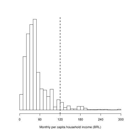
Figure 1. Histogram of the forcing variable: Monthly per capita household income (BRL) in 2008

In addition to the forcing variable, and thus, the eligibility status, for each family $i$ we observe: a binary outcome $Y_{i}$, equal to 1 if at least a leprosy case in family $i$ occurs in 2009, and $0$ otherwise, and a vector of $p=24$ covariates, $\mathbf{X}_{i}$, including information on the household structure, living and economic conditions of the family, and household head’s characteristics.

Table 2 presents some summary statistics for the sample, classified by assignment, $Z_{i}$, and Figure 2 shows leprosy rate (per mil) as a function of monthly per capita household income. As we can see in Table 2, there are systematic differences in background characteristics between eligible and ineligible families. Eligible families are on average younger and larger than ineligible families; they comprise a larger number of children and are in worse living and economic conditions than ineligible families. Moreover, the proportion of unemployed household heads is higher for eligible families than for ineligible families. The overall leprosy rate is $2.80\permil$, and it is slightly higher among eligible families than among ineligible families: $2.80\permil$ versus $2.72\permil$. Although leprosy is a rare outcome, making it difficult a graphical analysis of the outcome by forcing variable, there is some evidence that there is a discontinuity at the threshold (see Figure 2). See Section 6 for a discussion on this discontinuity.

Table 2. Bolsa Família study: Summary Statistics

$$\begin{array}[]{l rrr}\hline\cr&\hbox{Grand}&\lx@intercol\hfil\hbox{Means}\hfil\lx@intercol\\ \hbox{Variable}&\hbox{Means}&Z_{i}=0&Z_{i}=1\\ \lx@intercol\hfil\hbox{(Sample size)}\lx@intercol&(147\,399)&(9\,179)&(138\,220)\\ \hline\cr\vspace{-0.3cm}\\ \lx@intercol\hbox{{Household structure}}\hfil\lx@intercol\\ \vspace{-0.4cm}\\ \hbox{Min age}&10.93&19.97&10.32\\ \hbox{Mean age}&22.60&33.26&21.89\\ \hbox{Household size}&2.99&2.58&3.02\\ \hbox{N. Children}&1.34&0.72&1.38\\ \hbox{N. Adults}&1.60&1.55&1.60\\ \hbox{Children not at school}&0.04&0.02&0.04\\ \hbox{Presence of weak people}&0.22&0.16&0.23\\ \vspace{-0.3cm}\\ \lx@intercol\hbox{{Living and economic conditions}}\hfil\lx@intercol\\ \vspace{-0.4cm}\\ \hbox{Rural}&0.39&0.22&0.40\\ \hbox{Apartment}&0.95&0.96&0.95\\ \hbox{Home ownership: Homeowner}&0.59&0.67&0.58\\ \hbox{No rooms pc}&1.60&2.04&1.57\\ \hbox{House of bricks/row dirt }&0.91&0.95&0.91\\ \hbox{Water treatment}&0.79&0.85&0.78\\ \hbox{Water supply}&0.63&0.77&0.63\\ \hbox{Lighting}&0.79&0.91&0.79\\ \hbox{Bathroom fixture}&0.61&0.47&0.62\\ \hbox{Waste treatment}&0.64&0.81&0.63\\ \hbox{Zero PC expenditure}&0.21&0.16&0.22\\ \hbox{Log PC expenditure}&2.95&3.91&2.89\\ \hbox{Other programs}&0.06&0.06&0.06\\ \vspace{-0.3cm}\\ \lx@intercol\hbox{{Household head's characteristics}}\hfil\lx@intercol\\ \vspace{-0.4cm}\\ \hbox{Male}&0.86&0.83&0.87\\ \hbox{Race: Hispanic}&0.88&0.86&0.88\\ \hbox{Primary/Middle Education}&0.47&0.45&0.47\\ \hbox{Occupation: Unemployed}&0.49&0.37&0.49\\ \vspace{-0.3cm}\\ \lx@intercol\hbox{{Outcome variable}}\hfil\lx@intercol\\ \vspace{-0.4cm}\\ \hbox{Leprosy }(\permil)&2.80&2.72&2.80\\ \hline\cr\end{array}$$

Figure 2. Leprosy rate (per mil) as a function of the forcing variable (monthly per capita household income)

4. The Brazil’s Bolsa Família RD Design as Local Randomized Experiment

In RD designs under the local randomization framework, the forcing variable is stochastic and can be seen as the assignment variable. Therefore, under the potential outcomes approach (Rubin, 1974, 1978), potential outcomes need to be defined as function of the forcing variable. Throughout, we will maintain the common Stable Unit Treatment Value Assumption (SUTVA; Rubin, 1980), which implies that there is no interference, in the sense that the potential leprosy outcomes for a family cannot be affected by the value of monthly per capita household income (and thus, by the eligibility status) of other families. Under this assumption, we let $Y_{i}({s})$ denote the potential leprosy status that would be observed for the $i-$th family under a monthly per capita income equal to ${s}\in\mathbb{R}_{+}$.

The local randomization framework we adopt is based on three key assumptions, that we now introduce and discuss in the context of the Bolsa Família study.

The first assumption is a local overlap assumption: it requires that there exists at least a subpopulation around the threshold comprising families for which an overlap assumption holds, namely, families who have a probability of having a value of monthly per capita income falling on both sides of the threshold sufficiently far away from both zero and one. Formally,

Assumption 1.

(Local Overlap). There exists a subset of units, $\mathcal{U}_{s_{0}}\subseteq\mathcal{U}$, such that for each $i\in\mathcal{U}_{s_{0}}$, $\Pr(S_{i}\leq s_{0})>\epsilon$ and $\Pr(S_{i}>s_{0})>\epsilon$ for some sufficiently large $\epsilon>0$

Assumption 1 implies that families belonging to a subpopulation $\mathcal{U}_{s_{0}}$ have a non-zero marginal probability of being eligible to receive Bolsa Família benefits: $0<\Pr(Z_{i}=1)<1$ for all $i\in\mathcal{U}_{s_{0}}$. Assumption 1 is a local overlap assumption in the sense that it only applies to a subpopulation $\mathcal{U}_{s_{0}}$.

For families belonging to a subpopulation $\mathcal{U}_{s_{0}}$ we also adopt a modified Stable Unit Treatment Value Assumption (SUTVA; Rubin, 1980) specific to RD settings:

Assumption 2.

(Local RD-SUTVA). For each $i\in\mathcal{U}_{s_{0}}$, consider two eligibility statuses $z^{{}^{\prime}}=\mathbf{1}(S_{i}=s^{\prime}\leq s_{0})$ and $z^{{}^{\prime\prime}}=\mathbf{1}(S_{i}=s^{{}^{\prime\prime}}\leq s_{0})$, with possibly $s^{{}^{\prime}}\neq s^{{}^{\prime\prime}}$. $\hbox{If }z^{{}^{\prime}}=z^{{}^{\prime\prime}}\hbox{ then }Y_{i}({s}^{{}^{\prime}})=Y_{i}({s}^{{}^{\prime\prime}})$

Assumption 2 implies that the potential leprosy outcomes depend on monthly per capita household income solely through the eligibility status, $Z_{i}$, but not directly, so that, values of monthly per capita household income leading to the same eligibility status define the same potential leprosy outcome. Assumption 2 allows us to write $Y_{i}({s})$ as $Y_{i}(z)$ for each unit $i\in\mathcal{U}_{s_{0}}$, and thus, under local RD-SUTVA for each family $i$ within $\mathcal{U}_{s_{0}}$ there exist only two potential outcomes, $Y_{i}(0)$ and $Y_{i}(1)$: they are the values of the leprosy indicator if family $i$ had a value of monthly per capita household income falling above and below the threshold of $s_{0}=120$ BRL, respectively.

Under local overlap and local RD-SUTVA (Assumptions 1 and 2), causal effects are defined as comparisons of these two potential outcomes for a common set of units in the subpopulation $\mathcal{U}_{s_{0}}$. They are local causal effects in that they are causal effects for units belonging to a subpopulation $\mathcal{U}_{s_{0}}$. For our Bolsa Família study, we focus on the finite sample causal relative risk:

(1) $$RR_{\mathcal{U}_{s_{0}}}\equiv\dfrac{\sum_{i:i\in\mathcal{U}_{s_{0}}}Y_{i}(1)\Big{/}N_{\mathcal{U}_{s_{0}}}}{\sum_{i:i\in\mathcal{U}_{s_{0}}}Y_{i}(0)\Big{/}N_{\mathcal{U}_{s_{0}}}}$$

where $N_{\mathcal{U}_{s_{0}}}$ is the number of units in $\mathcal{U}_{s_{0}}$. For rare outcomes, such as leprosy, the causal relative risk is generally more informative than the causal risk difference.

Statistical inference for causal effects requires the specification of an assignment mechanism, which describes the probability of any vector of assignments, as a function of all covariates and of all potential outcomes. In our local randomization approach to RD design, we formalize the concept of an RD design as a local randomized experiment invoking the following assumption:

Assumption 3.

Local Unconfondedness. For each $i\in\mathcal{U}_{s_{0}}$,

$$\Pr\left(S_{i}\mid Y_{i}(0),Y_{i}(1),\mathbf{X}_{i}\right)=\Pr\left(S_{i}\mid\mathbf{X}_{i}\right).$$

Assumption 3 implies that for each family $i\in\mathcal{U}_{s_{0}}$,

$$\Pr\left(S_{i}\leq s_{0}\mid Y_{i}(0),Y_{i}(1),\mathbf{X}_{i}\right)=\Pr\left(S_{i}\leq s_{0}\mid\mathbf{X}_{i}\right)=\Pr\left(Z_{i}=1\mid\mathbf{X}_{i}\right),$$

which amounts to state that within the subpopulation $\mathcal{U}_{s_{0}}$, families with the same values of the covariates, $\mathbf{X}_{i}$, have the same probability of being observed under a specific value of the forcing variable, and, in turn, of being eligible or not for the Bolsa Família program. That is, in $\mathcal{U}_{s_{0}}$ eligibility is as good as random conditional on covariates, and does not depend on endogenous factors.

Under Assumptions 1-3, the causal estimand in Equation (1) is identified from the observed data. Formally, under Assumptions 1-3, for units in the subpopulation $\mathcal{U}_{s_{0}}$, we have

$$\Pr\left(Y_{i}(z)=1\mid i\in\mathcal{U}_{s_{0}}\right) = \mathbb{E}\left[Y_{i}(z)\mid i\in\mathcal{U}_{s_{0}}\right]$$

$$= \mathbb{E}_{X}\left[\mathbb{E}\left[Y_{i}(z)\mid\mathbf{X}_{i};i\in\mathcal{U}_{s_{0}}\right]\right]$$

$$= \mathbb{E}_{X}\left[\mathbb{E}\left[Y_{i}(z)\mid\mathbf{X}_{i},Z_{i}=z;i\in\mathcal{U}_{s_{0}}\right]\right]$$

$$= \mathbb{E}_{X}\left[\mathbb{E}\left[Y^{obs}_{i}\mid\mathbf{X}_{i},Z_{i}=z;i\in\mathcal{U}_{s_{0}}\right]\right]$$

where the first equation holds by definition, the second equality follows from the law of iterated expectation, the third equation follows from Assumption 3, and the last equality follows from Assumption 2. Therefore, let $\mathcal{X}$ denote the empirical support of $\mathbf{X}_{i}$, namely, the set of the observed values of the covariates, $\mathbf{X}_{i}$. Then, for $z=0,1$, the following equality holds:

(2) $$\qquad\dfrac{1}{N_{\mathcal{U}_{s_{0}}}}\sum_{i:i\in\mathcal{U}_{s_{0}}}Y_{i}(z)=\sum_{\mathbf{x}\in\mathcal{X}}\dfrac{1}{\sum_{i:i\in\mathcal{U}_{s_{0}}}\mathbf{1}\{\mathbf{X}_{i}=\mathbf{x}\}\mathbf{1}\{Z_{i}=z\}}\sum_{i:i\in\mathcal{U}_{s_{0}}}Y^{obs}_{i}\mathbf{1}\{\mathbf{X}_{i}=\mathbf{x}\}\mathbf{1}\{Z_{i}=z\}.$$

In the presence of a large number of covariates, possibly including continuous covariates, estimators of the causal relative risk based on Equation (2) are typically non-satisfactory. The Bayesian model-based approach allows us to easily adjust for covariates.

Assumptions 1-3, which we refer to as the RD assumptions throughout the paper, deserve some further discussion, that also clarifies similarities and differences between our local randomization approach to RD designs and the alternative local randomization approaches that have been proposed in the literature. Our approach closely follows Li et al., (2015) and Mattei and Mealli, (2016), but we make a weaker local unconfoundedness assumption: Li et al., (2015) and Mattei and Mealli, (2016) assume that the forcing variable and the potential outcomes are unconditionally independent, rather than conditionally independent given the covariates. Branson and Mealli, (2019) adopt a similar approach, but characterize the assignment mechanism assuming that the assignment indicator, $Z_{i}$, rather than, the forcing variable, $S_{i}$, is independent of the potential outcomes given the covariates. Their assumptions are slightly weaker than our Assumption 3, because the assignment indicator, $Z_{i}$, only depends on $S_{i}$ through the cutoff rule.

Moreover, our approach presents important differences with the methodological framework developed by Cattaneo et al., (2015); Sales and Hansen, (2020) and Eckles et al., (2020). The “local randomization” framework proposed by Cattaneo et al., (2015) relies on the assumption that there exists a subpopulation of units where the following two conditions hold: $(i)$ the marginal distributions of the forcing variable are the same for all units inside that subpopulation; and $(ii)$ potential outcomes depend on the values of the forcing variable only through treatment indicators. This assumption does not actually define an assignment mechanism as the conditional probability of the assignment variable given covariates and potential outcomes, but it mixes up the concept of random assignment, implying that the values of the forcing variable can be considered “as good as randomly assigned,” and SUTVA, and thus, the definition of potential outcomes, requiring that potential outcomes depend on the values of the forcing variable only through the treatment assignment indicators. Sales and Hansen, (2020) introduce a “residual ignorability” assumption, which requires that the residual of a model of the outcome under control on the forcing variable is independent of treatment assignment status. Recently, Eckles et al., (2020) propose to attribute the stochasticity of the realized forcing variable to the stochasticity of a measurement error under the assumption of “exogeneity of the noise in the forcing variable.” This exogeneity assumption requires that the observed forcing variable and the potential outcomes are independent conditional on the latent true forcing variable. In some sense, the “residual ignorability” assumption introduced by Sales and Hansen, (2020) and the assumption of “exogeneity of the noise in the forcing variable” introduced by Eckles et al., (2020) are relatively similar in that they both invoke ignorability of error terms. At first glance, the assumption of “exogeneity of the noise in the forcing variable” and our local unconfoundedness assumption might seem closely related, but they are indeed different assumptions with different inferential implications. Exogeneity of the noise in the forcing variable is a type of latent unconfoundedness, because unconfoundedness is assumed to hold conditional on a latent variable, of which the forcing variable is a noisy measure. Under this assumption average causal effects at the threshold can be identified and estimated. Therefore, exogeneity of the noise in the forcing variable can be viewed as an alternative to continuity assumptions, when the focus is on identifying and estimating average causal effects at the threshold, rather than causal effects for subpopulations of units with values of the forcing variable far away from the threshold. In our framework, local unconfoundedness amounts to assuming that in the subpopulation $\mathcal{U}_{s_{0}}$, for families with the same values of the covariates, truly exogenous factors determine whether the realized value of the forcing variable falls above or below the threshold. This exogeneity implies that if there were measurement error in the forcing variable, the latent true forcing variable would be well described by the observed covariates for the subpopulation $\mathcal{U}_{s_{0}}$, so that, for families in the subpopulation $\mathcal{U}_{s_{0}}$, the conditional distribution of the latent true forcing variable given the covariates would be the same in the two groups defined by the treatment assignment indicator. It is not at all obvious which of the two assumptions, our local unconfoundedness and the exogeneity of the noise in Eckles et al., (2020), is more or less plausible in real settings, given that they are not nested and that they allow the identification of different causal estimands.

5. Selection of Subpopulations $\mathcal{U}_{s_{0}}$

Assumptions 1-3 implies that if we knew at least one subpopulation $\mathcal{U}_{s_{0}}$ where these RD assumptions hold, we could draw inference on causal effects for that subpopulation using standard methods for analyzing randomized experiments or regular observational studies. Unfortunately, in practice, true subpopulations where the RD assumptions hold are usually unknown. Therefore a critical issue of the approach is how to choose subpopulations $\mathcal{U}_{s_{0}}$ for which we can draw valid causal inference.

5.1. Selection of Subpopulations $\mathcal{U}_{s_{0}}$: State of the Art.

The existing approaches in the literature on the local randomization framework deal with this issue by exploiting the implications of the assumptions on the assignment mechanism. Under the assumption that suitable subpopulations have a rectangular shape, comprising units with a realized value of the forcing variable falling in a symmetric interval around the threshold: $\mathcal{U}_{s_{0}}=\{i:S_{i}\in[s_{0}-h,s_{0}+h]\}$, Cattaneo et al., (2015); Li et al., (2015); Mattei and Mealli, (2016); Licari and Mattei, (2020); Branson and Mealli, (2019) propose to use falsification tests for selecting the bandwidth $h$ that exploits the local nature of the invoked randomization / unconfoundedness assumption. A local randomization / unconfoundedness assumption, such as our Assumption 3, holds for a subset of units, but may not hold in general for other units. Therefore, under local randomization / unconfoundedness assumption, covariates that do not enter the assignment mechanism, should be well balanced in the two subsamples defined by $Z_{i}$ in $\mathcal{U}_{s_{0}}$, and thus any test of the null hypothesis of no difference in the distribution (or mean) of covariates between eligible and ineligible should fail to reject the null. Cattaneo et al., (2015) and Branson and Mealli, (2019) propose to use randomization-based falsification tests. Branson and Mealli, (2019) show that different windows around the cutoff may be selected depending on the type of assignment mechanism a researcher is willing to posit. Li et al., (2015) and Licari and Mattei, (2020) propose a Bayesian model-based hierarchical approach accounting for the problem of multiplicities to test if the covariate mean differences between eligible and ineligible are significantly different from zero. The falsification test approach is not suitable for the Bolsa Família study, where the large sample size leads to reject the null hypothesis of covariates’ balancing even for subpopulations defined by very small neighbors around the threshold.

The falsification test approach is relatively simple to implement, but two important pitfalls threaten it. First, it generally relies on the assumption that suitable subpopulations have a rectangular shape. Although this assumption offers computational advantages, restricting the set of candidate subpopulations, it may be without grounds or be difficult to justify from a substantive perspective. Second, causal inference is drawn conditionally on the results of the falsification tests: the uncertainty about a selected subpopulation is never incorporated in the inferences for the causal effects of interest.

Under a local unconfoundedness assumption, Keele et al., (2015) propose to select a subpopulation conditioning on observables and the discontinuity using a penalized matching framework, where the distance between eligible and ineligible observations with respect to the forcing variable is minimized penalizing matching units too faraway while preserving balance in pretreatment covariates. A critical issue of this approach is the choice of the penalty term: the selected subpopulation critically depends on the penalty given to the distance in the forcing variable between eligible and ineligible observations. Recently, Ricciardi et al., (2020) propose to conduct the analyses on a subset of units belonging to balanced and homogeneous clusters, identified using a Dirichlet process mixture model, where clusters are defined to be balanced if they comprise a sufficiently large number of units on both sides of the threshold and to be homogeneous if they comprise observations that are similar to one another with respect to the covariates. It is not fully explicit what implications this procedure has on the assignment mechanism. These methods do not require any assumption on the shape of the subpopulations, but causal inference is again conducted without directly accounting for the uncertainty about a selected subpopulation, as with the falsification test approach.

Missing to account for the uncertainty about the selection of suitable subpopulations is an important drawback of all existing methods to the analysis of RD designs, where focus is on drawing causal inference for either one subpopulation or for more than one subpopulation separately.

5.2. A Bayesian Model-Based Finite Mixture Approach to the Selection of Subpopulations $\mathcal{U}_{s_{0}}$.

The data challenges raised by the Bolsa Família study and the pitfalls of the existing approaches prompted us to develop a new approach to the selection of suitable subpopulations in RD designs. We propose a Bayesian model-based finite mixture approach to clustering to classify observations into subpopulations where the RD assumptions hold and do not hold on the basis of the observed data.

The key insight underlying our approach is to view the families in the Bolsa Família study as coming from three subpopulations:

1. the subpopulation of families with a realized value of forcing variable (monthly per capita household income) falling in some neighborhood, ${\mathcal{I}}_{s_{0}}$, around the threshold, $s_{0}$, where the RD assumptions hold: ${\mathcal{U}_{s_{0}}=\{i:S_{i}\in{\mathcal{I}}_{s_{0}}\}}$;

2. the subpopulation of families who do not belong to $\mathcal{U}_{s_{0}}$ for which some of the RD assumptions may fail to hold, and have a realized value of the forcing variable below the threshold, $s_{0}$: $\mathcal{U}_{s_{0}}^{-}=\{i:S_{i}\notin{\mathcal{I}}_{s_{0}}\hbox{ and }S_{i}<s_{0}\}$;

3. the subpopulation of families who do not belong to $\mathcal{U}_{s_{0}}$ for which some of the RD assumptions may fail to hold, and have a realized value of the forcing variable above the threshold, $s_{0}$: $\mathcal{U}_{s_{0}}^{+}=\{i:S_{i}\notin{\mathcal{I}}_{s_{0}}\hbox{ and }S_{i}>s_{0}\}$;

The subpopulations $\mathcal{U}_{s_{0}}$, $\mathcal{U}_{s_{0}}^{+}$ and $\mathcal{U}_{s_{0}}^{-}$ define a partition of the whole population, $\mathcal{U}$: $\mathcal{U}=\mathcal{U}_{s_{0}}\cup\mathcal{U}_{s_{0}}^{-}\cup\mathcal{U}_{s_{0}}^{+}$, and $\mathcal{U}_{s_{0}}\cap\mathcal{U}_{s_{0}}^{-}=\mathcal{U}_{s_{0}}\cap\mathcal{U}_{s_{0}}^{+}=\mathcal{U}_{s_{0}}^{-}\cap\mathcal{U}_{s_{0}}^{+}=\emptyset$, and thus, each family in the study must belong to one of three subpopulations. A clear definition of the characteristics of each subpopulation is key to our approach. For families who belong to $\mathcal{U}_{s_{0}}$ the RD assumptions must hold, whereas for families who belong to $\mathcal{U}_{s_{0}}^{-}\cup\mathcal{U}_{s_{0}}^{+}$, some of the RD assumptions may fail to hold. Specifically, for families who do not belong to $\mathcal{U}_{s_{0}}$, the local overlap assumption may be untenable, in the sense that those families may have a zero probability of being assigned to either eligibility statutes and/or there may be a relationship between the forcing variable and potential outcomes, monthly per capita household income and presence of leprosy cases in the family, implying that either local RD-SUTVA (Assumption 2) or local unconfoundedness (Assumption 3) is questionable. For families in $\mathcal{U}_{s_{0}}^{-}\cup\mathcal{U}_{s_{0}}^{+}$, the failure of local RD-SUTVA affects the definition of the potential outcomes, which must be indexed by the forcing variable; and the failure of local unconfoundedness implies that the assignment mechanism depends on the potential outcomes.

We use these features characterizing the three subpopulations as input for our Bayesian model-based finite mixture approach for classifying families into the three subpopulations. Specifically, we view the joint conditional distribution of the forcing variable and the potential outcomes given the observed covariates as a three-component finite mixture distribution with unknown mixture proportions (e.g., Titterington et al., 1985; McLachlan and Basford, 1988). The three components correspond to the three subpopulations, $\mathcal{U}_{s_{0}}$, $\mathcal{U}_{s_{0}}^{+}$, and $\mathcal{U}_{s_{0}}^{-}$: we characterize them to match their definition with respect to the RD assumptions and the value of the forcing variable falling below or above the threshold. Formally, we specify the following mixture model:

$$p\left(S_{i},\{Y_{i}({s})\}_{{s}\in\mathbb{R}_{+}}\mid\mathbf{X}_{i};\bm{\theta}\right)$$

$$= \pi_{i}(\mathcal{U}_{s_{0}};\bm{\theta})\,p(S_{i},\{Y_{i}({s})\}_{{s}\in\mathbb{R}_{+}})\mid\mathbf{X}_{i},i\in\mathcal{U}_{s_{0}};\bm{\theta})+$$

$$\pi_{i}(\mathcal{U}_{s_{0}}^{-};\bm{\theta})\,p(S_{i},\{Y_{i}({s})\}_{{s}\in\mathbb{R}_{+}}\mid\mathbf{X}_{i};i\in\mathcal{U}_{s_{0}}^{-};\bm{\theta})+$$

$$\pi_{i}(\mathcal{U}_{s_{0}}^{+};\bm{\theta})\,p(S_{i},\{Y_{i}({s})\}_{{s}\in\mathbb{R}_{+}}\mid\mathbf{X}_{i},i\in\mathcal{U}_{s_{0}}^{+};\bm{\theta})$$

$$= \pi_{i}(\mathcal{U}_{s_{0}};\bm{\alpha})\,p(S_{i}\mid\mathbf{X}_{i},i\in\mathcal{U}_{s_{0}};\bm{\eta})\,p(Y_{i}(0),Y_{i}(1)\mid\mathbf{X}_{i},i\in\mathcal{U}_{s_{0}};\bm{\gamma})+$$

$$\pi_{i}(\mathcal{U}_{s_{0}}^{-};\bm{\alpha})\,p(S_{i}\mid\mathbf{X}_{i};i\in\mathcal{U}_{s_{0}}^{-};\bm{\eta}^{-})\,p(\{Y_{i}(s)\}_{s\in\mathbb{R}_{+}}\mid S_{i},\mathbf{X}_{i};i\in\mathcal{U}_{s_{0}}^{-};\bm{\gamma}^{-})+$$

$$\pi_{i}(\mathcal{U}_{s_{0}}^{+};\bm{\alpha})\,p(S_{i}\mid\mathbf{X}_{i},i\in\mathcal{U}_{s_{0}}^{+};\bm{\eta}^{+})\,p(\{Y_{i}(s)\}_{s\in\mathbb{R}_{+}}\mid S_{i},\mathbf{X}_{i},i\in\mathcal{U}_{s_{0}}^{+};\bm{\gamma}^{+})$$

where $\pi_{i}(\mathcal{U}_{s_{0}};\bm{\alpha})=Pr(i\in\mathcal{U}_{s_{0}}\mid\mathbf{X}_{i};\bm{\alpha})\geq 0$, $\pi_{i}(\mathcal{U}_{s_{0}}^{-};\bm{\alpha})=Pr(i\in\mathcal{U}_{s_{0}}^{-}\mid\mathbf{X}_{i};\bm{\alpha})\geq 0$ and $\pi_{i}(\mathcal{U}_{s_{0}}^{+};\bm{\alpha})=Pr(i\in\mathcal{U}_{s_{0}}^{+}\mid\mathbf{X}_{i};\bm{\alpha})\geq 0$ are the mixing probabilities, with $\pi_{i}(\mathcal{U}_{s_{0}}^{-};\bm{\alpha})+\pi_{i}(\mathcal{U}_{s_{0}};\bm{\alpha})+\pi_{i}(\mathcal{U}_{s_{0}}^{+};\bm{\alpha})=1$; $(\bm{\eta}^{-},\bm{\gamma}^{-})$, $(\bm{\eta},\bm{\gamma})$ and $(\bm{\eta}^{+},\bm{\gamma}^{+})$ are parameter vectors defining each mixture component, and $\bm{\theta}=\left(\bm{\alpha},\bm{\eta}^{-},\bm{\gamma}^{-},\bm{\eta},\bm{\gamma},\bm{\eta}^{+},\bm{\gamma}^{+}\right)$ is the complete set of parameters specifying the mixture.

Equation (5.2) formally describes the joint distribution of the forcing variable, $S_{i}$, and the potential outcomes, $\{Y_{i}({s})\}_{{s}\in\mathbb{R}_{+}}$, as a three mixture distribution, and Equation (5.2) follows from imposing the RD assumptions for units in $\mathcal{U}_{s_{0}}$ and allowing for violations of those assumptions for units who do not belong to $\mathcal{U}_{s_{0}}$. Specifically, the mixture component corresponding to the subpopulation $\mathcal{U}_{s_{0}}$ in Equation (5.2) is specified to reflect the RD assumptions: under local overlap (Assumption 1), first, local RD-SUTVA (Assumption 2) implies that for each family in $\mathcal{U}_{s_{0}}$ there exist only two potential outcomes, $Y_{i}(0)$ and $Y_{i}(1)$, the two potential outcomes corresponding to the two eligibility statues; second, local unconfoundedness (Assumption 3) implies that the forcing variable and the potential outcomes are conditionally independent given the covariates, so that, conditional on the observed covariates, the joint distribution of the forcing variable and the potential outcomes factorizes into the product of the marginal distribution of the forcing variable and the marginal distribution of potential outcomes.

It is worth noting that our model specification does not impose any constraint on the distribution of the forcing variable; the local overlap assumption (Assumption 1) is not used as a classification criterion. We are implicitly assuming that the local overlap assumption (Assumption 1) holds in the subpopulation $\mathcal{U}_{s_{0}}$ and we allow that the probability of being assigned to either eligibility statues may take any value between zero and one, including zero and one, for families in $\mathcal{U}_{s_{0}}^{-}$ and $\mathcal{U}_{s_{0}}^{+}$.

The specification of the mixture components describing the joint conditional distribution of the forcing variable and the potential outcomes in the subpopulations $\mathcal{U}_{s_{0}}^{-}$ and $\mathcal{U}_{s_{0}}^{+}$ reflects possible violations of local RD-SUTVA and/or local unconfoundedness: potential outcomes are defined as a function of the vector of values of the forcing variable; and the forcing variable and the potential outcomes may be not independent, even conditional on the covariates. A possible threat to unconfoundedness is the presence of some manipulation of the forcing variable; because our proposed approach is able to leave out units for whom unconfoundedness does not hold, it should also lead to more robust evidence against the presence of manipulation. We will return to this when discussing our case study in Section 6.

After specifying a parametric form for each component probability distribution of the mixture, we propose to use a Bayesian approach to fit the mixture model. Posterior inference of the parameters can be obtained using Gibbs sampling with a data augmentation step to impute the missing subpopulation membership for each unit Diebolt and Robert, (1994); Richardson and Green, (1997). Specifically, we derive the posterior distribution of the causal estimand in Equation (1) using an MCMC algorithm with data augmentation (Tanner and Wong, 1987), where at each iteration $\ell$, $\ell=1,\ldots,L$, of the MCMC algorithm: $(1)$ we impute the missing subpopulation membership for each family using a data augmentation step; $(2)$ we update the model parameters using Gibbs sampling methods; and $(3)$ for each family classified in $\mathcal{U}_{s_{0}}^{\ell}$, we draw the missing potential outcome, $Y_{i}^{\ell}=Z_{i}Y_{i}(0)+(1-Z_{i})Y_{i}(1)$, from its posterior predictive distribution and calculate the causal relative risk ratio:

$$RR^{\ell}_{\mathcal{U}_{s_{0}}}=\dfrac{\sum_{i:i\in\mathcal{U}_{s_{0}}^{\ell}}[Z_{i}Y_{i}+(1-Z_{i})Y_{i}^{\ell}(1)]\Big{/}N_{\mathcal{U}_{s_{0}}^{\ell}}}{\sum_{i:i\in\mathcal{U}_{s_{0}}^{\ell}}[(1-Z_{i})Y_{i}+Z_{i}Y_{i}^{\ell}(0)]\Big{/}N_{\mathcal{U}_{s_{0}}^{\ell}}},$$

where $Y_{i}=Z_{i}Y_{i}(1)+(1-Z_{i})Y_{i}(0)$ is the observed potential outcome. See e-Appendix A for further details.

In this framework, each unit’s contribution to the posterior distribution of the causal estimand of interest differs depending on the posterior probability of that unit belonging to the subpopulation $\mathcal{U}_{s_{0}}$. Observations with a higher posterior probability of meeting the RD assumptions (as determined by the relationship between the outcome and the forcing variable conditional on the covariates) will be included more often in $\mathcal{U}_{s_{0}}$ and will contribute more information to the final posterior inference. Observations exhibiting characteristics that may undercut the plausibility of the RD assumptions will contribute less to the inference for causal effects.

5.3. Specification of the Finite Mixture Model in the Bolsa Família Study.

In the Bolsa Família study, to model the mixing probabilities we adopt two conditional probit models, defined using latent variables $G^{\ast}_{i}(-)$ and $G^{\ast}_{i}(+)$, for whether family $i$ belongs to the subpopulation $\mathcal{U}_{s_{0}}^{-}$ or $\mathcal{U}_{s_{0}}^{+}$:

$$\pi_{i}(\mathcal{U}_{s_{0}}^{-})=\Pr(G^{\ast}_{i}(-)\leq 0)\qquad\hbox{and}\qquad\pi_{i}(\mathcal{U}_{s_{0}}^{+})=\Pr(G^{\ast}_{i}(-)>0\,\mathrm{and}\,G^{\ast}_{i}(+)\leq 0)$$

where

$$G^{\ast}_{i}(-)=\alpha_{0}^{-}+\mathbf{X}_{i}^{\prime}\bm{\alpha}^{-}_{X}+\epsilon_{i}^{-}\qquad\text{and}\qquad G^{\ast}_{i}(+)=\alpha_{0}^{+}+\mathbf{X}_{i}^{\prime}\bm{\alpha}^{+}_{X}+\epsilon_{i}^{+}$$

with $\epsilon_{i}^{-}\sim N(0,1)$ and $\epsilon_{i}^{+}\sim N(0,1)$, independently. Clearly $\pi_{i}(\mathcal{U}_{s_{0}})=1-\pi_{i}(\mathcal{U}_{s_{0}}^{-})-\pi_{i}(\mathcal{U}_{s_{0}}^{+})$. For the forcing variable, we specify log-Normal models with the mean linear in the covariates with subpopulation-specific parameters and with subpopulation-specific variances. We specify log-Normal models for a transformation of the forcing variable: $\tilde{S}_{i}=\sqrt[10]{S_{i}/s_{0}}$, so that $\log(\tilde{S}_{i})=[\log(S_{i})-\log(s_{0})]/10$. Therefore, our model specification implies that Normal distributions are used to model the distance on log scale of the forcing variable from the threshold, re-scaled by a factor of 10. Formally,

$$\log(\tilde{S}_{i})\mid\mathbf{X}_{i},i\in\mathcal{U}_{s_{0}}^{-} \sim N\left(\beta_{0}^{-}+\mathbf{X}_{i}^{\prime}\bm{\beta}^{-}_{X};\sigma^{2}_{-}\right)$$

$$\log(\tilde{S}_{i})\mid\mathbf{X}_{i},i\in\mathcal{U}_{s_{0}}^{+} \sim N\left(\beta_{0}^{+}+\mathbf{X}_{i}^{\prime}\bm{\beta}^{+}_{X};\sigma^{2}_{+}\right)$$

$$\log(\tilde{S}_{i})\mid\mathbf{X}_{i},i\in\mathcal{U}_{s_{0}} \sim N\left(\beta_{0}+\mathbf{X}_{i}^{\prime}\bm{\beta}_{X};\sigma^{2}\right)$$

Because our outcome is dichotomous, we assume that the marginal distributions of the outcome take the form of generalized linear Bernoulli models with a probit link:

$$\Pr(Y_{i}(s)=1\mid S_{i}=s,\mathbf{X}_{i},i\in\mathcal{U}_{s_{0}}^{-}) = \Phi\left(\gamma_{0}^{-}+\log(\tilde{s})\gamma_{1}^{-}+\mathbf{X}_{i}^{\prime}\bm{\gamma}^{-}_{X}\right)$$

$$\Pr(Y_{i}(s)=1\mid S_{i}=s,\mathbf{X}_{i},i\in\mathcal{U}_{s_{0}}^{+}) = \Phi\left(\gamma_{0}^{+}+\log(\tilde{s})\gamma_{1}^{+}+\mathbf{X}_{i}^{\prime}\bm{\gamma}^{+}_{X}\right)$$

$${\Pr(Y_{i}(z)=1|\mathbf{X}_{i},i\in\mathcal{U}_{s_{0}})} {=} {\Phi\left(\gamma_{0,z}+\mathbf{X}_{i}^{\prime}\bm{\gamma}_{X,z}\right)\qquad z=0,1}$$

where $\Phi(\cdot)$ denotes the cumulative distribution function of a standard Normal distribution. For reasons of model performance, we model the dependence between the potential outcomes and the forcing variable in the subpopulations $\mathcal{U}_{s_{0}}^{-}$ and $\mathcal{U}_{s_{0}}^{+}$, using the logarithm of the transformation of the forcing variable defined above: $\log(\tilde{s})=\log(\!\sqrt[10]{s/s_{0}})$. For parsimony and for gaining information across groups, we impose a priori equality of the slope coefficients in the outcome regressions: $\bm{\gamma}_{X}^{-}=\bm{\gamma}_{X}^{+}=\bm{\gamma}_{X,z=0}=\bm{\gamma}_{X,z=1}\equiv\bm{\gamma}_{X}$.

Bayesian inference on finite sample causal estimands for a subset of units in the study, such as the local causal relative risk in Equation (1) we are interested in, follows from predictive Bayesian inference, and generally involves parameters describing the association between potential outcomes (e.g. Imbens and Rubin, 1997, 2015). Nevertheless, the association parameters do not enter the likelihood function: because we never simultaneously observe all the potential outcomes for any unit, the data contain no information about the association between the potential outcomes. Therefore, the posterior distribution of the association parameters will be identical to its prior distribution if we assume that they are a priori independent of the other parameters. Throughout the paper, we assume that the unobserved potential outcomes are independent of the observed potential outcome conditional on the covariates and parameters, namely, we assume that $Y_{i}(0)$ and $Y_{i}(1)$ are conditionally independent for units in $\mathcal{U}_{s_{0}}$, and $Y_{i}(s)$, for $s\in\mathbb{R}_{+}$, are conditionally independent for units in either $\mathcal{U}_{s_{0}}^{-}$ or $\mathcal{U}_{s_{0}}^{+}$. Therefore, the above model assumptions completely specify the mixture model in Equation (5.2). The full parameter vector is $\bm{\theta}=\{(\alpha_{0}^{-},\bm{\alpha}^{-}_{X}),(\alpha_{0}^{+},\bm{\alpha}^{+}_{X}),$ $(\beta_{0}^{-},\bm{\beta}^{-}_{X},\sigma^{2}_{-}),$ $(\beta_{0}^{+},\bm{\beta}^{+}_{X},\sigma^{2}_{+}),$ $(\beta_{0},\bm{\beta}_{X},\sigma^{2}),$ $(\gamma_{0}^{-},\gamma_{1}^{-}),$ $(\gamma_{0}^{+},\gamma_{1}^{+}),$ $\gamma_{0,z=0},$ $\gamma_{0,z=1},$ $\bm{\gamma}_{X})\}$, which includes $6\times p+14=6\times 24+14=158$ parameters.

Bayesian inference is conducted under the assumption that parameters are a priori independent and using multivariate normal prior distributions for the regression coefficients and inverse-chi square distributions for the variances of the model for the forcing variable. Specifically, the prior distributions for the mixing probabilities are multivariate normal distributions with covariance-variance matrices equal to scalar matrices with equal-valued elements along the diagonal set at $1$. The mean vectors are vectors of zeros with the exception of the first element of the mean vector of the coefficients of the probit submodel for $\mathcal{U}_{s_{0}}^{-}$ membership which is set equal to $\Phi^{-1}(2/3)\sqrt{1+\overline{X}^{\prime}\overline{X}}$, where $\overline{X}$ is the mean vector of the covariates. These prior specifications result in approximately setting the prior probability of belonging to each subpopulations at 1/3 for each individual (see Figure 5(A)), which reflects our a priori ignorance about such probabilities. For the regression coefficients of the models for the outcome, we use as prior distributions multivariate normal distributions with mean vector zero and covariance-variance matrices equal to scalar matrices with equal-valued elements along the diagonal set at $1$. For the log-normal models of the forcing variable, we specify multivariate normal distributions with mean vector zero and scalar covariance-variance matrices with equal-valued elements along the diagonal set at $100$ for the regression coefficients and inverse chi-squared distributions with degrees of freedom set at $3$ and scale parameter set at $1/3$ for the variances (See e-Appendix A for details).

5.4. Accounting for the Uncertainty in $\mathcal{U}_{s_{0}}-$ Membership.

An appealing feature of our approach is that it can properly account for the uncertainty in the subpopulations for which we can draw valid causal inference, that is, for which the RD assumptions (Assumptions 1-3) hold. Our approach can be embedded in a broader perspective, which makes it a very flexible tool.

First, the proposed approach can be viewed as a Bayesian sensitivity analysis to the RD assumptions, in general, and to the local unconfoundedness assumption (Assumption 3), in particular. In this regard, it has similarities with the sensitivity analysis approach to unmeasured confounding in observational studies recently proposed by Bonvini and Kennedy, (2022). Specifically, Bonvini and Kennedy, (2022) proposes an approach to sensitivity analysis based on a mixture model for confounding, viewing the units in the sample as coming from a mixture of two distributions: a distribution where treatment assignment is unconfounded (conditional on the observed covariates), and a distribution for which the treatment assignment is arbitrarily confounded (even after conditioning on the observed covariates). Then, they use the mixing probability, namely the proportion of units for which the assignment mechanism is arbitrarily confounded, as a sensitivity parameter and derive sharp bounds on the average causal effects as a function of it. The proportion of confounded units, the sensitivity parameter, is unknown and so inferences on the average causal effects are drawn by varying it in a plausible range of values. In a sense, from a sensitivity analysis perspective, our approach can be construed as a stochastic version of the mixture model for confounding proposed by Bonvini and Kennedy, (2022): our approach, as Bayesian sensitivity analysis, does not require to vary the proportion of confounded units as a sensitivity parameter, but it stochastically selects observations in $\mathcal{U}_{s_{0}}$, for which unconfoundedness (above and beyond local overlap and local RD-SUTVA) holds. Ultimately, we regard membership in hypothetical subpopulations $\mathcal{U}_{s_{0}}$ as unknown for each observation, and derive the posterior distribution of the causal effect by marginalizing over the uncertainty in whether each observation is a member. Thus, the resulting posterior distribution of the causal effect, where the contribution of each unit depends on the posterior probability of that unit’s inclusion in $\mathcal{U}_{s_{0}}$, incorporates the uncertainty in $\mathcal{U}_{s_{0}}$ membership.

In this paper, we opt for a Bayesian approach to inference, and thus, we combine the “design” and “analysis” phases of the RD study. As an alternative, we can use the proposed approach as an innovative method to “design” an RD study that allows the selection of the subpopulation that can be used in the analysis phase and to account for its uncertainty. The key insight is that we can view the selection of the subpopulation $\mathcal{U}_{s_{0}}$ as a missing data problem, where membership is missing for each observation. Then, we can deal with this missing data issue using the proposed Bayesian model-based mixture approach to multiple impute subpopulation membership, that is, to fill in the missing subpopulation membership for each unit with a vector of $M>1$ plausible imputed values, creating a set of $M$ completed membership datasets. In the analysis phase, for each of the $M$ complete membership datasets, we can use units classified in the subpopulation $\mathcal{U}_{s_{0}}$ to draw inference on the causal effects of interest under either the local randomization framework or the traditional framework.

Under the local randomization framework, for each of the $M$ complete membership datasets, the RD assumptions – local overlap (Assumption 1), local RD-SUTVA (Assumption 2) and local unconfoundedness (Assumption 3) – are supposed to hold for units classified in the subpopulation $\mathcal{U}_{s_{0}}$, and thus, we can draw inference on the causal effects of interest for those units using any proper mode of causal inference under the treatment assignment mechanism described by the invoked local unconfoundedness assumption, including modes based only on the assignment mechanism (Fisherian and Neymanian modes of inference) and Bayesian model-based modes of inference Li et al., (2015); Mattei and Mealli, (2016); Branson and Mealli, (2019); Licari and Mattei, (2020).

Although the local randomization framework appears a natural choice, a traditional approach to the analysis of RD design can be also used. Under assumptions of continuity of conditional regression functions (or conditional distribution functions) of the outcomes given the forcing variable, we can use units in the subpopulation $\mathcal{U}_{s_{0}}$ to draw inference on the average causal effect at the threshold using, e.g., local-polynomial (non-)parametric regression methods. For each of the $M$ complete membership datasets, units classified in the subpopulation $\mathcal{U}_{s_{0}}$ can either be directly used as an “auxiliary” subset of units from which extrapolating information to the cutoff, or be viewed as a properly selected pool from which constructing the “auxiliary” subset of units through the choice of a bandwidth defining a smoothing window around the threshold, using data-driven methods Calonico et al., (2018) or Mean Square Error (MSE)-optimal criteria Imbens and Kalyanaraman, (2012); Calonico et al., (2014).

The $M$ complete-membership inferences can be easily combined to form one inference that appropriately reflects both sampling variability and missing $\mathcal{U}_{s_{0}}-$membership uncertainty. Let $\tau$ be the causal estimand of interest, for instance, the finite sample causal relative risk for the subpopulation $\mathcal{U}_{s_{0}}$, $\tau=RR_{\mathcal{U}_{s_{0}}}$ in the local randomization framework, or the average causal effect at the threshold, $s_{0}$, $\tau=\mathbb{E}[Y_{i}(1)-Y_{i}(0)\mid S_{i}=s_{0}]$, in the traditional framework. Let $\widehat{\tau}$ and $\widehat{V}$ be the complete-data membership estimators of $\tau$ and the sampling variance of $\widehat{\tau}$, respectively. Also, let $\widehat{\tau}_{m}$ and $\widehat{V}_{m}$, $m=1,\ldots,M$, be $M$ estimates of $\tau$ and their associated sampling variances, calculated from the $M$ completed membership datasets. The final point estimate of $\tau$ can be obtained by averaging together the the $M$ completed-membership estimates: $\widehat{\tau}_{\mathrm{MI}}=M^{-1}\sum_{\ell=1}^{M}\widehat{\tau}_{m}$. The variability associated with this estimate is $\widehat{\theta}_{\mathrm{MI}}$ is $W_{M}+\left(1+M^{-1}\right)B_{M}$, where $W_{M}=M^{-1}\sum_{m=1}^{M}\widehat{V}_{m}$ is the average within-imputation variance, $B_{M}=(M-1)^{-1}\sum_{m=1}^{M}\left(\widehat{\tau}_{m}-\widehat{\tau}_{\mathrm{MI}}\right)^{2}$ is the between-imputation variance, and the factor $\left(1+M^{-1}\right)$ reflects the fact that only a finite number of completed-membership estimates $\widehat{\tau}_{m}$, $m=1,\ldots,M$, are averaged together to obtain the final point estimate Rubin, (1987).

5.5. Simulation Study under Challenging Scenarios.

We conduct extensive simulation studies to investigate how our approach works even in challenging scenarios. The primary aim is to shed light on the sources of identification of the subpopulation membership; also a concern is whether our procedure is able to recognize that the subpopulation $\mathcal{U}_{s_{0}}$ is empty or whether, instead, it wrongly creates a “fake” subpopulation by selecting observations such that the dependency between the outcome and the forcing variable is broken.

In our Bayesian model-based finite mixture approach to clustering the covariates and the outcome model play a crucial role in classifying units into the three subpopulations, $\mathcal{U}_{s_{0}}$, $\mathcal{U}_{s_{0}}^{-}$, and $\mathcal{U}_{s_{0}}^{+}$. Because units belonging to a subpopulation $\mathcal{U}_{s_{0}}$ should have characteristics such that their probability to fall on either side of the threshold is sufficiently far away from zero and one, $\mathcal{U}_{s_{0}}$ should comprise treated and control units (below and above the cutoff) with similar background characteristics. For $\mathcal{U}_{s_{0}}$, local-SUTVA (Assumption 2) and local unconfoundedness (Assumption 3) hold, and thus, potential outcomes and forcing variable are structurally and statistically independent for units belonging to $\mathcal{U}_{s_{0}}$. For units in $\mathcal{U}_{s_{0}}^{-}$ or $\mathcal{U}_{s_{0}}^{+}$, local-SUTVA or local unconfoundedness does not hold, implying that potential outcomes depend on the forcing variable. Our simulation results confirm and highlight that the covariates and the outcome model play a key role in classifying units into the three subpopulations. In extreme scenarios, where there are no units in $\mathcal{U}_{s_{0}}$, i.e., $\mathcal{U}_{s_{0}}$ is empty, simulations show that our approach works very well.

See e-Appendix D for a further description of the simulation results.

6. Design and Analysis of the Bolsa Família Study

We apply the Bayesian model-based finite mixture approach described in Section 5 for both the design and the analysis of the Bolsa Família program to assess its effect on leprosy incidence.

A preliminary discussion is deserved. In RD designs, concerns about the validity of the RD approach may arise if the forcing variable is susceptible to manipulation. Because Bolsa Família applicants know the eligibility criteria, there is a concern that they might attempt to report a lower income in order to end up below the threshold and receive the Bolsa Família benefits. If this is the case, the eligible families just below the threshold may include those who have manipulated their income, and thus, they may have somewhat different characteristics from the ineligible families just above the threshold who have not reported their true income, invalidating the basic RD design. Empirically, we can get some insight on the presence of a manipulation by inspecting the density of the forcing variable. If, in fact, families were able to manipulate the value of their household income in order to appear below the threshold, we would expect to see a discontinuity in the density of $S_{i}$ at the cutoff point. The histogram of the forcing variable in Figure 1 suggests that the distribution of monthly per capita household income is quite smooth around the threshold, although there is a small jump. Firpo et al., (2014) applied the McCrary test (McCrary, 2008) and found evidence of a discontinuity, and interpreted it as suggestive evidence that individuals manipulate their income by voluntarily reducing their labor supply in order to become eligible for the program. We also find some evidence of a discontinuity in the density of the forcing variable at the threshold by applying the McCrary test to our sample: the estimated log difference in the densities of the forcing variable at the threshold is $0.252$ with $s.e=0.028$, which lead to a $p-$value $=0.000$, suggesting to reject the null hypothesis of continuity. However, note that the McCrary test is a falsification test and with a large sample size it may lead to rejection of the null even with meaningless differences.

In addition, we argue that the presence of a slight discontinuity at the threshold is not interpretable as strong evidence against the validity of the RD design. In fact, the presence of a discontinuity in the density of the forcing variable at the threshold would invalidate the RD design only if it contradicted the unconfoundedness assumption. This could be particularly true if it resulted from a manipulation of the forcing variable because those right below the threshold, who possibly manipulated their income, would likely be different from those who are observed right above the threshold as they should be. However, in this setting, a potential discontinuity in the distribution of the forcing variable, monthly per capita household income, is probably not due to manipulation. Although income is self-reported by the applicant when registering in CadUnico, it is cross-checked with information from various administrative records before assigning payments. The slight discontinuity we observed at the threshold may plausibly depend on the selection criteria of our sample. Our sample includes Brazilian families who are registered in CadUnico, that is, low income Brazilian families that might be eligible for some type of social assistance program. Thus, we can reasonably expect that there are slightly more families with monthly per capita household income just below the threshold, and slightly fewer families with monthly per capita household income just above.

Nevertheless, as we discussed in Section 5.2, even if there were some manipulation invalidating the unconfoundedness assumption, our proposed approach would be able to leave out from the subpopulation $\mathcal{U}_{s_{0}}$ those units for whom the unconfoundedness assumption does not hold, and therefore it is robust against the presence of some manipulation.

Table 3 shows the median and 95% highest density interval of the posterior distributions of the mixing probabilities and of the number of families by eligibility status in $\mathcal{U}_{s_{0}}$. At the posterior median there are $76\,490$ ($51.9\%$) families classified in the subpopulation $\mathcal{U}_{s_{0}}$, of which $74\,132$ are eligible and $2\,357$ are not eligible to receive Bolsa Família benefits. The estimated proportions of families in $\mathcal{U}_{s_{0}}^{-}$ and $\mathcal{U}_{s_{0}}^{+}$ are $43.5\%$ and $4.6\%$, respectively. It is worth noting that data are informative about subpopulation membership: the information in the data is able to update the prior and shift the posterior distributions of the mixing probabilities (see e-Appendix B).

Table 3. Bolsa Família study: Mixture-model Bayesian analysis. Summary statistics of the posterior distributions of the mixing probabilities and of the number of families in $\mathcal{U}_{s_{0}}$ by eligibility status

$$\begin{array}[]{lrrr}\hline\cr\vspace{-0.35cm}\\ &&\lx@intercol\hfil 95\%\hbox{ HDI}\hfil\lx@intercol\\ \hbox{Estimand }&\hbox{Median}&\hbox{Lower bound}&\hbox{Upper bound}\\ \vspace{-0.35cm}\\ \hline\cr\vspace{-0.3cm}\\ \pi(\mathcal{U}_{s_{0}}^{-})&0.435&0.432&0.438\\ \vspace{-0.2cm}\\ \pi(\mathcal{U}_{s_{0}}^{+})&0.046&0.046&0.047\\ \vspace{-0.2cm}\\ \pi(\mathcal{U}_{s_{0}})&0.519&0.516&0.522\\ \\ N_{\mathcal{U}_{s_{0}}}&76\,490&76\,074&76\,896\\ \\ \sum_{i\in\mathcal{U}_{s_{0}}}(1-Z_{i})&2\,357&2\,292&2\,422\\ \vspace{-0.2cm}\\ \sum_{i\in\mathcal{U}_{s_{0}}}Z_{i}&74\,132&73\,725&74\,504\\ \vspace{-0.35cm}\\ \hline\cr\end{array}$$

Figure 3 shows the posterior median of the distribution of the forcing variable, monthly per capita household income, for the sample classified by subpopulation membership: Figure 3(a) shows the boxplots constructed using the posterior median of the minimum, the first quartile, the median, the third quartile and the maximum of the forcing variable in each subpopulation, and Figure 3(b) shows the histograms constructed using the posterior median of the densities of the forcing variable in each subpopulation. As we can see in Figures 3(a) and 3(b), monthly per capita household income for families in $\mathcal{U}_{s_{0}}$ spans almost the entire observed range, $[0,300]$. Nevertheless, the posterior median of the third quartile of $S$ for families in $\mathcal{U}_{s_{0}}$ is just $60$ BLR and more than 96% of families in $\mathcal{U}_{s_{0}}$ have realized values of monthly per capita household income falling below the threshold. Except for the long right tail and lower densities for values of $S\leq 30$, the distribution of the forcing variable for families in $\mathcal{U}_{s_{0}}$ is very similar to the distribution of the forcing variable for families in $\mathcal{U}_{s_{0}}^{-}$.

(a) Posterior median of the boxplots of monthly per capita household income by subpopulation (horizontal dash line at the threshold $s_{0}=120$)

(b) Posterior median of the histogram of monthly per capita household income by subpopulation (vertical solid line at the threshold $s_{0}=120$)

Figure 3. Bolsa Família study: Mixture-model Bayesian analysis. Posterior medians of the distribution of monthly per capita household income by subpopulation.

Table 4 shows the posterior median and standard deviation of the probability of belonging to $\mathcal{U}_{s_{0}}$ by values of monthly per capita household income. The probability of belonging to $\mathcal{U}_{s_{0}}$ is higher than $0.45$ for families with monthly per capita household income below the threshold, and reaches its maximum, equal to $0.624$, for families with monthly per capita household income falling in the interval $(30,60]$. Families with monthly per capita household income above the threshold of 120 BLR have a decreasing probability of belonging to $\mathcal{U}_{s_{0}}$. In particular, the posterior median of the probability of belonging to $\mathcal{U}_{s_{0}}$ is rather small, lower than $0.20$, for families with monthly per capita household income greater than $180$ BLR. In summary, these results suggest that poorer families have a higher probability to be classified as members of the subpopulation $\mathcal{U}_{s_{0}}$ for which we can draw valid causal inference: on average $\mathcal{U}_{s_{0}}$ comprises even extremely poor families with values of monthly per capita household income below the threshold, and most of the ineligible families in $\mathcal{U}_{s_{0}}$ have values of $S$ relatively close to the threshold.

Table 4. Bolsa Família study: Mixture-model Bayesian analysis. Posterior median and SD of the probability of belonging to $\mathcal{U}_{s_{0}}$ by monthly per capita household income.

$$\begin{array}[]{rrr}\hline\cr S\hbox{ values}&\hbox{Median}&\hbox{SD}\\ \hline\cr[0,30]&0.434&0.001\\ (30,60]&0.624&0.002\\ (60,90]&0.515&0.003\\ (90,120]&0.459&0.003\\ (120,150]&0.338&0.005\\ (150,180]&0.200&0.006\\ (180,240]&0.174&0.006\\ (240,300]&0.165&0.008\\ \hline\cr\end{array}$$

Table A1 in e-Appendix C shows the posterior median of the sample means and standard deviations of the covariates by subpopulation membership. As we can see in Table A1 families belonging to the subpopulation $\mathcal{U}_{s_{0}}$ have in general background characteristics relatively similar to families who belong to the subpopulation $\mathcal{U}_{s_{0}}^{-}$. The major difference between these two subpopulations concerns expenditures: families in $\mathcal{U}_{s_{0}}$ have on average much higher expenditures and almost no families in $\mathcal{U}_{s_{0}}$ have zero expenditures. In addition, families in $\mathcal{U}_{s_{0}}$ are systematically different from families who belong to the subpopulation $\mathcal{U}_{s_{0}}^{+}$: families belonging to $\mathcal{U}_{s_{0}}$ are younger, larger, comprise a higher number of children, and are more likely to comprise weak people (namely, pregnant women, breastfeeding women or disabled people) than families belonging to $\mathcal{U}_{s_{0}}^{+}$. Moreover, families in $\mathcal{U}_{s_{0}}$ are in worse living and economic conditions than families in $\mathcal{U}_{s_{0}}^{+}$ and their household head is more likely to be unemployed than the household head of families in $\mathcal{U}_{s_{0}}^{+}$.

Under the RD assumptions (Assumptions 1-3), we can draw valid causal inference on the intention-to-treat effect of being eligible for Bolsa Família benefits on leprosy rate for the subpopulation of Brazilian families in $\mathcal{U}_{s_{0}}$. Figure 4 and Table 5 show the posterior distribution of the causal relative risk in Equation (1) and some summary statistics of it. The posterior median of the causal relative risk is equal to $0.714$, and the $95\%$ highest density interval is rather wide, including values from $0.288$ to $1.477$. The posterior probability that the causal relative risk is less than 1 is approximately $80.1\%$, but the posterior distribution of $RR_{\mathcal{U}_{s_{0}}}$ is skewed with a long right tail. Therefore, there is some evidence that being eligible to Bolsa Família program based on per capita income reduces the risk of leprosy. It is worth highlighting that, our analysis informs us only about the effect of eligibility. If we want to learn something about the effect of the Bolsa Família program, we need to introduce additional assumptions, such as exclusion restrictions, that would be required for estimating the effects of the benefits accounting for the fuzzy nature of the Bolsa Família RD study. In this paper, we prefer to avoid dealing with complications arising in fuzzy RD designs, which may mask the main contribution of our research work: the selection of suitable subpopulations for causal inference, accounting for the uncertainty involved in the selection process.

Table 5. Bolsa Família study: Mixture-model Bayesian approach. Summary statistics of the posterior distributions of the finite sample causal relative risk, $RR_{\mathcal{U}_{s_{0}}}$.

$$\begin{array}[]{ccccc}\hline\cr\vspace{-0.35cm}\hfil\\ &\lx@intercol\hfil 95\%\hbox{ HDI}\hfil\lx@intercol\\ \vspace{-0.35cm}\hfil\\ \cline{2-4}\cr\vspace{-0.35cm}\hfil\\ \hbox{Median}&\hbox{Lower bound}&\hbox{Upper bound}\%&\hbox{(width)}&Pr\left(RR_{\mathcal{U}_{s_{0}}}<1\right)\\ \vspace{-0.35cm}\hfil\\ \hline\cr\vspace{-0.35cm}\hfil\\ 0.714&0.288&1.477&(1.189)&0.801\\ \vspace{-0.35cm}\hfil\\ \hline\cr\end{array}$$

Figure 4. Bolsa Família study: Mixture-model Bayesian analysis. Posterior distributions of the finite sample causal relative risk (Dashed line = Posterior median).

It is worth remarking that we derive the posterior distribution of the causal relative risk, $RR_{\mathcal{U}_{s_{0}}}$, shown in Figure 4 and summarized in Table 5, by marginalizing over the uncertainty in whether each observation is a member of an unknown subpopulation $\mathcal{U}_{s_{0}}$. Each family’s contribution to the posterior distribution of $RR_{\mathcal{U}_{s_{0}}}$ differs depending on the posterior probability of that family’s inclusion in $\mathcal{U}_{s_{0}}$. Although closely related, this differs from the sensitivity analysis method introduced by Bonvini and Kennedy, (2022).

In order to investigate the behavior of the proposed Bayesian mixture model approach, we conduct several additional analyses. First, we investigate the characteristics of subpopulations chosen by applying bandwidth selectors for local polynomial RD point estimators based on continuity assumptions of the conditional distribution functions of the potential outcome given the forcing variable. Specifically, we exploit the data-driven bandwidth selectors based on MSE-optimal criteria proposed by Calonico et al., (2014) using uniform and triangular kernel functions to construct local-polynomial estimators of order one and two. We use two different MSE-optimal bandwidth selectors: one for below and one for above the threshold. The four selected MSE-optimal subpopulations are shown in Table 6. The sample size of the selected subpopulations, and especially the number of eligible families falling in these subpopulations (namely the left bandwidth), is strongly affected by both the kernel function and the order of the local-polynomial estimator. The smallest subpopulation is obtained using the uniform kernel function and the local linear regression estimator ($p=1$); it comprises $26\,893$ families ($17.6\%$) of which $20\,816$ are eligible families. The largest subpopulation is obtained using the triangular kernel function and the local-polynomial estimator of order $p=2$; it comprises all the $138\,220$ eligible families and $7\,953$ ineligible families for a total of $146\,173$ families ($95.8\%$).

Tables A10-A13 and Figure A5 in e-Appendix E show covariate balance within the four MSE-optimal subpopulations. We find that some covariates are generally not well balanced between eligibility groups in the four subpopulations, and the evidence that the two eligibility groups are apart gets stronger as the selected subpopulation gets larger. These results suggest that standard analyses based on continuity assumptions, where local polynomial estimators with no covariate adjustment are used, might lead to misleading results. Recently, Calonico et al., (2019) propose to augment standard local polynomial regression estimators to allow for covariate adjustment. Nevertheless, local polynomial estimators, including the recent approach with covariate adjustment, provide estimates of the causal risk difference rather than the causal relative risk. In the Bolsa Família study, the causal relative risk is preferable, due to the rare nature of the outcome. Although it is relatively simple to derive point estimators for the causal relative risk using local polynomial regression methods, inference is not straightforward, raising various technical challenges. Dealing with these issues under the standard approach to the analysis of RD design is beyond the scope of this paper. However, we use the four MSE-optimal subpopulations to investigate the importance of accounting for the uncertainty in the selection of the subpopulation $\mathcal{U}_{s_{0}}$ and of relying on the RD assumptions for the subpopulation selection without imposing a specific shape. Specifically, we conduct a model-based causal Bayesian analysis within each of the four MSE-optimal subpopulations under Assumptions 1-3, and compare the results with those obtained using the mixture-model Bayesian approach we propose. For the two potential outcomes, $Y_{i}(0)$ and $Y_{i}(1)$, we specify the same models used in the mixture-model Bayesian analysis for families classified in $\mathcal{U}_{s_{0}}$, namely, probit regression models with an intercept per eligibility group and equal slope coefficients between eligibility groups: $Pr(Y_{i}(z)=1\mid\mathbf{X}_{i},i\in\mathcal{U}_{s_{0}})=\Phi(\gamma_{0},z+\mathbf{X}_{i}^{\prime}\bm{\gamma}_{X})$, $z=0,1$. The same prior assumptions and distributions are also used (See e-Appendix F for technical and computational details).

Table 7 show summary statistics of the posterior distributions of the causal relative risk in Equation 1 in each of the four MSE-optimal subpopulations. The posterior medians of the causal relative risk are greater than $1$, but the 95% posterior credible intervals are rather wide, covering $1$. The posterior probability that the causal relative risk effect is less than $1$, that is, that eligibility for Bolsa Família benefits decreases leprosy rate, ranges between $6.7\%$ and $19.9\%$. Nevertheless, drawing causal conclusions from these results requires some care. First, the criteria underlying the selection of the four MSE-optimal subpopulations are not defined to find subpopulations where Assumptions 1-3 hold, but to find an optimal balance between precision and bias at the threshold for local polynomial estimators. Therefore, the plausibility of the RD Assumptions for the four MSE-optimal subpopulations may be arguable. Moreover, neglecting uncertainty in subpopulation membership, makes inference conclusions less credible.

Although both the Bayesian results for specific MSE-optimal subpopulations shown in Table 6 and the mixture model Bayesian results shown in Table 7 do not allow us to derive firm conclusions about the effectiveness of the Bolsa Família program due to large posterior variability, we judge results based on the Bayesian mixture model approach more plausible, because they rely on observations exhibiting the most empirical basis for causal inference. Indeed the Bayesian mixture model approach leads to a posterior probability that the causal relative risk is less than one that is much greater than the Bayesian analysis based on specific MSE-optimal subpopulations, thus providing evidence that being eligible for the Bolsa Família program is beneficial. This is in line with other studies on the health effects of the Bolsa Família program (Pescarini et al., 2020).

Table 6. Bolsa Família study: Subpopulations defined using MSE-optimal bandwidth selectors based on uniform and triangular kernel functions to construct local-polynomial estimators of order $p$

$$\begin{array}[]{rr c rcr}\hline\cr\vspace{-0.35cm}\hfil\\ \lx@intercol\hfil\hbox{Bandwidths}\hfil\lx@intercol&&\\ \hbox{(Left)}&\hbox{(Right)}&\hbox{Suppopulation: }\mathcal{U}_{s_{0}}&N_{\mathcal{U}_{s_{0}}}&\sum_{i\in\mathcal{U}_{s_{0}}}(1-Z_{i})&\sum_{i\in\mathcal{U}_{s_{0}}}Z_{i}\\ \hline\cr\vspace{-0.35cm}\hfil\\ \lx@intercol\hbox{{Uniform kernel} }(p=1)\hfil\lx@intercol\\ \vspace{-0.35cm}\hfil\\ 76.5&43.9&\{i\in\mathcal{U}:43.5\leq S_{i}\leq 163.9\}&69\,796&4\,852&64\,944\\ \vspace{-0.15cm}\hfil\\ \lx@intercol\hbox{{Triangular kernel }}(p=1)\hfil\lx@intercol\\ \vspace{-0.35cm}\hfil\\ 81.0&54.5&\{i\in\mathcal{U}:39.0\leq S_{i}\leq 174.5\}&83\,326&5\,159&78\,167\\ \vspace{-0.15cm}\hfil\\ \lx@intercol\hbox{{Uniform kernel} }(p=2)\hfil\lx@intercol\\ \vspace{-0.35cm}\hfil\\ 120.0&46.0&\{i\in\mathcal{U}:\ 0.0\leq S_{i}\leq 166.0\}&143\,102&4\,882&138\,220\\ \vspace{-0.15cm}\hfil\\ \lx@intercol\hbox{{Triangular kernel } }(p=2)\hfil\lx@intercol\\ \vspace{-0.35cm}\hfil\\ 120.0&45.6&\{i\in\mathcal{U}:\ 0.0\leq S_{i}\leq 165.6\}&143\,099&4\,879&138\,220\\ \vspace{-0.35cm}\hfil\\ \hline\cr\end{array}$$

Table 7. Bolsa Família study: Summary statistics of the posterior distributions of the finite sample causal relative risk, $RR_{\mathcal{U}_{s_{0}}}$, for specific MSE-optimal subpopulations.

$$\begin{array}[]{c ccccc}\hline\cr\vspace{-0.35cm}\hfil\\ &&\lx@intercol\hfil 95\%\hbox{ HDI}\hfil\lx@intercol\\ \cline{3-5}\cr\vspace{-0.35cm}\hfil\\ \hbox{Suppopulation: }\mathcal{U}_{s_{0}}&\hbox{Median}&\hbox{LB}&\hbox{UB}&\hbox{(width)}&Pr\left(RR_{\mathcal{U}_{s_{0}}}<1\right)\\ \vspace{-0.35cm}\hfil\\ \hline\cr\vspace{-0.35cm}\hfil\\ \lx@intercol\hbox{{Uniform kernel} }(p=1)\hfil\lx@intercol\\ \vspace{-0.35cm}\hfil\\ \{i\in\mathcal{U}:43.5\leq S_{i}\leq 163.9\}&1.196&0.646&2.021&(1.375)&0.256\\ \vspace{-0.15cm}\hfil\\ \lx@intercol\hbox{{Triangular kernel} }(p=1)\hfil\lx@intercol\\ \vspace{-0.35cm}\hfil\\ \{i\in\mathcal{U}:39.0\leq S_{i}\leq 174.5\}&1.202&0.627&2.000&(1.373)&0.260\\ \vspace{-0.15cm}\hfil\\ \lx@intercol\hbox{{Uniform kernel} }(p=2)\hfil\lx@intercol\\ \vspace{-0.35cm}\hfil\\ \{i\in\mathcal{U}:\ \ 0.0\leq S_{i}\leq 166.0\}&1.278&0.675&2.144&(1.469)&0.184\\ \vspace{-0.15cm}\hfil\\ \lx@intercol\hbox{{Triangular kernel} }(p=2)\hfil\lx@intercol\\ \vspace{-0.35cm}\hfil\\ \{i\in\mathcal{U}:\ \ 0.0\leq S_{i}\leq 165.6\}&1.281&0.699&2.221&(1.522)&0.194\\ \vspace{-0.35cm}\hfil\\ \hline\cr\end{array}$$

7. Discussion

In RD studies, selecting subpopulations to use for drawing valid causal inference is a pervasive problem that presents inherent challenges. Specifically, in the innovative randomization framework we have used to formally describe the Bolsa Família RD design as a local randomized experiment Li et al., (2015); Mattei and Mealli, (2016); Branson and Mealli, (2019), causal inference concerns families belonging to some subpopulation where a set of RD assumptions – a local overlap assumption (Assumption 1), a local SUTVA (Assumption 2) and a local ignorability assumption (Assumption 3) – hold. In practice, the true subpopulations are unknown, and thus, an important task is to select appropriate subpopulations.

We have proposed a principled method to deal with this issue, which uses a Bayesian model-based finite mixture approach to clustering to classify observations into subpopulations where the RD assumptions hold and do not hold on the basis of the observed data. A distinct advantage of the proposed approach is that it allows to propagate uncertainty in the subpopulation membership into the inferences on the causal effects. The procedure leads to estimates of the posterior distributions of causal effects where the contribution of each unit depends on the posterior probability that the unit belongs to a subpopulation for which the RD assumptions hold. The procedure works without imposing any constraints on the shape of the subpopulation; units’ subpopulation membership depends on whether there is empirical evidence that they may contribute to estimating causal effects. It is worth noting that failing to account for the uncertainty in the decision about which observations to include for inference, and selecting them under some constraint on the shape of the resulting subset, as usually done by most of the existing approaches in the literature on RD designs, may lead to unreliable results, that can be also difficult to interpreter, especially if some sensitivity to the selected subset is detected.

Our approach allows us to also easily investigate the distributions of the forcing variable and of the baseline characteristics within each latent subgroup of units.This information is extremely valuable, providing key insights on the importance of adjusting for covariates in drawing inference on causal effects. In the Bolsa Famìlia study, we find evidence that covariates are not well balanced between eligible and ineligible families selected for causal inference, and thus, we have conducted the analysis conditioning on the pre-treatment variables, which is relatively straightforward in our Bayesian approach.

Additional strengths make the proposed Bayesian model-based finite mixture approach an appealing framework to the design and analysis of RD studies. It is scalable to high-dimensional settings, working well also in high-dimensional settings with very large sample sizes, as the Bolsa Famìlia, and it performs well even when focus is on general causal estimands, different from average causal effects (causal risk differences), as the causal relative risk for the leprosy indicator in the Bolsa Famìlia study. The proposed approach can be also viewed as a Bayesian sensitivity analysis to the RD assumptions, where the proportion of units for which we can draw valid causal inference (or, equivalently, its complement to one) is the key sensitivity parameter. From this perspective, our approach can be construed as a stochastic version of the mixture model for confounding recently proposed by Bonvini and Kennedy, (2022): rather than varying the sensitivity parameter in a range of values, our procedure stochastically clusters units into subpopulations where the RD assumptions hold and do no hold and provides empirical evidence on the proportions of units in each subpopulation deriving their posterior distributions. Our approach of prioritizing inclusion in $\mathcal{U}_{s_{0}}$ of observations for which the observed data suggest a reasonably high likelihood that local RD-SUTVA and/or local unconfoundedness hold allows us to also elegantly deal with issues arising from the manipulation of the forcing variable. Manipulation of the forcing variable is a potential threat to the validity of the RD design if it makes the unconfoundedness assumption untenable, but in our Bayesian mixture model-based approach, units for which local RD-SUTVA and/or local unconfoundedness doubtfully hold on an empirical basis will have a low probability of being members of the subpopulation $\mathcal{U}_{s_{0}}$.

Although in this paper we opt for a Bayesian approach to inference, combining the “design” and “analysis” phases of the Bolsa Famìlia RD study, we can also postpone the “analysis” phase, and use the proposed approach as an innovative and insightful method to select suitable subpopulations for causal inference in RD designs. Specifically, we can view the selection of suitable subpopulations as a missing data problem and use the proposed Bayesian model-based mixture approach to multiply impute subpopulation membership, creating a set of completed membership datasets. For each of the complete membership datasets, we can use units classified in $\mathcal{U}_{s_{0}}$ using a proper mode of causal inference under either the local randomization framework or the traditional framework. Then, we can combine the complete-data inferences to form one inference that properly reflects uncertainty on subpopulation membership and possibly sampling variability Rubin, (1987).

The appealing features that characterize our approach are promising, but may also raise questions on its performance, and on the sources of identification of subpopulation membership. We deal with these issues by conducting extensive simulation studies. We find that our approach works well even in challenging scenarios, including scenarios where there is no unit for which the RD Assumptions hold, that is, where the subpopulation $\mathcal{U}_{s_{0}}$ is empty.

We apply the Bayesian model-based mixture approach in the Bolsa Famìlia study under specific parametric assumptions and a relatively common prior distribution for the model parameters. Nevertheless, our framework is general and may be implemented under alternative, possibly more flexible, model structures, including Bayesian non- or semi-parametric models (Li et al., 2023; Linero and Antonelli, 2023) for both the forcing variable and the outcome. Moreover, in the Bolsa Famìlia study, we specify the prior for the subpopulation membership model to reflect our a priori ignorance about the probability that any individual belongs to each subpopulation by approximately setting each of their prior probabilities at 1/3. Data are strongly informative about the subpopulation membership, leading to posterior distributions for the probability of belonging to the three subpopulations very different from the prior distributions. It might be worthwhile to investigate alternative prior distributions that depend on some measure of the distance of the realized value of the forcing variable from the threshold, e.g., giving a higher probability to belong to a subpopulation $\mathcal{U}_{s_{0}}$ to units with a realized value of the forcing variable closer to the threshold. For instance, we could specify the prior distribution of the parameters of the model of the forcing variable for units in $\mathcal{U}_{s_{0}}$ so that units with a realized value of the forcing variable close to the threshold are more likely classified in $\mathcal{U}_{s_{0}}$. As an alternative, we could construct a proper prior by adding to the likelihood function some pseudo observations for each subpopulation with the additional units in $\mathcal{U}_{s_{0}}$ having a value of the forcing variable closer to the threshold than the additional units in the other two subpopulations (Hirano et al., 2000; Mattei and Mealli, 2007). The specification of this type of prior distribution requires some further careful thought and it is beyond the scope of the paper, but it is a valuable topic for future research.

Our approach provides a flexible framework to draw inference on causal effects of treatment assignment or eligibility, which are attributable to the effects of the receipt of treatment in sharp RD designs, and are intention-to-treat effects of eligibility criteria in fuzzy RD designs. Intention-to-treat effects of eligibility are of great interest, especially from a policy perspective. For instance, in the Bolsa Famìlia study, which defines a fuzzy RD study because eligibility for Bolsa Família does not correspond with the receipt of Bolsa Família benefits, drawing inference on the causal effects of the actual receipt of the Bolsa Famìlia benefits is also of interest. The extension of our approach to fuzzy RD designs is relatively straightforward and will be pursued by our future research agenda.

Appendix A A Bayesian Model-Based Finite Mixture Approach to the Selection of Subpopulations $\mathcal{U}_{s_{0}}$: Computational Details

A.1. Likelihood Functions

We can write the observed likelihood function in terms of the observed data as follows:

$$\mathscr{L}\left(\bm{\theta}\mid\mathbf{X},\mathbf{S},\mathbf{Z},\mathbf{Y}^{obs}\right)=\mathscr{L}\left(\bm{\alpha},\bm{\eta}^{-},\bm{\gamma}^{-},\bm{\eta},\bm{\gamma}_{0},\bm{\gamma}_{1},\bm{\eta}^{+},\bm{\gamma}^{+}\mid\mathbf{X},\mathbf{S},\mathbf{Z},\mathbf{Y}^{obs}\right)\propto$$

$$\prod\limits_{i:Z_{i}=0} \big{[}\pi_{i}(\mathcal{U}_{s_{0}};\bm{\alpha})\,p(S_{i}\mid\mathbf{X}_{i},i\in\mathcal{U}_{s_{0}};\bm{\eta})\,p(Y^{obs}_{i}\mid\mathbf{X}_{i},i\in\mathcal{U}_{s_{0}};\bm{\gamma}_{0})+$$

$$\,\,\pi_{i}(\mathcal{U}_{s_{0}}^{+};\bm{\alpha})\,p(S_{i}\mid\mathbf{X}_{i};i\in\mathcal{U}_{s_{0}}^{+};\bm{\eta}^{+})\,p(Y^{obs}_{i}\mid S_{i},\mathbf{X}_{i};i\in\mathcal{U}_{s_{0}}^{+},\bm{\gamma}^{+})\big{]}\times$$

$$\prod\limits_{i:Z_{i}=1} \big{[}\pi_{i}(\mathcal{U}_{s_{0}};\bm{\alpha})\,p(S_{i}\mid\mathbf{X}_{i},i\in\mathcal{U}_{s_{0}};\bm{\eta})\,p(Y^{obs}_{i}\mid\mathbf{X}_{i},i\in\mathcal{U}_{s_{0}};\bm{\gamma}_{1})+$$

$$\,\,\pi_{i}(\mathcal{U}_{s_{0}}^{-};\bm{\alpha})\,p(S_{i}\mid\mathbf{X}_{i};i\in\mathcal{U}_{s_{0}}^{-};\bm{\eta}^{-})\,p(Y^{obs}_{i}\mid S_{i},\mathbf{X}_{i};i\in\mathcal{U}_{s_{0}}^{-};\bm{\gamma}^{-})\big{]}$$

Let $G_{i}$ denote the subpopulation membership for unit $i$: $G_{i}\in\{\mathcal{U}_{s_{0}}^{-},\mathcal{U}_{s_{0}},\mathcal{U}_{s_{0}}^{+}\}$ and let $\bm{G}$ be the $N-$ dimensional vector with $i-th$ element equal to $G_{i}$. The subpopulation complete-data likelihood function, based on observing $\mathbf{X},\mathbf{S},\mathbf{Z},\mathbf{Y}^{obs}$ as well as the subpopulation membership is

$$\mathscr{L}\left(\bm{\theta}\mid\mathbf{X},\mathbf{S},\mathbf{Z},\mathbf{Y}^{obs},\bm{G}\right)=$$

$$\mathscr{L}\left(\bm{\alpha},\bm{\eta}^{-},\bm{\gamma}^{-},\bm{\eta},\bm{\gamma}_{0},\bm{\gamma}_{1},\bm{\eta}^{+},\bm{\gamma}^{+}\mid\mathbf{X},\mathbf{S},\mathbf{Z},\mathbf{Y}^{obs},\bm{G}\right)\propto$$

$$\prod\limits_{i\in\mathcal{U}_{s_{0}}:Z_{i}=0}\pi_{i}(\mathcal{U}_{s_{0}};\bm{\alpha})\,p(S_{i}\mid\mathbf{X}_{i},i\in\mathcal{U}_{s_{0}};\bm{\eta})\,p(Y^{obs}_{i}\mid\mathbf{X}_{i},i\in\mathcal{U}_{s_{0}};\bm{\gamma}_{0})\times$$

$$\prod\limits_{i\in\mathcal{U}_{s_{0}}^{+}:Z_{i}=0}\pi_{i}(\mathcal{U}_{s_{0}}^{+};\bm{\alpha})\,p(S_{i}\mid\mathbf{X}_{i};i\in\mathcal{U}_{s_{0}}^{+};\bm{\eta}^{+})\,p(Y^{obs}_{i}\mid S_{i},\mathbf{X}_{i};i\in\mathcal{U}_{s_{0}}^{+},\bm{\gamma}^{+})\times$$

$$\prod\limits_{i\in\mathcal{U}_{s_{0}}:Z_{i}=1}\pi_{i}(\mathcal{U}_{s_{0}};\bm{\alpha})\,p(S_{i}\mid\mathbf{X}_{i},i\in\mathcal{U}_{s_{0}};\bm{\eta})\,p(Y^{obs}_{i}\mid\mathbf{X}_{i},i\in\mathcal{U}_{s_{0}};\bm{\gamma}_{1})\times$$

$$\prod\limits_{i\in\mathcal{U}_{s_{0}}^{-}:Z_{i}=1}\pi_{i}(\mathcal{U}_{s_{0}}^{-};\bm{\alpha})\,p(S_{i}\mid\mathbf{X}_{i};i\in\mathcal{U}_{s_{0}}^{-};\bm{\eta}^{-})\,p(Y^{obs}_{i}\mid S_{i},\mathbf{X}_{i};i\in\mathcal{U}_{s_{0}}^{-};\bm{\gamma}^{-})$$

In the Bolsa Família study, we have $\bm{\alpha}=(\bm{\alpha}^{-},\bm{\alpha}^{+})$ with $\bm{\alpha}^{-}=(\alpha_{0}^{-},\bm{\alpha}_{X}^{-})$ and $\bm{\alpha}^{+}=(\alpha_{0}^{+},\bm{\alpha}_{X}^{+})$; $\bm{\eta}=(\beta_{0},\bm{\beta}_{X},\sigma^{2})$; $\bm{\eta}^{-}=(\beta_{0}^{-},\bm{\beta}_{X}^{-},\sigma^{2}_{-})$; $\bm{\eta}^{+}=(\beta_{0}^{+},\bm{\beta}_{X}^{+},\sigma^{2}_{+})$; $\bm{\gamma}_{0}=(\gamma_{0,0},\bm{\gamma}_{X,0})$; $\bm{\gamma}_{1}=(\gamma_{0,1},\bm{\gamma}_{X,1})$; $\bm{\gamma}^{-}=(\gamma_{0}^{-},\gamma_{1}^{-},\bm{\gamma}_{X}^{-})$; and $\bm{\gamma}^{+}=(\gamma_{0}^{+},\gamma_{1}^{+},\bm{\gamma}_{X}^{+})$, and we impose $\bm{\gamma}_{X}^{-}=\bm{\gamma}_{X}^{+}=\bm{\gamma}_{X,0}=\bm{\gamma}_{X,1}\equiv\bm{\gamma}_{X}$. Therefore, let $f(\cdot;\mu,\sigma^{2})$ denote the pdf of a Normal distribution with mean $\mu$ and variance $\sigma^{2}$. Then, the observed-data likelihood is

$$\mathscr{L}\left(\bm{\theta}\mid\mathbf{X},\mathbf{S},\mathbf{Z},\mathbf{Y}^{obs}\right)=$$

$$\mathscr{L}\left(\bm{\alpha}^{-},\bm{\alpha}^{+},\beta_{0},\bm{\beta}_{X},\sigma^{2},\beta_{0}^{-},\bm{\beta}_{X}^{-},\sigma^{2}_{-},\beta_{0}^{+},\bm{\beta}_{X}^{+},\sigma^{2}_{+},\gamma_{0,0},\gamma_{0,1},\gamma_{0}^{-},\gamma_{1}^{-},\gamma_{0}^{+},\gamma_{1}^{+},\bm{\gamma}_{X},\mid\mathbf{X},\mathbf{S},\mathbf{Z},\mathbf{Y}^{obs}\right)\propto$$

$$\prod\limits_{i:Z_{i}=0} \bigg{[}\left(1-\pi_{i}(\mathcal{U}_{s_{0}}^{+};\bm{\alpha}^{+})-\pi_{i}(\mathcal{U}_{s_{0}}^{-};\bm{\alpha}^{-})\right)f\left(\log(\widetilde{S}_{i});\beta_{0}+\mathbf{X}_{i}^{\prime}\bm{\beta}_{X},\sigma^{2}\right)$$

$$\quad\Phi\left(\gamma_{0,0}+\mathbf{X}_{i}^{\prime}\bm{\gamma}_{X}\right)^{Y^{obs}_{i}}\left[1-\Phi\left(\gamma_{0,0}+\mathbf{X}_{i}^{\prime}\bm{\gamma}_{X}\right)\right]^{1-Y^{obs}_{i}}+$$

$$\quad\pi_{i}(\mathcal{U}_{s_{0}}^{+};\bm{\alpha}^{+})f\left(\log(\widetilde{S}_{i});\beta_{0}^{+}+\mathbf{X}_{i}^{\prime}\bm{\beta}_{X}^{+},\sigma^{2}_{+}\right)$$

$$\quad\Phi\left(\gamma_{0}^{+}+\log(\widetilde{S}_{i})\gamma_{1}^{+}+\mathbf{X}_{i}^{\prime}\bm{\gamma}_{X}\right)^{Y^{obs}_{i}}\left[1-\Phi\left(\gamma_{0}^{+}+\log(\widetilde{S}_{i})\gamma_{1}^{+}+\mathbf{X}_{i}^{\prime}\bm{\gamma}_{X}\right)\right]^{1-Y^{obs}_{i}}\bigg{]}\times$$

$$\prod\limits_{i:Z_{i}=1} \bigg{[}\left(1-\pi_{i}(\mathcal{U}_{s_{0}}^{+};\bm{\alpha}^{+})-\pi_{i}(\mathcal{U}_{s_{0}}^{-};\bm{\alpha}^{-})\right)f\left(\log(\widetilde{S}_{i});\beta_{0}+\mathbf{X}_{i}^{\prime}\bm{\beta}_{X},\sigma^{2}\right)$$

$$\quad\Phi\left(\gamma_{0,1}+\mathbf{X}_{i}^{\prime}\bm{\gamma}_{X}\right)^{Y^{obs}_{i}}\left[1-\Phi\left(\gamma_{0,1}+\mathbf{X}_{i}^{\prime}\bm{\gamma}_{X}\right)\right]^{1-Y^{obs}_{i}}+$$

$$\quad\pi_{i}(\mathcal{U}_{s_{0}}^{-};\bm{\alpha}^{-})f\left(\log(\widetilde{S}_{i});\beta_{0}^{-}+\mathbf{X}_{i}^{\prime}\bm{\beta}_{X}^{-},\sigma^{2}_{-}\right)$$

$$\quad\Phi\left(\gamma_{0}^{-}+\log(\widetilde{S}_{i})\gamma_{1}^{-}+\mathbf{X}_{i}^{\prime}\bm{\gamma}_{X}\right)^{Y^{obs}_{i}}\left[1-\Phi\left(\gamma_{0}^{-}+\log(\widetilde{S}_{i})\gamma_{1}^{-}+\mathbf{X}_{i}^{\prime}\bm{\gamma}_{X}\right)\right]^{1-Y^{obs}_{i}}\bigg{]}$$

The subpopulation-complete data likelihood is

$$\mathscr{L}_{c}\left(\bm{\theta}\mid\mathbf{X},\mathbf{S},\mathbf{Z},\mathbf{Y}^{obs},\bm{G}\right)\propto$$

$$\mathscr{L}_{c}\left(\bm{\alpha}^{-},\bm{\alpha}^{+},\beta_{0},\bm{\beta}_{X},\sigma^{2},\beta_{0}^{-},\bm{\beta}_{X}^{-},\sigma^{2}_{-},\beta_{0}^{+},\bm{\beta}_{X}^{+},\sigma^{2}_{+},\gamma_{0,0},\gamma_{0,1},\gamma_{0}^{+},\gamma_{1}^{+},\bm{\gamma}_{X}\mid\mathbf{X},\mathbf{S},\mathbf{Z},\mathbf{Y}^{obs},\bm{G}\right)\propto$$

$$\prod\limits_{i\in\mathcal{U}_{s_{0}}^{+}} \pi_{i}(\mathcal{U}_{s_{0}}^{+};\bm{\alpha}^{+})f\left(\log(\widetilde{S}_{i});\beta_{0}^{+}+\mathbf{X}_{i}^{\prime}\bm{\beta}_{X}^{+},\sigma^{2}_{+}\right)$$

$$\Phi\left(\gamma_{0}^{+}+\log(\widetilde{S}_{i})\gamma_{1}^{+}+\mathbf{X}_{i}^{\prime}\bm{\gamma}_{X}\right)^{Y^{obs}_{i}}\left[1-\Phi\left(\gamma_{0}^{+}+\log(\widetilde{S}_{i})\gamma_{1}^{+}+\mathbf{X}_{i}^{\prime}\bm{\gamma}_{X}\right)\right]^{1-Y^{obs}_{i}}\times$$

$$\prod\limits_{i\in\mathcal{U}_{s_{0}}:Z_{i}=0} \left(1-\pi_{i}(\mathcal{U}_{s_{0}}^{+};\bm{\alpha}^{+})-\pi_{i}(\mathcal{U}_{s_{0}}^{-};\bm{\alpha}^{-})\right)f\left(\log(\widetilde{S}_{i});\beta_{0}+\mathbf{X}_{i}^{\prime}\bm{\beta}_{X},\sigma^{2}\right)$$

$$\Phi\left(\gamma_{0,0}+\mathbf{X}_{i}^{\prime}\bm{\gamma}_{X}\right)^{Y^{obs}_{i}}\left[1-\Phi\left(\gamma_{0,0}+\mathbf{X}_{i}^{\prime}\bm{\gamma}_{X}\right)\right]^{1-Y^{obs}_{i}}\times$$

$$\prod\limits_{i\in\mathcal{U}_{s_{0}}:Z_{i}=1} \left(1-\pi_{i}(\mathcal{U}_{s_{0}}^{+};\bm{\alpha}^{+})-\pi_{i}(\mathcal{U}_{s_{0}}^{-};\bm{\alpha}^{-})\right)f\left(\log(\widetilde{S}_{i});\beta_{0}+\mathbf{X}_{i}^{\prime}\bm{\beta}_{X},\sigma^{2}\right)$$

$$\Phi\left(\gamma_{0,1}+\mathbf{X}_{i}^{\prime}\bm{\gamma}_{X}\right)^{Y^{obs}_{i}}\left[1-\Phi\left(\gamma_{0,1}+\mathbf{X}_{i}^{\prime}\bm{\gamma}_{X}\right)\right]^{1-Y^{obs}_{i}}\times$$

$$\prod\limits_{i\in\mathcal{U}_{s_{0}}^{-}} \pi_{i}(\mathcal{U}_{s_{0}}^{-};\bm{\alpha}^{-})f\left(\log(\widetilde{S}_{i});\beta_{0}^{-}+\mathbf{X}_{i}^{\prime}\bm{\beta}_{X}^{-},\sigma^{2}_{-}\right)$$

$$\Phi\left(\gamma_{0}^{-}+\log(\widetilde{S}_{i})\gamma_{1}^{-}+\mathbf{X}_{i}^{\prime}\bm{\gamma}_{X}\right)^{Y^{obs}_{i}}\left[1-\Phi\left(\gamma_{0}^{-}+\log(\widetilde{S}_{i})\gamma_{1}^{-}+\mathbf{X}_{i}^{\prime}\bm{\gamma}_{X}\right)\right]^{1-Y^{obs}_{i}}$$

A.2. Prior Distributions

In the Bolsa Família study, we assume that parameters are a priori independent and use proper prior distributions. Specifically, the prior distributions for the model for the mixing probabilities are $\bm{\alpha}^{-}\equiv\left(\alpha_{0}^{-},\bm{\alpha}^{-}_{X}\right)\sim N_{p+1}\left(\Phi(2/3)\sqrt{1+\overline{X}^{\prime}\overline{X}},\bm{0}_{p}),\sigma^{2}_{\bm{\alpha}^{-}}\mathbf{I}_{p+1}\right)$, and $\bm{\alpha}^{+}\equiv\left(\alpha_{0}^{+},\bm{\alpha}^{+}_{X}\right)\sim N_{p+1}(\bm{0},\sigma^{2}_{\bm{\alpha}^{+}}\mathbf{I}_{p+1})$ independently, where $\Phi(\cdot)$ is the CDF of a standard Normal distribution, $\overline{X}$ is the mean vector of the covariates, and $\sigma^{2}_{\bm{\alpha}^{-}}$ and $\sigma^{2}_{\bm{\alpha}^{+}}$ are hyperparameters set at $1$. The prior distributions for the parameters of the models for the forcing variable are $\bm{\beta}^{-}\equiv\left(\beta_{0}^{-},\bm{\beta}^{-}_{X}\right)\sim N_{p+1}(\bm{0},\sigma^{2}_{\bm{\beta}^{-}}\mathbf{I}_{p+1})$, $\bm{\beta}^{+}\equiv\left(\beta_{0}^{+},\bm{\beta}^{+}_{X}\right)\sim N_{p+1}(\bm{0},\sigma^{2}_{\bm{\beta}^{+}}\mathbf{I}_{p+1})$, $\bm{\beta}\equiv\left(\beta_{0},\bm{\beta}_{X}\right)\sim N_{p+1}(\bm{0},\sigma^{2}_{\bm{\beta}}\mathbf{I}_{p+1})$, where $\sigma^{2}_{\bm{\beta}^{-}}$, $\sigma^{2}_{\bm{\beta}^{+}}$ and $\sigma^{2}_{\bm{\beta}}$ are hyperparameters set at $100$, and $\sigma^{2}_{-}\sim\mathrm{inv}-\chi^{2}(\nu_{-},s^{2}_{-})$, $\sigma^{2}_{+}\sim\mathrm{inv}-\chi^{2}(\nu_{+},s^{2}_{+})$, and $\sigma^{2}\sim\mathrm{inv}-\chi^{2}(\nu,s^{2})$, where $\mathrm{inv}-\chi^{2}$ refers to the distribution of the inverse of a chi-squared random variable. We set $\nu_{-}=\nu_{+}=\nu=3$ and $s^{2}_{-}=s^{2}_{+}=s^{2}=1/3$. The prior distributions for the parameters of the outcome models are: $\bm{\gamma}^{-}\equiv\left(\gamma_{0}^{-},\gamma_{1}^{-}\right)\sim N_{2}(\bm{0},\sigma^{2}_{\bm{\gamma}^{-}}\mathbf{I}_{2})$, $\bm{\gamma}^{+}\equiv\left(\gamma_{0}^{+},\gamma_{1}^{+}\right)\sim N_{2}(\bm{0},\sigma^{2}_{\bm{\gamma}^{+}}\mathbf{I}_{2})$, $\gamma_{0,z}\sim N(0,\sigma^{2}_{\gamma_{0,z}})$, $z=0,1$, and $\bm{\gamma}_{X}\sim N_{p}(\bm{0},\sigma^{2}_{\bm{\gamma}_{X}}\mathbf{I}_{p})$, where $\sigma^{2}_{\bm{\gamma}^{-}}$, $\sigma^{2}_{\bm{\gamma}^{+}}$ $\sigma^{2}_{\gamma_{0,z}}$, $z=0,1$, and $\sigma^{2}_{\bm{\gamma}_{X}}$ are hyperparameters set at $1$.

A.3. MCMC Algorithm with Data Augmentation for the Bolsa Família study

Our MCMC Algorithm with Data Augmentation iteratively simulates $\bm{\theta}$ and $\bm{G}$ given each other and the observed data.

Let $(\bm{\theta},\bm{G})$ denote the current state of the chain, with

$$\bm{\theta}=\left[\bm{\alpha}^{-},\bm{\alpha}^{+},(\beta_{0},\bm{\beta}_{X},\sigma^{2}),(\beta_{0}^{-},\bm{\beta}_{X}^{-},\sigma^{2}_{-}),(\beta_{0}^{+},\bm{\beta}_{X}^{+},\sigma^{2}_{+}),\gamma_{0,0}\gamma_{0,1},(\gamma_{0}^{-},\gamma_{1}^{-}),(\gamma_{0}^{+},\gamma_{1}^{+}),\bm{\gamma}_{X}\right]$$

Given the parameter $\bm{\theta}$ and observed data, $\mathbf{X},\mathbf{S},\mathbf{Z},\mathbf{Y}^{obs}$, we first draw the missing subpopulation membership indicator $G_{i}$ for all $i$. Then, given the imputed subpopulation complete data, $\mathbf{X},\mathbf{S},\mathbf{Z},\mathbf{Y}^{obs}$, $\bm{G}$, we draw the following sub-vectors of $\bm{\theta}$ in sequence, conditional on all others: $\bm{\alpha}^{-}$, $\bm{\alpha}^{+}$, $(\beta_{0},\bm{\beta}_{X})$, $\sigma^{2}$, $(\beta_{0}^{-},\bm{\beta}_{X}^{-})$, $\sigma^{2}_{-}$, $(\beta_{0}^{+},\bm{\beta}_{X}^{+})$, $\sigma^{2}_{+}$, $\gamma_{0,0}$ $\gamma_{0,1}$, $(\gamma_{0}^{-},\gamma_{1}^{-})$, $(\gamma_{0}^{+},\gamma_{1}^{+})$, $\bm{\gamma}_{X}$.

1. Draw the missing subpopulation membership indicator $G_{i}$ for all $i$ according to $\Pr(G_{i}\mid\mathbf{X}_{i},S_{i},Z_{i}=0,Y_{i}^{obs};\bm{\theta})$:

   1. For families with $Z_{i}=0$

      $$\Pr(G_{i}=\mathcal{U}_{s_{0}}^{-}\mid\mathbf{X}_{i},S_{i},Z_{i}=0,Y_{i}^{obs};\bm{\theta})=0$$

      $$\Pr(G_{i}=\mathcal{U}_{s_{0}}\mid\mathbf{X}_{i},S_{i},Z_{i}=0,Y_{i}^{obs};\bm{\theta})=$$

      $$\Bigg{[}\left(1-\pi_{i}(\mathcal{U}_{s_{0}}^{+};\bm{\alpha}^{+})-\pi_{i}(\mathcal{U}_{s_{0}}^{-};\bm{\alpha}^{-})\right)f\left(\log(\widetilde{S}_{i});\beta_{0}+\mathbf{X}_{i}^{\prime}\bm{\beta}_{X},\sigma^{2}\right)$$

      $$\quad\Phi\left(\gamma_{0,0}+\mathbf{X}_{i}^{\prime}\bm{\gamma}_{X}\right)^{Y^{obs}_{i}}\left[1-\Phi\left(\gamma_{0,0}+\mathbf{X}_{i}^{\prime}\bm{\gamma}_{X}\right)\right]^{1-Y^{obs}_{i}}\Bigg{]}\Bigg{/}$$

      $$\Bigg{[}\left(1-\pi_{i}(\mathcal{U}_{s_{0}}^{+};\bm{\alpha}^{+})-\pi_{i}(\mathcal{U}_{s_{0}}^{-};\bm{\alpha}^{-})\right)f\left(\log(\widetilde{S}_{i});\beta_{0}+\mathbf{X}_{i}^{\prime}\bm{\beta}_{X},\sigma^{2}\right)$$

      $$\quad\Phi\left(\gamma_{0,0}+\mathbf{X}_{i}^{\prime}\bm{\gamma}_{X}\right)^{Y^{obs}_{i}}\left[1-\Phi\left(\gamma_{0,0}+\mathbf{X}_{i}^{\prime}\bm{\gamma}_{X}\right)\right]^{1-Y^{obs}_{i}}+$$

      $$\quad\pi_{i}(\mathcal{U}_{s_{0}}^{+};\bm{\alpha}^{+})f\left(\log(\widetilde{S}_{i});\beta_{0}^{+}+\mathbf{X}_{i}^{\prime}\bm{\beta}_{X}^{+},\sigma^{2}_{+}\right)$$

      $$\quad\Phi\left(\gamma_{0}^{+}+\log(\widetilde{S}_{i})\gamma_{1}^{+}+\mathbf{X}_{i}^{\prime}\bm{\gamma}_{X}\right)^{Y^{obs}_{i}}\left[1-\Phi\left(\gamma_{0}^{+}+\log(\widetilde{S}_{i})\gamma_{1}^{+}+\mathbf{X}_{i}^{\prime}\bm{\gamma}_{X}\right)\right]^{1-Y^{obs}_{i}}\Bigg{]}$$

      $$\Pr(G_{i}=\mathcal{U}_{s_{0}}^{+}\mid\mathbf{X}_{i},S_{i},Z_{i}=0,Y_{i}^{obs};\bm{\theta})=$$

      $$\Bigg{[}\pi_{i}(\mathcal{U}_{s_{0}}^{+};\bm{\alpha}^{+})f\left(\log(\widetilde{S}_{i});\beta_{0}^{+}+\mathbf{X}_{i}^{\prime}\bm{\beta}_{X}^{+},\sigma^{2}_{+}\right)$$

      $$\quad\Phi\left(\gamma_{0}^{+}+\log(\widetilde{S}_{i})\gamma_{1}^{+}+\mathbf{X}_{i}^{\prime}\bm{\gamma}_{X}\right)^{Y^{obs}_{i}}\left[1-\Phi\left(\gamma_{0}^{+}+\log(\widetilde{S}_{i})\gamma_{1}^{+}+\mathbf{X}_{i}^{\prime}\bm{\gamma}_{X}\right)\right]^{1-Y^{obs}_{i}}\Bigg{]}\Bigg{/}$$

      $$\Bigg{[}\left(1-\pi_{i}(\mathcal{U}_{s_{0}}^{+};\bm{\alpha}^{+})-\pi_{i}(\mathcal{U}_{s_{0}}^{-};\bm{\alpha}^{-})\right)f\left(\log(\widetilde{S}_{i});\beta_{0}+\mathbf{X}_{i}^{\prime}\bm{\beta}_{X},\sigma^{2}\right)$$

      $$\quad\Phi\left(\gamma_{0,0}+\mathbf{X}_{i}^{\prime}\bm{\gamma}_{X}\right)^{Y^{obs}_{i}}\left[1-\Phi\left(\gamma_{0,0}+\mathbf{X}_{i}^{\prime}\bm{\gamma}_{X}\right)\right]^{1-Y^{obs}_{i}}+$$

      $$\quad\pi_{i}(\mathcal{U}_{s_{0}}^{+};\bm{\alpha}^{+})f\left(\log(\widetilde{S}_{i});\beta_{0}^{+}+\mathbf{X}_{i}^{\prime}\bm{\beta}_{X}^{+},\sigma^{2}_{+}\right)$$

      $$\quad\Phi\left(\gamma_{0}^{+}+\log(\widetilde{S}_{i})\gamma_{1}^{+}+\mathbf{X}_{i}^{\prime}\bm{\gamma}_{X}\right)^{Y^{obs}_{i}}\left[1-\Phi\left(\gamma_{0}^{+}+\log(\widetilde{S}_{i})\gamma_{1}^{+}+\mathbf{X}_{i}^{\prime}\bm{\gamma}_{X}\right)\right]^{1-Y^{obs}_{i}}\Bigg{]}$$

   2. For families with $Z_{i}=1$

      $$\Pr(G_{i}=\mathcal{U}_{s_{0}}^{-}\mid\mathbf{X}_{i},S_{i},Z_{i}=1,Y_{i}^{obs};\bm{\theta})=$$

      $$\Bigg{[}\pi_{i}(\mathcal{U}_{s_{0}}^{-};\bm{\alpha}^{-})f\left(\log(\widetilde{S}_{i});\beta_{0}^{-}+\mathbf{X}_{i}^{\prime}\bm{\beta}_{X}^{-},\sigma^{2}_{-}\right)$$

      $$\quad\Phi\left(\gamma_{0}^{-}+\log(\widetilde{S}_{i})\gamma_{1}^{-}+\mathbf{X}_{i}^{\prime}\bm{\gamma}_{X}\right)^{Y^{obs}_{i}}\left[1-\Phi\left(\gamma_{0}^{-}+\log(\widetilde{S}_{i})\gamma_{1}^{-}+\mathbf{X}_{i}^{\prime}\bm{\gamma}_{X}\right)\right]^{1-Y^{obs}_{i}}\Bigg{]}\Bigg{/}$$

      $$\Bigg{[}\left(1-\pi_{i}(\mathcal{U}_{s_{0}}^{+};\bm{\alpha}^{+})-\pi_{i}(\mathcal{U}_{s_{0}}^{-};\bm{\alpha}^{-})\right)f\left(\log(\widetilde{S}_{i});\beta_{0}+\mathbf{X}_{i}^{\prime}\bm{\beta}_{X},\sigma^{2}\right)$$

      $$\quad\Phi\left(\gamma_{0,1}+\mathbf{X}_{i}^{\prime}\bm{\gamma}_{X}\right)^{Y^{obs}_{i}}\left[1-\Phi\left(\gamma_{0,1}+\mathbf{X}_{i}^{\prime}\bm{\gamma}_{X}\right)\right]^{1-Y^{obs}_{i}}+$$

      $$\quad\pi_{i}(\mathcal{U}_{s_{0}}^{-};\bm{\alpha}^{-})f\left(\log(\widetilde{S}_{i});\beta_{0}^{-}+\mathbf{X}_{i}^{\prime}\bm{\beta}_{X}^{-},\sigma^{2}_{-}\right)$$

      $$\quad\Phi\left(\gamma_{0}^{-}+\log(\widetilde{S}_{i})\gamma_{1}^{-}+\mathbf{X}_{i}^{\prime}\bm{\gamma}_{X}\right)^{Y^{obs}_{i}}\left[1-\Phi\left(\gamma_{0}^{-}+\log(\widetilde{S}_{i})\gamma_{1}^{-}+\mathbf{X}_{i}^{\prime}\bm{\gamma}_{X}\right)\right]^{1-Y^{obs}_{i}}\Bigg{]}$$

      $$\Pr(G_{i}=\mathcal{U}_{s_{0}}\mid\mathbf{X}_{i},S_{i},Z_{i}=1,Y_{i}^{obs};\bm{\theta})=$$

      $$\Bigg{[}\left(1-\pi_{i}(\mathcal{U}_{s_{0}}^{+};\bm{\alpha}^{+})-\pi_{i}(\mathcal{U}_{s_{0}}^{-};\bm{\alpha}^{-})\right)f\left(\log(\widetilde{S}_{i});\beta_{0}+\mathbf{X}_{i}^{\prime}\bm{\beta}_{X},\sigma^{2}\right)$$

      $$\quad\Phi\left(\gamma_{0,1}+\mathbf{X}_{i}^{\prime}\bm{\gamma}_{X}\right)^{Y^{obs}_{i}}\left[1-\Phi\left(\gamma_{0,1}+\mathbf{X}_{i}^{\prime}\bm{\gamma}_{X}\right)\right]^{1-Y^{obs}_{i}}\Bigg{]}\Bigg{/}$$

      $$\Bigg{[}\left(1-\pi_{i}(\mathcal{U}_{s_{0}}^{+};\bm{\alpha}^{+})-\pi_{i}(\mathcal{U}_{s_{0}}^{-};\bm{\alpha}^{-})\right)f\left(\log(\widetilde{S}_{i});\beta_{0}+\mathbf{X}_{i}^{\prime}\bm{\beta}_{X},\sigma^{2}\right)$$

      $$\quad\Phi\left(\gamma_{0,1}+\mathbf{X}_{i}^{\prime}\bm{\gamma}_{X}\right)^{Y^{obs}_{i}}\left[1-\Phi\left(\gamma_{0,1}+\mathbf{X}_{i}^{\prime}\bm{\gamma}_{X}\right)\right]^{1-Y^{obs}_{i}}+$$

      $$\quad\pi_{i}(\mathcal{U}_{s_{0}}^{-};\bm{\alpha}^{-})f\left(\log(\widetilde{S}_{i});\beta_{0}^{-}+\mathbf{X}_{i}^{\prime}\bm{\beta}_{X}^{-},\sigma^{2}_{-}\right)$$

      $$\quad\Phi\left(\gamma_{0}^{-}+\log(\widetilde{S}_{i})\gamma_{1}^{-}+\mathbf{X}_{i}^{\prime}\bm{\gamma}_{X}\right)^{Y^{obs}_{i}}\left[1-\Phi\left(\gamma_{0}^{-}+\log(\widetilde{S}_{i})\gamma_{1}^{-}+\mathbf{X}_{i}^{\prime}\bm{\gamma}_{X}\right)\right]^{1-Y^{obs}_{i}}\Bigg{]}$$

      $$\Pr(G_{i}=\mathcal{U}_{s_{0}}^{+}\mid\mathbf{X}_{i},S_{i},Z_{i}=0,Y_{i}^{obs};\bm{\theta})=0$$

2. Sample the coefficients $\bm{\alpha}^{-}$ and $\bm{\alpha}^{+}$

   1. Sample the latent variables $G_{i}^{\ast}(-)$ and $G_{i}^{\ast}(+)$: Sample the latent variable $G_{i}^{\ast}(-)$ from $N(\alpha_{0}^{-}+\mathbf{X}_{i}^{\prime}\bm{\alpha}_{X}^{-},1)$ truncated to $(-\infty,0]$ if $G_{i}=\mathcal{U}_{s_{0}}^{-}$ and to $(0,+\infty)$ if $G_{i}\neq\mathcal{U}_{s_{0}}^{-}$; sample the latent variable $G_{i}^{\ast}(+)$ from $N(\alpha_{0}^{+}+\mathbf{X}_{i}^{\prime}\bm{\alpha}_{X}^{+},1)$ truncated to $(-\infty,0]$ if $G_{i}=\mathcal{U}_{s_{0}}^{+}$ and to $(0,+\infty)$ if $G_{i}\neq\mathcal{U}_{s_{0}}^{+}$;

   2. Sample the coefficients $\bm{\alpha}^{-}$ from $N_{p+1}\left(\bm{\mu}(\bm{\alpha}^{-}),\Sigma(\bm{\alpha}^{-})\right)$, where

      $$\Sigma(\bm{\alpha}^{-})=\left[\dfrac{1}{\sigma^{2}_{\bm{\alpha}^{-}}}\mathbf{I}_{p+1}+[\bm{1},\mathbf{X}]^{\prime}[\bm{1},\mathbf{X}]\right]^{-1}$$

      and

      $$\bm{\mu}(\bm{\alpha}^{-})=\Sigma(\bm{\alpha}^{-})\left[\dfrac{1}{\sigma^{2}_{\bm{\alpha}^{-}}}\mathbf{I}_{p+1}\bm{0}+[\bm{1},\mathbf{X}]^{\prime}G_{i}^{\ast}(-)\right]=\Sigma(\alpha^{-})[\bm{1},\mathbf{X}]^{\prime}\bm{G}^{\ast}(-)$$

   3. Sample the coefficients $\bm{\alpha}^{+}$ from $N_{p+1}\left(\bm{\mu}(\bm{\alpha}^{+}),\Sigma(\bm{\alpha}^{+})\right)$, where

      $$\Sigma(\bm{\alpha}^{+})=\left[\dfrac{1}{\sigma^{2}_{\bm{\alpha}^{+}}}\mathbf{I}_{p+1}+[\bm{1},\mathbf{X}]_{\mathcal{U}_{s_{0}}^{+}\cup\mathcal{U}_{s_{0}}}^{\prime}[\bm{1},\mathbf{X}]_{\mathcal{U}_{s_{0}}^{+}\cup\mathcal{U}_{s_{0}}}\right]^{-1}$$

      and

      $$\bm{\mu}(\bm{\alpha}^{+})=\Sigma(\bm{\alpha}^{+})\left[\dfrac{1}{\sigma^{2}_{\bm{\alpha}^{+}}}\mathbf{I}_{p+1}\bm{0}+[\bm{1},\mathbf{X}]_{\mathcal{U}_{s_{0}}^{+}\cup\mathcal{U}_{s_{0}}}^{\prime}\bm{G}^{\ast}(+)_{\mathcal{U}_{s_{0}}^{+}\cup\mathcal{U}_{s_{0}}}\right]=\Sigma(\bm{\alpha}^{+})[\bm{1},\mathbf{X}]_{\mathcal{U}_{s_{0}}^{+}\cup\mathcal{U}_{s_{0}}}^{\prime}\bm{G}^{\ast}(+)_{\mathcal{U}_{s_{0}}^{+}\cup\mathcal{U}_{s_{0}}}$$

3. Sample the coefficients $\bm{\beta}^{-}=(\beta_{0}^{-},\bm{\beta}^{-}_{X})$ from $N_{p+1}\left(\bm{\mu}(\bm{\beta}^{-}),\Sigma(\bm{\beta}^{-})\right)$ where

   $$\Sigma(\bm{\beta}^{-})=\left[\dfrac{1}{\sigma^{2}_{\bm{\beta}^{-}}}\mathbf{I}_{p+1}+\dfrac{1}{\sigma^{2}_{-}}[\bm{1},\mathbf{X}]_{\mathcal{U}_{s_{0}}^{-}}^{\prime}[\bm{1},\mathbf{X}]_{\mathcal{U}_{s_{0}}^{-}}\right]^{-1}$$

   and

   $$\bm{\mu}(\bm{\beta}^{-})=\Sigma(\bm{\beta}^{-})\left[\dfrac{1}{\sigma^{2}_{\bm{\beta}^{-}}}\mathbf{I}_{p+1}\bm{0}+\dfrac{1}{\sigma^{2}_{-}}[\bm{1},\mathbf{X}]_{\mathcal{U}_{s_{0}}^{-}}^{\prime}\log(\widetilde{\mathbf{S}})_{\mathcal{U}_{s_{0}}^{-}}\right]=\Sigma(\bm{\beta}^{-})\dfrac{1}{\sigma^{2}_{-}}[\bm{1},\mathbf{X}]_{\mathcal{U}_{s_{0}}^{-}}^{\prime}\log(\widetilde{\mathbf{S}})_{\mathcal{U}_{s_{0}}^{-}}$$

4. Sample the variance $\sigma^{2}_{-}$ from inv$-\chi^{2}\left(\nu(\sigma^{2}_{-}),s^{2}(\sigma^{2}_{-})\right)$, where

   $$\nu(\sigma^{2}_{-})=\nu_{-}+\sum_{i=1}^{N}\mathbf{1}\{G_{i}=\mathcal{U}_{s_{0}}^{-}\}$$

   and

   $$s^{2}(\sigma^{2}_{-})=\dfrac{1}{\nu(\sigma^{2}_{-})}\left[\sum_{i\in\mathcal{U}_{s_{0}}^{-}}\left(\log(\widetilde{S}_{i})-\beta_{0}^{-}-\mathbf{X}_{i}^{\prime}\bm{\beta}_{X}^{-}\right)^{2}+\nu_{-}s^{2}_{-}\right]$$

5. Sample the coefficients $\bm{\beta}^{+}=(\beta_{0}^{+},\bm{\beta}^{+}_{X})$ from $N_{p+1}\left(\bm{\mu}(\bm{\beta}^{+}),\Sigma(\bm{\beta}^{+})\right)$ where

   $$\Sigma(\bm{\beta}^{+})=\left[\dfrac{1}{\sigma^{2}_{\bm{\beta}^{+}}}\mathbf{I}_{p+1}+\dfrac{1}{\sigma^{2}_{+}}[\bm{1},\mathbf{X}]_{\mathcal{U}_{s_{0}}^{+}}^{\prime}[\bm{1},\mathbf{X}]_{\mathcal{U}_{s_{0}}^{+}}\right]^{-1}$$

   and

   $$\bm{\mu}(\bm{\beta}^{+})=\Sigma(\bm{\beta}^{+})\left[\dfrac{1}{\sigma^{2}_{\bm{\beta}^{+}}}\mathbf{I}_{p+1}\bm{0}+\dfrac{1}{\sigma^{2}_{+}}[\bm{1},\mathbf{X}]_{\mathcal{U}_{s_{0}}^{+}}^{\prime}\log(\widetilde{\mathbf{S}})_{\mathcal{U}_{s_{0}}^{+}}\right]=\Sigma(\bm{\beta}^{+})\dfrac{1}{\sigma^{2}_{+}}[\bm{1},\mathbf{X}]_{\mathcal{U}_{s_{0}}^{+}}^{\prime}\log(\widetilde{\mathbf{S}})_{\mathcal{U}_{s_{0}}^{+}}$$

6. Sample the variance $\sigma^{2}_{+}$ from inv$-\chi^{2}\left(\nu(\sigma^{2}_{+}),s^{2}(\sigma^{2}_{+})\right)$, where

   $$\nu(\sigma^{2}_{+})=\nu_{+}+\sum_{i=1}^{N}\mathbf{1}\{G_{i}=\mathcal{U}_{s_{0}}^{+}\}$$

   and

   $$s^{2}(\sigma^{2}_{+})=\dfrac{1}{\nu(\sigma^{2}_{+})}\left[\sum_{i\in\mathcal{U}_{s_{0}}^{+}}\left(\log(\widetilde{S}_{i})-\beta_{0}^{+}-\mathbf{X}_{i}^{\prime}\bm{\beta}_{X}^{+}\right)^{2}+\nu_{+}s^{2}_{+}\right]$$

7. Sample the coefficients $\bm{\beta}=(\beta_{0},\bm{\beta}_{X})$ from $N_{p+1}\left(\bm{\mu}(\bm{\beta}),\Sigma(\bm{\beta})\right)$ where

   $$\Sigma(\bm{\beta})=\left[\dfrac{1}{\sigma^{2}_{\bm{\beta}}}\mathbf{I}_{p+1}+\dfrac{1}{\sigma^{2}}[\bm{1},\mathbf{X}]_{\mathcal{U}_{s_{0}}}^{\prime}[\bm{1},\mathbf{X}]_{\mathcal{U}_{s_{0}}}\right]^{-1}$$

   and

   $$\bm{\mu}(\bm{\beta})=\Sigma(\bm{\beta})\left[\dfrac{1}{\sigma^{2}_{\bm{\beta}}}\mathbf{I}_{p+1}\bm{0}+\dfrac{1}{\sigma^{2}}[\bm{1},\mathbf{X}]_{\mathcal{U}_{s_{0}}}^{\prime}\log(\widetilde{\mathbf{S}})_{\mathcal{U}_{s_{0}}}\right]=\Sigma(\bm{\beta})\dfrac{1}{\sigma^{2}}[\bm{1},\mathbf{X}]_{\mathcal{U}_{s_{0}}}^{\prime}\log(\widetilde{\mathbf{S}})_{\mathcal{U}_{s_{0}}}$$

8. Sample the variance $\sigma^{2}$ from inv$-\chi^{2}\left(\nu(\sigma^{2}),s^{2}(\sigma^{2})\right)$, where

   $$\nu(\sigma^{2})=\nu+\sum_{i=1}^{N}\mathbf{1}\{G_{i}=\mathcal{U}_{s_{0}}\}$$

   and

   $$s^{2}(\sigma^{2})=\dfrac{1}{\nu(\sigma^{2})}\left[\sum_{i\in\mathcal{U}_{s_{0}}}\left(\log(\widetilde{S}_{i})-\beta_{0}-\mathbf{X}_{i}^{\prime}\bm{\beta}_{X}\right)^{2}+\nu s^{2}\right]$$

9. Sample the coefficients $\bm{\gamma}^{-}=(\gamma_{0}^{-},\gamma_{1}^{-}),\bm{\gamma}^{+}=(\gamma_{0}^{+},\gamma_{1}^{+}),\gamma_{0,0},\gamma_{0,1}$

   1. Sample the latent variable $\mathbf{Y}^{\ast}$

      1. For $i\in\mathcal{U}_{s_{0}}^{-}$, sample the latent variable $Y_{i}^{\ast}$ from $N(\gamma_{0}^{-}+\gamma_{1}^{-}\log(\widetilde{S}_{i})+\mathbf{X}_{i}^{\prime}\bm{\gamma}_{X},1)$ truncated to $[0,+\infty)$ if $Y_{i}=1$ and to $(-\infty,0]$ if $Y_{i}=0$;

      2. For $i\in\mathcal{U}_{s_{0}}^{+}$, sample the latent variable $Y_{i}^{\ast}$ from $N(\gamma_{0}^{+}+\gamma_{1}^{+}\log(\widetilde{S}_{i})+\mathbf{X}_{i}^{\prime}\bm{\gamma}_{X},1)$ truncated to $[0,+\infty)$ if $Y_{i}=1$ and to $(-\infty,0]$ if $Y_{i}=0$;

      3. For $i\in\mathcal{U}_{s_{0}}$ with $Z_{i}=0$, sample the latent variable $Y_{i}^{\ast}$ from $N(\gamma_{0,0}+\mathbf{X}_{i}^{\prime}\bm{\gamma}_{X},1)$ truncated to $[0,+\infty)$ if $Y_{i}=1$ and to $(-\infty,0]$ if $Y_{i}=0$;

      4. For $i\in\mathcal{U}_{s_{0}}$ with $Z_{i}=1$, sample the latent variable $Y_{i}^{\ast}$ from $N(\gamma_{0,1}+\mathbf{X}_{i}^{\prime}\bm{\gamma}_{X},1)$ truncated to $[0,+\infty)$ if $Y_{i}=1$ and to $(-\infty,0]$ if $Y_{i}=0$;

   2. Sample the coefficients $\bm{\gamma}^{-}=(\gamma_{0}^{-},\gamma^{-}_{1})$ from $N_{2}\left(\bm{\mu}(\bm{\gamma}^{-}),\Sigma(\bm{\gamma}^{-})\right)$ where

      $$\Sigma(\bm{\gamma}^{-})=\left[\dfrac{1}{\sigma^{2}_{\bm{\gamma}^{-}}}\mathbf{I}_{2}+[\bm{1},\mathbf{S}]_{\mathcal{U}_{s_{0}}^{-}}^{\prime}[\bm{1},\mathbf{S}]_{\mathcal{U}_{s_{0}}^{-}}\right]^{-1}$$

      and

      $$\bm{\mu}(\bm{\gamma}^{-})=\Sigma(\bm{\gamma}^{-})\left[\dfrac{1}{\sigma^{2}_{\bm{\gamma}^{-}}}\mathbf{I}_{2}\bm{0}+[\bm{1},\mathbf{S}]_{\mathcal{U}_{s_{0}}^{-}}^{\prime}[\mathbf{Y}^{\ast}-\mathbf{X}\bm{\gamma}_{X}]_{\mathcal{U}_{s_{0}}^{-}}\right]=\Sigma(\bm{\gamma}^{-})[\bm{1},\mathbf{S}]_{\mathcal{U}_{s_{0}}^{-}}^{\prime}[\mathbf{Y}^{\ast}-\mathbf{X}\bm{\gamma}_{X}]_{\mathcal{U}_{s_{0}}^{-}}$$

   3. Sample the coefficients $\bm{\gamma}^{+}=(\gamma_{0}^{+},\gamma^{+}_{1})$ from $N_{2}\left(\bm{\mu}(\bm{\gamma}^{+}),\Sigma(\bm{\gamma}^{+})\right)$ where

      $$\Sigma(\bm{\gamma}^{+})=\left[\dfrac{1}{\sigma^{2}_{\bm{\gamma}^{+}}}\mathbf{I}_{2}+[\bm{1},\mathbf{S}]_{\mathcal{U}_{s_{0}}^{-}}^{\prime}[\bm{1},\mathbf{S}]_{\mathcal{U}_{s_{0}}^{+}}\right]^{-1}$$

      and

      $$\bm{\mu}(\bm{\gamma}^{+})=\Sigma(\bm{\gamma}^{+})\left[\dfrac{1}{\sigma^{2}_{\bm{\gamma}^{+}}}\mathbf{I}_{2}\bm{0}+[\bm{1},\mathbf{S}]_{\mathcal{U}_{s_{0}}^{+}}^{\prime}[\mathbf{Y}^{\ast}-\mathbf{X}\bm{\gamma}_{X}]_{\mathcal{U}_{s_{0}}^{+}}\right]=\Sigma(\bm{\gamma}^{+})[\bm{1},\mathbf{S}]_{\mathcal{U}_{s_{0}}^{+}}^{\prime}[\mathbf{Y}^{\ast}-\mathbf{X}\bm{\gamma}_{X}]_{\mathcal{U}_{s_{0}}^{+}}$$

   4. Sample the coefficient $\gamma_{0,0}$ from $N\left(\mu(\gamma_{0,0}),\sigma^{2}(\gamma_{0,0})\right)$ where

      $$\sigma^{2}(\gamma_{0,0})=\left[\dfrac{1}{\sigma^{2}_{\gamma_{0,0}}}+\sum_{i\in\mathcal{U}_{s_{0}}}(1-Z_{i})\right]^{-1}$$

      and

      $$\mu(\gamma_{0,0})=\sigma^{2}(\gamma_{0,0})\left[\dfrac{0}{\sigma^{2}_{\gamma_{0,0}}}+\sum_{i\in\mathcal{U}_{s_{0}}}(Y_{i}^{\ast}-\mathbf{X}_{i}^{\prime}\bm{\gamma}_{X})(1-Z_{i})\right]=\sigma^{2}(\gamma_{0,0})\sum_{i\in\mathcal{U}_{s_{0}}}(Y_{i}^{\ast}-\mathbf{X}_{i}^{\prime}\bm{\gamma}_{X})(1-Z_{i})$$

   5. Sample the coefficient $\gamma_{0,1}$ from $N\left(\mu(\gamma_{0,1}),\sigma^{2}(\gamma_{0,1})\right)$ where

      $$\sigma^{2}(\gamma_{0,1})=\left[\dfrac{1}{\sigma^{2}_{\gamma_{0,1}}}+\sum_{i\in\mathcal{U}_{s_{0}}}Z_{i}\right]^{-1}$$

      and

      $$\mu(\gamma_{0,1})=\sigma^{2}(\gamma_{0,1})\left[\dfrac{0}{\sigma^{2}_{\gamma_{0,1}}}+\sum_{i\in\mathcal{U}_{s_{0}}}(Y_{i}^{\ast}-\mathbf{X}_{i}^{\prime}\bm{\gamma}_{X})Z_{i}\right]=\sigma^{2}(\gamma_{0,1})\sum_{i\in\mathcal{U}_{s_{0}}}(Y_{i}^{\ast}-\mathbf{X}_{i}^{\prime}\bm{\gamma}_{X})Z_{i}$$

10. Sample the coefficients $\bm{\gamma}_{X}$

    1. Sample the latent variable $\mathbf{Y}^{\ast}$

       1. For $i\in\mathcal{U}_{s_{0}}^{-}$, sample the latent variable $Y_{i}^{\ast}$ from $N(\gamma_{0}^{-}+\gamma_{1}^{-}\log(\widetilde{S}_{i})+\mathbf{X}_{i}^{\prime}\bm{\gamma}_{X},1)$ truncated to $[0,+\infty)$ if $Y_{i}=1$ and to $(-\infty,0]$ if $Y_{i}=0$;

       2. For $i\in\mathcal{U}_{s_{0}}^{+}$, sample the latent variable $Y_{i}^{\ast}$ from $N(\gamma_{0}^{+}+\gamma_{1}^{+}\log(\widetilde{S}_{i})+\mathbf{X}_{i}^{\prime}\bm{\gamma}_{X},1)$ truncated to $[0,+\infty)$ if $Y_{i}=1$ and to $(-\infty,0]$ if $Y_{i}=0$;

       3. For $i\in\mathcal{U}_{s_{0}}$ with $Z_{i}=0$, sample the latent variable $Y_{i}^{\ast}$ from $N(\gamma_{0,0}+\mathbf{X}_{i}^{\prime}\bm{\gamma}_{X},1)$ truncated to $[0,+\infty)$ if $Y_{i}=1$ and to $(-\infty,0]$ if $Y_{i}=0$;

       4. For $i\in\mathcal{U}_{s_{0}}$ with $Z_{i}=1$, sample the latent variable $Y_{i}^{\ast}$ from $N(\gamma_{0,1}+\mathbf{X}_{i}^{\prime}\bm{\gamma}_{X},1)$ truncated to $[0,+\infty)$ if $Y_{i}=1$ and to $(-\infty,0]$ if $Y_{i}=0$;

    2. Let $\widetilde{Y}^{\ast}$ be a $N-$dimensional vector with $i$th element equal to

       $$\widetilde{Y}_{i}^{\ast}=\begin{cases}Y_{i}^{\ast}-\gamma_{0}^{-}-\gamma_{1}^{-}\log(\widetilde{S}_{i})&\hbox{if }G_{i}=\mathcal{U}_{s_{0}}^{-}\\ Y_{i}^{\ast}-\gamma_{0}^{+}-\gamma_{1}^{+}\log(\widetilde{S}_{i})&\hbox{if }G_{i}=\mathcal{U}_{s_{0}}^{+}\\ Y_{i}^{\ast}-\gamma_{0,0}&\hbox{if }G_{i}=\mathcal{U}_{s_{0}},Z_{i}=0\\ Y_{i}^{\ast}-\gamma_{0,1}&\hbox{if }G_{i}=\mathcal{U}_{s_{0}},Z_{i}=1\end{cases}$$

    3. Sample the coefficients $\bm{\gamma}_{X}$ from $N_{p}\left(\bm{\mu}(\bm{\gamma}_{X}),\Sigma(\bm{\gamma}_{X})\right)$ where

       $$\Sigma(\bm{\gamma}_{X})=\left[\dfrac{1}{\sigma^{2}_{\bm{\gamma}_{X}}}\mathbf{I}_{p}+\mathbf{X}^{\prime}\mathbf{X}\right]^{-1}$$

       and

       $$\bm{\mu}(\bm{\gamma}_{X})=\Sigma(\bm{\gamma}_{X})\left[\dfrac{1}{\sigma^{2}_{\bm{\gamma}_{X}}}\mathbf{I}_{p}\bm{0}+\mathbf{X}^{\prime}\widetilde{Y}^{\ast}\right]=\Sigma(\bm{\gamma}_{X})\mathbf{X}^{\prime}\widetilde{Y}^{\ast}$$

Appendix B Mixture-model Bayesian Analysis: Prior versus Posterior Distributions of Individual Mixing Probabilities

Figure 5 shows the distribution of the prior mean and the posterior mean of the individual mixing probabilities $\pi_{i}(\mathcal{U}_{s_{0}}^{-})$, $\pi_{i}(\mathcal{U}_{s_{0}}^{+})$ and $\pi_{i}(\mathcal{U}_{s_{0}})$, across individuals. As we can see in Figure 5, data are informative about subpopulation membership: the information in the data is able to update the prior and shift the posterior distributions of the mixing probabilities.

(a) Prior mean of individual mixing probabilities

(b) Posterior mean of individual mixing probabilities

Figure 5. Bolsa Família study: Mixture-model Bayesian analysis. Prior and posterior mean of individual mixing probabilities (based on $2\,000$ draws).

Appendix C Mixture-model Bayesian analysis: Covariate Distributions by Subpopulation Membership

Table 8 shows the posterior median of the sample means and standard deviations of the covariates by sub-population membership.

Table 9 shows the posterior median of some measure of covariate balance between eligible and ineligible families in the subpopulation $\mathcal{U}_{s_{0}}$. Specifically for families in $\mathcal{U}_{s_{0}}$, Table 9 presents:

1. The posterior median of the sample averages and standard deviations by eligibility status:

   $$\overline{X}_{j,0}=\dfrac{1}{N_{\mathcal{U}_{s_{0}},0}}\sum_{i\in\mathcal{U}_{s_{0}}}(1-Z_{i})X_{ij}\qquad\hbox{and}\qquad\overline{X}_{j,1}=\dfrac{1}{N_{\mathcal{U}_{s_{0}},1}}\sum_{i\in\mathcal{U}_{s_{0}}}Z_{i}X_{ij}$$

   and

   $$s^{2}_{j,0}=\dfrac{1}{N_{\mathcal{U}_{s_{0}},0}-1}\sum_{i\in\mathcal{U}_{s_{0}}}(1-Z_{i})\left(X_{ij}-\overline{X}_{j,0}\right)^{2}\qquad\hbox{and}\qquad s^{2}_{j,1}=\dfrac{1}{N_{\mathcal{U}_{s_{0}},1}-1}\sum_{i\in\mathcal{U}_{s_{0}}}Z_{i}\left(X_{ij}-\overline{X}_{j,1}\right)^{2}$$

   where $N_{\mathcal{U}_{s_{0}},0}=\sum_{i\in\mathcal{U}_{s_{0}}}(1-Z_{i})$ and $N_{\mathcal{U}_{s_{0}},1}=\sum_{i\in\mathcal{U}_{s_{0}}}Z_{i}$

2. The posterior median of the difference in means by treatment group, normalized by the square root of the average within-group squared standard deviation:

   $$\Delta_{j}=\dfrac{\overline{X}_{j,1}-\overline{X}_{j,0}}{\sqrt{\left(s^{2}_{j,0}+s^{2}_{j,1}\right)/2}};$$

3. The posterior median of the log of the ratio of the sample standard deviations:

   $$\Gamma_{j}=\log\left(\dfrac{\sqrt{s^{2}_{j,1}}}{\sqrt{s^{2}_{j,1}}}\right)=\dfrac{1}{2}\left[\log(s^{2}_{j,1})-\log(s^{2}_{j,0})\right];$$

   and

4. The posterior median of the Mahalanobis distance between the means with respect to the $\left[\left(\Sigma_{0}+\Sigma_{1}\right)/2\right]^{-1}$ inner product:

   $$\Delta^{\mathrm{mv}}=\sqrt{\left(\overline{\mathbf{X}}_{1}-\overline{\mathbf{X}}_{0}\right)^{\prime}\left(\dfrac{\Sigma_{0}+\Sigma_{1}}{2}\right)^{-1}\left(\overline{\mathbf{X}}_{1}-\overline{\mathbf{X}}_{0}\right)}$$

   where $\overline{\mathbf{X}}_{z}=\left[\overline{X}_{1,z},\ldots,\overline{X}_{p,z}\right]^{\prime}$, $z=0,1$, and

   $$\Sigma_{0}=\dfrac{1}{N_{\mathcal{U}_{s_{0}},0}-1}\sum_{i\in\mathcal{U}_{s_{0}}}(1-Z_{i})\left(\mathbf{X}_{i}-\overline{\mathbf{X}}_{0}\right)\left(\mathbf{X}_{i}-\overline{\mathbf{X}}_{0}\right)^{\prime}$$

   and

   $$\Sigma_{1}=\dfrac{1}{N_{\mathcal{U}_{s_{0}},1}-1}\sum_{i\in\mathcal{U}_{s_{0}}}Z_{i}\left(\mathbf{X}_{i}-\overline{\mathbf{X}}_{1}\right)\left(\mathbf{X}_{i}-\overline{\mathbf{X}}_{1}\right)^{\prime}$$

Figure 6 shows graphically the posterior median of the normalized differences, $\Delta_{j}$.

Table 8. Bolsa Família study: Mixture-model Bayesian analysis. Posterior median of the sample means and standard deviations of the covariates by subpopulation membership

$$\begin{array}[]{l rr c rr c rr }\hline\cr\vspace{-0.3cm}\\ &\lx@intercol\hfil\mathcal{U}_{s_{0}}^{-}\hfil\lx@intercol&&\lx@intercol\hfil\mathcal{U}_{s_{0}}\hfil\lx@intercol&&\lx@intercol\hfil\mathcal{U}_{s_{0}}^{+}\hfil\lx@intercol\\ \cline{2-3}\cr\cline{5-6}\cr\cline{8-9}\cr\vspace{-0.3cm}\\ \hbox{Covariate }&\hbox{Mean}&\hbox{SD}&&\hbox{Mean}&\hbox{SD}&&\hbox{Mean}&\hbox{SD}\\ \hline\cr\lx@intercol\hbox{{Household structure}}\hfil\lx@intercol\\ \vspace{-0.3cm}\\ \hbox{Min age}&9.88&13.16&&11.00&14.67&&19.92&19.24\\ \hbox{Mean age}&21.92&10.92&&22.13&11.78&&34.25&15.96\\ \hbox{Household size}&3.12&1.34&&2.91&1.29&&2.70&1.06\\ \hbox{N. Children}&1.40&1.11&&1.34&1.10&&0.72&0.75\\ \hbox{N. Adults}&1.67&0.78&&1.54&0.69&&1.60&0.88\\ \hbox{Children not at school}&0.05&0.21&&0.03&0.18&&0.02&0.14\\ \hbox{Presence of weak people}&0.22&0.42&&0.23&0.42&&0.17&0.37\\ \vspace{-0.3cm}\\ \lx@intercol\hbox{{Living and economic conditions}}\hfil\lx@intercol\\ \vspace{-0.3cm}\\ \hbox{Rural}&0.41&0.49&&0.39&0.49&&0.23&0.42\\ \hbox{Apartment}&0.95&0.21&&0.95&0.23&&0.96&0.20\\ \hbox{Home ownership: Homeowner}&0.62&0.49&&0.56&0.50&&0.72&0.45\\ \hbox{No rooms pc}&1.54&1.00&&1.62&1.06&&1.95&1.11\\ \hbox{House of bricks/row dirt }&0.93&0.26&&0.90&0.30&&0.96&0.21\\ \hbox{Water treatment}&0.78&0.41&&0.79&0.41&&0.85&0.36\\ \hbox{Water supply}&0.63&0.48&&0.63&0.48&&0.76&0.43\\ \hbox{Lighting}&0.79&0.40&&0.78&0.41&&0.90&0.29\\ \hbox{Bathroom fixture}&0.61&0.49&&0.62&0.49&&0.49&0.50\\ \hbox{Waste treatment}&0.61&0.49&&0.64&0.48&&0.80&0.40\\ \hbox{Zero PC expenditure}&0.42&0.49&&0.04&0.20&&0.21&0.41\\ \hbox{Log PC expenditure}&2.19&2.03&&3.54&0.94&&3.56&2.01\\ \hbox{Other programs}&0.06&0.23&&0.06&0.24&&0.07&0.25\\ \vspace{-0.3cm}\\ \lx@intercol\hbox{{Household head's characteristics}}\hfil\lx@intercol\\ \vspace{-0.3cm}\\ \hbox{Male}&0.88&0.33&&0.85&0.35&&0.84&0.37\\ \hbox{Race: Hispanic}&0.88&0.32&&0.89&0.32&&0.85&0.35\\ \hbox{Primary/Middle Education}&0.48&0.50&&0.46&0.50&&0.47&0.50\\ \hbox{Occupation: Unemployed}&0.49&0.50&&0.49&0.50&&0.36&0.48\\ \hline\cr\end{array}$$

Table 9. Bolsa Família study: Mixture-model Bayesian analysis. Posterior median of sample averages and standard deviations by eligibility status and some measure of covariance balance for families in $\mathcal{U}_{s_{0}}$.

$$\begin{array}[]{lrrrrrr}\hline\cr\vspace{-0.3cm}\\ &\lx@intercol\hfil\hbox{Ineligible}\hfil\lx@intercol&\lx@intercol\hfil\hbox{Eligible}\hfil\lx@intercol&\hbox{Norm.}&\\ \hbox{Covariate }&\hbox{Mean}&\hbox{SD}&\hbox{Mean}&\hbox{SD}&\hbox{Diff.}&\log(s_{1}/s_{0})\\ \vspace{-0.3cm}\\ \hline\cr\vspace{-0.3cm}\\ \lx@intercol\hbox{{Household structure}}\hfil\lx@intercol\\ \vspace{-0.3cm}\\ \hbox{Min age}&20.11&18.91&10.71&14.42&-0.56&-0.27\\ \hbox{Mean age}&30.38&14.42&21.87&11.59&-0.65&-0.22\\ \hbox{Household size}&2.24&0.95&2.93&1.29&0.61&0.30\\ \hbox{N. Children}&0.70&0.71&1.36&1.10&0.70&0.43\\ \hbox{N. Adults}&1.41&0.67&1.54&0.69&0.20&0.04\\ \hbox{Children not at school}&0.01&0.12&0.03&0.18&0.12&0.40\\ \hbox{Presence of weak people}&0.16&0.37&0.23&0.42&0.16&0.12\\ \vspace{-0.3cm}\\ \lx@intercol\hbox{{Living and economic conditions}}\hfil\lx@intercol\\ \vspace{-0.3cm}\\ \hbox{Rural}&0.18&0.38&0.40&0.49&0.49&0.24\\ \hbox{Apartment}&0.95&0.22&0.95&0.23&-0.01&0.02\\ \hbox{Home ownership: Homeowner}&0.55&0.50&0.56&0.50&0.01&0.00\\ \hbox{No rooms pc}&2.30&1.36&1.60&1.04&-0.58&-0.27\\ \hbox{House of bricks/row dirt }&0.94&0.23&0.90&0.30&-0.17&0.26\\ \hbox{Water treatment}&0.87&0.34&0.78&0.41&-0.22&0.19\\ \hbox{Water supply}&0.79&0.41&0.62&0.49&-0.38&0.18\\ \hbox{Lighting}&0.92&0.27&0.78&0.42&-0.41&0.44\\ \hbox{Bathroom fixture}&0.42&0.49&0.62&0.48&0.41&-0.02\\ \hbox{Waste treatment}&0.84&0.36&0.64&0.48&-0.49&0.28\\ \hbox{Zero PC expenditure}&0.00&0.00&0.05&0.21&0.31&Inf\\ \hbox{Log PC expenditure}&4.92&0.26&3.50&0.92&-2.10&1.27\\ \hbox{Other programs}&0.04&0.20&0.06&0.24&0.08&0.16\\ \vspace{-0.3cm}\\ \lx@intercol\hbox{{Household head's characteristics}}\hfil\lx@intercol\\ \vspace{-0.3cm}\\ \hbox{Male}&0.80&0.40&0.86&0.35&0.15&-0.13\\ \hbox{Race: Hispanic}&0.87&0.34&0.89&0.32&0.07&-0.08\\ \hbox{Primary/Middle Education}&0.40&0.49&0.47&0.50&0.13&0.02\\ \hbox{Occupation: Unemployed}&0.39&0.49&0.49&0.50&0.21&0.02\\ \vspace{-0.2cm}\\ \hbox{Multivariate measure}&&&&&3.11\\ \vspace{-0.3cm}\\ \hline\cr\end{array}$$

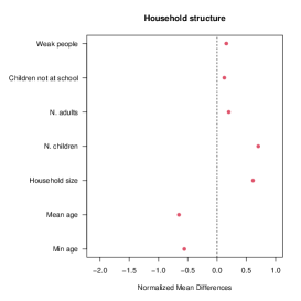
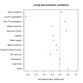
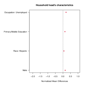
Figure 6. Bolsa Família study: Mixture-model Bayesian analysis. Posterior median of the Normalized mean differences for families in $\mathcal{U}_{s_{0}}$.

Appendix D Simulation Studies

We conduct extensive simulation studies to investigate how our approach works in challenging scenarios. The primary aim of our simulation studies is to shed light on the sources of identification of subpopulation membership. In our Bayesian model-based finite mixture approach to clustering the covariates and the outcome model play a crucial role in classifying units into the three subpopulations, $\mathcal{U}_{s_{0}}$, $\mathcal{U}_{s_{0}}^{-}$, and $\mathcal{U}_{s_{0}}^{+}$. Because units belonging to a subpopulation $\mathcal{U}_{s_{0}}$ should have characteristics such that their probability to fall on either side of the threshold is sufficiently far away from zero and one, $\mathcal{U}_{s_{0}}$ should comprise treated and control units, i.e., units with a realized value of the forcing variable falling below and above the threshold, with similar background characteristics. In a subpopulation $\mathcal{U}_{s_{0}}$, local-SUTVA (Assumption 2) and local unconfoundedness (Assumption 3) hold, and thus, potential outcomes and forcing variable are structurally and statistically independent for units belonging to $\mathcal{U}_{s_{0}}$. For units belonging to either $\mathcal{U}_{s_{0}}^{-}$ or $\mathcal{U}_{s_{0}}^{+}$, local-SUTVA or local unconfoundedness does not hold, implying that potential outcomes depend on the forcing variable.

As an extreme scenario, we consider an RD study where there are no units in $\mathcal{U}_{s_{0}}$, i.e., $\mathcal{U}_{s_{0}}$ is empty. A key concern is whether our procedure is able to recognize that the subpopulation is empty or whether, instead, it wrongly creates a “fake” subpopulation $\mathcal{U}_{s_{0}}$ selecting observations such that the dependency between the outcome and the forcing variable is broken.

Data Generating Processes.

We consider three simulation settings. The first setting focuses on RD studies where there are no units in $\mathcal{U}_{s_{0}}$; the second setting aims to investigate the role of covariates for classifying units into the three subpopulations, $\mathcal{U}_{s_{0}}$, $\mathcal{U}_{s_{0}}^{-}$, and $\mathcal{U}_{s_{0}}^{+}$; and the third setting explores the role of the dependency between the subpopulation membership and the forcing variable. We consider a large sample size $N=10\,000$ to avoid sampling variability issues, and we set $s_{0}=0$.

Data Generating Process: Setting 1.

Under the first setting, data are generated using the following process:

$$\begin{array}[]{ccc}\lx@intercol\hfil\pi_{i}(\mathcal{U}_{s_{0}}^{-})=\pi\qquad\pi_{i}(\mathcal{U}_{s_{0}}^{+})=1-\pi\qquad\pi_{i}(\mathcal{U}_{s_{0}})=0\hfil\lx@intercol\\ \\ S_{i}\mid i\in\mathcal{U}_{s_{0}}^{-}\sim TN\left(\beta_{0}^{-};\sigma^{2}_{-};-\infty,s_{0}\right)&&S_{i}\mid i\in\mathcal{U}_{s_{0}}^{+}\sim TN\left(\beta_{0}^{+};\sigma^{2}_{+};s_{0},\infty\right)\\ \\ Y_{i}(s)\mid i\in\mathcal{U}_{s_{0}}^{-}\sim N\left(\gamma_{0}^{-}+(s-s_{0})\gamma_{1}^{-};\tau^{2}_{-}\right)&&Y_{i}(s)\mid i\in\mathcal{U}_{s_{0}}^{+}\sim N\left(\gamma_{0}^{+}+(s-s_{0})\gamma_{1}^{+};\tau^{2}_{+}\right)\end{array}$$

where $TN(\mu,\sigma^{2},a,b)$ denotes a truncated normal distribution with mean equal to $\mu$ and variance equal to $\sigma^{2}$ before truncation, truncated on the interval $[a,b]$. We set

$$\begin{array}[]{c}\pi=0.75\qquad\beta_{0}^{-}=-2\qquad\sigma^{2}_{-}=1\qquad\beta_{0}^{+}=2.25\qquad\sigma^{2}_{+}=1\qquad\gamma_{0}^{-}=1.75\qquad\gamma_{0}^{+}=0.75\end{array}$$

We consider $3\times 2$ scenarios by varying $\gamma_{1}^{-}$ and $\gamma_{1}^{+}$, which describe the strength of association between the outcome and the forcing variable, and $\tau^{2}_{-}$ and $\tau^{2}_{+}$, the conditional outcome variability given the forcing variable. Specifically, we set

$$\gamma_{1}^{-}=1.5;\gamma_{1}^{+}=1.2\qquad\qquad\gamma_{1}^{-}=1.0;\gamma_{1}^{+}=0.6\qquad\qquad\gamma_{1}^{-}=0.50;\gamma_{1}^{+}=0.30$$

to mimic studies with a strong, medium, and weak association between the outcome and the forcing variable; and

$$\tau^{2}_{-}=\tau^{2}_{+}=0.50^{2}\qquad\qquad\tau^{2}_{-}=\tau^{2}_{+}=0.75^{2}$$

to mimic studies where the outcome variability conditional on the forcing variable is low and high. Table 10 shows the correlation coefficients between the forcing variable and the outcome in the $3\times 2$ scenarios.

Table 10. Simulation setting 1. Correlation coefficients between the forcing variable and the outcome in $\mathcal{U}_{s_{0}}^{-}$ and $\mathcal{U}_{s_{0}}^{-}$, $\rho_{S,Y}^{-}$ and $\rho_{S,Y}^{+}$, in the $3\times 2$ scenarios.

$$\begin{array}[]{c|cc}\lx@intercol\hfil\tau^{2}_{-}=\tau^{2}_{+}=0.50^{2}\hfil\lx@intercol\\ {(\gamma_{1}^{-},\gamma_{1}^{+})}&\rho_{S,Y}^{-}&\rho_{S,Y}^{+}\\ \hline\cr(1.5,1.2)&0.95&0.92\\ (1.0,0.6)&0.89&0.77\\ (0.5,0.3)&0.71&0.51\\ \end{array}\qquad\qquad\begin{array}[]{c|cc}\lx@intercol\hfil\tau^{2}_{-}=\tau^{2}_{+}=0.75^{2}\hfil\lx@intercol\\ {(\gamma_{1}^{-},\gamma_{1}^{+})}&\rho_{S,Y}^{-}&\rho_{S,Y}^{+}\\ \hline\cr(1.5,1.2)&0.89&0.85\\ (1.0,0.6)&0.80&0.63\\ (0.5,0.3)&0.56&0.37\\ \end{array}$$

Data Generating Process: Setting 2.

Under the second setting, data are generated using the following process. We first generate a covariate from a standard Normal distribution and standardize it using the sample mean and the sample variance. Let $X_{i}$ denote the standardized covariate. Then, we generate $G^{\ast}_{i}(-)\sim N\left(\alpha_{0}^{-}+\alpha^{-}_{X}X_{i},1\right)$ and $G^{\ast}_{i}(+)\sim N\left(\alpha_{0}^{+}+\alpha^{+}_{X}X_{i},1\right)$, independently, and we calculate the subpopulation membership probabilities as follows:

$$\pi_{i}(\mathcal{U}_{s_{0}}^{-})=\Pr(G^{\ast}_{i}(-)\leq 0)\qquad\pi_{i}(\mathcal{U}_{s_{0}}^{+})=\Pr(G^{\ast}_{i}(-)>0\,\mathrm{and}\,G^{\ast}_{i}(+)\leq 0)$$

$$\pi_{i}(\mathcal{U}_{s_{0}})=1-\pi_{i}(\mathcal{U}_{s_{0}}^{-})-\pi_{i}(\mathcal{U}_{s_{0}}^{+})\qquad$$

Finally, we generate the forcing variable and the outcome using the following models:

$$\begin{array}[]{ccc}S_{i}\mid i\in\mathcal{U}_{s_{0}}^{-}\sim TN\left(\beta_{0}^{-}+\beta^{-}_{X}X_{i};\sigma^{2}_{-};-\infty,s_{0}\right)&&S_{i}\mid i\in\mathcal{U}_{s_{0}}^{+}\sim TN\left(\beta_{0}^{+}+\beta^{-}_{X}X_{i};\sigma^{2}_{+};s_{0},\infty\right)\\ \vspace{-0.3cm}\hfil\\ \lx@intercol\hfil S_{i}\mid i\in\mathcal{U}_{s_{0}}\sim N\left(\beta_{0}+\beta_{X}X_{i};\sigma^{2}\right)\hfil\lx@intercol\end{array}$$

and

$$\begin{array}[]{ccc}Y_{i}(s)\mid i\in\mathcal{U}_{s_{0}}^{-}\sim N\left(\gamma_{0}^{-}+(s-s_{0})\gamma_{1}^{-}+\gamma^{-}_{X}X_{i};\tau^{2}_{-}\right)&&Y_{i}(s)\mid i\in\mathcal{U}_{s_{0}}^{+}\sim N\left(\gamma_{0}^{+}+(s-s_{0})\gamma_{1}^{+}+\gamma^{+}_{X}X_{i};\tau^{2}_{+}\right)\\ \vspace{-0.3cm}\hfil\\ Y_{i}(0)\mid i\in\mathcal{U}_{s_{0}}\sim N\left(\gamma_{0,z=0}+\gamma_{X,z=0}X_{i};\tau^{2}_{z=0}\right)&&Y_{i}(1)\mid i\in\mathcal{U}_{s_{0}}\sim N\left(\gamma_{0,z=1}+\gamma_{X,z=1}X_{i};\tau^{2}_{z=1}\right)\end{array}$$

We consider eight simulation scenarios, varying: the dependence of the subpopulation membership on the covariate ($\alpha_{X}^{-}$ and $\alpha_{X}^{+}$); the association between the forcing variable and the covariate in each subpopulation, $\mathcal{U}_{s_{0}}^{-}$, $\mathcal{U}_{s_{0}}^{+}$ and $\mathcal{U}_{s_{0}}$ ($\beta_{X}^{-}$, $\beta_{X}^{+}$, and $\beta_{X}$); and the conditional outcome variability given the forcing variable and the covariate in $\mathcal{U}_{s_{0}}^{-}$ and $\mathcal{U}_{s_{0}}^{+}$ ($\tau^{2}_{-}$ and $\tau^{2}_{+}$) and given the covariate in $\mathcal{U}_{s_{0}}$ ($\tau^{2}$). Table 11 shows the true parameter values.

Table 11. Simulation setting 2. True parameter values. Parameters that do not vary across simulation scenarios are shown only for the first scenario

$$\begin{array}[]{c|rr rr rr rr}\hline\cr&\lx@intercol\hfil\hbox{Simulation scenario}\hfil\lx@intercol\\ \hbox{Parameters}&1&2&3&4&5&6&7&8\\ \hline\cr\alpha_{0}^{-}&0.75\\ \alpha_{X}^{-}&0.80&0.80&0.80&0.80&0.40&0.40&0.840&0.40\\ \\ \alpha_{0}^{+}&0.75\\ \alpha_{X}^{+}&-0.40&-0.40&-0.40&-0.40&-0.20&-0.20&-0.20&-0.20\\ \\ \beta_{0}^{-}&-2.00\\ \beta_{X}^{-}&1.50&1.50&0.75&0.75&1.50&1.50&0.75&0.75\\ \sigma^{2}_{-}&1.00&\\ \\ \beta_{0}^{+}&2.25\\ \beta_{X}^{+}&1.25&1.25&0.70&0.70&1.25&1.25&0.70&0.70\\ \sigma^{2}_{+}&1.00\\ \\ \beta_{0}&-1.00\\ \beta_{X}&1.75&1.75&0.80&0.80&1.75&1.75&0.80&0.80\\ \sigma^{2}&1.00\\ \\ \gamma_{0}^{-}&1.75\\ \gamma_{1}^{-}&1.00\\ \gamma_{X}^{-}&0.75\\ \tau^{2}_{-}&0.50^{2}&0.75^{2}&0.50^{2}&0.75^{2}&0.50^{2}&0.75^{2}&0.50^{2}&0.75^{2}\\ \\ \gamma_{0}^{+}&0.75\\ \gamma_{1}^{+}&0.70\\ \gamma_{X}^{+}&0.75\\ \tau^{2}_{+}&0.50^{2}&0.75^{2}&0.50^{2}&0.75^{2}&0.50^{2}&0.75^{2}&0.50^{2}&0.75^{2}\\ \\ \gamma_{0,z=0}&0.50\\ \gamma_{X,z=0}&0.80\\ \tau^{2}_{z=0}&0.50^{2}&0.75^{2}&0.50^{2}&0.75^{2}&0.50^{2}&0.75^{2}&0.50^{2}&0.75^{2}\\ \\ \gamma_{0,z=1}&1.50\\ \gamma_{X,z=1}&0.80\\ \tau^{2}_{z=1}&0.50^{2}&0.75^{2}&0.50^{2}&0.75^{2}&0.50^{2}&0.75^{2}&0.50^{2}&0.75^{2}\\ \hline\cr\end{array}$$

In scenarios 1-4, the dependence of the subpopulation membership on the covariate is relative strong, whereas in scenarios 5-8 it is weaker (see Figure showing the subpopulation membership probabilities as function of the covariate).

Scenarios 1-4		Scenarios 5-8
Strong dependence between		Weak dependence between
subpopulation membership and $X_{i}$		subpopulation membership and $X_{i}$
$\alpha_{X}^{-}=0.8$ and $\alpha_{X}^{+}=-0.4$		$\alpha_{X}^{-}=0.4$ and $\alpha_{X}^{+}=-0.2$

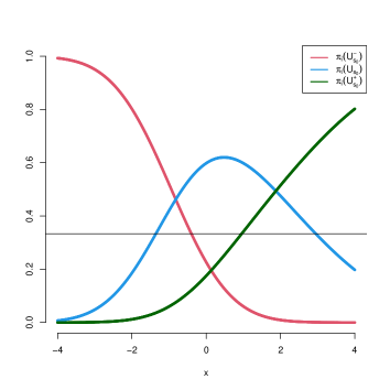
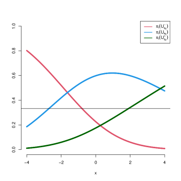
Figure 7. Simulation setting 2. Subpopulation membership probabilities as a function of the covariate

The association between the forcing variable and the covariate in each subpopulation, $\mathcal{U}_{s_{0}}^{-}$, $\mathcal{U}_{s_{0}}^{+}$ and $\mathcal{U}_{s_{0}}$ ($\beta_{X}^{-}$, $\beta_{X}^{+}$, and $\beta_{X}$) is relatively strong in scenarios 1-2 and 5-6, and it is weaker in scenarios 3-4 and 7-8. Table 10 shows the correlation coefficients between the covariate and the forcing variable in the $2\times 2\times 2$ scenarios.

Table 12. Simulation setting 2. Correlation coefficients between the forcing variable and the covariate in $\mathcal{U}_{s_{0}}^{-}$, $\mathcal{U}_{s_{0}}^{+}$ and $\mathcal{U}_{s_{0}}$: $\rho_{X,S}^{-}$, $\rho_{X,S}^{+}$, and $\rho_{X,S}$.

$$\begin{array}[]{lc|ccc}\hbox{Scenario}&{(\beta_{X}^{-},\beta_{X}^{+},\beta_{X})}&\rho_{X,S}^{-}&\rho_{X,S}^{+}&\rho_{X,S}\\ \hline\cr 1,2,5,6&(1.50,1.25,1.75)&0.83&0.78&0.87\\ 3,4,7,8&(0.75,0.70,0.80)&0.60&0.57&0.63\\ \end{array}$$

Finally, a smaller conditional outcome variability is used in scenarios 1, 3, 5, and 7, where we set $\tau^{2}_{-}=\tau^{2}_{+}=\tau^{2,z=0}=\tau^{2,z=1}=0.5^{2}$, and a larger conditional outcome variability is used in scenarios 2,4, 6 and 8 where we set $\tau^{2}_{-}=\tau^{2}_{+}=\tau^{2,z=0}=\tau^{2,z=1}=0.75^{2}$.

Data Generating Process: Setting 3.

Under the third setting, data are generated using the following process:

$$\begin{array}[]{ccc}\lx@intercol\hfil\pi_{i}(\mathcal{U}_{s_{0}}^{-})=0.35\qquad\pi_{i}(\mathcal{U}_{s_{0}}^{+})=0.25\qquad\pi_{i}(\mathcal{U}_{s_{0}})=0.40\hfil\lx@intercol\\ \\ S_{i}\mid i\in\mathcal{U}_{s_{0}}^{-}\sim TN\left(\beta_{0}^{-};\sigma^{2}_{-};-\infty,s_{0}\right)&&S_{i}\mid i\in\mathcal{U}_{s_{0}}^{+}\sim TN\left(\beta_{0}^{+};\sigma^{2}_{+};s_{0},\infty\right)\\ \lx@intercol\hfil S_{i}\mid i\in\mathcal{U}_{s_{0}}\sim N\left(\beta_{0};\sigma^{2}\right)\hfil\lx@intercol\\ \\ Y_{i}(s)\mid i\in\mathcal{U}_{s_{0}}^{-}\sim N\left(\gamma_{0}^{-}+(s-s_{0})\gamma_{1}^{-};\tau^{2}_{-}\right)&&Y_{i}(s)\mid i\in\mathcal{U}_{s_{0}}^{+}\sim N\left(\gamma_{0}^{+}+(s-s_{0})\gamma_{1}^{+};\tau^{2}_{+}\right)\\ Y_{i}(0)\mid i\in\mathcal{U}_{s_{0}}\sim N\left(\gamma_{0,z=0},\tau^{2}_{z=0}\right)&&Y_{i}(01)\mid i\in\mathcal{U}_{s_{0}}\sim N\left(\gamma_{0,z=1},\tau^{2}_{z=1}\right)\\ \end{array}$$

We set $\sigma^{2}_{-}=\sigma^{2}_{+}=\sigma^{2}=1$, $(\gamma_{0}^{-},\gamma_{1}^{-})=(1.75,1.00)$ $(\gamma_{0}^{+},\gamma_{1}^{+})=(0.75,0.60)$, $\gamma_{0,z=0}=0.5$ and $\gamma_{0,z=1}=1.5$, and we vary $\beta_{0}^{-}$, $\beta_{0}^{+}$, and $\beta_{0}$, which describe the strength of association between the forcing variable and subpopulation membership, and outcome variances, $\tau^{2}_{-}$, $\tau^{2}_{+}$ and $\tau^{2}_{z=0}$ and $\tau^{2}_{z=1}$. Specifically, we consider $2\times 2$ scenarios by setting

$$\beta_{0}^{-}=-2.00;\beta_{0}^{+}=2.25;\beta_{0}=-1.00\qquad\hbox{ and }\qquad\beta_{0}^{-}=-0.50;\beta_{0}^{+}=0.75;\beta_{0}=-0.25$$

and

$$\tau^{2}_{-}=\tau^{2}_{+}=\tau^{2}_{z=0}=\tau^{2}_{z=1}=0.50^{2}\qquad\hbox{ and }\qquad\tau^{2}_{-}=\tau^{2}_{+}=\tau^{2}_{z=0}=\tau^{2}_{z=1}=0.75^{2}$$

Figure 8 shows the conditional probabilities of belonging to each membership given the forcing variable, which we derive using the Bayes Theorem as follows:

$$\pi_{i}(\mathcal{U}_{s_{0}}^{-}\mid S_{i}=s) = \dfrac{\pi_{i}(\mathcal{U}_{s_{0}}^{-})f_{S\mid\mathcal{U}_{s_{0}}^{-}}(s)}{\pi_{i}(\mathcal{U}_{s_{0}}^{-})f_{S\mid\mathcal{U}_{s_{0}}^{-}}(s)+\pi_{i}(\mathcal{U}_{s_{0}}^{+})f_{S\mid\mathcal{U}_{s_{0}}^{+}}(s)+\pi_{i}(\mathcal{U}_{s_{0}})f_{S\mid\mathcal{U}_{s_{0}}}(s)}$$

$$\pi_{i}(\mathcal{U}_{s_{0}}^{+}\mid S_{i}=s) = \dfrac{\pi_{i}(\mathcal{U}_{s_{0}}^{+})f_{S\mid\mathcal{U}_{s_{0}}^{+}}(s)}{\pi_{i}(\mathcal{U}_{s_{0}}^{-})f_{S\mid\mathcal{U}_{s_{0}}^{-}}(s)+\pi_{i}(\mathcal{U}_{s_{0}}^{+})f_{S\mid\mathcal{U}_{s_{0}}^{+}}(s)+\pi_{i}(\mathcal{U}_{s_{0}})f_{S\mid\mathcal{U}_{s_{0}}}(s)}$$

$$\pi_{i}(\mathcal{U}_{s_{0}}\mid S_{i}=s) = \dfrac{\pi(\mathcal{U}_{s_{0}})f_{S\mid\mathcal{U}_{s_{0}}}(s)}{\pi_{i}(\mathcal{U}_{s_{0}}^{-})f_{S\mid\mathcal{U}_{s_{0}}^{-}}(s)+\pi_{i}(\mathcal{U}_{s_{0}}^{+})f_{S\mid\mathcal{U}_{s_{0}}^{+}}(s)+\pi_{i}(\mathcal{U}_{s_{0}})f_{S\mid\mathcal{U}_{s_{0}}}(s)}$$

with $f_{S\mid\mathcal{U}_{s_{0}}^{-}}(s)=0$ for $s>s_{0}$ and $f_{S\mid\mathcal{U}_{s_{0}}^{+}}(s)=0$ for $s\leq s_{0}$.

Scenarios 1 and 3		Scenarios 2 and 4
Strong dependence between		Weak dependence between
subpopulation membership and $S_{i}$		subpopulation membership and $S_{i}$
$\beta_{0}^{-}=-2.00;\beta_{0}^{+}=2.25;\beta_{0}=-1.00$		$\beta_{0}^{-}=-0.50;\beta_{0}^{+}=0.75;\beta_{0}=-0.25$

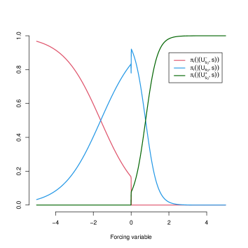
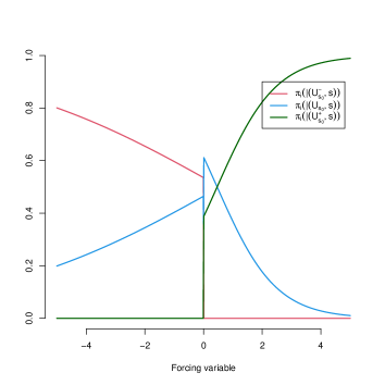
Figure 8. Simulation setting 3. Subpopulation membership probabilities as a function of the forcing variable

Simulation Results.

For each scenario in each simulation setting, we apply our Bayesian model-based mixture approach to clustering to $50$ simulated datasets of size $N=10\,000$. We evaluate the performance of our procedure using the average of the posterior means over the 50 datasets, the bias, the mean squared error (MSE), and the coverage of the 95% and 99% highest density interval of each causal estimand of interest.

Simulation Results: Setting 1.

Simulation setting 1 focuses on studies where there is no unit in $\mathcal{U}_{s_{0}}$ aiming to investigate if our procedure successfully detects that the subpopulation $\mathcal{U}_{s_{0}}$ is empty rather than create a “fake” subpopulation $\mathcal{U}_{s_{0}}$ by selecting observations such that the dependence between the outcome and the forcing variable is broken. Table 13 shows that our Bayesian model-based mixture approach provides extremely small posterior means for the proportion of units in $\mathcal{U}_{s_{0}}$ with a very high precision (small bias, small MSE, and high coverage) under each scenario, successfully suggesting that the subpopulation $\mathcal{U}_{s_{0}}$ is empty. As we expected, the stronger the association between the forcing variable and the outcome, the stronger the evidence that $\mathcal{U}_{s_{0}}$ is empty is.

In this setting, looking at causal effects for units in the subpopulation $\mathcal{U}_{s_{0}}$ does not make sense. It might be sensible to look at causal effects at the threshold, such as the average causal effect at $s_{0}$:

$$ACE_{s_{0}}=\lim\limits_{s\uparrow s_{0}}\mathbb{E}[Y_{i}(s)\mid S_{i}=s]-\lim\limits_{s\downarrow s_{0}}\mathbb{E}[Y_{i}(s)\mid S_{i}=s]$$

Under our data generating process, $\tau_{s_{0}}=\gamma_{0}^{-}-\gamma_{0}^{+}=1.75-0.75=1$. Table 13 shows the results, which suggest that our Bayesian model-based mixture approach leads to a posterior distribution of the average causal effect at $s_{0}$ centered around the true value with good frequentistic properties.

Table 13. Simulation setting 1: Simulation results on $\pi(\mathcal{U}_{s_{0}})$. Average of the posterior means, bias, MSE, and 95% and 99% coverage for the proportion of units in $\mathcal{U}_{s_{0}}$. True value: $\pi(\mathcal{U}_{s_{0}})=0$.

$$\begin{array}[]{ll ccccc}\lx@intercol\hfil\hbox{Conditional outcome variance given the forcing variable: }\tau^{2}_{-}=\tau^{2}_{+}=0.50^{2}\hfil\lx@intercol\\ \hline\cr&&\hbox{Average of the}&&&\lx@intercol\hfil\hbox{Coverage}\hfil\lx@intercol\\ \cline{6-7}\cr\lx@intercol\hbox{$S-Y$ association}\hfil\lx@intercol&\hbox{Posterior Means}&\hbox{Bias}&\hbox{MSE}&\hbox{95\% HDI }&\hbox{99\% HDI}\\ \hline\cr\hbox{Strong: }&\gamma_{1}^{-}=1.5;\gamma_{1}^{+}=1.2&0.000006&0.000006&0.0000&1.00&1.00\\ \vspace{-0.35cm}\\ \hbox{Medium: }&\gamma_{1}^{-}=1.0;\gamma_{1}^{+}=0.6&0.000035&0.000035&1.0/10^{7}&1.00&1.00\\ \vspace{-0.35cm}\\ \hbox{Weak: }&\gamma_{1}^{-}=0.5;\gamma_{1}^{+}=0.3&0.000346&0.000346&2.2/10^{6}&0.98&0.98\\ \hline\cr\end{array}$$

$$\begin{array}[]{ll ccccc}\lx@intercol\hfil\hbox{Conditional outcome variance given the forcing variable: }\tau^{2}_{-}=\tau^{2}_{+}=0.75^{2}\hfil\lx@intercol\\ \hline\cr&&\hbox{Average of the}&&&\lx@intercol\hfil\hbox{Coverage}\hfil\lx@intercol\\ \cline{6-7}\cr\lx@intercol\hbox{$S-Y$ association}\hfil\lx@intercol&\hbox{Posterior Means}&\hbox{Bias}&\hbox{MSE}&\hbox{95\% HDI }&\hbox{99\% HDI}\\ \hline\cr\hbox{Strong: }&\gamma_{1}^{-}=1.5;\gamma_{1}^{+}=1.2&0.000070&0.000070&1.0/10^{7}&0.98&0.98\\ \vspace{-0.35cm}\\ \hbox{Medium: }&\gamma_{1}^{-}=1.0;\gamma_{1}^{+}=0.6&0.000077&0.000077&3.0/10^{7}&0.98&0.98\\ \vspace{-0.35cm}\\ \hbox{Weak: }&\gamma_{1}^{-}=0.5;\gamma_{1}^{+}=0.3&0.000003&0.000003&0.0000&1.00&1.00\\ \hline\cr\end{array}$$

Table 14. Simulation setting 1: Simulation results on $ACE_{s_{0}}$. Average of the posterior means, bias, MSE, and 95% and 99% coverage for $\tau_{s_{0}}$. True value: $ACE_{s_{0}}=1$.

$$\begin{array}[]{ll ccccc}\lx@intercol\hfil\hbox{Conditional outcome variance given the forcing variable: }\tau^{2}_{-}=\tau^{2}_{+}=0.50^{2}\hfil\lx@intercol\\ \hline\cr&&\hbox{Average of the}&&&\lx@intercol\hfil\hbox{Coverage}\hfil\lx@intercol\\ \cline{6-7}\cr\lx@intercol\hbox{$S-Y$ association}\hfil\lx@intercol&\hbox{Posterior Means}&\hbox{Bias}&\hbox{MSE}&\hbox{95\% HDI }&\hbox{99\% HDI}\\ \hline\cr\hbox{Strong: }&\gamma_{1}^{-}=1.5;\gamma_{1}^{+}=1.2&0.9940&-0.0060&0.0007&0.96&0.98\\ \vspace{-0.35cm}\\ \hbox{Medium: }&\gamma_{1}^{-}=1.0;\gamma_{1}^{+}=0.6&0.9942&-0.0058&0.0008&0.96&0.98\\ \vspace{-0.35cm}\\ \hbox{Weak: }&\gamma_{1}^{-}=0.5;\gamma_{1}^{+}=0.3&0.9939&-0.0061&0.0008&0.96&1.00\\ \hline\cr\end{array}$$

$$\begin{array}[]{ll ccccc}\lx@intercol\hfil\hbox{Conditional outcome variance given the forcing variable: }\tau^{2}_{-}=\tau^{2}_{+}=0.75^{2}\hfil\lx@intercol\\ \hline\cr&&\hbox{Average of the}&&&\lx@intercol\hfil\hbox{Coverage}\hfil\lx@intercol\\ \cline{6-7}\cr\lx@intercol\hbox{$S-Y$ association}\hfil\lx@intercol&\hbox{Posterior Means}&\hbox{Bias}&\hbox{MSE}&\hbox{95\% HDI }&\hbox{99\% HDI}\\ \hline\cr\hbox{Strong: }&\gamma_{1}^{-}=1.5;\gamma_{1}^{+}=1.2&0.9911&-0.0089&0.0017&0.96&0.96\\ \vspace{-0.35cm}\\ \hbox{Medium: }&\gamma_{1}^{-}=1.0;\gamma_{1}^{+}=0.6&0.9900&-0.0100&0.0018&0.96&0.98\\ \vspace{-0.35cm}\\ \hbox{Weak: }&\gamma_{1}^{-}=0.5;\gamma_{1}^{+}=0.3&0.9905&-0.0095&0.0018&0.96&1.00\\ \hline\cr\end{array}$$

Simulation Results: Setting 2.

In setting 2 we focus on the proportion of units in $\mathcal{U}_{s_{0}}$:

$$\pi(\mathcal{U}_{s_{0}})=\dfrac{N_{\mathcal{U}_{s_{0}}}}{N}$$

where $N_{\mathcal{U}_{s_{0}}}$ is the number of units belonging to $\mathcal{U}_{s_{0}}$ and the average causal effect for units in $\mathcal{U}_{s_{0}}$:

$$ACE_{\mathcal{U}_{s_{0}}}=\dfrac{1}{N_{\mathcal{U}_{s_{0}}}}\sum_{i\in\mathcal{U}_{s_{0}}}Y_{i}(1)-\dfrac{1}{N_{\mathcal{U}_{s_{0}}}}\sum_{i\in\mathcal{U}_{s_{0}}}Y_{i}(0)$$

Results shown in Table 15 highlight the importance of observing covariates that are predictive of the subpopulation membership and the forcing variable. In particular, our simulation study reveals that the association between the covariate and forcing variable play a special role. The stronger the association between the covariate and forcing variable, the better the performance of the Bayesian model-based approach to clustering is.

Table 15. Simulation setting 2: Simulation results. Average of the posterior means, bias, MSE, and 95% and 99% coverage for $\pi(\mathcal{U}_{s_{0}})$ and $ACE_{\mathcal{U}_{s_{0}}}$.

$$\begin{array}[]{ccc rcrccc}\lx@intercol\hfil\hbox{Conditional outcome variance given the forcing variable: }\tau^{2}_{-}=\tau^{2}_{+}=\tau^{2}=0.50^{2}\hfil\lx@intercol\\ \lx@intercol\hfil\hbox{Dependence of the subpopulation membership on the covariate: }\alpha_{X}^{-}=0.8\hbox{ and }\alpha_{X}^{+}=-0.40\hfil\lx@intercol\\ \vspace{-0.35cm}\hfil\\ \hline\cr\lx@intercol\hbox{$S-X$ association}\hfil\lx@intercol&&\hbox{Average of the}&&&\lx@intercol\hfil\hbox{Coverage}\hfil\lx@intercol\\ \cline{8-9}\cr\beta_{X}^{-}&\beta_{X}^{+}&\beta_{X}&\hbox{True value}&\hbox{Posterior Means}&\hbox{Bias}&\hbox{MSE}&\hbox{95\% HDI }&\hbox{99\% HDI}\\ \hline\cr 1.50&1.25&1.75&\pi_{i}(\mathcal{U}_{s_{0}})=0.5211&0.5232&0.0020&0.0000&0.98&1.00\\ &&&ACE_{\mathcal{U}_{s_{0}}}=1.0003&0.9917&-0.0085&0.0007&0.86&0.94\\ \vspace{-0.25cm}\hfil\\ 0.75&0.70&0.80&\pi_{i}(\mathcal{U}_{s_{0}})=0.5221&0.5096&-0.0125&0.0039&0.64&0.84\\ &&&ACE_{\mathcal{U}_{s_{0}}}=1.0013&1.0449&0.0436&0.0580&0.78&0.88\\ \hline\cr\end{array}$$

$$\begin{array}[]{ccc rcrccc}\lx@intercol\hfil\hbox{Conditional outcome variance given the forcing variable: }\tau^{2}_{-}=\tau^{2}_{+}=\tau^{2}=0.50^{2}\hfil\lx@intercol\\ \lx@intercol\hfil\hbox{Dependence of the subpopulation membership on the covariate: }\alpha_{X}^{-}=0.4\hbox{ and }\alpha_{X}^{+}=-0.20\hfil\lx@intercol\\ \vspace{-0.35cm}\hfil\\ \hline\cr\lx@intercol\hbox{$S-X$ association}\hfil\lx@intercol&&\hbox{Average of the}&&&\lx@intercol\hfil\hbox{Coverage}\hfil\lx@intercol\\ \cline{8-9}\cr\beta_{X}^{-}&\beta_{X}^{+}&\beta_{X}&\hbox{True value}&\hbox{Posterior Means}&\hbox{Bias}&\hbox{MSE}&\hbox{95\% HDI }&\hbox{99\% HDI}\\ \hline\cr 1.50&1.25&1.75&\pi_{i}(\mathcal{U}_{s_{0}})=0.5749&0.5777&0.0028&0.0000&0.82&0.94\\ &&&ACE_{\mathcal{U}_{s_{0}}}=1.0000&1.0018&0.0019&0.0006&0.88&0.94\\ \vspace{-0.25cm}\hfil\\ 0.75&0.70&0.80&\pi_{i}(\mathcal{U}_{s_{0}})=0.5746&0.5753&0.0008&0.0029&0.60&0.82\\ &&&ACE_{\mathcal{U}_{s_{0}}}=1.0002&1.0074&0.0072&0.0192&0.88&0.94\\ \hline\cr\end{array}$$

$$\begin{array}[]{ccc rcrccc}\lx@intercol\hfil\hbox{Conditional outcome variance given the forcing variable: }\tau^{2}_{-}=\tau^{2}_{+}=\tau^{2}=0.75^{2}\hfil\lx@intercol\\ \lx@intercol\hfil\hbox{Dependence of the subpopulation membership on the covariate: }\alpha_{X}^{-}=0.8\hbox{ and }\alpha_{X}^{+}=-0.40\hfil\lx@intercol\\ \vspace{-0.35cm}\hfil\\ \hline\cr\lx@intercol\hbox{$S-X$ association}\hfil\lx@intercol&&\hbox{Average of the}&&&\lx@intercol\hfil\hbox{Coverage}\hfil\lx@intercol\\ \cline{8-9}\cr\beta_{X}^{-}&\beta_{X}^{+}&\beta_{X}&\hbox{True value}&\hbox{Posterior Means}&\hbox{Bias}&\hbox{MSE}&\hbox{95\% HDI }&\hbox{99\% HDI}\\ \hline\cr 1.50&1.25&1.75&\pi_{i}(\mathcal{U}_{s_{0}})=0.5214&0.5263&0.0049&0.0000&0.82&0.94\\ \\ &&&ACE_{\mathcal{U}_{s_{0}}}=1.0009&0.9865&-0.0144&0.0016&0.90&0.96\\ \vspace{-0.25cm}\hfil\\ 0.75&0.70&0.80&\pi_{i}(\mathcal{U}_{s_{0}})=0.5224&0.5227&0.0004&0.0022&0.64&0.86\\ &&&ACE_{\mathcal{U}_{s_{0}}}=1.0019&1.0003&-0.0016&0.0331&0.82&0.94\\ \hline\cr\end{array}$$

$$\begin{array}[]{ccc rcrccc}\lx@intercol\hfil\hbox{Conditional outcome variance given the forcing variable: }\tau^{2}_{-}=\tau^{2}_{+}=\tau^{2}=0.75^{2}\hfil\lx@intercol\\ \lx@intercol\hfil\hbox{Dependence of the subpopulation membership on the covariate: }\alpha_{X}^{-}=0.4\hbox{ and }\alpha_{X}^{+}=-0.20\hfil\lx@intercol\\ \vspace{-0.35cm}\hfil\\ \hline\cr\lx@intercol\hbox{$S-X$ association}\hfil\lx@intercol&&\hbox{Average of the}&&&\lx@intercol\hfil\hbox{Coverage}\hfil\lx@intercol\\ \cline{8-9}\cr\beta_{X}^{-}&\beta_{X}^{+}&\beta_{X}&\hbox{True value}&\hbox{Posterior Means}&\hbox{Bias}&\hbox{MSE}&\hbox{95\% HDI }&\hbox{99\% HDI}\\ \hline\cr 1.50&1.25&1.75&\pi_{i}(\mathcal{U}_{s_{0}})=0.5745&0.5798&0.0053&0.0001&0.78&0.88\\ &&&ACE_{\mathcal{U}_{s_{0}}}=1.0004&0.9988&-0.0015&0.0013&0.94&0.94\\ \\ \vspace{-0.25cm}\hfil\\ 0.75&0.70&0.80&\pi_{i}(\mathcal{U}_{s_{0}})=0.5748&0.5768&0.0020&0.0051&0.34&0.54\\ &&&ACE_{\mathcal{U}_{s_{0}}}=1.0018&1.0011&-0.0008&0.0211&0.78&0.90\\ \hline\cr\end{array}$$

Simulation Results: Setting 3.

In setting 3 we again focus on the proportion of units in $\mathcal{U}_{s_{0}}$, $\pi(\mathcal{U}_{s_{0}})$ and the average causal effect for units in $\mathcal{U}_{s_{0}}$, $ACE_{\mathcal{U}_{s_{0}}}$. Table 16 shows the results, which suggest that the Bayesian model-mixture approach to clustering we propose leads to more accurate and more efficient estimates of the causal estimands (that is, estimates with smaller bias, smaller MSE, and higher coverage) in studies where the dependence of subpopulation membership on the forcing variable is stronger.

Table 16. Simulation setting 3: Simulation results. Average of the posterior means, bias, MSE, and 95% and 99% coverage for $\pi(\mathcal{U}_{s_{0}})$ and $ACE_{\mathcal{U}_{s_{0}}}$.

$$\begin{array}[]{ccc rcrccc}\lx@intercol\hfil\hbox{Conditional outcome variance given the forcing variable: }\tau^{2}_{-}=\tau^{2}_{+}=\tau^{2}=0.50^{2}\hfil\lx@intercol\\ \vspace{-0.35cm}\hfil\\ \hline\cr&&&&\hbox{Average of the}&&&\lx@intercol\hfil\hbox{Coverage}\hfil\lx@intercol\\ \cline{8-9}\cr\beta_{0}^{-}&\beta_{0}^{+}&\beta_{0}&\hbox{True value}&\hbox{Posterior Means}&\hbox{Bias}&\hbox{MSE}&\hbox{95\% HDI }&\hbox{99\% HDI}\\ \hline\cr-2.00&2.25&-1.00&\pi(\mathcal{U}_{s_{0}})=0.4002&0.3999&-0.0002&0.0001&0.94&1.00\\ &&&ACE_{\mathcal{U}_{s_{0}}}=1.0012&1.0014&0.0003&0.0007&0.96&1.00\\ \vspace{-0.25cm}\hfil\\ -0.50&0.75&-0.25&\pi(\mathcal{U}_{s_{0}})=0.4006&0.3979&-0.0026&0.0003&0.94&0.98\\ &&&ACE_{\mathcal{U}_{s_{0}}}=1.0010&1.0036&0.0026&0.0014&0.94&0.96\\ \vspace{-0.25cm}\hfil\\ \hline\cr\end{array}$$

$$\begin{array}[]{ccc rcrccc}\lx@intercol\hfil\hbox{Conditional outcome variance given the forcing variable: }\tau^{2}_{-}=\tau^{2}_{+}=\tau^{2}=0.75^{2}\hfil\lx@intercol\\ \vspace{-0.35cm}\hfil\\ \hline\cr&&&&\hbox{Average of the}&&&\lx@intercol\hfil\hbox{Coverage}\hfil\lx@intercol\\ \cline{8-9}\cr\beta_{0}^{-}&\beta_{0}^{+}&\beta_{0}&\hbox{True value}&\hbox{Posterior Means}&\hbox{Bias}&\hbox{MSE}&\hbox{95\% HDI }&\hbox{99\% HDI}\\ \hline\cr-2.00&2.25&-1.00&\pi(\mathcal{U}_{s_{0}})=0.3999&0.3979&-0.0020&0.0002&0.88&0.98\\ &&&ACE_{\mathcal{U}_{s_{0}}}=1.0020&1.0025&0.0004&0.0018&0.96&0.98\\ \vspace{-0.25cm}\hfil\\ -0.50&0.75&-0.25&\pi(\mathcal{U}_{s_{0}})=0.4002&0.3957&-0.0045&0.0009&0.90&1.00\\ &&&ACE_{\mathcal{U}_{s_{0}}}=1.0008&1.0003&-0.0005&0.0068&0.90&0.98\\ \hline\cr\end{array}$$

Appendix E Covariate Balance in Specific MSE-optimal Sub-populations

Tables 17-20 show the posterior median of the sample averages and standard deviations by eligibility status, and the three measures of balancing–the normalized differences; the log of the ratio of the sample standard deviations; and the Mahalanobis distance between the means–within four MSE-optimal subpopulations. Specifically, the four MSE-optimal subpopulations have been selected the MSE-optimal bandwidth approach based on the uniform and the triangular kernel functions and the local-polynomial estimators of order $p=1$ and $p=2$. Figure 9 shows graphically the normalized differences within the four MSE-optimal subpopulations.

Table 17. Bolsa Família study: Covariate balance within the sub-population $\mathcal{U}_{s_{0}}=\{i:43.5\leq S_{i}\leq 163.9\}$, selected using the MSE-optimal bandwidth approach based on the uniform kernel function and the local-polynomial estimator of order $p=1$

$$\begin{array}[]{lrrrrrr}\hline\cr\vspace{-0.35cm}\\ &\lx@intercol\hfil\hbox{Ineligible}\hfil\lx@intercol&\lx@intercol\hfil\hbox{Eligible}\hfil\lx@intercol\\ N_{\mathcal{U}_{s_{0}}}=69\,796&\lx@intercol\hfil(4\,852)\hfil\lx@intercol&\lx@intercol\hfil(64\,944)\hfil\lx@intercol&\hbox{Norm.}&\\ \vspace{-0.4cm}\\ \hbox{Covariate}&\hbox{Mean}&\hbox{SD}&\hbox{Mean}&\hbox{SD}&\hbox{Diff.}&\log(s_{1}/s_{0})\\ \vspace{-0.35cm}\\ \hline\cr\vspace{-0.35cm}\\ \lx@intercol\hbox{{Household structure}}\hfil\lx@intercol\\ \vspace{-0.4cm}\\ \hbox{Min age}&14.68&15.74&13.15&15.56&-0.10&-0.01\\ \hbox{Mean age}&28.84&12.84&24.56&12.10&-0.34&-0.06\\ \hbox{Household size}&2.80&1.05&2.81&1.26&0.01&0.19\\ \hbox{N. Children}&0.90&0.76&1.12&0.97&0.26&0.25\\ \hbox{N. Adults}&1.71&0.78&1.63&0.76&-0.11&-0.03\\ \hbox{Children not at school}&0.02&0.14&0.03&0.17&0.07&0.20\\ \hbox{Presence of weak people}&0.18&0.38&0.20&0.40&0.06&0.04\\ \vspace{-0.3cm}\\ \lx@intercol\hbox{{Living and economic conditions}}\hfil\lx@intercol\\ \vspace{-0.4cm}\\ \hbox{Rural}&0.22&0.41&0.31&0.46&0.22&0.12\\ \hbox{Apartment}&0.95&0.21&0.95&0.22&-0.02&0.04\\ \hbox{Home ownership: Homeowner}&0.64&0.48&0.58&0.49&-0.13&0.03\\ \hbox{No rooms pc}&1.82&1.10&1.77&1.14&-0.05&0.04\\ \hbox{House of bricks/row dirt }&0.95&0.22&0.92&0.26&-0.10&0.18\\ \hbox{Water treatment}&0.85&0.35&0.83&0.37&-0.06&0.05\\ \hbox{Water supply}&0.76&0.43&0.69&0.46&-0.15&0.08\\ \hbox{Lighting}&0.91&0.29&0.84&0.36&-0.19&0.21\\ \hbox{Bathroom fixture}&0.47&0.50&0.55&0.50&0.17&0.00\\ \hbox{Waste treatment}&0.81&0.39&0.72&0.45&-0.21&0.13\\ \hbox{Zero PC expenditure}&0.15&0.36&0.17&0.38&0.05&0.04\\ \hbox{Log PC expenditure}&3.83&1.76&3.36&1.65&-0.28&-0.06\\ \hbox{Other programs}&0.05&0.22&0.05&0.21&-0.01&-0.02\\ \vspace{-0.3cm}\\ \lx@intercol\hbox{{Household head's characteristics}}\hfil\lx@intercol\\ \vspace{-0.4cm}\\ \hbox{Male}&0.85&0.35&0.85&0.36&-0.02&0.02\\ \hbox{Race: Hispanic}&0.86&0.34&0.88&0.33&0.04&-0.05\\ \hbox{Primary/Middle Education}&0.39&0.49&0.42&0.49&0.08&0.01\\ \hbox{Occupation: Unemployed}&0.43&0.50&0.50&0.50&0.13&0.01\\ \vspace{-0.2cm}\\ \hbox{Multivariate measure}&&&&&0.91\\ \vspace{-0.35cm}\\ \hline\cr\end{array}$$

Table 18. Bolsa Família study: Weighted covariate balance within the sub-population $\mathcal{U}_{s_{0}}=\{i:39.0\leq S_{i}\leq 174.5\}$, selected using the MSE-optimal bandwidth approach based on the triangular kernel function and the local-polynomial estimator of order $p=1$ (Weights based on the triangular Kernel)

$$\begin{array}[]{lrrrrrr}\hline\cr\vspace{-0.35cm}\\ &\lx@intercol\hfil\hbox{Ineligible}\hfil\lx@intercol&\lx@intercol\hfil\hbox{Eligible}\hfil\lx@intercol\\ N_{\mathcal{U}_{s_{0}}}=83\,326&\lx@intercol\hfil(=5\,159)\hfil\lx@intercol&\lx@intercol\hfil(78\,167)\hfil\lx@intercol&\hbox{Norm.}&\\ \vspace{-0.4cm}\\ \hbox{Covariate}&\hbox{Mean}&\hbox{SD}&\hbox{Mean}&\hbox{SD}&\hbox{Diff.}&\log(s_{1}/s_{0})\\ \vspace{-0.35cm}\\ \hline\cr\vspace{-0.35cm}\\ \lx@intercol\hbox{{Household structure}}\hfil\lx@intercol\\ \vspace{-0.4cm}\\ \hbox{Min age}&13.25&14.87&12.96&15.17&-0.02&0.02\\ \hbox{Mean age}&28.02&12.52&25.19&11.90&-0.23&-0.05\\ \hbox{Household size}&2.86&0.99&2.90&1.26&0.03&0.24\\ \hbox{N. Children}&0.95&0.75&1.13&0.95&0.21&0.24\\ \hbox{N. Adults}&1.73&0.77&1.68&0.78&-0.07&0.01\\ \hbox{Children not at school}&0.02&0.15&0.03&0.18&0.07&0.19\\ \hbox{Presence of weak people}&0.19&0.39&0.20&0.40&0.04&0.03\\ \vspace{-0.3cm}\\ \lx@intercol\hbox{{Living and economic conditions}}\hfil\lx@intercol\\ \vspace{-0.4cm}\\ \hbox{Rural}&0.21&0.41&0.28&0.45&0.16&0.10\\ \hbox{Apartment}&0.95&0.22&0.95&0.22&-0.02&0.03\\ \hbox{Home ownership: Homeowner}&0.64&0.48&0.59&0.49&-0.09&0.02\\ \hbox{No rooms pc}&1.73&1.01&1.75&1.14&0.02&0.13\\ \hbox{House of bricks/row dirt }&0.95&0.22&0.93&0.25&-0.07&0.13\\ \hbox{Water treatment}&0.85&0.35&0.84&0.37&-0.04&0.03\\ \hbox{Water supply}&0.76&0.43&0.72&0.45&-0.10&0.06\\ \hbox{Lighting}&0.91&0.29&0.87&0.34&-0.14&0.17\\ \hbox{Bathroom fixture}&0.46&0.50&0.53&0.50&0.13&0.00\\ \hbox{Waste treatment}&0.82&0.39&0.75&0.43&-0.16&0.11\\ \hbox{Zero PC expenditure}&0.15&0.36&0.17&0.37&0.04&0.04\\ \hbox{Log PC expenditure}&3.82&1.76&3.48&1.70&-0.19&-0.03\\ \hbox{Other programs}&0.05&0.22&0.05&0.21&-0.02&-0.03\\ \vspace{-0.3cm}\\ \lx@intercol\hbox{{Household head's characteristics}}\hfil\lx@intercol\\ \vspace{-0.4cm}\\ \hbox{Male}&0.86&0.34&0.85&0.36&-0.05&0.05\\ \hbox{Race: Hispanic}&0.87&0.34&0.88&0.33&0.03&-0.03\\ \hbox{Primary/Middle Education}&0.37&0.48&0.41&0.49&0.07&0.02\\ \hbox{Occupation: Unemployed}&0.45&0.50&0.49&0.50&0.07&0.00\\ \vspace{-0.2cm}\\ \hbox{Multivariate measure}&&&&&0.67\\ \vspace{-0.3cm}\\ \hline\cr\end{array}$$

Table 19. Bolsa Família study: Covariate balance within the sub-population $\mathcal{U}_{s_{0}}=\{i:0.0\leq S_{i}\leq 166.0\}$, selected using the MSE-optimal bandwidth approach based on the uniform kernel function and the local-polynomial estimator of order $p=2$

$$\begin{array}[]{lrrrrrr}\hline\cr\vspace{-0.35cm}\\ &\lx@intercol\hfil\hbox{Ineligible}\hfil\lx@intercol&\lx@intercol\hfil\hbox{Eligible}\hfil\lx@intercol\\ N_{\mathcal{U}_{s_{0}}}=143\,102&\lx@intercol\hfil(4\,882)\hfil\lx@intercol&\lx@intercol\hfil(138\,220)\hfil\lx@intercol&\hbox{Norm.}&\\ \vspace{-0.4cm}\\ \hbox{Covariate}&\hbox{Mean}&\hbox{SD}&\hbox{Mean}&\hbox{SD}&\hbox{Diff.}&\log(s_{1}/s_{0})\\ \vspace{-0.35cm}\\ \hline\cr\vspace{-0.35cm}\\ \lx@intercol\hbox{{Household structure}}\hfil\lx@intercol\\ \vspace{-0.4cm}\\ \hbox{Min age}&14.67&15.72&10.32&13.85&-0.29&-0.13\\ \hbox{Mean age}&28.84&12.82&21.89&11.28&-0.58&-0.13\\ \hbox{Household size}&2.81&1.05&3.02&1.32&0.18&0.23\\ \hbox{N. Children}&0.90&0.76&1.38&1.11&0.51&0.38\\ \hbox{N. Adults}&1.72&0.78&1.60&0.74&-0.15&-0.07\\ \hbox{Children not at school}&0.02&0.14&0.04&0.20&0.11&0.32\\ \hbox{Presence of weak people}&0.18&0.38&0.23&0.42&0.11&0.08\\ \vspace{-0.3cm}\\ \lx@intercol\hbox{{Living and economic conditions}}\hfil\lx@intercol\\ \vspace{-0.4cm}\\ \hbox{Rural}&0.22&0.41&0.40&0.49&0.42&0.18\\ \hbox{Apartment}&0.95&0.21&0.95&0.22&-0.01&0.03\\ \hbox{Home ownership: Homeowner}&0.64&0.48&0.58&0.49&-0.12&0.03\\ \hbox{No rooms pc}&1.82&1.10&1.57&1.02&-0.23&-0.07\\ \hbox{House of bricks/row dirt }&0.95&0.22&0.91&0.29&-0.15&0.26\\ \hbox{Water treatment}&0.85&0.35&0.78&0.41&-0.18&0.15\\ \hbox{Water supply}&0.76&0.43&0.63&0.48&-0.29&0.12\\ \hbox{Lighting}&0.91&0.29&0.79&0.41&-0.34&0.34\\ \hbox{Bathroom fixture}&0.47&0.50&0.62&0.49&0.31&-0.03\\ \hbox{Waste treatment}&0.81&0.39&0.63&0.48&-0.42&0.21\\ \hbox{Zero PC expenditure}&0.15&0.36&0.22&0.41&0.17&0.14\\ \hbox{Log PC expenditure}&3.83&1.75&2.89&1.67&-0.55&-0.05\\ \hbox{Other programs}&0.05&0.22&0.06&0.23&0.04&0.07\\ \vspace{-0.3cm}\\ \lx@intercol\hbox{{Household head's characteristics}}\hfil\lx@intercol\\ \vspace{-0.4cm}\\ \hbox{Male}&0.85&0.35&0.87&0.34&0.03&-0.03\\ \hbox{Race: Hispanic}&0.86&0.34&0.88&0.32&0.06&-0.07\\ \hbox{Primary/Middle Education}&0.39&0.49&0.47&0.50&0.17&0.02\\ \hbox{Occupation: Unemployed}&0.43&0.50&0.49&0.50&0.13&0.01\\ \vspace{-0.2cm}\\ \hbox{Multivariate measure}&&&&&1.33\\ \vspace{-0.3cm}\\ \hline\cr\end{array}$$

Table 20. Bolsa Família study: Weighted covariate balance within the sub-population $\mathcal{U}_{s_{0}}=\{i:0.0\leq S_{i}\leq 165.6\}$, selected using the MSE-optimal bandwidth approach based on the triangular kernel function and the local-polynomial estimator of order $p=2$ (Weights based on the triangular Kernel)

$$\begin{array}[]{lrrrrrr}\hline\cr\vspace{-0.35cm}\\ &\lx@intercol\hfil\hbox{Ineligible}\hfil\lx@intercol&\lx@intercol\hfil\hbox{Eligible}\hfil\lx@intercol\\ N_{\mathcal{U}_{s_{0}}}=143\,099&\lx@intercol\hfil(4\,879)\hfil\lx@intercol&\lx@intercol\hfil(138\,220)\hfil\lx@intercol&\hbox{Norm.}&\\ \vspace{-0.4cm}\\ \hbox{Covariate}&\hbox{Mean}&\hbox{SD}&\hbox{Mean}&\hbox{SD}&\hbox{Diff.}&\log(s_{1}/s_{0})\\ \vspace{-0.35cm}\\ \hline\cr\vspace{-0.35cm}\\ \lx@intercol\hbox{{Household structure}}\hfil\lx@intercol\\ \vspace{-0.4cm}\\ \hbox{Min age}&12.80&14.56&11.52&14.56&-0.09&0.00\\ \hbox{Mean age}&27.75&12.43&23.26&11.67&-0.37&-0.06\\ \hbox{Household size}&2.88&0.96&2.94&1.28&0.05&0.28\\ \hbox{N. Children}&0.96&0.74&1.25&1.03&0.32&0.33\\ \hbox{N. Adults}&1.74&0.77&1.63&0.75&-0.14&-0.02\\ \hbox{Children not at school}&0.02&0.15&0.04&0.19&0.08&0.24\\ \hbox{Presence of weak people}&0.19&0.39&0.21&0.41&0.06&0.04\\ \vspace{-0.3cm}\\ \lx@intercol\hbox{{Living and economic conditions}}\hfil\lx@intercol\\ \vspace{-0.4cm}\\ \hbox{Rural}&0.21&0.41&0.35&0.48&0.33&0.16\\ \hbox{Apartment}&0.95&0.22&0.95&0.22&0.00&0.01\\ \hbox{Home ownership: Homeowner}&0.63&0.48&0.58&0.49&-0.10&0.02\\ \hbox{No rooms pc}&1.70&0.97&1.66&1.08&-0.04&0.11\\ \hbox{House of bricks/row dirt }&0.95&0.22&0.92&0.27&-0.12&0.21\\ \hbox{Water treatment}&0.85&0.35&0.81&0.39&-0.11&0.10\\ \hbox{Water supply}&0.76&0.43&0.66&0.47&-0.22&0.10\\ \hbox{Lighting}&0.91&0.29&0.82&0.38&-0.26&0.29\\ \hbox{Bathroom fixture}&0.46&0.50&0.58&0.49&0.24&-0.01\\ \hbox{Waste treatment}&0.82&0.38&0.68&0.47&-0.33&0.20\\ \hbox{Zero PC expenditure}&0.15&0.36&0.19&0.39&0.10&0.08\\ \hbox{Log PC expenditure}&3.81&1.76&3.17&1.67&-0.37&-0.05\\ \hbox{Other programs}&0.05&0.22&0.05&0.22&0.02&0.04\\ \vspace{-0.3cm}\\ \lx@intercol\hbox{{Household head's characteristics}}\hfil\lx@intercol\\ \vspace{-0.4cm}\\ \hbox{Male}&0.87&0.34&0.86&0.35&-0.03&0.03\\ \hbox{Race: Hispanic}&0.87&0.34&0.88&0.32&0.04&-0.04\\ \hbox{Primary/Middle Education}&0.37&0.48&0.44&0.50&0.15&0.03\\ \hbox{Occupation: Unemployed}&0.46&0.50&0.49&0.50&0.07&0.00\\ \vspace{-0.2cm}\\ \hbox{Multivariate measure}&&&&&1.04\\ \vspace{-0.3cm}\\ \hline\cr\end{array}$$

Figure 9. Bolsa Família study: (Weighted) normalized mean differences within specific sub-populations selected using the MSE-optimal bandwidth approach based on uniform and triangular kernel functions and local-polynomial estimator of order $p=1,2$ (Weights are exploited when the triangular kernel is used).

Uniform Kernel - $p=1$: $\mathcal{U}_{s_{0}}=\{i:43.5\leq S_{i}\leq 163.9\}$
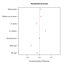
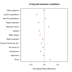
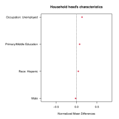
Triangular Kernel - $p=1$: $\mathcal{U}_{s_{0}}=\{i:39.0\leq S_{i}\leq 174.5\}$
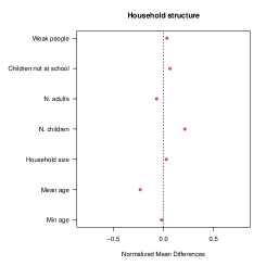
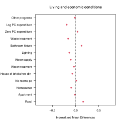
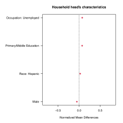
Uniform Kernel - $p=2$: $\mathcal{U}_{s_{0}}=\{i:0.0\leq S_{i}\leq 166.0\}$
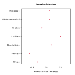
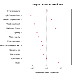
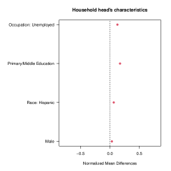
Triangular Kernel - $p=2$: $\mathcal{U}_{s_{0}}=\{i:0.0\leq S_{i}\leq 165.6\}$

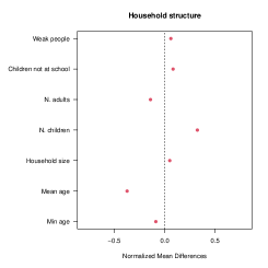
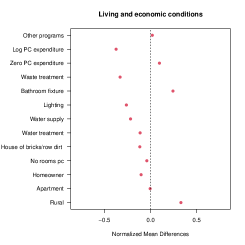
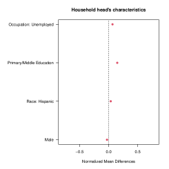
Appendix F Bayesian Causal Inference Conditional on a MSE-optimal Subpopulation: Computational Details

F.1. Likelihood Functions

We can write the observed likelihood function in terms of the observed data as follows:

$$\mathscr{L}\left(\bm{\theta}\mid\mathbf{X},\mathbf{S},\mathbf{Z},\mathbf{Y}^{obs};\mathcal{U}_{s_{0}}\right)=\mathscr{L}\left(\bm{\gamma}_{0},\bm{\gamma}_{1}\mid\mathbf{X},\mathbf{S},\mathbf{Z},\mathbf{Y}^{obs};\mathcal{U}_{s_{0}}\right)\propto$$

$$\prod\limits_{i\in\mathcal{U}_{s_{0}}:Z_{i}=0}p(Y^{obs}_{i}\mid\mathbf{X}_{i},i\in\mathcal{U}_{s_{0}};\bm{\gamma}_{0})\times\prod\limits_{i\in\mathcal{U}_{s_{0}}:Z_{i}=1}p(Y^{obs}_{i}\mid\mathbf{X}_{i},i\in\mathcal{U}_{s_{0}};\bm{\gamma}_{1})$$

In the Bolsa Família study, we have $\bm{\gamma}_{0}=(\gamma_{0,0},\bm{\gamma}_{X,0})$; $\bm{\gamma}_{1}=(\gamma_{0,1},\bm{\gamma}_{X,1})$; and we impose $\bm{\gamma}_{X,0}=\bm{\gamma}_{X,1}\equiv\bm{\gamma}_{X}$. Therefore, the observed-data likelihood is

$$\mathscr{L}\left(\bm{\theta}\mid\mathbf{X},\mathbf{S},\mathbf{Z},\mathbf{Y}^{obs};\mathcal{U}_{s_{0}}\right)=\mathscr{L}\left(\gamma_{0}^{+},\gamma_{1}^{+},\bm{\gamma}_{X},\mid\mathbf{X},\mathbf{S},\mathbf{Z},\mathbf{Y}^{obs};\mathcal{U}_{s_{0}}\right)\propto$$

$$\prod\limits_{i\in\mathcal{U}_{s_{0}}:Z_{i}=0}\Phi\left(\gamma_{0,0}+\mathbf{X}_{i}^{\prime}\bm{\gamma}_{X}\right)^{Y^{obs}_{i}}\left[1-\Phi\left(\gamma_{0,0}+\mathbf{X}_{i}^{\prime}\bm{\gamma}_{X}\right)\right]^{1-Y^{obs}_{i}}\times$$

$$\prod\limits_{i\in\mathcal{U}_{s_{0}}:Z_{i}=1}\Phi\left(\gamma_{0,1}+\mathbf{X}_{i}^{\prime}\bm{\gamma}_{X}\right)^{Y^{obs}_{i}}\left[1-\Phi\left(\gamma_{0,1}+\mathbf{X}_{i}^{\prime}\bm{\gamma}_{X}\right)\right]^{1-Y^{obs}_{i}}$$

F.2. Prior Distributions

In the Bolsa Família study, we assume that parameters are a priori independent and use proper Normal prior distributions. Specifically, the prior distributions for the parameters of the outcome models are: $\gamma_{0,z}\sim N(0,\sigma^{2}_{\gamma_{0,z}})$, $z=0,1$, and $\bm{\gamma}_{X}\sim N_{p}(\bm{0},\sigma^{2}_{\bm{\gamma}_{X}}\mathbf{I}_{p})$, where $\sigma^{2}_{\bm{\gamma}^{-}}$, $\sigma^{2}_{\bm{\gamma}^{+}}$ $\sigma^{2}_{\gamma_{0,z}}$, $z=0,1$, and $\sigma^{2}_{\bm{\gamma}_{X}}$ are hyperparameters set at $1$.

F.3. MCMC Algorithm for a selected subpopulation, $\mathcal{U}_{s_{0}}$, for the Bolsa Família study

1. Sample the coefficients $\gamma_{0,0}$ and $\gamma_{0,1}$

   1. Sample the latent variable $\mathbf{Y}^{\ast}$

      1. For $i\in\mathcal{U}_{s_{0}}$ with $Z_{i}=0$, sample the latent variable $Y_{i}^{\ast}$ from $N(\gamma_{0,0}+\mathbf{X}_{i}^{\prime}\bm{\gamma}_{X},1)$ truncated to $[0,+\infty)$ if $Y_{i}=1$ and to $(-\infty,0]$ if $Y_{i}=0$;

      2. For $i\in\mathcal{U}_{s_{0}}$ with $Z_{i}=1$, sample the latent variable $Y_{i}^{\ast}$ from $N(\gamma_{0,1}+\mathbf{X}_{i}^{\prime}\bm{\gamma}_{X},1)$ truncated to $[0,+\infty)$ if $Y_{i}=1$ and to $(-\infty,0]$ if $Y_{i}=0$;

   2. Sample the coefficient $\gamma_{0,0}$ from $N\left(\mu(\gamma_{0,0}),\sigma^{2}(\gamma_{0,0})\right)$ where

      $$\sigma^{2}(\gamma_{0,0})=\left[\dfrac{1}{\sigma^{2}_{\gamma_{0,0}}}+\sum_{i\in\mathcal{U}_{s_{0}}}(1-Z_{i})\right]^{-1}$$

      and

      $$\mu(\gamma_{0,0})=\sigma^{2}(\gamma_{0,0})\left[\dfrac{0}{\sigma^{2}_{\gamma_{0,0}}}+\sum_{i\in\mathcal{U}_{s_{0}}}(Y_{i}^{\ast}-\mathbf{X}_{i}^{\prime}\bm{\gamma}_{X})(1-Z_{i})\right]=\sigma^{2}(\gamma_{0,0})\sum_{i\in\mathcal{U}_{s_{0}}}(Y_{i}^{\ast}-\mathbf{X}_{i}^{\prime}\bm{\gamma}_{X})(1-Z_{i})$$

   3. Sample the coefficient $\gamma_{0,1}$ from $N\left(\mu(\gamma_{0,1}),\sigma^{2}(\gamma_{0,1})\right)$ where

      $$\sigma^{2}(\gamma_{0,1})=\left[\dfrac{1}{\sigma^{2}_{\gamma_{0,1}}}+\sum_{i\in\mathcal{U}_{s_{0}}}Z_{i}\right]^{-1}$$

      and

      $$\mu(\gamma_{0,1})=\sigma^{2}(\gamma_{0,1})\left[\dfrac{0}{\sigma^{2}_{\gamma_{0,1}}}+\sum_{i\in\mathcal{U}_{s_{0}}}(Y_{i}^{\ast}-\mathbf{X}_{i}^{\prime}\bm{\gamma}_{X})Z_{i}\right]=\sigma^{2}(\gamma_{0,1})\sum_{i\in\mathcal{U}_{s_{0}}}(Y_{i}^{\ast}-\mathbf{X}_{i}^{\prime}\bm{\gamma}_{X})Z_{i}$$

2. Sample the coefficients $\bm{\gamma}_{X}$

   1. Sample the latent variable $\mathbf{Y}^{\ast}$

      1. For $i\in\mathcal{U}_{s_{0}}$ with $Z_{i}=0$, sample the latent variable $Y_{i}^{\ast}$ from $N(\gamma_{0,0}+\mathbf{X}_{i}^{\prime}\bm{\gamma}_{X},1)$ truncated to $[0,+\infty)$ if $Y_{i}=1$ and to $(-\infty,0]$ if $Y_{i}=0$;

      2. For $i\in\mathcal{U}_{s_{0}}$ with $Z_{i}=1$, sample the latent variable $Y_{i}^{\ast}$ from $N(\gamma_{0,1}+\mathbf{X}_{i}^{\prime}\bm{\gamma}_{X},1)$ truncated to $[0,+\infty)$ if $Y_{i}=1$ and to $(-\infty,0]$ if $Y_{i}=0$;

   2. Let $\widetilde{Y}^{\ast}$ be a $N_{\mathcal{U}_{s_{0}}}-$dimetional vector with $N_{\mathcal{U}_{s_{0}}}=\sum_{i=1}^{N}\mathbb{I}\{i\in\mathcal{U}_{s_{0}}\}$ with $i$th element equal to

      $$\widetilde{Y}_{i}^{\ast}=\begin{cases}Y_{i}^{\ast}-\gamma_{0,0}&\hbox{if }i\in\mathcal{U}_{s_{0}},Z_{i}=0\\ Y_{i}^{\ast}-\gamma_{0,1}&\hbox{if }i\in\mathcal{U}_{s_{0}},Z_{i}=1\end{cases}$$

      and let $\mathbf{X}_{\mathcal{U}_{s_{0}}}$ the $N_{\mathcal{U}_{s_{0}}}\times p$ sub-matrix of $\mathbf{X}$ stacking information on the covariates for units in $\mathcal{U}_{s_{0}}$

   3. Sample the coefficients $\bm{\gamma}_{X}$ from $N_{p}\left(\bm{\mu}(\bm{\gamma}_{X}),\Sigma(\bm{\gamma}_{X})\right)$ where

      $$\Sigma(\bm{\gamma}_{X})=\left[\dfrac{1}{\sigma^{2}_{\bm{\gamma}_{X}}}\mathbf{I}_{p}+\mathbf{X}_{\mathcal{U}_{s_{0}}}^{\prime}\mathbf{X}_{\mathcal{U}_{s_{0}}}\right]^{-1}$$

      and

      $$\bm{\mu}(\bm{\gamma}_{X})=\Sigma(\bm{\gamma}_{X})\left[\dfrac{1}{\sigma^{2}_{\bm{\gamma}_{X}}}\mathbf{I}_{p}\bm{0}+\mathbf{X}_{\mathcal{U}_{s_{0}}}^{\prime}\widetilde{Y}^{\ast}\right]=\Sigma(\bm{\gamma}_{X})\mathbf{X}_{\mathcal{U}_{s_{0}}}^{\prime}\widetilde{Y}^{\ast}$$

Appendix G Results based on the Continuity Assumption

Local polynomial Regression Discontinuity (RD) point estimators: Calonico et al., (2018) and Calonico et al., (2019). Under the assumption that the conditional regression or distribution functions of the potential outcomes given the forcing variable, $Y_{i}(0)\mid S_{i}=s$ and $Y_{i}(1)\mid S_{i}=s$ are continuous in $s$, causal effects at the threshold can be estimated using Local polynomial Regression Discontinuity point estimators (e.g. Imbens and Lemieux, 2008; Lee and Lemieux, 2010; Calonico et al., 2014, 2018, 2014, 2019).

We use uniform and triangular kernel functions to construct the local-polynomial estimator with order of the local-polynomial equal to 1 and 2 and two sided Mean Square Error-optimal bandwidth selectors (below and above the cutoff) for the RD treatment effect estimator. Table 21 shows the results.

Table 21. Bolsa Família study: Local polynomial RD point estimators of the average treatment effect at the threshold, $ATE_{s_{0}}$, and the causal relative risk at the threshold, $RR_{s_{0}}$.

$$\begin{array}[]{cc ccc c}\hline\cr P(Y_{i}(0)=1\mid S_{i}=s_{0})&P(Y_{i}(1)=1\mid S_{i}=s_{0})&RR_{s_{0}}&ATE_{s_{0}}&\lx@intercol\hfil\hbox{95\% CI for }ATE_{s_{0}}\hfil\lx@intercol\\ \hline\cr\vspace{-0.2cm}\hfil\\ \lx@intercol\hbox{Uniform Kernel $(p=1)$: $h_{r}=43.9$ and $h_{l}=76.5$}\hfil\lx@intercol\\ \vspace{-0.4cm}\hfil\\ 0.00357&0.00280&0.78402&-0.00077&-0.00366&0.00211\\ \vspace{-0.2cm}\hfil\\ \lx@intercol\hbox{Triangular Kernel $(p=1)$: $h_{r}=54.5$ and $h_{l}=81.0$}\hfil\lx@intercol\\ \vspace{-0.4cm}\hfil\\ 0.00358&0.00311&0.86901&-0.00047&-0.00344&0.00250\\ \vspace{-0.2cm}\hfil\\ \lx@intercol\hbox{Uniform Kernel $(p=2)$: $h_{r}=46.0$ and $h_{l}=120.0$}\hfil\lx@intercol\\ \vspace{-0.4cm}\hfil\\ 0.00429&0.00283&0.65865&-0.00147&-0.00610&0.00317\\ \vspace{-0.2cm}\hfil\\ \lx@intercol\hbox{Triangular Kernel $(p=2)$: $h_{r}=45.5.9$ and $h_{l}=120.0$}\hfil\lx@intercol\\ \vspace{-0.4cm}\hfil\\ 0.00415&0.00328&0.78989&-0.00087&-0.00749&0.00575\\ \hline\cr\lx@intercol\hbox{\footnotesize{$p=$ Order of the local polynomial; $h_{l}=$ Left bandwidth ($Z_{i}=1$); $h_{r}=$ Right bandwidth ($Z_{i}=1$)}}\hfil\lx@intercol\end{array}$$

References

- Ali et al., (2019) Ali, M. S., Ichihara, M. Y., Lopes, L. C., Barbosa, G. C., Pita, R., Carreiro, R. P., Dos Santos, D. B., Ramos, D., Bispo, N., Raynal, F., et al. (2019). Administrative data linkage in brazil: potentials for health technology assessment. Frontiers in pharmacology, 10:984.
- Athey and Imbens, (2017) Athey, S. and Imbens, G. (2017). The state of applied econometrics: Causality and policy evaluation. Journal of Economic Perspectives, 31(2):3–32.
- Barbosa and Corseuil, (2014) Barbosa, A. L. N. d. H. and Corseuil, C. H. L. (2014). Conditional cash transfer and informality in brazil. IZA Journal of Labor & Development, 3(1):1–18.
- Barbosa et al., (2020) Barbosa, G. C. G., Ali, M. S., Araujo, B., Reis, S., Sena, S., Ichihara, M. Y. T., Pescarini, J., Fiaccone, R. L., Amorim, L. D., Pita, R., Barreto, M. E., Smeeth, L., and Barreto, M. L. (2020). Cidacs-rl: a novel indexing search and scoring-based record linkage system for huge datasets with high accuracy and scalability. BMC Med Inform Decis Mak, 20(1):289.
- Barreto et al., (2019) Barreto, M., Ichihara, M., de Almeida, B., Barreto, M. P., da Rocha Cabral, L., Fiaccone, R., Carreiro, R., Teles, C. C. G. D., Pitta, R. G., Penna, G., Barral-Netto, M., Ali, M. M., Barbosa, G. C. G., Denaxas, S. C., Rodrigues, L., and Smeeth, L. (2019). The centre for data and knowledge integration for health (cidacs): Linking health and social data in brazil. International Journal of Population Data Science, 4.
- Battistin and Rettore, (2008) Battistin, E. and Rettore, E. (2008). Ineligibles and eligible non-participants as a double comparison group in regression-discontinuity designs. Journal of Econometrics, 142:715–730.
- Bonvini and Kennedy, (2022) Bonvini, M. and Kennedy, E. H. (2022). Sensitivity analysis via the proportion of unmeasured confounding. Journal of the American Statistical Association, 117(539):1540–1550.
- Borusyak et al., (2023) Borusyak, K., Hull, P., and Jaravel, X. (2023). Design-based identification with formula instruments: A review. NBER Working Paper Series, (31393).
- Branson and Mealli, (2019) Branson, Z. and Mealli, F. (2019). The local randomization framework for regression discontinuity designs: A review and some extensions. arXiv preprint arXiv:1810.02761.
- Calonico et al., (2018) Calonico, S., Cattaneo, M. D., and Farrell, M. H. (2018). On the effect of bias estimation on coverage accuracy in nonparametric inference. Journal of the American Statistical Association, 113(522):767–779.
- Calonico et al., (2019) Calonico, S., Cattaneo, M. D., Farrell, M. H., and Titiunik, R. (2019). Regression Discontinuity Designs Using Covariates. The Review of Economics and Statistics, 101(3):442–451.
- Calonico et al., (2014) Calonico, S., Cattaneo, M. D., and Titiunik, R. (2014). Robust nonparametric confidence intervals for regression-discontinuity designs. Econometrica, 82(6):2295–2326.
- Calonico et al., (2015) Calonico, S., Cattaneo, M. D., and Titiunik, R. (2015). rdrobust: An r package for robust nonparametric inference in regression-discontinuity designs. R Journal, 7(1):38–51.
- Cattaneo et al., (2015) Cattaneo, M., Frandsen, B. R., and Titiunik, R. (2015). Randomization inference in the regression discontinuity design: An application to party advantages in the u.s. senate. Journal of Causal Inference, 3(1):1–24.
- Cattaneo and Escanciano, (2017) Cattaneo, M. D. and Escanciano, J. C. (2017). Regression Discontinuity Designs: Theory and Applications, volume 38. Emerald Group Publishing.
- (16) Cattaneo, M. D., Idrobo, N., and Titiunik, R. (2020a). A Practical Introduction to Regression Discontinuity Designs: Extensions. Cambridge University Press.
- (17) Cattaneo, M. D., Idrobo, N., and Titiunik, R. (2020b). A Practical Introduction to Regression Discontinuity Designs: Foundations. Cambridge University Press.
- (18) Cattaneo, M. D., Titiunik, R., and Vazquez-Bare, G. (2020c). The regression discontinuity design. In Publications, S., editor, Handbook of Research Methods in Political Science and International Relations, volume Chapter 44, pages 835–857.
- Diebolt and Robert, (1994) Diebolt, J. and Robert, C. P. (1994). Estimation of finite mixture distributions through bayesian sampling. Journal of the Royal Statistical Society: Series B (Methodological), 56(2):363–375.
- Dourado et al., (2017) Dourado, A., Carvalho, R. N., and van Erven, G. C. G. (2017). Brazil’s bolsa familia and young adult workers: A parallel rdd approach to large datasets. In 2017 International Joint Conference on Neural Networks (IJCNN), pages 17–24.
- Eckles et al., (2020) Eckles, D., Ignatiadis, N., Wager, S., and Wu, H. (2020). Noise-induced randomization in regression discontinuity designs.
- Firpo et al., (2014) Firpo, S., Pieri, R., Pedroso Jr, E., and Souza, A. P. (2014). Evidence of eligibility manipulation for conditional cash transfer programs. Economica, 15(3):243–260.
- Hahn et al., (2001) Hahn, J., Todd, P., and der Klaauw, W. V. (2001). Identification and estimation of treatment effects with a regression-discontinuity design. Econometrica, 69(1):201–209.
- Hirano et al., (2000) Hirano, K., Imbens, G. W., Rubin, D. B., and Zhou, X.-H. (2000). Assessing the effect of an influenza vaccine in an encouragement design. Biostatistics, 1(1):69–88.
- Imbens and Rubin, (1997) Imbens, G. and Rubin, D. (1997). Bayesian inference for causal effects in randomized experiments with noncompliance. The Annals of Statistics, 25(1):305–327.
- Imbens and Kalyanaraman, (2012) Imbens, G. W. and Kalyanaraman, K. (2012). Optimal bandwidth choice for the regression discontinuity estimator. Review of Economic Studies, 79(3):933–959.
- Imbens and Lemieux, (2008) Imbens, G. W. and Lemieux, T. (2008). Regression discontinuity designs: A guide to practice. Journal of Econometrics, 142:615–635.
- Imbens and Rubin, (2015) Imbens, W. and Rubin, D. (2015). Causal Inference for Statistics, Social, and Biomedical Sciences. An Introduction. Cambridge University Press, New York, NY, USA.
- Keele et al., (2015) Keele, L., Titiunik, R., and Zubizarreta, J. R. (2015). Enhancing a geographic regression discontinuity design through matching to estimate the effect of ballot initiatives on voter turnout. Journal of the Royal Statistical. Society, Series A, 178(1):223–239.
- Lee and Lemieux, (2010) Lee, D. S. and Lemieux, T. (2010). Regression discontinuity designs in economics. Journal of Economic Literature, 485:281–355.
- Li et al., (2023) Li, F., Ding, P., and Mealli, F. (2023). Bayesian causal inference: a critical review. Philosophical Transactions of the Royal Society A, 381(2247):20220153.
- Li et al., (2015) Li, F., Mattei, A., and Mealli, F. (2015). Bayesian inference for regression discontinuity designs with application to the evaluation of italian university grants. The Annals of Applied Statistics, 9(4):1906–1931.
- Licari and Mattei, (2020) Licari, F. and Mattei, A. (2020). Assessing causal effects of extra compulsory learning on college students’ academic performances. Journal of the Royal Statistical Society: Series A (Statistics in Society), 183(4):1595–1614.
- Linero and Antonelli, (2023) Linero, A. R. and Antonelli, J. L. (2023). The how and why of bayesian nonparametric causal inference. Wiley Interdisciplinary Reviews: Computational Statistics, 15(1):e1583.
- Mattei and Mealli, (2007) Mattei, A. and Mealli, F. (2007). Application of the principal stratification approach to the faenza randomized experiment on breast self-examination. Biometrics, 63(2):437–446.
- Mattei and Mealli, (2016) Mattei, A. and Mealli, F. (2016). Regression discontinuity designs as local randomized experiments. comment on reprint “regression-discontinuity analysis: An alternative to the ex-post facto experiment” by donald thistlewaite and donald campbell. Observational Studies, 2:156–173.
- McCrary, (2008) McCrary, J. (2008). Manipulation of the running variable in the regression discontinuity design: A density test. Journal of econometrics, 142(2):698–714.
- McLachlan and Basford, (1988) McLachlan, G. and Basford, K. (1988). Mixture Models: Inference and Application to Clustering. Marcel Dekker, New York, NY, USA.
- Mitra et al., (2017) Mitra, N., Ogburn, E., Roy, J., Shortreed, S., Small, D., and Stuart, E. (2017). Reprint “regression-discontinuity analysis: An alternative to the ex-post facto experiment” by donald thistlewaite and donald campbell and comments. Observational Studies, 3(2):119–209.
- Nilsson and Sjöberg, (2013) Nilsson, H. and Sjöberg, K. (2013). An evaluation of the impacts of bolsa família on schooling. Department of Economics. University of Lund.
- Pescarini et al., (2020) Pescarini, J. M., Williamson, E., Ichihara, M. Y. T., Fiaccone, R. L., Forastiere, L., Ramond, A., Nery, J. S., Penna, M. L. F., Strina, A., Reis, S., Smeeth, L., Rodrigues, L. C., Brickley, E. B., de Oliveira Penna, G., and Barreto, M. L. (2020). Conditional cash transfer program and leprosy incidence: Analysis of 12.9 million families from the 100 million brazilian cohort. American Journal of Epidemiology, 189:1547 – 1558.
- Pita et al., (2018) Pita, R., Pinto, C., Sena, S., Fiaccone, R., Amorim, L., Reis, S., Barreto, M. L., Denaxas, S., and Barreto, M. E. (2018). On the accuracy and scalability of probabilistic data linkage over the brazilian 114 million cohort. IEEE journal of biomedical and health informatics, 22(2):346–353.
- Ricciardi et al., (2020) Ricciardi, F., Liverani, S., and Baio, G. (2020). Dirichlet process mixture models for regression discontinuity designs. arXiv preprint arXiv:2003.11862.
- Richardson and Green, (1997) Richardson, S. and Green, P. J. (1997). On bayesian analysis of mixtures with an unknown number of components (with discussion). Journal of the Royal Statistical Society: Series B (Statistical Methodology), 59(4):731–792.
- Rubin, (1987) Rubin, D. (1987). Multiple Imputation for Nonresponse in Surveys. Wiley, New York, NY, USA.
- Rubin, (1974) Rubin, D. B. (1974). Estimating causal effects of treatments in randomized and nonrandomized studies. Journal of Educational Psychology, 66:688–701.
- Rubin, (1978) Rubin, D. B. (1978). Bayesian inference for causal effects: The role of randomization. The Annals of Statistics, 6:34–58.
- Rubin, (1980) Rubin, D. B. (1980). Discussion of “randomization analysis of experimental data in the fisher randomization test” by basu. Journal of the American Statistical Association, 75:591–593.
- Sales and Hansen, (2020) Sales, A. and Hansen, B. B. (2020). Limitless regression discontinuity. Journal of Educational and Behavioral Statistics, 45(2):143–174.
- Superti, (2020) Superti, L. H. (2020). Effects on fertility of the brazilian cash transfer program: Evidence from a regression discontinuity approach. Available at SSRN 3484588.
- Tanner and Wong, (1987) Tanner, M. A. and Wong, W. H. (1987). The calculation of posterior distributions by data augmentation. Journal of the American Statistical Association, 82(398):528–540.
- Thistlethwaite and Campbell, (1960) Thistlethwaite, D. and Campbell, D. (1960). Regression-discontinuity analysis: an alternative to the ex-post facto experiment. Journal of Educational Psychology, 51(6):309–317.
- Titterington et al., (1985) Titterington, D., Smith, A., and Markov, U. (1985). Statistical Analysis of Finite Mixture Distributions. John Wiley & Sons.